1

Chapter 2: Mass Balance - The Cornerstone of Chemical Oceanography (10/11/04) James W. Murray Univ. Washington The chemical distributions on the earth and in the ocean reflect transport and transformation processes, many of which are cyclic. The cycling of water from the ocean to the atmosphere to land and back to the ocean via rivers is such an example. This basic cycling is often described in terms of the content of the various reservoirs (e.g., the ocean, the atmosphere, etc.) and the fluxes between them (e.g., evaporation, rivers, etc.). A fundamental question is how the rates of transfer between the reservoirs depends on the content of the reservoirs and on other external factors. The details of the distributions within the reservoirs is neglected. Most oceanographers construct simple models to test their understanding of the essential elements of the system and to predict the response of a system to perturbations and forcings. The principal of Ockham's Razor has served oceanographers well. This principle states that: When seeking to explain phenomena, start with the simplest theory (see Safire, 1999, for the etymology). A few words about the scientific method. Some fields of science are advancing more rapidly than others. It is the contention of Platt (1964) that those rapidly advancing fields are those where the method of doing research called "strong inference" is systematically used and taught. Strong inference consists of formally and explicitly applying the following steps to every problem. 1) Devising alternative hypotheses 2) Devising a crucial experiment (or experiments) with alternative possible outcomes

each of which will, as nearly as possible, exclude one of more of the hypotheses 3) Carrying out the experiment so as to get a clean result. 1') Recycling the procedure to refine the hypotheses that remain. Scientific hypotheses are most securely "validated" when (i) they make successful predictions; (ii) there are conceivable observations that could, in principle, refute them, but have not; and (iii) there is a comparably sensible competitor theory that is faring worse. Developing alternative simple models is part of this process. The purpose of this chapter is to introduce the tools necessary to develop the two main types of models used in chemical oceanography. These are:. -Box (or reservoir) Models and -Continuous Transport-reaction Models First some basic definitions related to models in general and box or reservoir models.

2

- Model - A simplified or idealized description of a particular system or process that is put forward as a basis for calculations, predictions or further investigation. A model should contain only those elements of reality that are needed to solve the problem. The least necessary model is the best possible model for the purpose. A model is an imitation of reality which stresses those aspects that are assumed to be important and omits all properties considered to be nonessential. A model is like a caricature of a real system.

- Parameter - A quantity which is constant (as distinct from ordinary variables) in a particular case considered, but which varies in different cases. An independent variable in terms of which each co-ordinate of a point is expressed.

- Variable - A quantity or force which, throughout a mathematical calculation or investigation, is assumed to vary or be capable of varying in value.

- Closure - Closure in a modeling sense usually means having the number of unknowns equal the number of equations. Often, closure is achieved by making simplifying assumptions.

- Reservoir (M)(also box or compartment) - The amount of material contained by a defined physical regime, such as the atmosphere, the surface ocean or the lithosphere. The size of the reservoirs are determined by the scale of the analysis as well as the homogeneity of the spatial distribution. The units are usually in mass of moles.

- Flux (F) - The amount of material transferred from one reservoir to another per unit time.

- Source (Q) - A flux of material into a reservoir. - Sink (S) - A flux of material out of a reservoir - Budget - A balance equation of all sources and sinks for a given reservoir. - Turnover Time (τ) - The ratio of the content (M) of a reservoir divided by the sum

of its sources (ΣQ) or sinks (ΣS). Thus τ = M/ΣQ or τ = M/ΣS. - Cycle - A system consisting of two or more connected reservoirs where a large

fraction of the material is transferred through the system in a cyclic fashion. Budgets and cycles can be considered over a wide range of spatial scales from local to global.

- Steady State - When the sources and sinks are in balance and do not change with time.

- Closed System - When all the material cycles within the system - Open System - When material exchanges with outside the system. A. Mass Balance - Simple Box Models Many processes may act to control the distributions of chemicals in the ocean. The method of putting these processes together in a model utilizes the principle of mass balance applied to the system as a whole or some parts of it (control volumes). Control volumes or boxes are connected by internal transport processes such as advection and diffusion. The system as a whole is linked to the environment by external inputs and outputs. Box models are especially useful for understanding geochemical cycles and their dynamic response to change.

3

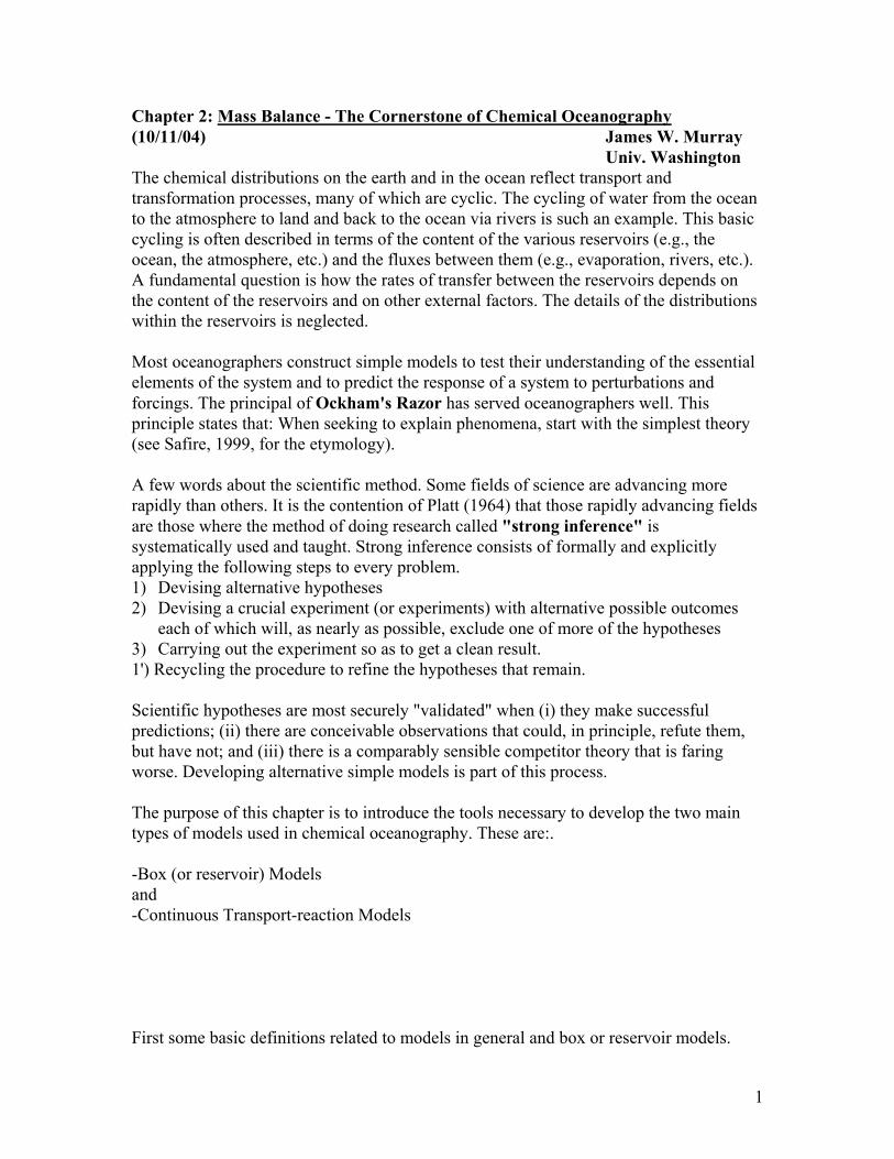
The framework of box models for geochemical cycles is conceptually similar to chemical kinetic reactions and similar equations are used to describe the stability of chemical and biochemical systems (Prigogine, 1967). The Lotka-Voltera preditor-prey model of population dynamics is a classic example of the such equations. Describing a model first requires choosing a system, that is, the division between what is "in" and what is "out". The second step involves choosing the complexity of the description of the "internal" system. The goal in modeling is to analyze all the relevant processes simultaneously. The concept of mass balance serves as a way to link everything together. To use the idea of a mass balance, the system is first divided into one or several "control volumes" which are connected with each other and the rest of the world by mass fluxes. A mass balance equation is written for each control volume and each chemical The Change in = Sum of + Sum of Internal - Sum of - Sum of all Mass with Time all Inputs Sources Outputs Internal Sinks Such box models are used to determine the rates of transfer between reservoirs and transformations within a reservoir. Advantages are: 1. They are easy to conceptualize and visualize where material is coming from and going to. 2. They provide an overview of fluxes, reservoir sizes and turnover or residence times (τ) 3. They provide the basis for more detailed quantitative models 4. They help identify gaps in knowledge Disadvantages are: 1. The analysis is superficial 2. Little or no insight is gained into what goes on inside the reservoirs or into the nature of the fluxes between them. 3. It usually assumes homogeneous average distributions within reservoirs 4. They can easily give a false impression of certainty, even if all the individual fluxes have solid estimates. Remember, a model is an imitation of reality. Introduce the concept of Steady State and Residence Time We can draw a one box model of the ocean with the main fluxes indicated. These include river and glacial input, atmospheric exchange, hydrothermal exchange and sediment exchange. Rivers and glaciers are shown here as ocean sources. The other fluxes can go both ways. Radioactive decay is a source or sink for radioactive elements in the ocean. The total dissolved mass in the box is called M and is assumed to be homogeneously distributed in the box.

4

Simple 1-Box Ocean Atmosphere +dM/dt Rivers (+dM/dt) Glaciers (+dM/dt) RadR Sediments Hydrothermal At steady state the dissolved concentration (Mi) does not change with time:

(dM/dt)ocn = ΣdMi / dt 1 At steady state the sum of the sources Σ(dM/dt)sources must equal the sum of the sinks Σ(dM/dt)sinks. Is the 1-Box ocean at steady state? This is difficult to verify. How would you do this? You could measure the composition with time. You could check to see if the sources and sinks were in balance. Both have large uncertainties. The confidence with which we can claim steady state exists is usually low when the uncertainties of the fluxes are propagated through to the final result. For most elements the main sources are from continents via the atmosphere and rivers. Removal to the sediments is a main sink for all elements. Hydrothermal processes can be both sources and sinks depending on the element. The following balance is a good approximation for most elements in the ocean: (dn/dt)ocn = Fatm + Frivers - Fseds + Fhydrothermal 2 If we assume steady state then the change with time is zero or (dM /dt)ocn = 0. We can also assume that the atmospheric flux is negligible for most elements. Then the main balance for most elements is the even simpler equation: Frivers = Fsediment + Fhydrothermal 3

Ocean Radiodecay + dM/dt

+dM/dt +dM/dt

Mt

5

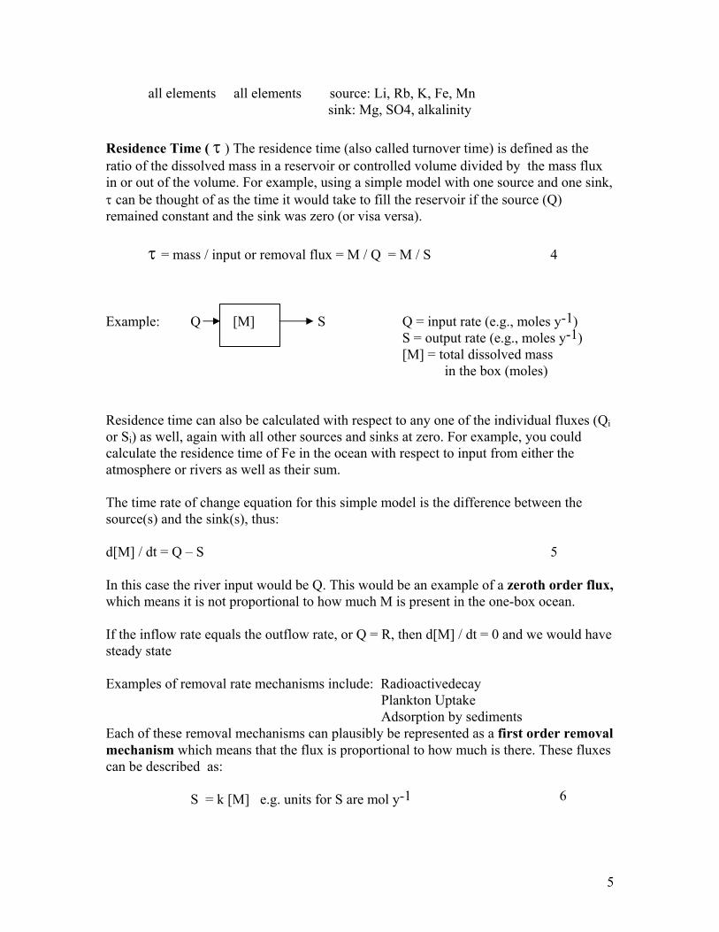
all elements all elements source: Li, Rb, K, Fe, Mn sink: Mg, SO4, alkalinity Residence Time ( τ ) The residence time (also called turnover time) is defined as the ratio of the dissolved mass in a reservoir or controlled volume divided by the mass flux in or out of the volume. For example, using a simple model with one source and one sink, τ can be thought of as the time it would take to fill the reservoir if the source (Q) remained constant and the sink was zero (or visa versa). τ = mass / input or removal flux = M / Q = M / S 4 Example: Q [M] S Q = input rate (e.g., moles y-1) S = output rate (e.g., moles y-1) [M] = total dissolved mass

in the box (moles) Residence time can also be calculated with respect to any one of the individual fluxes (Qi or Si) as well, again with all other sources and sinks at zero. For example, you could calculate the residence time of Fe in the ocean with respect to input from either the atmosphere or rivers as well as their sum. The time rate of change equation for this simple model is the difference between the source(s) and the sink(s), thus: d[M] / dt = Q – S 5 In this case the river input would be Q. This would be an example of a zeroth order flux, which means it is not proportional to how much M is present in the one-box ocean. If the inflow rate equals the outflow rate, or Q = R, then d[M] / dt = 0 and we would have steady state Examples of removal rate mechanisms include: Radioactivedecay Plankton Uptake Adsorption by sediments Each of these removal mechanisms can plausibly be represented as a first order removal mechanism which means that the flux is proportional to how much is there. These fluxes can be described as: S = k [M] e.g. units for S are mol y-1 6

6

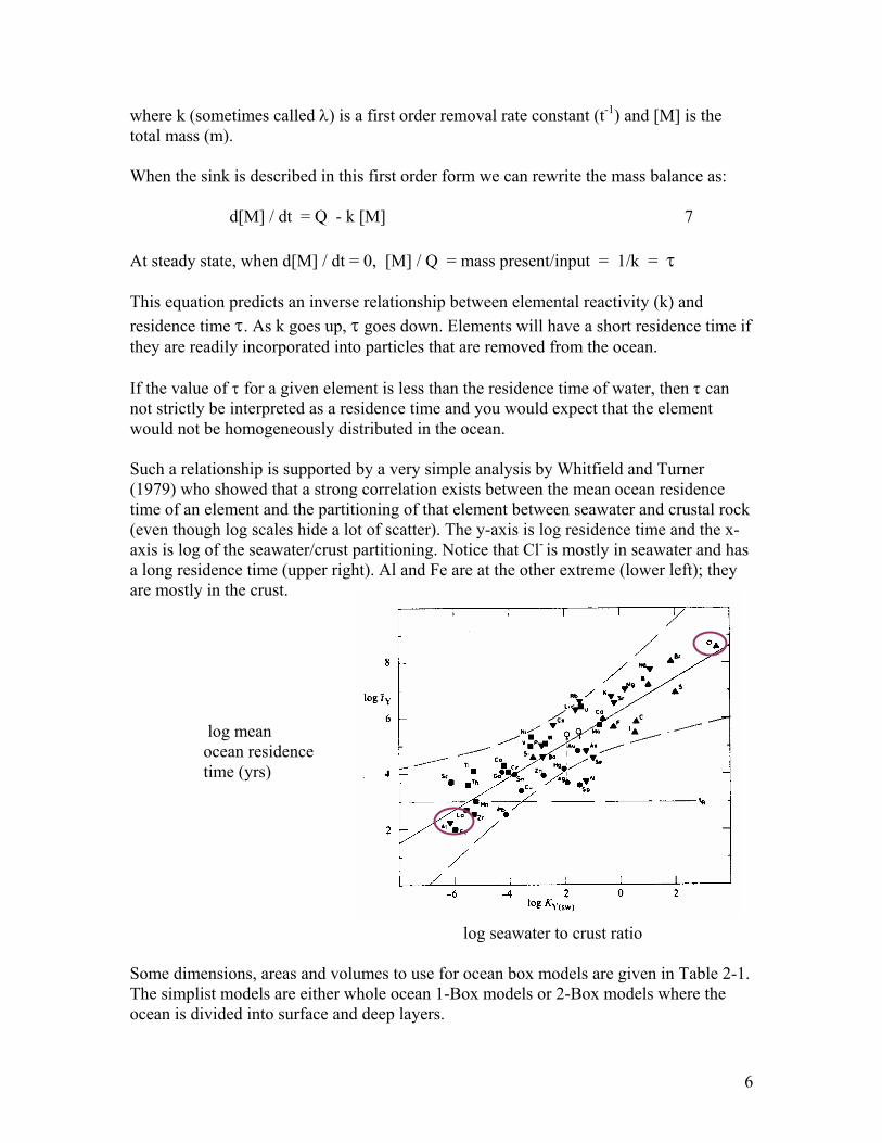
where k (sometimes called λ) is a first order removal rate constant (t-1) and [M] is the total mass (m). When the sink is described in this first order form we can rewrite the mass balance as: d[M] / dt = Q - k [M] 7 At steady state, when d[M] / dt = 0, [M] / Q = mass present/input = 1/k = τ This equation predicts an inverse relationship between elemental reactivity (k) and residence time τ. As k goes up, τ goes down. Elements will have a short residence time if they are readily incorporated into particles that are removed from the ocean. If the value of τ for a given element is less than the residence time of water, then τ can not strictly be interpreted as a residence time and you would expect that the element would not be homogeneously distributed in the ocean. Such a relationship is supported by a very simple analysis by Whitfield and Turner (1979) who showed that a strong correlation exists between the mean ocean residence time of an element and the partitioning of that element between seawater and crustal rock (even though log scales hide a lot of scatter). The y-axis is log residence time and the x-axis is log of the seawater/crust partitioning. Notice that Cl- is mostly in seawater and has a long residence time (upper right). Al and Fe are at the other extreme (lower left); they are mostly in the crust. log mean ocean residence time (yrs) log seawater to crust ratio Some dimensions, areas and volumes to use for ocean box models are given in Table 2-1. The simplist models are either whole ocean 1-Box models or 2-Box models where the ocean is divided into surface and deep layers.

7

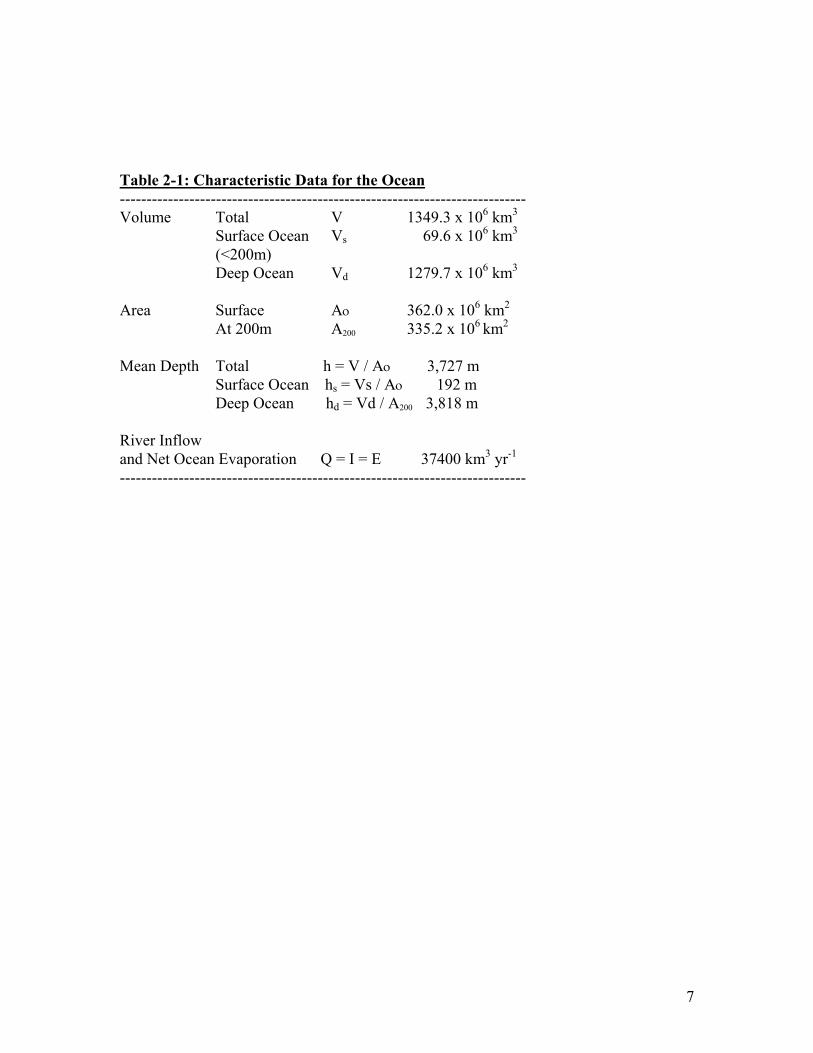
Table 2-1: Characteristic Data for the Ocean ---------------------------------------------------------------------------- Volume Total V 1349.3 x 106 km3 Surface Ocean Vs 69.6 x 106 km3

(<200m) Deep Ocean Vd 1279.7 x 106 km3 Area Surface Aο 362.0 x 106 km2 At 200m A200 335.2 x 106 km2

Mean Depth Total h = V / Aο 3,727 m Surface Ocean hs = Vs / Aο 192 m Deep Ocean hd = Vd / A200 3,818 m River Inflow and Net Ocean Evaporation Q = I = E 37400 km3 yr-1 ----------------------------------------------------------------------------

8

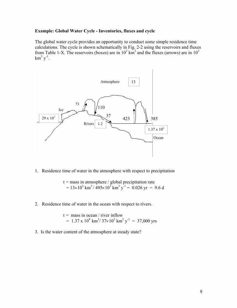
Example: Global Water Cycle - Inventories, fluxes and cycle The global water cycle provides an opportunity to conduct some simple residence time calculations. The cycle is shown schematically in Fig. 2-2 using the reservoirs and fluxes from Table 1-X. The reservoirs (boxes) are in 103 km3 and the fluxes (arrows) are in 103 km3 y-1.

1. Residence time of water in the atmosphere with respect to precipitation

τ = mass in atmosphere / global precipitation rate = 13×103 km3 / 495×103 km3 y-1 = 0.026 yr = 9.6 d 2. Residence time of water in the ocean with respect to rivers.

τ = mass in ocean / river inflow = 1.37 x 109 km3/ 37×103 km3 y-1 = 37,000 yrs 3. Is the water content of the atmosphere at steady state?

Atmosphere

Ocean

Ice

1.37 x 106

Atmosphere 13

Ice

29 x 103

73

423 385 37

Rivers 1.2

110

9

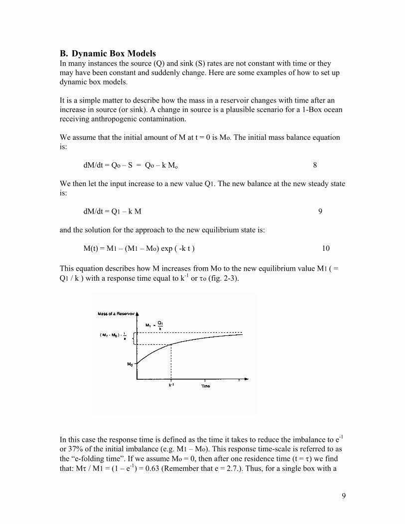
B. Dynamic Box Models In many instances the source (Q) and sink (S) rates are not constant with time or they may have been constant and suddenly change. Here are some examples of how to set up dynamic box models. It is a simple matter to describe how the mass in a reservoir changes with time after an increase in source (or sink). A change in source is a plausible scenario for a 1-Box ocean receiving anthropogenic contamination. We assume that the initial amount of M at t = 0 is Mo. The initial mass balance equation is: dM/dt = Qo – S = Qo – k Mo 8 We then let the input increase to a new value Q1. The new balance at the new steady state is: dM/dt = Q1 – k M 9 and the solution for the approach to the new equilibrium state is: M(t) = M1 – (M1 – Mo) exp ( -k t ) 10 This equation describes how M increases from Mo to the new equilibrium value M1 ( = Q1 / k ) with a response time equal to k-1 or τo (fig. 2-3).

In this case the response time is defined as the time it takes to reduce the imbalance to e-1 or 37% of the initial imbalance (e.g. M1 – Mo). This response time-scale is referred to as the “e-folding time”. If we assume Mo = 0, then after one residence time (t = τ) we find that: Mτ / M1 = (1 – e-1) = 0.63 (Remember that e = 2.7.). Thus, for a single box with a

10

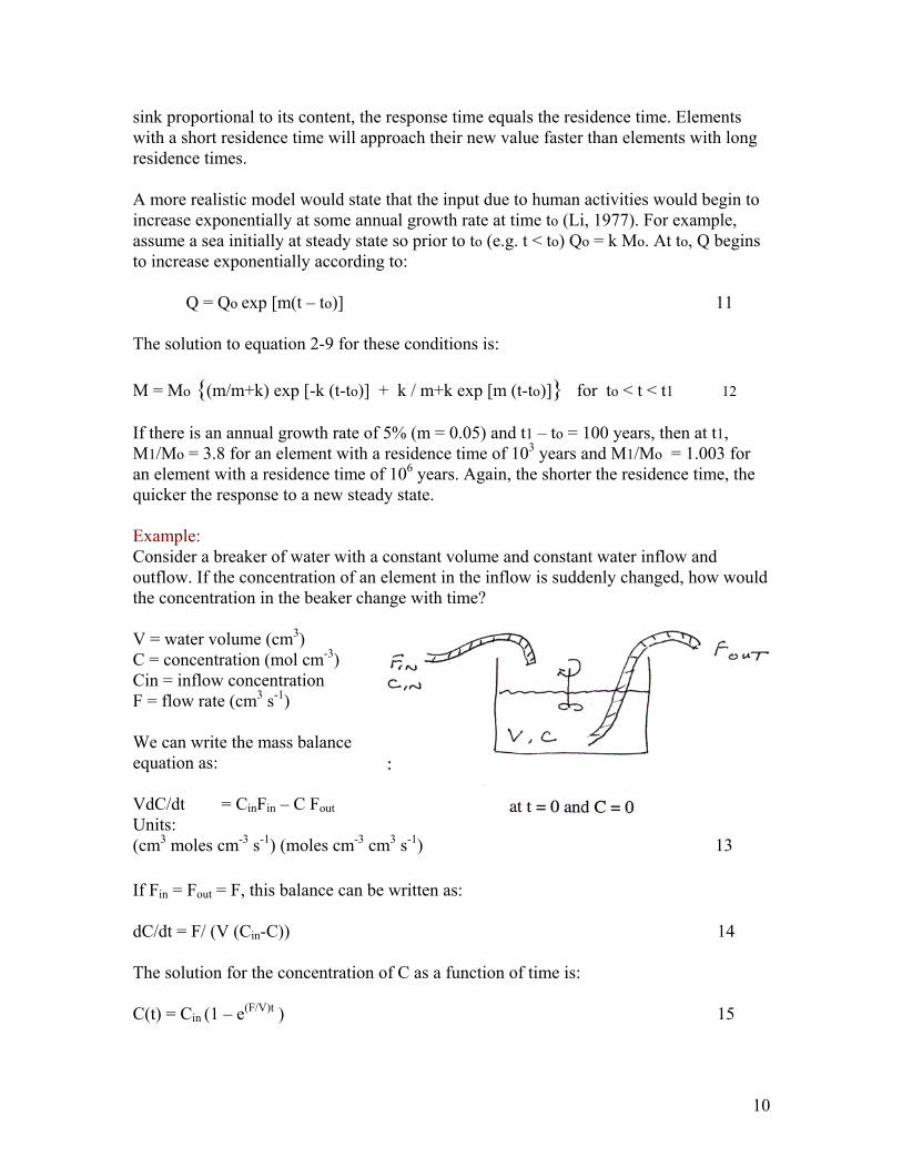
sink proportional to its content, the response time equals the residence time. Elements with a short residence time will approach their new value faster than elements with long residence times. A more realistic model would state that the input due to human activities would begin to increase exponentially at some annual growth rate at time to (Li, 1977). For example, assume a sea initially at steady state so prior to to (e.g. t < to) Qo = k Mo. At to, Q begins to increase exponentially according to: Q = Qo exp [m(t – to)] 11 The solution to equation 2-9 for these conditions is: M = Mo {(m/m+k) exp [-k (t-to)] + k / m+k exp [m (t-to)]} for to < t < t1 12 If there is an annual growth rate of 5% (m = 0.05) and t1 – to = 100 years, then at t1, M1/Mo = 3.8 for an element with a residence time of 103 years and M1/Mo = 1.003 for an element with a residence time of 106 years. Again, the shorter the residence time, the quicker the response to a new steady state. Example: Consider a breaker of water with a constant volume and constant water inflow and outflow. If the concentration of an element in the inflow is suddenly changed, how would the concentration in the beaker change with time? V = water volume (cm3) C = concentration (mol cm-3) Cin = inflow concentration F = flow rate (cm3 s-1) We can write the mass balance equation as: VdC/dt = CinFin – C Fout Units: (cm3 moles cm-3 s-1) (moles cm-3 cm3 s-1) 13 If Fin = Fout = F, this balance can be written as: dC/dt = F/ (V (Cin-C)) 14 The solution for the concentration of C as a function of time is: C(t) = Cin (1 – e(F/V)t ) 15

11

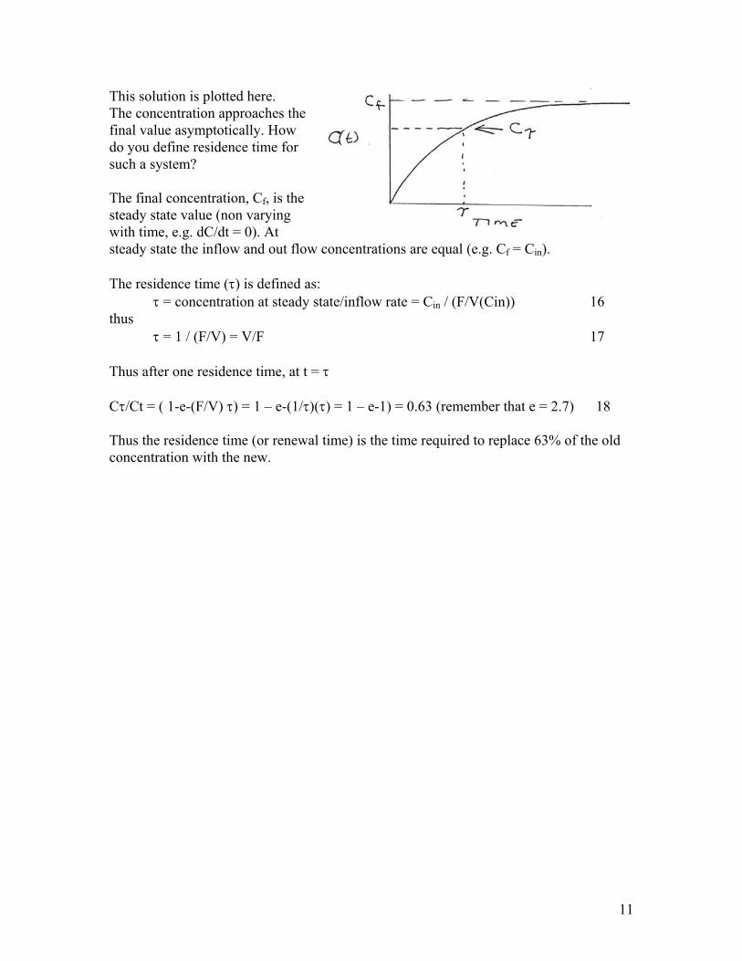
This solution is plotted here. The concentration approaches the final value asymptotically. How do you define residence time for such a system? The final concentration, Cf, is the steady state value (non varying with time, e.g. dC/dt = 0). At steady state the inflow and out flow concentrations are equal (e.g. Cf = Cin). The residence time (τ) is defined as: τ = concentration at steady state/inflow rate = Cin / (F/V(Cin)) 16 thus τ = 1 / (F/V) = V/F 17 Thus after one residence time, at t = τ Cτ/Ct = ( 1-e-(F/V) τ) = 1 – e-(1/τ)(τ) = 1 – e-1) = 0.63 (remember that e = 2.7) 18 Thus the residence time (or renewal time) is the time required to replace 63% of the old concentration with the new.

12

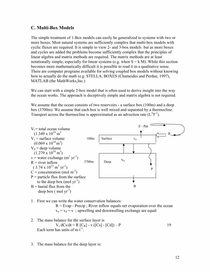
C. Multi-Box Models The simple treatment of 1-Box models can easily be generalized to systems with two or more boxes. Most natural systems are sufficiently complex that multi-box models with cyclic fluxes are required. It is simple to view 2- and 3-box models but as more boxes and cycles are added the problems become sufficiently complex that the principles of linear algebra and matrix methods are required. The matrix methods are at least notationally simple, especially for linear systems (e.g. when S = k M). While this section becomes more mathematically difficult it is possible to read it in a qualitative sense. There are computer programs available for solving coupled box models without knowing how to actually do the math (e.g. STELLA, BOXES (Chameides and Perdue, 1997), MATLAB (the MathWorks,Inc.) We can start with a simple 2-box model that is often used to derive insight into the way the ocean works. The approach is deceptively simple and matrix algebra is not required. We assume that the ocean consists of two reservoirs - a surface box (100m) and a deep box (3700m). We assume that each box is well mixed and separated by a thermocline. Transport across the thermocline is approximated as an advection rate (L3T-1). Vt = total ocean volume (1.349 x 1018 m3 Vs = surface volume (0.069 x 1018 m3) Vd = deep volume (1.279 x 1018 m3) v = water exchange (m3 yr-1) R = river inflow ( 3.74 x 1013 m3 yr-1) C = concentration (mol m-3) P = particle flux from the surface to the deep box (mol yr-1) B = burial flux from the deep box ( mol yr-1) 1. First we can write the water conservation balances:

R = Evap - Precip ; River inflow equals net evaporation over the ocean vu = vd = v ; upwelling and downwelling exchange are equal

2. The mass balance for the surface layer is Vs dCs/dt = R [CR] - v ([Cs] - [Cd]) – P 19

Each term has units of m t-1. 3. The mass balance for the deep layer is:

Surface

Deep

100m

3700m

P

B

R

vu

vd

E - Ppt

13

Vd d[Cd] / dt = v ([Cs] - [Cd]) + P – B 20 4. At steady state we have:

d[Ct] / dt = 0 and R[CR] = B 21 As an example of what can be learned we compare river inflow, R with the seawater exchange between the boxes, v. If we assume that the deep-water, with a volume Vd, has an age of 1000yrs (from 14C) Then, since τ = Vd / v we can rearrange this to estimate v as Vd / τ. or: v = (3700/3800)(1.37 x 1018 m3) / 1000yrs = 1.3 x 1015 m3 yr-1 22 River inflow is 3.7 x 1013 m3 yr-1 , thus the ratio of river inflow / deep box exchange = 3.7 x 1013 / 1.3 x 1015 = 1 / 38. This means that water circulates on average about 40 times through the ocean, between the surface and deep boxes, before it evaporates. If the ocean mixing time (deep water age) is 1000 yr, the water residence time with respect to evaporation is 40,000 yr (or 40 kyr). We set up the simple 2-Box model using matrix notation in Appendix I.

14

Transport-Reaction Models There are basically two kinds of transport

1) Direct transport due to the motion of the medium (e.g. advection) or due to external forces such as gravity (e.g. particle sinking). and 2) Random transport leading to molecular or turbulent diffusion

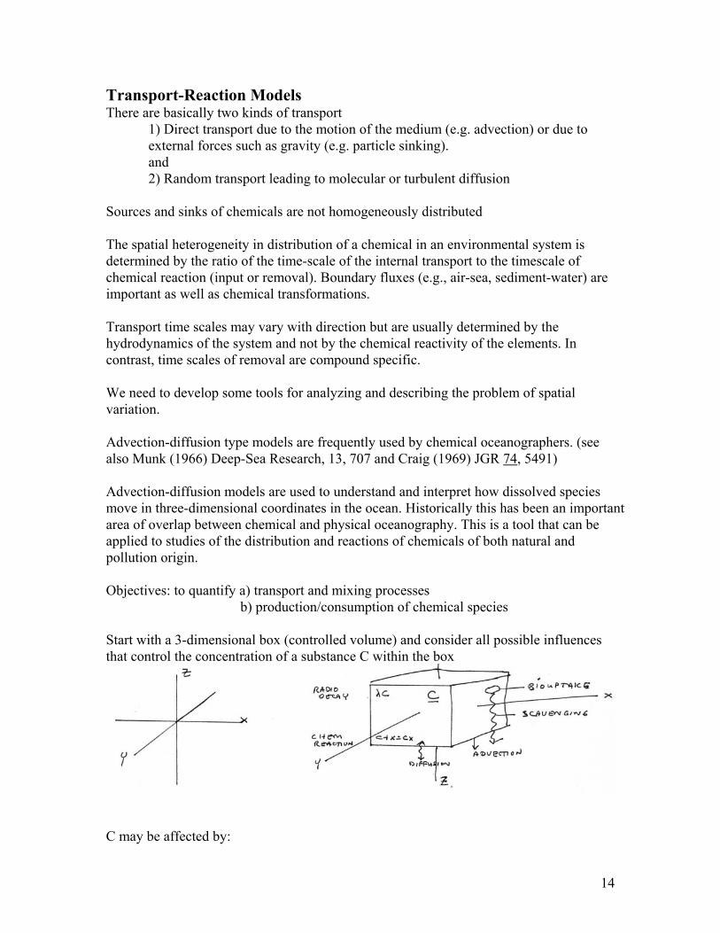
Sources and sinks of chemicals are not homogeneously distributed The spatial heterogeneity in distribution of a chemical in an environmental system is determined by the ratio of the time-scale of the internal transport to the timescale of chemical reaction (input or removal). Boundary fluxes (e.g., air-sea, sediment-water) are important as well as chemical transformations. Transport time scales may vary with direction but are usually determined by the hydrodynamics of the system and not by the chemical reactivity of the elements. In contrast, time scales of removal are compound specific. We need to develop some tools for analyzing and describing the problem of spatial variation. Advection-diffusion type models are frequently used by chemical oceanographers. (see also Munk (1966) Deep-Sea Research, 13, 707 and Craig (1969) JGR 74, 5491) Advection-diffusion models are used to understand and interpret how dissolved species move in three-dimensional coordinates in the ocean. Historically this has been an important area of overlap between chemical and physical oceanography. This is a tool that can be applied to studies of the distribution and reactions of chemicals of both natural and pollution origin. Objectives: to quantify a) transport and mixing processes b) production/consumption of chemical species Start with a 3-dimensional box (controlled volume) and consider all possible influences that control the concentration of a substance C within the box

C may be affected by:

15

1. advection (currents) 2. diffusion (random motion) 3. consumption (scavenging, chemical reaction, radioactive decay 4. production (remineralization, chem reaction, radioactive production) We combine the effect of the two main transport mechanisms (advection and diffusion) with simple in situ expressions of reaction. The transport can be expressed as the combined action of advective and diffusive transport on the temporal variation of the concentration, C: (∂c/∂t)trans = -(u∂c/∂x + v∂c/∂y + w∂c/∂z) + ∂/∂x(Kx∂c/∂x) + ∂/∂y(Ky∂c/∂y) + ∂/∂z(Kz∂c/∂z) Where u, v and w are the three Cartesian velocity components and Kx, Ky and Kz are the turbulent diffusion coefficients. The values of K may vary spatially, thus they are inside the parentheses. The chemical reactivity can be most simply expressed as a combination of zeroth order (J) and first order (λC) terms expressed as: (∂c/∂t)react = J - λC 23 Combining transport and reaction gives: ∂c/∂t = (∂c/∂t)trans + (∂c/∂t)react 24 The general form of the transport or mass balance equation in 3-dimensions, with all terms included is written as: (∂c/∂t) = Kx∂2c/∂x2) + Ky∂2c/∂y2) + Kz∂2c/∂z2 - u∂c/∂x - v∂c/∂y - w∂c/∂z) + J - λC 25 This general form has 8 unknowns. where: Kx, Ky, Kz - eddy diffusion coefficients (L2T-1) (e.g., cm2sec-1) u, v, w - advection velocities (LT-1)(e.g., cm sec-1) J - zeroth order production (+) or consumption (-) λ - First order production/consumption rate constant (T-1) (e.g. radiodecay or chemical scavenging)

16

What is the origin of these terms? Diffusion: The diffusive flux as a function of time is given as: ∂c / ∂t = Kz ∂

2c/∂z2 26

For steady state boundary conditions we can use Fick's First Law where the flux is proportional to the concentration gradient. Fc = Kz ∂c/∂z 27 Eddy diffusion is treated in an analogous way as molecular diffusion. Note that eddy diffusion is a much more rapid process than molecular diffusion. i.e. Dheat = 1.4 x 10-3 cm2 sec-1 Dsalt = 0.7 x 10-5 cm2 sec-1 so Dheat / Dsalt ≅ 200 compared with vertical eddy diffusion: Kz = 0.1 to 10 cm2sec-1 so Kz / Dsalt ≅ 105 (deep sea) Horizontal eddy diffusion coefficients are typically much larger, e.g., Kx = Ky = 107 cm2 sec-1 (but the horizontal gradients are usually much smaller) Eddy diffusion dominates over molecular diffusion. Advection: Still in the presence of active currents eddy diffusion is a minor influence - advective transport is usually 103 to 105 times faster than eddy diffusion. The time rate of change by advection is written as: ∂c/∂t = - w ∂c/∂z 28 Typical values of w in the abyssal ocean are 2 - 11 m yr-1 The complete equation is difficult to solve so we make some assumptions. To simplify to a vertical profile we make some assumptions: 1) steady state (see Crank (1975) or Carslaw and Jaeger (1959) for time dependent solutions) ∂c/∂t = 0 29 2) The horizontal concentration gradients are small. Thus the model is independent of any considerations of horizontal transport.

17

∂c and ∂x << ∂c/∂z The general equation reduces to the form of an ordinary differential equation. This simplified equation has 4 unknowns. Kz ∂2c/∂z2 + J = w ∂c/∂z + λc 30 Two non-dimensional numbers can be used to estimate the important terms. The Peclet number indicates the relative importance of advection to diffusion. p = Lv / K 31 The Damkohler Number expresses the relative importance of reaction to advection. q = K λ / v2 32 The evaluation of the relative importance of the different terms is illustrated in Figure 1. This model can be further simplified to apply to four classes of tracers. The analytical solutions for these four cases are shown in Table 1 for the case of advection plus diffusion and the case of diffusion alone. a) stable conservative profiles ( 1 equation with 2 unknowns) J = λ = 0 such as salinity ( S ) and potential temperature ( Θ ) b) stable nonconservative profiles λ = 0 such as O2 , PO4 and Cu c) radioactive conservative profiles J = 0 such as 3H and 137Cs d) radioactive and nonconservative profiles all terms included like 14C , 226Ra, 222Rn and 234Th

18

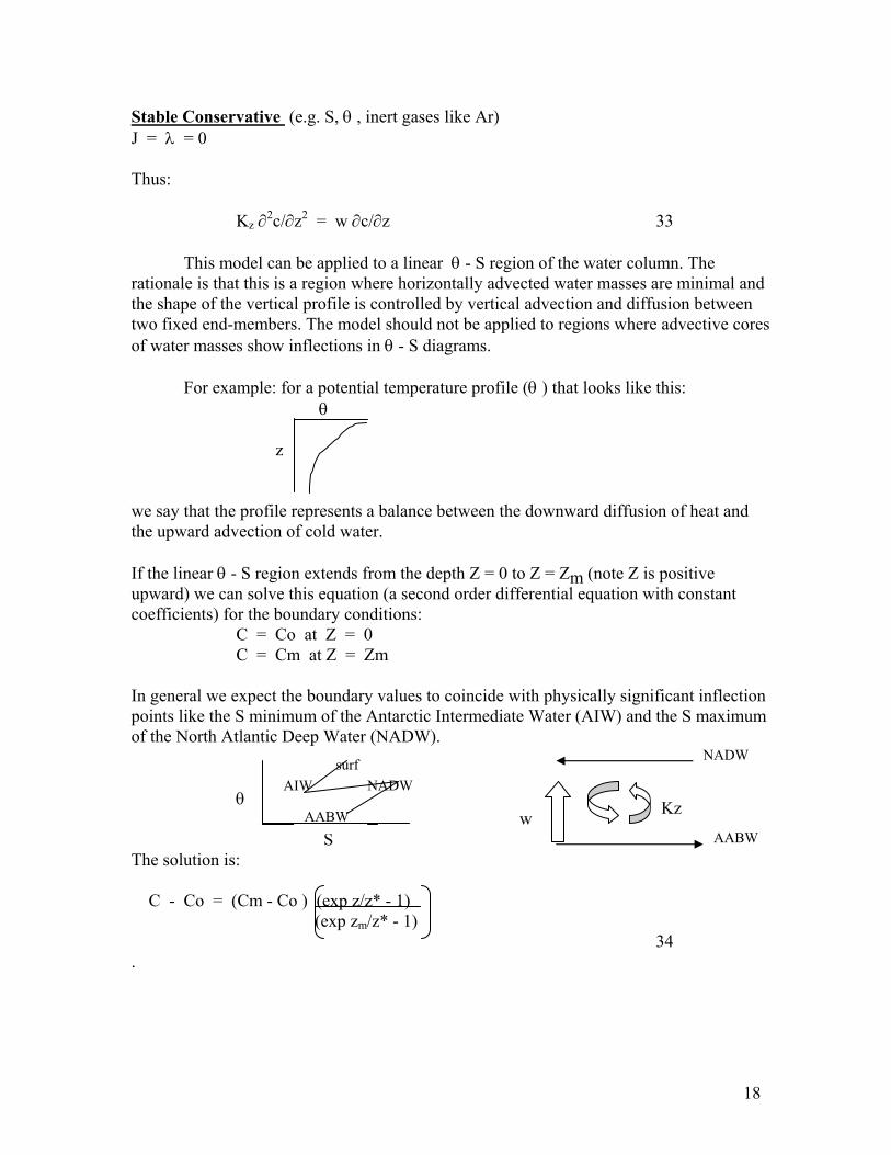
Stable Conservative (e.g. S, θ , inert gases like Ar) J = λ = 0 Thus: Kz ∂2c/∂z2 = w ∂c/∂z 33 This model can be applied to a linear θ - S region of the water column. The rationale is that this is a region where horizontally advected water masses are minimal and the shape of the vertical profile is controlled by vertical advection and diffusion between two fixed end-members. The model should not be applied to regions where advective cores of water masses show inflections in θ - S diagrams. For example: for a potential temperature profile (θ ) that looks like this: θ z we say that the profile represents a balance between the downward diffusion of heat and the upward advection of cold water. If the linear θ - S region extends from the depth Z = 0 to Z = Zm (note Z is positive upward) we can solve this equation (a second order differential equation with constant coefficients) for the boundary conditions: C = Co at Z = 0 C = Cm at Z = Zm In general we expect the boundary values to coincide with physically significant inflection points like the S minimum of the Antarctic Intermediate Water (AIW) and the S maximum of the North Atlantic Deep Water (NADW). θ S The solution is: C - Co = (Cm - Co ) (exp z/z* - 1) (exp zm/z* - 1) 34 .

surf AIW

AABW

NADW

NADW

AABW w Kz

19

where Z = positive upward (see figure) Zm = mixing interval Z* = Kz / w the ratio of the eddy diffusion coefficient / advection

velocity which is assumed to be constant with depth. The units for Z* are length (e.g. km) thus this parameter has been called the reciprocal scale length. A typical value for the deep ocean is about 1 km

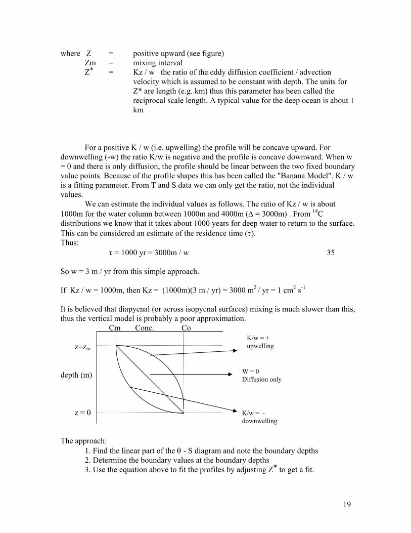
For a positive K / w (i.e. upwelling) the profile will be concave upward. For downwelling (-w) the ratio K/w is negative and the profile is concave downward. When w = 0 and there is only diffusion, the profile should be linear between the two fixed boundary value points. Because of the profile shapes this has been called the "Banana Model". K / w is a fitting parameter. From T and S data we can only get the ratio, not the individual values. We can estimate the individual values as follows. The ratio of Kz / w is about 1000m for the water column between 1000m and 4000m (∆ = 3000m) . From 14C distributions we know that it takes about 1000 years for deep water to return to the surface. This can be considered an estimate of the residence time (τ). Thus: τ = 1000 yr = 3000m / w 35 So w = 3 m / yr from this simple approach. If Kz / w = 1000m, then Kz = (1000m)(3 m / yr) = 3000 m2 / yr = 1 cm2 s-1 It is believed that diapycnal (or across isopycnal surfaces) mixing is much slower than this, thus the vertical model is probably a poor approximation. Cm Conc. Co z=zm depth (m) z = 0 The approach: 1. Find the linear part of the θ - S diagram and note the boundary depths 2. Determine the boundary values at the boundary depths 3. Use the equation above to fit the profiles by adjusting Z* to get a fit.

K/w = + upwelling

K/w = - downwelling

W = 0 Diffusion only

20

An example of the application of this model to θ - S data from the western North Pacific (28N ; 121W) is shown in the attached figure. The θ- S profile is linear from about 850m to 4160m. The value of Z* required to fit the θ profile is 0.875 km. That for S was 0.856 km. As both θ and S are conservative we expect them to be described by the same value of Kz / w . In addition, the same value of Kz implies that Kz must be about 100 times greater than Dheat. According to this logic the lower limit for Kz in the ocean is assumed to be about 0.1 cm2 sec-1.

21

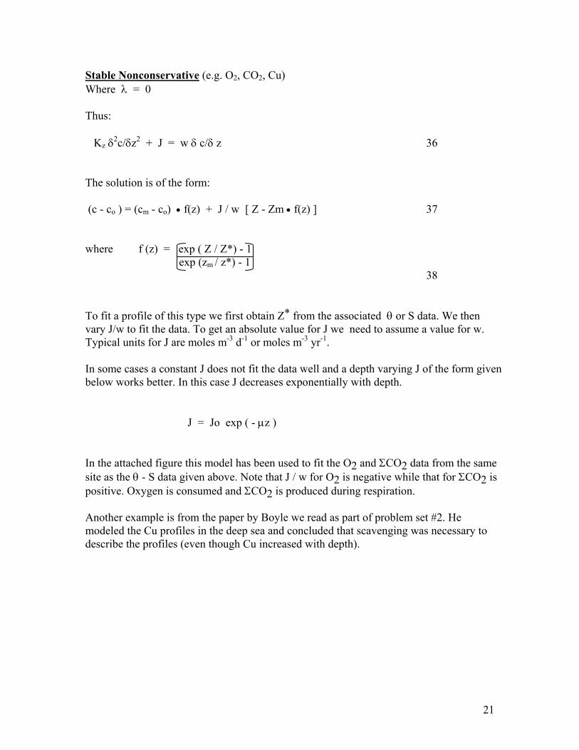
Stable Nonconservative (e.g. O2, CO2, Cu) Where λ = 0 Thus: Kz δ2c/δz2 + J = w δ c/δ z 36 The solution is of the form: (c - co ) = (cm - co) • f(z) + J / w [ Z - Zm • f(z) ] 37 where f (z) = exp ( Z / Z*) - 1 exp (zm / z*) - 1 38 To fit a profile of this type we first obtain Z* from the associated θ or S data. We then vary J/w to fit the data. To get an absolute value for J we need to assume a value for w. Typical units for J are moles m-3 d-1 or moles m-3 yr-1. In some cases a constant J does not fit the data well and a depth varying J of the form given below works better. In this case J decreases exponentially with depth. J = Jo exp ( - µz ) In the attached figure this model has been used to fit the O2 and ΣCO2 data from the same site as the θ - S data given above. Note that J / w for O2 is negative while that for ΣCO2 is positive. Oxygen is consumed and ΣCO2 is produced during respiration. Another example is from the paper by Boyle we read as part of problem set #2. He modeled the Cu profiles in the deep sea and concluded that scavenging was necessary to describe the profiles (even though Cu increased with depth).

22

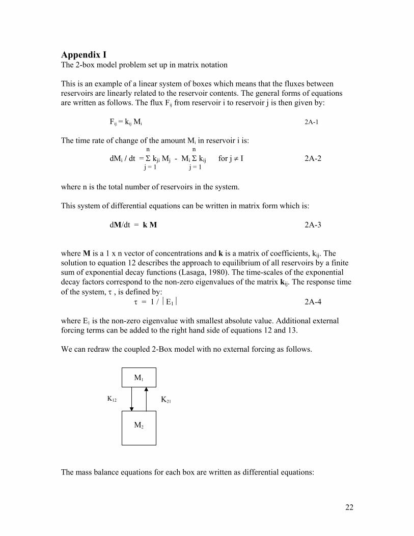
Appendix I The 2-box model problem set up in matrix notation This is an example of a linear system of boxes which means that the fluxes between reservoirs are linearly related to the reservoir contents. The general forms of equations are written as follows. The flux Fij from reservoir i to reservoir j is then given by: Fij = kij Mi 2A-1 The time rate of change of the amount Mi in reservoir i is: n n

dMi / dt = Σ kji Mj - Mi Σ kij for j ≠ I 2A-2 j = 1 j = 1

where n is the total number of reservoirs in the system. This system of differential equations can be written in matrix form which is: dM/dt = k M 2A-3 where M is a 1 x n vector of concentrations and k is a matrix of coefficients, kij. The solution to equation 12 describes the approach to equilibrium of all reservoirs by a finite sum of exponential decay functions (Lasaga, 1980). The time-scales of the exponential decay factors correspond to the non-zero eigenvalues of the matrix kij. The response time of the system, τ , is defined by:

τ = 1 / E1 2A-4

where E1 is the non-zero eigenvalue with smallest absolute value. Additional external forcing terms can be added to the right hand side of equations 12 and 13. We can redraw the coupled 2-Box model with no external forcing as follows. M1 M2 The mass balance equations for each box are written as differential equations:

K12 K21

23

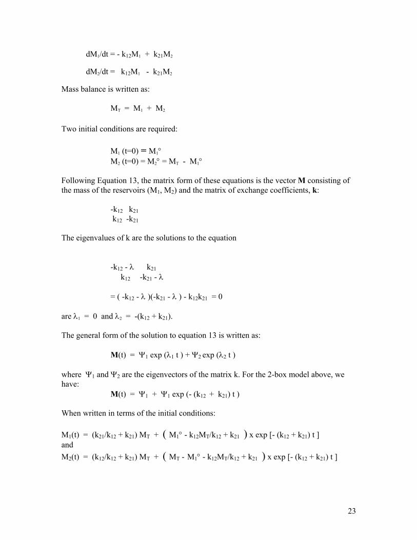
dM1/dt = - k12M1 + k21M2 dM2/dt = k12M1 - k21M2 Mass balance is written as: MT = M1 + M2 Two initial conditions are required: M1 (t=0) = M1° M2 (t=0) = M2° = MT - M1° Following Equation 13, the matrix form of these equations is the vector M consisting of the mass of the reservoirs (M1, M2) and the matrix of exchange coefficients, k: -k12 k21

k12 -k21 The eigenvalues of k are the solutions to the equation -k12 - λ k21 k12 -k21 - λ = ( -k12 - λ )(-k21 - λ ) - k12k21 = 0 are λ1 = 0 and λ2 = -(k12 + k21). The general form of the solution to equation 13 is written as: M(t) = Ψ1 exp (λ1 t ) + Ψ2 exp (λ2 t ) where Ψ1 and Ψ2 are the eigenvectors of the matrix k. For the 2-box model above, we have: M(t) = Ψ1 + Ψ1 exp (- (k12 + k21) t ) When written in terms of the initial conditions: M1(t) = (k21/k12 + k21) MT + ( M1° - k12MT/k12 + k21 ) x exp [- (k12 + k21) t ] and M2(t) = (k12/k12 + k21) MT + ( MT - M1° - k12MT/k12 + k21 ) x exp [- (k12 + k21) t ]

24

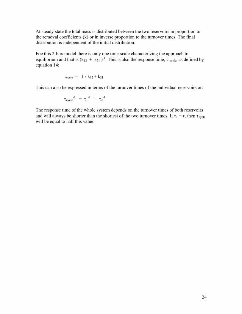
At steady state the total mass is distributed between the two reservoirs in proportion to the removal coefficients (k) or in inverse proportion to the turnover times. The final distribution is independent of the initial distribution. Foe this 2-box model there is only one time-scale characterizing the approach to equilibrium and that is (k12 + k21 )-1. This is also the response time, τ cycle, as defined by equation 14: τcycle = 1 / k12 + k21 This can also be expressed in terms of the turnover times of the individual reservoirs or: τcycle

-1 = τ1-1 + τ2

-1 The response time of the whole system depends on the turnover times of both reservoirs and will always be shorter than the shortest of the two turnover times. If τ1 = τ2 then τcycle will be equal to half this value.

25

References: Chameides W.L. and E.M. Perdue (1997) Biogeochemical Cycles. Oxford, 224 pp. Holland H.D. (1978) The Chemistry of the Atmosphere and Ocean. Wiley-Interscience. 351 pp. Lasaga A.C. (1981) Dynamic Treatment of Geochemical Cycles: Global Kinetics. In: (A.C. Lasaga and R.J. Kirkpatrick, eds) Kinetics of Geochemical Processes. Vol. 8. Reviews in Mineralogy. Min. Soc. Am., 69-110. Lasaga A.C. (1980) The kinetic treatment of geochemical cycles. Geochim. Cosmochim. Acta, 44, 815-828. Li Y-H (1977) Confusion of the mathematical notation for defining the residence time. Geochim. Cosmochim. Acta, 41, 555-556. Platt J.R. (1964) Strong Inference. Science, 146, 347-353. Prigogine I. (1967) Introduction to Thermodynamics of Irreversible Processes. Wiley-Interscience, 147pp. Rodhe H. (1992) Modeling Biogeochemical Cycles. In: (S.S. Butcher, R.J. Charlson. G.H. Orians and G.V. Wolfe, eds.) Global Biogeochemical Cycles. Academic Press. 55-72. Safire W. (1999) Ockham's Razor's Close Shave. The New York Times Magazine, Jan. 31, 1999. p.14.

26

Problems: 2-1: Dynamic Box Model Consider a beaker of distilled water with a constant volume and constant water inflow and outflow. If the concentration of an element in the inflow is suddenly changed how would the concentration in the beaker change with time? V = water volume (cm3) C = concentration (moles cm-3) Cin = inflow concentration F = flow rate (cm3 s-1) 2-2 Box Models - Red Sea What is the effect of river water diversion on the water balance of marginal seas and other seas with limited connection to the oceans? Lets look at the Red Sea as an example to test a hypothetical situation (but some of these numbers are made up). The surrounding nations of Egypt, Sudan, Eritrea and Saudia Arabia are intent on exploiting all sources of water for irrigation. Current runoff to the Red Sea (rivers + groundwater) is 0.5 m/y. Direct precipitation to the surface is 0.25 m/y and evaporation is 2.0 m/yr; both remain unchanged. Some amount of seawater enters the Arabian Sea through the strait of Bab el Mandeb, but the total volume of the Red Sea is at steady state. The surface area is 0.5 x 106 km2 and the total volume of water is 0.25 x 106 km3. a. Draw a sketch box model of the present situation. Label all the fluxes. b. Write the mass balance equation for water at steady state. c. Calculate the residence time of water in the Red Sea with respect to Arabian Sea input. d. The total effect of the river diversion project is to reduce total runoff to 10% of its current value. Calculate the new flux of water from the Arabian Sea and the new residence time of the Red Sea with respect to Arabian Sea inflow. 2-3. Box Models - Black Sea The Black Sea is a permanent anoxic basin. Its average depth is about 2000m. The only source of salt water is from the Mediterranean through the Bosporus (QB). Many freshwater rivers ( with S = 0 ) including the Danube drain into the surface layer (QR). As the seawater enters through the Bosporus it entrains surface water (QE) (with S = 18.5) to form Black Sea deep water (QD) with S = 22.33. The deep water ultimately upwells into the surface layer. The box model shown below has been proposed to describe this process (Murray et al, 1991, Deep-Sea Research, 38, 663-690). a. Write the mass balance for water in the deep box. b. Write the mass balance for salt in the deep box. c. What is the rate of entrainment (QE) that is required to form the deep water if: SB = 35.0 ; SE = 18.5 ; SD = 22.33 and QB = 3.12 x 102 km3 y-1 What is the QE/QB ratio? d. The volume of the deep water of the Black Sea is 5.20 x 1017 l. Define and calculate its residence time.

27

2-4 From McDuff and Morel (1980) There is 1.3 x 109 Tg S as SO4 in the ocean. The river source today is 100 TgS y-1 and the hydrothermal sink is also equal to 100 TgS y-1. If the river source suddenly increased to 200 TgS y-1, what would be the final steady state value and how long would it take to reach it?