Chapter 2 Lorentz contraction from the classical wave...

Chapter 2

Lorentz contraction from the classical wave

equation

−from my book:

Understanding Relativistic Quantum Field Theory

Hans de Vries

July 30, 2008

2 Chapter

Contents

2 Lorentz contraction from the classical wave equation 12.1 Moving solutions of the classical wave equation . . . . . . 22.2 The Lienard Wiechert potentials . . . . . . . . . . . . . . 32.3 The Lorentz contracted EM potentials . . . . . . . . . . . 62.4 The Lorentz transform of the EM potentials . . . . . . . . 72.5 The Lorentz transform of charge and current . . . . . . . 92.6 The Lorentz contracted E and B fields . . . . . . . . . . . 112.7 Lorentz transform of the E and B fields . . . . . . . . . . 132.8 The Lienard Wiechert E and B fields . . . . . . . . . . . . 162.9 The phantom location of a moving charge . . . . . . . . . 172.10 Derivation of the Lienard Wiechert E field . . . . . . . . . 182.11 Derivation of the Lienard Wiechert B field . . . . . . . . . 212.12 Point charge radiation fields from acceleration . . . . . . . 22

Chapter 2

Lorentz contraction from theclassical wave equation

...

2 Chapter 2. Lorentz contraction from the classical wave equation

2.1 Moving solutions of the classical wave equation

We turn our attention again to the classical wave equation. This time tolook at solutions which are moving with a constant speed v, say for instancein the x-direction. An arbitrary function which shifts along with a speedv in the x direction does satisfy equations which relates the derivatives int and x by the speed v in the following way:

∂Φ∂t

= −v∂Φ∂x

∂2Φ∂t2

= v2∂2Φ∂x2

(2.1)

These equations are valid for any arbitrary potential function Φ. We cancombine the latter in the the the classical wave equation for three spatialdimensions.

∂2Φ∂t2

− c2∂2Φ∂x2

− c2∂2Φ∂y2

− c2∂2Φ∂z2

= 0 (2.2)

and use it to replace the 2nd order time derivative with the 2nd orderx-derivative in order to eliminate the time dependency. We get:(

1− v2

c2

)c2∂2Φ∂x2

+ c2∂2Φ∂y2

+ c2∂2Φ∂z2

= 0 (2.3)

This shows that the solutions are Lorentz contracted in the direction of vby a factor γ, The first order derivatives are higher by a factor γ and thesecond order by a factor γ2. Velocities higher then c are not possible. Thisproof can’t hardly be any simpler, however we want to study this in somemore detail by using the 3d-propagator.

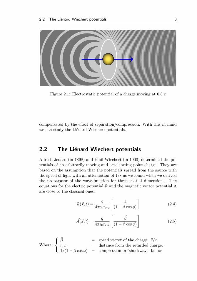
Figure 2.1 shows how the field Φ propagates away from the charge spher-ically while decreasing in amplitude 1/r. Thicker circles depict a higheramplitude. The field behind the charge was emitted more recently, the”circles” have a higher amplitude but are further separated. The field infront of the charge was emitted longer ago, the circles have a lower ampli-tude but they are compressed closer together.

Since the Lorentz contracted field is mirror-symmetric in the x-axis, weconclude that the effect of the higher/lower amplitude apparently must be

2.2 The Lienard Wiechert potentials 3

Figure 2.1: Electrostatic potential of a charge moving at 0.8 c

compensated by the effect of separation/compression. With this in mindwe can study the Lienard Wiechert potentials.

2.2 The Lienard Wiechert potentials

Alfred Lienard (in 1898) and Emil Wiechert (in 1900) determined the po-tentials of an arbitrarily moving and accelerating point charge. They arebased on the assumption that the potentials spread from the source withthe speed of light with an attenuation of 1/r as we found when we derivedthe propagator of the wave-function for three spatial dimensions. Theequations for the electric potential Φ and the magnetic vector potential Aare close to the classical ones:

Φ(~x, t) =q

4πε0rret

[1

(1− β cosφ)

](2.4)

~A(~x, t) =q

4πε0rret

[~β

(1− β cosφ)

](2.5)

Where:

~β = speed vector of the charge: ~v/crret = distance from the retarded charge.1/(1− β cosφ) = compression or ’shockwave’ factor


Note that the equations use the retarded charge location: The locationwhere the charge was at the moment when the potentials were emittedfrom the point charge. From the formula’s we see that all the informationthat is needed is:

(1) the charge, (2) its location, and (3) its speed.

We have this information if we know the position of the point charge attwo different moments in time, at t and at t+dt. The value of Φ at a singlepoint in space-time (t,r) therefor doesn’t contain any information aboutthe acceleration of the charge, it only depends on position and speed. Thisis unlike the equations for the E and B fields which do in fact depend onthe acceleration, because they are based on the derivatives of the potentialfields.

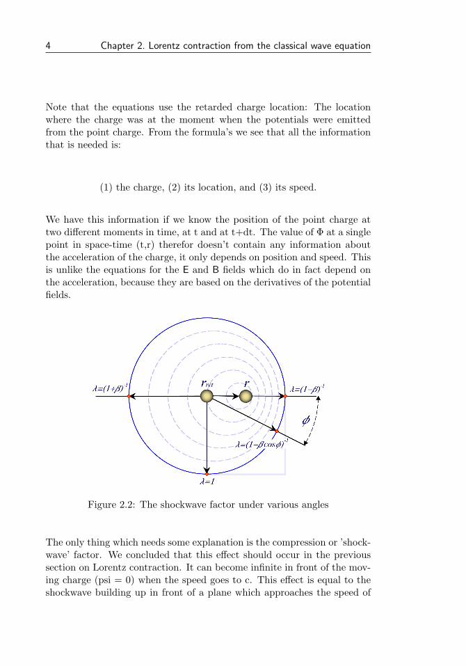
Figure 2.2: The shockwave factor under various angles

The only thing which needs some explanation is the compression or ’shock-wave’ factor. We concluded that this effect should occur in the previoussection on Lorentz contraction. It can become infinite in front of the mov-ing charge (psi = 0) when the speed goes to c. This effect is equal to theshockwave building up in front of a plane which approaches the speed of

2.2 The Lienard Wiechert potentials 5

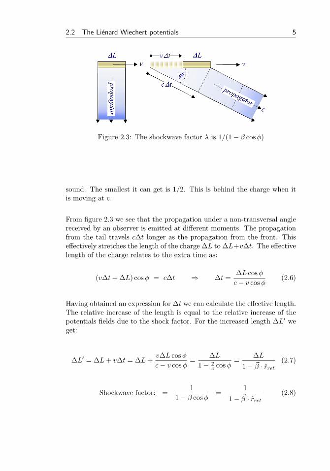
Figure 2.3: The shockwave factor λ is 1/(1− β cosφ)

sound. The smallest it can get is 1/2. This is behind the charge when itis moving at c.

From figure 2.3 we see that the propagation under a non-transversal anglereceived by an observer is emitted at different moments. The propagationfrom the tail travels c∆t longer as the propagation from the front. Thiseffectively stretches the length of the charge ∆L to ∆L+v∆t. The effectivelength of the charge relates to the extra time as:

(v∆t+ ∆L) cosφ = c∆t ⇒ ∆t =∆L cosφc− v cosφ

(2.6)

Having obtained an expression for ∆t we can calculate the effective length.The relative increase of the length is equal to the relative increase of thepotentials fields due to the shock factor. For the increased length ∆L′ weget:

∆L′ = ∆L+ v∆t = ∆L+v∆L cosφc− v cosφ

=∆L

1− vc cosφ

=∆L

1− ~β · rret(2.7)

Shockwave factor: =1

1− β cosφ=

1

1− ~β · rret(2.8)


2.3 The Lorentz contracted EM potentials

To obtain the Lorentz contracted fields from the Lienard Wiechert poten-tials we need to rewrite them with the respect to the current location ofthe charge instead of the retarded using the fact that the velocity is nowconstant. If we locate the current position at the origin then we can derivethe distance from any point (x, y, z) to the retarded location and the angleφ belonging to that location.

rret =√

(x+ vt)2 + y2 + z2, cosφ =(x+ vt)√

(x+ vt)2 + y2 + z2(2.9)

Checking this from positions on the three principle axis we find for theLorentz contracted potential.

(x, 0, 0) ⇒ rret = x/(1− β), cosφ = ±1(0, y, 0) ⇒ rret = γ y, cosφ = β(0, 0, z) ⇒ rret = γ z, cosφ = β

(2.10)

giving the potential fields on the principle axis:

Φ(x, 0, 0) =q

4πε0x, ~A(x, 0, 0) =

~β q/c

4πε0x(2.11)

Φ(0, y, 0) =γ q

4πε0y, ~A(0, y, 0) =

γ~β q/c

4πε0y(2.12)

Φ(0, 0, z) =γ q

4πε0z, ~A(0, 0, z) =

γ~β q/c

4πε0z(2.13)

The general expressions for the Lorentz contracted potentials for a chargemoving on the x-axis:

Φ(x, y, z) =γ q

4πε0√

(γx)2 + y2 + z2(2.14)

~A(x, y, z) =γ ~β q/c

4πε0√

(γx)2 + y2 + z2(2.15)

2.4 The Lorentz transform of the EM potentials 7

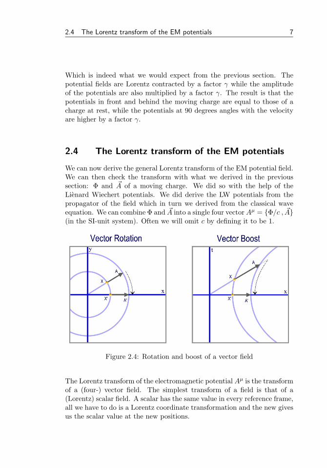
Which is indeed what we would expect from the previous section. Thepotential fields are Lorentz contracted by a factor γ while the amplitudeof the potentials are also multiplied by a factor γ. The result is that thepotentials in front and behind the moving charge are equal to those of acharge at rest, while the potentials at 90 degrees angles with the velocityare higher by a factor γ.

2.4 The Lorentz transform of the EM potentials

We can now derive the general Lorentz transform of the EM potential field.We can then check the transform with what we derived in the previoussection: Φ and ~A of a moving charge. We did so with the help of theLienard Wiechert potentials. We did derive the LW potentials from thepropagator of the field which in turn we derived from the classical waveequation. We can combine Φ and ~A into a single four vector Aµ = {Φ/c , ~A}(in the SI-unit system). Often we will omit c by defining it to be 1.

Figure 2.4: Rotation and boost of a vector field

The Lorentz transform of the electromagnetic potential Aµ is the transformof a (four-) vector field. The simplest transform of a field is that of a(Lorentz) scalar field. A scalar has the same value in every reference frame,all we have to do is a Lorentz coordinate transformation and the new givesus the scalar value at the new positions.


In case of a vector field we also need to transform the vector itself as shownin figure 2.4. In this case we can simply treat the four vector Aµ as thefour vector xµ. The standard Lorentz coordinate transform (with c = 1)is given by.

forward transform backward transform

t′ = γ(t − ~β · ~x

)t = γ

(t′ + ~β · ~x′

)~x′‖ = γ

(~x‖ − ~β t

)~x‖ = γ

(~x′‖ + ~β t′

)~x′⊥ = ~x⊥ ~x⊥ = ~x′⊥

(2.16)

Where we have split ~x into ~x‖+~x⊥, the components parallel and orthogonalto the boost β. We now simply replace xµ with Aµ to obtain the Lorentztransform of the potential field.

Lorentz transformation of the electromagnetic four-vector Aµ


Φ′ = γ(

Φ − ~β · ~A)

Φ = γ(

Φ′ + ~β · ~A′)

~A′‖ = γ(~A‖ − ~β Φ

)~A‖ = γ

(~A′‖ + ~β Φ′

)~A′⊥ = ~A⊥ ~A⊥ = ~A′⊥

(2.17)

Where we have used c=1 (for full SI replace Φ by Φ/c). The parallel andorthogonal components can be given as vector expressions involving theunit-vector β in the direction of the boost.

~A‖ = ( β · ~A ) β parallel component with regard to ~β

~A⊥ = ( β × ~A )× β orthogonal component with regard to ~β(2.18)

2.5 The Lorentz transform of charge and current 9

In the simple case of a transformation from the rest-frame of the sourcecharge of the field to a boosted frame we can write.(

Φ/c, ~A)

transforms like(γ, ~βγ

)(2.19)

We see this back in the general expressions for the Lorentz contractedpotentials for a charge moving on the x-axis which we derived in section2.3.

Φ(x, y, z) =γ q

4πε0√

(γx)2 + y2 + z2(2.20)

~A(x, y, z) =γ ~β q/c

4πε0√

(γx)2 + y2 + z2(2.21)

The changes x → γx are the result of the Lorentz contraction (the co-ordinate transformation) while the factors γ and ~βγ are the result of thetransformation of the transformation of the four-vector Aµ.

2.5 The Lorentz transform of charge and current

Since the electromagnetic potential Aµ has as its source the charge/currentdensity jµ = { ρ ,~j } we may expect that Aµ and jµ transform in the sameway.

Lorentz transformation of the charge-current density jµ


ρ′ = γ(ρ − ~β ·~j

)ρ = γ

(ρ′ + ~β ·~j′

)~j′‖ = γ

(~j‖ − ~β ρ

)~j‖ = γ

(~j′‖ + ~β ρ′

)~j′⊥ = ~j⊥ ~j⊥ = ~j′⊥

(2.22)

Where the parallel and orthogonal components of ~j relative to the boostare given by.


~j‖ = ( β · ~j ) β parallel component with regard to ~β

~j⊥ = ( β ×~j )× β orthogonal component with regard to ~β(2.23)

A charge density at rest transforms into a charge/current density as.(ρ , ~j

)transforms like

(γ , ~βγ

)(2.24)

The total charge Q and total current ~J

For sofar we have discussed the transformation of the charge and currentdensities. The total charge and total current are obtained by integratingover space. The space over which the charge/current is spread reduces by afactor gamma, with the result that the total charge and current transformless by a factor γ, thus.(

Q , ~J)

transforms like(

1 , ~β)

(2.25)

This is a fundamental result. It means that the charge is reference frameindependent. The current is always proportional to the speed. This incontrast with the energy/momentum of a particle which transforms as weknow like. (

E , ~p

)transforms like

(γ , ~βγ

)(2.26)

Again we encounter something truly fundamental here. The energy/ mo-mentum of a particle determines its resistance to the change of motion dueto a force exerted on the particle. The electromagnetic force is determinedby the value of the charge Q2, which in contrast to the ”relativistic mass”γmc2 does not transform.

The difference of the factor γ in the way which E and Q2 transform nowleads to the effect of time dilatation whereby all processes proceed slowerby a factor γ. We will discuss this subject in more detail in chapter ??:”Time dilation from the classical wave equation”.

2.6 The Lorentz contracted E and B fields 11

2.6 The Lorentz contracted E and B fields

We want to derive the E and B fields of a moving electric charge. This isstraightforwardly done by using Maxwell’s laws to obtain the field from thepotentials Φ and ~A. The general expressions for the Lorentz contractedpotentials for a charge moving on the x-axis are:

Φ(x, y, z) =γ q

4πε0√

(γx)2 + y2 + z2(2.27)

~A(x, y, z) =γ ~β q/c

4πε0√

(γx)2 + y2 + z2(2.28)

Where ~β = { βx , 0 , 0 } is along the x-axis. The E and B fields arederived from the potentials by.

E = −grad Φ− ∂ ~A

∂t(2.29)

B = curl ~A (2.30)

When written out in full these give us.

E ={−∂Φ∂x− ∂Ax

∂t, − ∂Φ

∂y− ∂Ay

∂t, − ∂Φ

∂z− ∂Az

∂t

}(2.31)

B ={

∂Az∂y− ∂Ay

∂z,

∂Ax∂z− ∂Az

∂x,

∂Ay∂x− ∂Ax

∂y

}(2.32)

The magnetic vector potential components Ay and Az are zero while Axhas a simple relation with the potential Φ:

Ax = βxΦ (2.33)

We can change a derivative in t to derivative in x by simply multiplyingit with −βx since our solution shifts in the x-direction with a speed vx, sowe have:

∂Ax∂t

= −βx∂Ax∂x

= −β2x

∂Φ∂x

, thus: (2.34)


Ex = −∂Φ∂x− ∂Ax

∂t= −(1− β2

x)∂Φ∂x

(2.35)

This gives us for the Ex component of the electric field.

Ex =(1− β2

x) γ3x q

4πεo(γ2x2 + y2 + z2)3/2(2.36)

Ex =γ x q

4πεo(γ2x2 + y2 + z2)3/2(2.37)

The Ey and Ez components are simpler since Ay = Az = 0. These com-ponents of the electric field become.

Ey =γ y q

4πεo(γ2x2 + y2 + z2)3/2, Ez =

γ z q

4πεo(γ2x2 + y2 + z2)3/2(2.38)

We see that the factor (1− β2x) was canceled by the extra factor γ2 due to

the differentiation along the (Lorentz contracted) x-axis. All nominatorshave a similar form now so we can simply write this in vector form.

Electric field E of a moving charge

E =γ ~r q

4πεo(γ2x2 + y2 + z2)3/2(2.39)

When we derive the magnetic field B we see that the the E field and theB field relate to each other in a simple way.

E = −~v × B, B =~v

c2× E (2.40)

So here we can obtain the magnetic field B simple from the electric field.

Magnetic field B of a moving charge

B =γ(~β × ~r

)q/c

4πεo(γ2x2 + y2 + z2)3/2(2.41)

2.7 Lorentz transform of the E and B fields 13

Relation 2.40 holds for an arbitrary moving monopole point source. In thelimit cases for β = 0 we retrieve the standard static fields.

limβ→0

E =~r q

4πεor3, lim

β→0B =

~β × ~r q/c4πεor3

(2.42)

We can represent these expressions in spherical coordinates with the helpof the replacement sin2 θ = (y2 + z2)/(x2 + y2 + z2)

E =~r q

4πεo r3γ2(1− β2 sin2 θ)3/2(2.43)

B =

(~β × ~r

)q/c

4πεo r3γ2(1− β2 sin2 θ)3/2(2.44)

2.7 Lorentz transform of the E and B fields

In the previous section we made use of a relation between the electric andmagnetic fields of a moving (monopole) charge.

E = −~v × B, B =~v

c2× E (2.45)

We can prove this easily for a constant speed v with the help of the genericexpressions.

E = −grad Φ− ∂ ~A

∂t, B = curl ~A (2.46)

Substitution gives us for the magnetic field.

B = curl ~A = − ~v

c2× grad Φ − ~v

c2× ∂ ~A

∂t(2.47)

The last term with the time derivative is zero if the speed v is constantdue to the relation ~A = Φ~v/c2. The vector potential ~A points always inthe direction of ~v, so a change of ~A is also in the direction of ~v and thecross product is always zero.


~v

c2× ∂ ~A

∂t= 0 (2.48)

Without this term and after replacing ~A with Φ~v/c2 the remaining expres-sion becomes.

B =1c2∇× (Φ~v) =

1c2∇(Φ) × ~v (2.49)

Which is true due to the chain rule and ∇ × ~v = 0. in the situation ofan arbitrary charge/current density distribution this relation between Eand B obviously doesn’t hold, however, it does appears in the Lorentztransform of the electromagnetic field.

In the case of the Lorentz transform of the EM-field under a (constant)boost in velocity the relations (2.77) determine how the electric and mag-netic field are transformed into each other. For instance in the case of aboost in the x-direction.

E′x = Ex B′x = BxE′y = γ(Ey − vBz) B′y = γ(By + v

c2Ez)

E′z = γ(Ez + vBy) B′z = γ(Bz − vc2Ey)

(2.50)

Which we can rewrite for an arbitrary boost using a short hand notationfor the various components of the fields parallel and orthogonal with regardto the boost ~β and further simplified by setting c to 1.

Lorentz transform of the electromagnetic field

E′ = E‖ + E⊥ γ + B⊗ βγB′ = B‖ + B⊥ γ − E⊗ βγ

(2.51)

E‖ = ( β · E ) β parallel component with regard to ~β

E⊥ = ( β × E )× β orthogonal component with regard to ~β

E⊗ = ( β × E ) 90o rotated orthogonal component(2.52)

2.7 Lorentz transform of the E and B fields 15

We can apply these transformation expressions on a moving point chargeand check if we get the same results as in the previous section. Firstwe have to apply a coordinate transform. We are only interested in t′=0where the particle is in the coordinate center. The fields of the particleare independent on time in the particles rest-frame. So, al we need to dois replacing x by γx which corresponds to the Lorentz contraction.

E =~r q

4πεor3⇒ ( γx x + y y + z z ) q

4πεo(γ2x2 + y2 + z2)3/2(2.53)

After the coordinate transformation we have to do the field transformation.The electromagnetic field transforms, in the way as given above, as an anti-symmetric tensor. which we will discuss in more detail in the chapter onthe relativistic formulation of fields.

From the Field transform equations (2.51) we see that the componentsorthogonal to the boost acquire an extra factor γ while the componentparallel to the boost doesn’t. The total transformation, coordinate plusfield transformation thus yields:

E =~r q

4πεor3⇒ γ~r q

4πεo(γ2x2 + y2 + z2)3/2(2.54)

Which corresponds to expression (2.39) which we derived in the previoussection. Now we want to obtain the magnetic field of a moving charge fromthe general Lorentz transform of the magnetic field. In the rest frame thereis no magnetic field but we have to transform the rest-frames E field intoa magnetic field.

First step is again the coordinate transform of the E-field as in (2.53)after which comes the field transform. This involves a cross-product ~β×Ewhich uses only the components orthogonal of E in (2.53) removing theterm γx x. The result we get corresponds with the magnetic field of amoving charge which we derived in (2.41).

B =γ(~β × ~r

)q/c

4πεo(γ2x2 + y2 + z2)3/2(2.55)


2.8 The Lienard Wiechert E and B fields

It is important to realize that the potentials Φ and A are propagating onthe light cone and the electric and magnetic fields E and B are derivativefields. If we would rewrite the formula’s for the E and B fields in the sameway using the retarded location and a shockwave factor then we obtain in-correct expressions, which would for instance not show any electromagneticradiation.

We do however get the EM fields by carefully differentiating the potentialsin space and time. Carefully because we use retarded values in our for-mula’s for Φ and A to obtain current values. Before we proceed into thiswe’ll first have a look at the results:

E(~x, t) =q

4πε0r2ret

[(1− β2) ~rph

(1− β cosφ)3

]+

q

4πε0rret

[rret × (~rph × ~a)c2(1− β cosφ)3

](2.56)

B(~x, t) =rretc× E (2.57)

where:

~a = accelaration vector of the charge.rret = unit vector from retarded charge towards (~x, t)~rph = vector (rret − ~β) from phantom location to (~x, t)

with v � c this simplifies to:

E(~x, t) =q

4πε0r2r − q

4πε0r1c2

r × (r × ~a) (2.58)

We see that the first term is the standard Coulomb field. The secondterm is the radiation term which is proportional to the acceleration of thecharge. The radiation term decreases with only 1/r rather than with 1/r2

as the Coulomb field does. This leads to a finite energy flux (E × B)/µoaway from the charge at any r →∞.

A constant amount of energy has to be fed to the charge to keep it ra-diating. This in contrast with the energy associated with the Coulombfield. If we could ”create” a charge, (which we can’t because charge is aconserved quantity), then the amount of energy we would need to buildup the Coulomb field would decrease by 1/t2 and reach some maximum inthe limit case of t going to infinity.

2.9 The phantom location of a moving charge 17

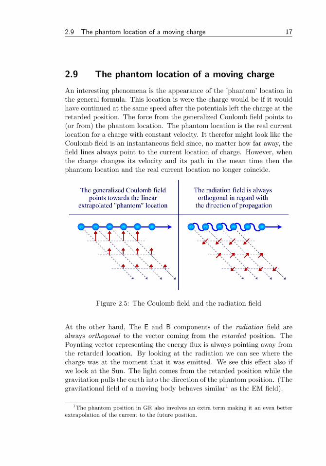
2.9 The phantom location of a moving charge

An interesting phenomena is the appearance of the ’phantom’ location inthe general formula. This location is were the charge would be if it wouldhave continued at the same speed after the potentials left the charge at theretarded position. The force from the generalized Coulomb field points to(or from) the phantom location. The phantom location is the real currentlocation for a charge with constant velocity. It therefor might look like theCoulomb field is an instantaneous field since, no matter how far away, thefield lines always point to the current location of charge. However, whenthe charge changes its velocity and its path in the mean time then thephantom location and the real current location no longer coincide.

Figure 2.5: The Coulomb field and the radiation field

At the other hand, The E and B components of the radiation field arealways orthogonal to the vector coming from the retarded position. ThePoynting vector representing the energy flux is always pointing away fromthe retarded location. By looking at the radiation we can see where thecharge was at the moment that it was emitted. We see this effect also ifwe look at the Sun. The light comes from the retarded position while thegravitation pulls the earth into the direction of the phantom position. (Thegravitational field of a moving body behaves similar1 as the EM field).

1The phantom position in GR also involves an extra term making it an even betterextrapolation of the current to the future position.


2.10 Derivation of the Lienard Wiechert E field

To derive the electric field E and the magnetic field B from the LienardWiechert potentials we have to apply the standard formulas.

E = −∇Φ− 1c

∂ ~A

∂t, B = ∇× ~A (2.59)

However, we express the Lienard Wiechert potentials, and subsequentlythe E and B fields, using retarded values, like the distance, speed, andacceleration, that the charge had at the moment when the potentials wereemitted.

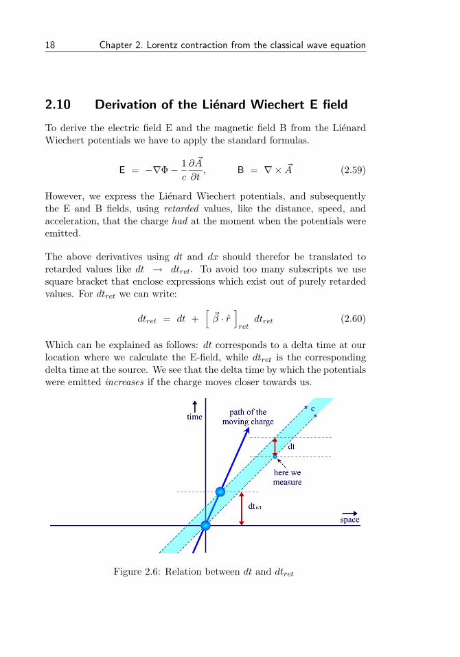
The above derivatives using dt and dx should therefor be translated toretarded values like dt → dtret. To avoid too many subscripts we usesquare bracket that enclose expressions which exist out of purely retardedvalues. For dtret we can write:

dtret = dt +[~β · r

]ret

dtret (2.60)

Which can be explained as follows: dt corresponds to a delta time at ourlocation where we calculate the E-field, while dtret is the correspondingdelta time at the source. We see that the delta time by which the potentialswere emitted increases if the charge moves closer towards us.

Figure 2.6: Relation between dt and dtret

2.10 Derivation of the Lienard Wiechert E field 19

It takes a longer time at the beginning of dtret to propagate from source tous as at the end of dtret since the charge has moved closer during the timedtret. We recover the shockwave factor if we write down the ratio betweenthe time deltas:

∂tret∂t

=[

1

1− ~β · r

]ret

(2.61)

We can now do the differentiation of an arbitrary function F in time byfirst differentiating at retarded time and then correcting the result via thechain rule.

∂Fret∂t

=∂Fret∂tret

∂tret∂t

=[

1

1− ~β · r

]ret

Fret (2.62)

We can do the same for the spatial derivatives. We go back to equation(2.60) and replace dt with a spatial derivative:

dtret = −1c

[~r · ~dxr

]ret

+[~β · r

]ret

dtret (2.63)

The first term on the right hand side now expresses the change in timeof the emission at the source when we shift our position of measurementover a distance dx. If the displacement of dx is orthogonal to ~r then thiscomponent of dtret becomes zero: The signal received at x and x+ dx wasemitted at the same time.

If the displacement along dx is parallel to ~r, then the time difference be-comes maximal and equal to the time needed to move over a distance ofdx at the speed of light. We can reorder (2.63) to express the ratio of dtretand dx:

∂tret∂x

= −1c

[~rx/r

(1− ~β · r)

]ret

(2.64)

We can use this relation to differentiate any arbitrary function F withregard to x by first differentiating at retarded time to dtret and use chainrule with the above result to get the derivative in x. Repeating this for yand z we can write.


∇ Fret = [ ∇F ]ret −1c

[r

1− ~β · r

]ret

Fret (2.65)

Using formulas (2.62) and (2.65) we can now derive the electric field E andthe magnetic field B from the Lienard Wiechert potentials. Using,

E = −∇Φ− 1c

∂ ~A

∂t(2.66)

Φ =q

4πε0

∣∣∣∣∣ 1

r (1− ~β · r )

∣∣∣∣∣ret

, ~A =q

4πε0

∣∣∣∣∣ ~β

r (1− ~β · r )

∣∣∣∣∣ret

(2.67)

We get the following expressions for the two terms making up E.

1c

∂ ~A

∂t=

q

4πεo

(β/c

r(1− ~β · r )2+−~β · r + (β/c) · ~r + β2

r2(1− ~β · r )3~β

)∣∣∣∣∣ret

(2.68)

∇Φ =q

4πεo

(r − ~β

r2(1− ~β · r )2− −

~β · r + (β/c) · ~r + β2

r2 (1− ~β · r )3r

)∣∣∣∣∣ret

(2.69)

Which can be simplified using the substitutions λ = 1/(1− ~β · r ) for theshockwave factor and ~rph = r− ~β for the vector pointing from the phantomposition to the measurement point.

1c

∂ ~A

∂t=

q

4πεor2(λ2(r/c)β + λ3

[(r/c)β · r − ~rph · ~β

]~β)∣∣∣∣ret

(2.70)

∇Φ =q

4πεor2(λ2 ~rph − λ3

[(r/c)β · r − ~rph · ~β

]r)∣∣∣∣ret

(2.71)

Where β is related to the acceleration and the velocity of the charge as~a/c2 = β/c = v/c2. The time derivative term (2.70) dependents mainlyon the acceleration of the charge. This was to be expected since ~A is pro-portional to the velocity of the charge. The second part of (2.70) dependson the velocity and can be neglected at lower charge velocity. We use astandard vector identity to collect various radiation terms together.

2.11 Derivation of the Lienard Wiechert B field 21

A× (B × C) = B (A · C) − C (A ·B) (2.72)

r × ( (r − ~β) × β ) = (r − ~β) (r · β) − β (1− ~β · r ) (2.73)

By doing so we arrive at the usual presentation of electric field from acharge with arbitrary motion and acceleration:

Electric field E of an arbitrary moving/accelarating charge

E =q

4πεor2

((1− β2) (r − ~β)

(1− ~β · r )3+

r

c

r × ( (r − ~β) × β )

(1− ~β · r )3

)∣∣∣∣∣ret(2.74)

We can simplify this expression as before by using ~rph = r − ~β which ispointing along the direction of the line from the phantom location to thepoint for which we calculate the field.

E =q

4πεor2

((1− β2) ~rph

(r · ~rph)3+

r

c

r × ( ~rph × β )(r · ~rph)3

)∣∣∣∣∣ret

(2.75)

Furthermore we can use the direction dependent shockwave factor λ =1/(1− ~β · r ) which can be interpreted as the ”compression” of the emittedpotential field in front of the charge due to its motion.

E =q

4πεor2λ3(

(1− β2) ~rph +r

cr × ( ~rph × β )

)∣∣∣∣ret

(2.76)

2.11 Derivation of the Lienard Wiechert B field

For the magnetic B field we need to take the curl∇× ~A of the magnetic vec-tor potential. Careful evaluation shows up that the electric and magneticfield are related to each other by.

B =rretc2× E (2.77)


Which gives us for the magnetic field of an arbitrary moving and acceler-ating charge:

Magnetic field B of an arbitrary moving/accelarating charge

B =q/c

4πεor2

((1− β2) r × (r − ~β)

(1− ~β · r )3+

r

c

r × (r × ( (r − ~β) × β ))

(1− ~β · r )3

)∣∣∣∣∣ret

(2.78)

2.12 Point charge radiation fields from acceleration

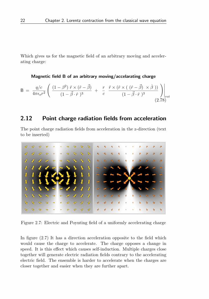
The point charge radiation fields from acceleration in the z-direction (textto be inserted)

Figure 2.7: Electric and Poynting field of a uniformly accelerating charge

In figure (2.7) It has a direction acceleration opposite to the field whichwould cause the charge to accelerate. The charge opposes a change inspeed. It is this effect which causes self-induction. Multiple charges closetogether will generate electric radiation fields contrary to the acceleratingelectric field. The ensemble is harder to accelerate when the charges arecloser together and easier when they are further apart.

2.12 Point charge radiation fields from acceleration 23

Eacc =q

4πε0azc2

{xz

r3,

yz

r3, − x2 + y2

r3

}(2.79)

Bacc =q

4πε0azc3

{− y

r2,

x

r2, 0

}(2.80)

~Pacc =q2

16π2ε0

a2z

c3

{x2 + y2

r5x,

x2 + y2

r5y,

x2 + y2

r5z

}(2.81)

Chapter 2 Lorentz contraction from the classical wave...

Documents

Transcript of Chapter 2 Lorentz contraction from the classical wave...