Chapter 2: LABOUR DEMANDINTRODUCTION An entrepreneur has an interest in hiring a worker whenever the...

Chapter 2: LABOUR DEMANDJ. Ignacio Garcıa Perez

Universidad Pablo de Olavide - Department of Economics

BASIC REFERENCE: Cahuc & Zylberberg (2004), Chapter 4

October 2014 LABOUR ECONOMICS J. Ignacio Garcia-Perez – p. 1/53

INTRODUCTION

In this chapter we will see:

How firms choose their factors of production

Substitution between capital and labor

Substitution between different types of labour

The tradeoff between workers and hours

What the estimates of the elasticities of labourdemands with respect to the costs of the inputs are

What the effects of the adjustment costs of labour are


INTRODUCTION

Chapter 1 has been devoted to the supply side of thelabour market.

But the level of employment does not only depend ondecisions of workers.

The desire to work a certain amount of work at a givenwage must also meet the plans of employers.

The theory of labour demand is part of a wider context,that of the demand for the factors of production;

the basic assumption is that firms utilize the services oflabour by combining them with other inputs (capital), inorder to maximize their profits.


INTRODUCTION

An entrepreneur has an interest in hiring a workerwhenever the income that worker generates is greaterthan his or her cost.

The demand for labour must therefore depend on thecost of labour, but also on the cost of the other factors,and on elements that determine what the firm can earn.

The efficiency of labour depends upon the technologyavailable and the quantities of the other factors ofproduction.

It also depends on the qualities of each worker, whichdepend in turn on different individual characteristics.


INTRODUCTION

In this chapter, it is helpful to make a distinctionbetween short-run decisions and long-run ones.

In the short run firms adjust their quantity of labour; we take its stock of capital asgiven.

In the long run, however, it is possible for firms to substitute capital for certain

categories of workers.

We will also distinguish the “static” theory of labourdemand from the “dynamic” theory.

The static theory sets aside the adjustment costs of labour, i.e. the costsconnected to changes in the volume of this factor.

If such costs do not exist, there is really no dynamics, since nothing preventslabour demand from reaching its desired level immediately.

By not taking adjustment delays into account, static theory throws the basic

properties of labour demand – the “laws” as they are sometimes called –.


INTRODUCTION

These “laws” set the directions in which the quantity oflabour demanded varies as a function of the costs of allthe factors (elasticities of labour demand).

Knowing the orders of magnitude of these elasticities isessential when it comes to assessing the effects ofeconomic policy.

For example, knowledge of the elasticity of unskilledlabour with respect to its cost allows us to set out inapproximate figures the changes in the demand for thiscategory of wage-earners in the wake of a reduction insocial security contributions, or a rise in the minimumwage.


STATIC LABOUR DEMAND: SHORT RUN

In the short run, we can make the assumption that onlythe volume of labour services is variable.

We will see that labour demand depends on the realwage and the market power of the firm.

But in the long term, there exist possibilities ofsubstituting capital for labour that substantially changethe determinants of labour demand.

When we do set the time horizon farther out, we can nolonger study labour demand by focusing narrowly onjust two aggregate factors – capital and labour –

The firm can also, for example, change the compositionof its workforce by changing the structure of skills.



1. MARKET POWER

The demand Y (P ) for a particular good depends,among other things, on the price P at which a firm sellsits product.

To make the explanation easier, it is preferable to workwith the inverse relationship P = P (Y ), called theinverse demand function.

It is assumed to be decreasing and we shall denote itselasticity by ηP

Y≡ Y P ′(Y )/P (Y ).

we will assume for simplicity’s sake that the elasticity ηPY

is a constant independent of Y.



1. MARKET POWER

When ηPY= 0, the price of the good does not depend on

the quantity produced by the firm.

This situation characterizes perfect competition and the firm is then described as

a “price taker.”

On the contrary, if ηPY< 0 the firm finds itself in a

situation of imperfect competition and we then say thatit is a “price maker.”

Thus, the absolute value∣

∣ηPY

∣

∣ of this elasticityconstitutes an indicator of the market power of the firm.

But the price P does not depend only on the quantity Yproduced by the firm (partial equilibrium, however).



2. FIXED AND FLEXIBLE FACTORS

Factors of production comprise different types ofmanpower (for example, skilled and unskilled) anddifferent types of plant (machinery and factories).

For simplicity, the latter will be represented by a singlefactor bearing the generic name capital.

Some factors of production cannot be adjusted in theshort run (fixed): capital belongs to that category.

Conversely, factors whose level can be altered in theshort run are called flexible : labour, if measured byhours.

All factors of production are flexible in the long run.



3. Cost of labour and marginal productivity

We begin the study of labour demand by assuming thatall the services performed by this factor can berepresented by a single aggregate L which is flexible inthe short run,

The other inputs being taken to be rigid at that horizon.Their levels can therefore be considered as given.

We may, without risk of confusion, represent theproduction process by a function with a single variable,or Y = F (L).

We shall assume that this function is strictly increasingand strictly concave.




If we designate the price of a unit of labour by W, andset aside the costs tied to the utilization of fixed factors,the firm’s profit is written this way:

Π(L) = P (Y )Y −WL with Y = F (L)(1)

The entrepreneur’s only decision is to choose his or herlevel of employment so as to maximize his or her profit.

The first-order condition is obtained simply, by settingthe derivative of the profit to zero with respect to L, sothat:

Π′(L) = F ′(L)[P (Y ) + P ′(Y )Y ]−W = F ′(L)P (Y )(1 + ηPY )−W = 0(2)




Where (1 + ηPY) > 0, the labour demand is defined by:

F ′(L) = νW

Pwith ν ≡

1

1 + ηPY

(3)

This relation shows that the profit of the firm attains its maximum when themarginal productivity of labour is equal to real wage W/P multiplied by a markupν ≥ 1.

The latter is an increasing function of the absolute value∣

∣ηPY∣

∣ of price elasticitywith respect to production.

The markup constitutes a measure of the firm’s market power.

In a situation of perfect competition, the firm has no market power (ηPY = 0) and

marginal productivity is equal to the real wage.




The concept of cost function allows us to interpret theoptimality condition (3) differently.

In this model, with just one factor of production, this function simply correspondsto the cost of labour linked to the production of a quantity Y of a good, orC(Y ) = WL = WF−1(Y ).

Since the derivative of F−1 is equal to 1/F ′, the marginal cost is defined byC′(Y ) = W/F ′(L), and relation (3) is written:

P = νW

F ′(L)= νC′(L)(4)

In other words, the firm sets its price by applying the markup ν to its marginal costC′(Y ).

In the situation of perfect competition (ν = 1), the price of a good exactly equals

the marginal cost.




The expression of labour demand allows us to study theimpact of a variation in the cost of labour on the volumeof labour.

Differentiating relation (3) with respect to W , we findagain that:

∂L

∂W= ν/(F ′2P ′ + PF”) < 0(5)

Hence short-run labour demand and thus the level ofsupply of the good are decreasing functions of labourcost.




On the other hand, the selling price of the goodproduced by the firm rises with W .

It could be shown that labour demand and the level ofproduction diminish, while the price rises, when themarkup v grows larger.

Thus, the determinants of short-run labour demand are:the cost of labour,

the determinants of demand for the good produced by the firm,

the firm’s technology,

the structure of the market for goods – the markup v and the elasticity ηPY –.

In the long run, the firm may contemplate substitutingpart of its workforce with machines...


SUBSTITUTION OF CAPITAL FOR LABOUR

We shall now shift to a long-run perspective, in whichcapital K also becomes a flexible factor.

In order better to appreciate the different elements thatbear on demands for the factors of production, it will behelpful to conduct the analysis in two stages.

FIRST STAGE: the level of production is taken as given, and we look for theoptimal combinations of capital and labour through which that level can bereached.

SECOND STAGE: we look for the volume of output that maximize the firm’s profit.

This approach makes it possible to distinguish:SUBSTITUTION EFFECTS: which occur when the volume of production is fixed(first stage)

SCALE EFFECTS: which are confined to the second stage, in which the optimal

level of production is set.


MINIMIZATION OF TOTAL COST

A technology with two inputs

We begin by analyzing the first stage of the producer’sproblem.

The first stage makes it possible to define andcharacterize the cost function of the firm.

We can then deduce the properties of the so-calledconditional factors demands.

Assuming once more that labour can be represented bya single aggregate L, the production function of the firmwill now be written F (K,L).

The conditional demands for these inputs will dependonly on the relative price of each.




We shall assume from now on that to attain a givenlevel of production, capital and labour can alwayscombine in different proportions.

Factors possessing this property are said to be substitutable.

More precisely, we shall posit that the production function is strictly increasing with

each of its arguments, so that its partial derivatives will be strictly positive:

FK > 0 and FL > 0.

We shall also assume that this function is strictlyconcave, which means that the marginal productivitiesof each factor diminish with its quantity.

We will thus have FKK < 0 and FLL < 0.




In order to make certain results clearer, it will sometimebe useful to assume that the production function ishomogeneous.

We may note that if θ > 0 designates the degree of homogeneity.

This property is characterized by the following equality:

F (µK, µL) = µθF (K,L)∀µ > 0, ∀(K,L)(6)

Parameter θ represents the level of returns to scale.

We say that returns to scale are decreasing if0 < θ < 1, constant if θ = 1, and increasing if θ > 1.



Cost function and factor demand

The optimal combination of inputs is obtained by minimizing the cost linked to theproduction level Y.

Let us designate by R and W respectively the price of a unit of capital and labour.

the quantities of inputs corresponding to this choice are given by the solution of thefollowing problem:

Min{K,L} (WL+ RK) s.t. F (K,L) ≥ Y(7)

The solutions, denoted L and K, are called respectively the conditional demand forlabour and the conditional demand for capital.

The minimal value of the total cost, or (WL+RK), is then a function of the unit costof each factor and the level of production.

This minimal value is called the cost function of the firm: C(W,R, Y ).




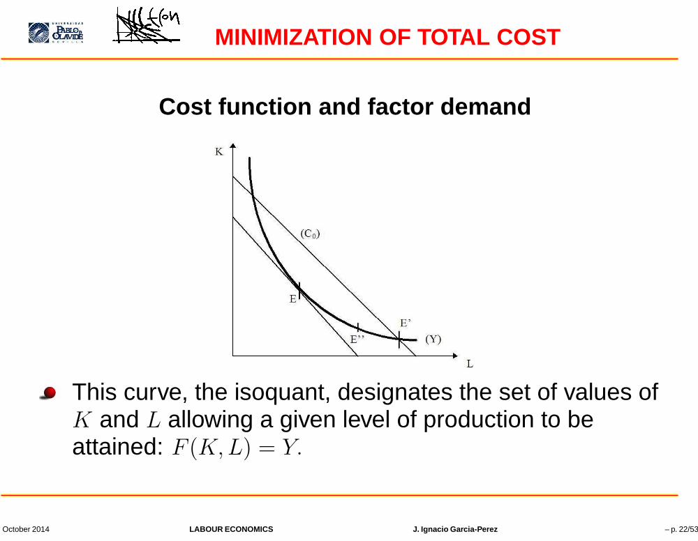
This curve, the isoquant, designates the set of values ofK and L allowing a given level of production to beattained: F (K,L) = Y.




The slope of this curve is negative, and the absolute value of its derivative is equal tothe technical rate of substitution between capital and labour, or |K′(L)| = FL/FK .

This technical rate of substitution defines the quantity of capital that can be savedwhen the quantity of labour is augmented by one unit.

In this figure we have also represented an iso-cost curve (C0).

This corresponds to the values of K and L such that WL+RK = C0, where C0 is apositive given constant.

An iso-cost curve is thus a straight line with a slope −(W/R) moving out towards thenorth-west when C0 increases.

It is evident, then, that if the iso-cost line is not tangent to the isoquant (at E′), it isalways possible to find a combination of factors K and L satisfying the constraintF (K,L) ≥ Y and leading to a cost inferior to that of the combination represented bypoint E′.




For that, we need only cause line (C0) to move in towards the origin (for example, atpoint E′′ the total cost of production is inferior to its value at point E′).

To sum up, the producer’s optimum lies at point E where the iso-cost line is tangent tothe isoquant.

The property of strict convexity of the isoquant guarantees that point E represents aunique minimum for the cost of production.

At this point, the technical rate of substitution is equal to the ratio of the costs of inputs.The conditional demands for capital and labour are thus defined by:

FL(K, L)

FK(K, L)=

W

Rand F (K, L) = Y(8)



The properties of the cost function

Relation (8) shows that K and L depend only on Y and W/R.

Evidently we could deduce the properties of the conditional demands using the twoequations of relation (8).

In fact, it is simpler to proceed indirectly by relying on the properties of the costfunction:

1. It is increasing in its arguments and homogeneous of degree 1 in (W,R).

2. It is concave in (W,R),.

3. It satisfies Shephard’s lemma, or:

L = CW (W,R, Y ) and K = CR(W,R, Y )(9)

where CW and CR are the partial derivatives of the cost function.

4. It is homogeneous of degree 1/θ with respect to Y when the production functionis homogeneous of degree θ.


PROPERTIES OF CONDITIONAL DEMANDS

These properties of the cost function allow us to derivethe properties of the conditional factor demands veryeasily

The most important properties of the conditionaldemands for labour and capital have to do with the waythey vary in the wake of a rise or a fall in the prices ofthese factors.

The extent of these variations depends on:

1. the elasticity of substitution between capital andlabour

2. the share of each factor in the total cost.



Variations in factor prices

The differentiation of the first relation of Shephard’s lemma (9) with respect to W

entails:∂L

∂W= CWW ≤ 0(10)

The conditional labour demand is thus decreasing with the price of this factor.

Since the first-order conditions (8) show that conditional demand in reality dependsonly on the relative price of labour, i.e. on W/R, we can state that it increases with theprice of capital.

Symmetrically, we could show that the conditional demand for capital diminishes withR and increases with W.

Shephard’s lemma allows us to characterize more precisely the cross effects of achange in the price of a factor on the demand for the other factor.



Variations in factor prices

Thus relation (9) immediately entails:

∂L

∂R=

∂K

∂W= CWR(11)

Since it was shown above that the conditional demand for a factor is increasing withthe price of the other factor, we can deduce that the cross derivative CWR isnecessarily positive.

The equality (11) portrays the symmetry condition of cross-price effects.

It means that at the producer’s optimum, the effect of a rise of one dollar in the price oflabour on the volume of capital is equal to the effect of a rise of one dollar in the priceof capital on the volume of labour.

This (astonishing) equality is no longer verified in terms of elasticities.



Cross elasticities and the elasticity of substitution

Let us recall first that the cross elasticities ηLR and ηKW of the conditional demand for afactor with respect to the price of the other factor are defined by:

ηLR =R

L

∂L

∂Rand ηKW =

W

K

∂K

∂W(12)

At the producer’s optimum, relation (11) then entails ηLR = (RK/WL)ηKW .

Consequently, leaving aside the exceptional case where the cost WL of manpowerwould equal the cost RK of capital, the cross elasticities will always be different.

They do not, therefore, constitute a significant indicator of the possibilities ofsubstitution between these two factors.




To get round this problem, it is preferable to resort to the notion of elasticity ofsubstitution which is the elasticity of the variable K/L with respect to relative priceW/R.

The elasticity of substitution between capital and labour, denoted by σ, is defined by:

σ =W/R

K/L

∂(K/L)

∂(W/R)(13)

This formula indicates that the capital-labour ratio increases by σ% when the ratiobetween the price of labour and the price of capital increases by 1%.

The figure with the isoqant shows that a rise (or a fall) of the relative price W/R

increases (or diminishes) the slope of the straight lines of iso-cost and therefore shiftspoint E towards the left (or the right) along the isoquant.




In other words, the ratio K/L varies in the same direction as the relative price W/R.

The elasticity of substitution between capital and labour is thus always positive.

When the value of the elasticity of substitution is high, that means that to obtain agiven level of production, the entrepreneur has the possibility of diminishing “greatly”the utilization of one factor and “greatly” increasing that of the other, in the wake of achange in the relative price of the factors.

Thus, when W rises or R falls, the firm’s interest in diminishing the utilization of labour

so as to minimize the total cost is all the greater, the higher the value of σ is. That

explains why the elasticities of conditional labour demand are increasing, in absolute

value, with the elasticity of substitution σ.



Variation in the level of output

The effects of an exogenous change in the level of output Y on the total cost are easilycharacterized if total cost is defined by C = WL+RK with F (K, L) = Y.

It suffices to differentiate these last two equalities with respect to Y and to take accountof the optimality condition (8) to get the following expression of the marginal cost :

CY (W,R, Y ) =W

FL

=R

FK

(14)

In the first place, it is apparent that the marginal cost is always positive.

That the total cost rises with the level of output.

Conversely, it is not possible to know the direction of variations in factor demandswithout supplementary hypotheses.

Clearly, factor demands do not diminish simultaneously when production increases.



Variation in the level of output

Thus a rise in production simply requires that the volume of one of the factors increase,but the volume of the other factor is not obliged to do so; it can even decrease.

However, when the production function satisfies the homogeneity hypothesis (6) amore precise conclusion emerges.

The factor demands are then homogeneous of degree 1/θ with respect to Y — seeproperty (iv) of the cost function set out in section 1.2.1 — and relation (??) clearlyshows that the conditional demands for labour and capital then rise simultaneouslywith the level of output.

Minimization of cost for a given level of output constitutes the first stage of the problem

of the firm; we must now examine how the optimal volume of output is determined.



SCALE EFFECTS

The entrepreneur is generally in a position to choose his or her level of production.

The desired quantities of the factors are then distinguishable from their conditionaldemands.

The analysis of substitution and scale effects yields highly general properties for labourdemand;

among other things, it brings into play the elasticity of substitution between capital andlabour, the share of each factor in the total cost, and the market power of the firm.

Let us again designate by P (Y ) the inverse demand function.

Then, profit Π(W,R, Y ) linked to a level of production Y when the unit costs of labourand capital are respectively W and R, takes the following form:

Π(W,R, Y ) = P (Y )Y − C(W,R, Y )(15)



SCALE EFFECTS

The first-order condition is obtained by setting the derivative of this expression to zero.

Rearranging terms, we find that the optimal level of production is characterized by:

P (Y ) = νCY (W,R, Y ) with ν ≡ 1/(1 + ηPY )(16)

We can see that the firm sets its price by applying the markup ν to its marginal costCY .

Taking into account expression (14) of marginal cost, the optimality condition (16)takes the following form:

FL(K,L) = νW

Pand FK(K,L) = ν

R

P(17)

In other words, at the firm’s optimum the marginal productivity of each factor is equal toits real cost multiplied by the markup.


UNCONDITIONAL FACTOR DEMANDS

When the competition in the market for the goodproduced by the firm is perfect (ν = 1), we rediscoverthe usual equalities between the marginal productivityof a factor and its real cost.

The values of K and of L, defined by equations (16)and (17), are called the long-run or unconditionaldemands for capital and for labour

We will study now THE LAWS OF DEMAND which referto the manner in which unconditional demands for thefactors of production vary with the unit costs of thesesame factors.

They combine substitution and scale effects.



Decreasing relation between the factor demand and its cost

We will see that the unconditional demand for a factor is decreasing with its cost.

This property possesses a very general character: in particular, it does not depend onthe production function of the firm being homogeneous.

To demonstrate this result, we have to use the profit function, denoted by Π(W,R),

equal to the maximal value of profit for given values of the costs of the inputs.

The cost function C(W,R, Y ) being concave in (W,R) for all Y, relation (15) signifiesthat function Π(W,R, Y ) is convex in (W,R) whatever the value of Y may be.

Moreover, Shephard’s lemma (9) states that the partial derivative CW (W,R, Y ∗) isequal to unconditional labour demand L∗.

An analogous rationale evidently applies to the unconditional capital demand K∗.

We thus arrive at the following relations, known as Hotelling’s lemma:

ΠW (W,R) = −L∗ and ΠR(W,R) = −K∗(18)



LABOUR DEMAND ELASTICITIES

It is possible to be more exact about unconditional labour demand L∗ by noting that italways satisfies Shephard’s lemma (9).

Thus we have L∗ = CW (W,R, Y ∗).

Differentiating this equality with respect to W, we get: ∂L∗

∂W= CWW + CWY

∂Y ∗

∂W

When we multiply the two members of this relation by W/L∗, we bring to light theelasticities ηLW and ηYW of unconditional labour demand and of the level of output withrespect to the wage.

The result is:

ηLW =W

L∗CWW +

(

Y ∗CWY

L∗

)

ηYW(19)

Since L∗ = CW (W,R, Y ∗), the terms (W/L∗)CWW and (Y ∗/L∗)CWY designaterespectively the elasticty ηLW of the conditional labour demand and the elasticity of thisdemand with respect to the level of output taken at point Y = Y ∗, ηLY .




We thus finally obtain:

ηLW = ηLW + ηLY ηYW(20)

This relation reveals the different effects of a rise in wage on the demand for labour:

We may start by isolating a substitution effect represented by the elasticity ηLW ofconditional labour demand.

We have seen before that this term is always negative, since for a given level ofproduction, a rise in the cost of labour always leads to reduced utilization of thisfactor (and increased utilization of capital).

Relation (20) likewise brings out a scale effect represented by the product ηLY ηYW .

The direction of this scale effect is obtained by noting that the second-orderconditions of the firm’s profit maximization dictate that ηYW should be of opposedsign to CWY .

Following Shephard’s lemma (9), ηLY is of the same sign as CWY , so the scaleeffect is always negative and therefore accentuates the substitution effect.




Using the same procedure, it is possible to calculate the cross elasticity ηLR of theunconditional labour demand with respect to the cost of capital. This comes to:

ηLR = ηLR + ηLY ηYR(21)

In the case of two inputs, we have shown that the conditional demand for a factor riseswhen the price of the other factor rises.

The substitution effect, the term ηLR, is thus positive.

Conversely, the scale effect, represented by the term ηLY ηYR,, is a priori ambiguous.

The sign of cross elasticity ηLR is thus undetermined.

If ηLR > 0, labour and capital are qualified as gross substitutes: a rise in the priceof capital causes demand for this factor to fall and that of labour to rise.

If ηLR < 0, labour and capital are qualified as gross complements: a hike in theprice of one of these factors signifies that demand for both of them falls of.


DYNAMIC LABOUR DEMAND

The static theory of labour demand furnishes valuable indications about whatdetermines elasticities, and about the possibilities of substitution over the long runbetween the different inputs.

But it gives no detail about the manner in which the inputs reach their long-run valuesor about the length of time that these adjustments take.

Moreover, it does not take into account the fact that firms are faced with an ongoingprocess of reorganization arising from technological constraints, market fluctuations,and manpower mobility.

In order to be able to assess these phenomena, we have to resort to the notion ofadjustment cost.

Firms may incur adjustment costs when they decide to change their level ofemployment.

But the fact that firms must deal with quits by workers entails that they may incuradjustment costs simply in order to maintain a constant level of employment.



No real consensus has yet been reached as regards the analytical representation ofthese costs, but the quadratic symmetric form, historically the one most frequentlyutilized, is today gradually being abandoned.

We will examine the dynamics of labour demand in a setting without uncertainty,although there exist important stochastic elements in these problems.

labour adjustment costs arise from variations in the volume of employment, and fromthe replacement of former employees by new ones.

Numerous studies show that the size of these costs is far from insignificant, and forthat reason they play a large role in decisions to hire and fire.

In France, the average cost of a separation represents 56% of the annual cost oflabour, whereas a hire represents only 3.3%.

Most assessments conclude that employment protection is less strict in the US,Canada, and the UK than in continental Europe.

In Europe, a large part of the cost of termination is regulatory in nature (period ofadvance notice, administrative procedure, etc.). The result has been a massiverecourse to short-term contracts.



For ease of analysis, adjustment costs have most often been represented using aconvex symmetric function (in general quadratic) of net employment changes.

But this way of specifying them does not allow us to explain asymmetric anddiscontinuous adjustments in employment and the consequence of gross employmentchanges.

For this reason, it is now gradually being replaced by a representation including fixedcosts, linear costs, quadratic costs and gross employment changes.

Quadratic costs

This representation was introduced by Holt et al. (1960), who viewed net adjustmentcosts as equal to b(∆Lt − a)2, a, b > 0, with ∆Lt = Lt − Lt−1 or ∆Lt = Lt

according to whether time was represented discretely or continuously.

This specification has the advantage of introducing an asymmetry between the cost of

positive and negative variations in employment (a > 0).



Linear costs

The specification of adjustment costs in the form of a piecewise linear function offersthe advantage of achieving a more realistic representation of labour demand,

in which firms hire in some circumstances, let employees go in others, and sometimesleave their workforce unchanged

The utilization of piecewise linear costs has greatly expanded in the 1990s, with theworks of Bentolila and Bertola (1990), who examine linear adjustment costs of theform:

C(∆L) = ch∆L if ∆L ≥ 0 and C(∆L) = −cf∆L if ∆L ≤ 0, ch > 0, cl > 0

(22)

The coefficients ch and cf represent the respective unit costs of a hiring and a

termination. The adjustment of employment is asymmetric, since ch 6= cf .



Quadratic and symmetric adjustment costs

We here consider a firm situated in a deterministic environment, which must supportadjustment costs when it alters its workforce.

To make things easier from a technical point of view, a large part of the literature hasassumed that these costs were symmetric and could be represented by a quadraticfunction.

We shall work with a dynamic model in continuous time, in which, at each date, t ≥ 0,

the adjustment cost is restricted to labour alone.

When the firm utilizes a quantity Lt of this factor, it obtains a level of output F (Lt) thatis strictly increasing and concave with respect to Lt.

Taking other inputs into account, like capital for example, greatly complicates theanalysis without changing the import of the results which we want to highlight.

We likewise simplify by leaving quits out of the reckoning, on the assumption that netvariations in employment are equal to gross variations.




Let Lt be the derivative with respect to t of the variable Lt;

we shall assume that variations in the level of employment are accompanied at everydate t by an adjustment cost represented by the quadratic function (b/2)Lt

2, b ≥ 0.

To simplify the notations and calculations, from now on we will omit the index t andassume that at every date the cost of labour and the interest rate are exogeneousconstants denoted respectively by W and r.

At date t = 0, the discounted present value of profit, Π0, is written:

Π0 =

∫

+∞

0

[

F (L)−WL−b

2L2

]

e−rtdt(23)

In this environment, free of random factors, the firm chooses its present and futurelevels of employment so as to maximize the discounted present value of profits Π0.




This is a classic problem of calculus of variations for which the first-order condition isgiven by the Euler equation

After several simple calculations, we find that the employment path is described by anon-linear second-order differential equation that takes the form:

bL− rbL+ F ′(L)−W = 0(24)

The stationary value L∗ of employment is obtained by making L = L = 0 in thisequation.

Given the difficulty of this model, we will skip the analysis of the dynamics ofemployment in this case so we will continue by studying the case of linear adjustmentcosts.



Linear and asymmetric adjustment costs

It is possible to distinguish the costs of hiring and firing by adopting a piecewise linearspecification.

The hypothesis of linearity also brings out the fact that, contrary to the model withquadratic costs, employment adjustment can take place immediately.

Let ch and cf be two positive constants, and let us assume from now on that theadjustment costs are represented by the function:

C(L) = cL with c = ch if L > 0 and c = −cf if L < 0(25)

Parameters ch and cf allow us to distinguish hiring costs (L > 0) from terminationcosts (L < 0).

As in the previous model with quadratic adjustment costs, it is assumed, for the sake ofsimplicity, that there are no quits.




The problem of the firm consists of choosing, at date t = 0, levels of employment thatmaximize the discounted present value of profit Π0. The latter is expressed thus:

Π0 =

∫

+∞

0

[

F (L)−WL− C(L)]

e−rtdt(26)

Once again, this is a problem of calculus of variations to which the Euler equation (??)applies when the quadratic function −(b/2)L2 is replaced by the linear functionC(L) = cL.

After several simple calculations, we find that the employment path is defined by theequation F ′(L) = W + rc, which entails:

F ′(L) = W + rch if L > 0, and F ′(L) = W − rcf if L < 0(27)




These conditions signify that the firm hires when marginal productivity is sufficientlyhigh to cover the wage W and the hiring cost rch.

Conversely, the firm fires when productivity is so low that it just equals wage W lessthe provision rcf for the termination cost.

In all other cases, i.e. when productivity lies in the interval [W − rcf , W + rch], thefirm has no interest in altering the size of its workforce, for the gains due to hiring andfiring are less than the costs incurred by adjusting employment.

labour adjustments take a particularly instructive form when the parameters W, r, chand cf are constants, which we have assumed.

Let us define the employment levels Lh and Lf , by the equalities:

F ′(Lh) = W + rch and F ′(Lf ) = W − rcf(28)




In this case, the optimal values Lh and Lf do not depend on date t.

That means that labour demand immediately (i.e. in t = 0) “jumps” to its stationaryvalue.

The firm adjusts its workforce to the value Lh (or Lf ) if the latter is superior (orinferior) to the initial value L0 of employment.

In the opposite case, i.e. if L0 falls in the interval [Lh, Lf ], the optimal solution for thefirm consists of making no change to the size of its workforce.

In sum, labour demand is defined by:

L =

Lh if L0 ≤ Lh

L0 if Lh ≤ L0 ≤ Lf

Lf if Lf ≤ L0

(29)




Relations (28) show us that the costs of hiring and firing have opposing effects onlabour demand.

If the size of the workforce is low at the outset (L0 ≤ Lh), then optimal employment isequal to Lh and a rise in the hiring cost ch reduces employment.

Conversely, if there is a large number of workers at the outset (Lf ≤ L0), the optimallevel of employment takes the value Lf and we clearly see that a rise in thetermination cost cf has the effect of increasing employment.

We should not, however, conclude on the basis of this analysis that a rise in thetermination cost (or a fall in the hiring cost) “augments” the firm’s labour demand.

In reality, since this demand immediately jumps to Lh or Lf (unless it simply remainsat L0), the level of employment is always equal to one of the three quantities Lh, Lf

or L0.




Let us suppose that the number of workers is Lf , a rise in the termination cost cf willaugment Lf up to a certain value L+

f, and will thus have the effect of placing the

outset level of the workforce (now equal to Lf ) somewhere in the interval [Lh, L+

f].

In this case, relation (29) describing labour demand shows that the firm then has aninterest in remaining at Lf .

In other words, a rise in the cost of terminating hinders the firm from going ahead withreductions in personnel, but gives it no incentive to hire.

An analogous line of reasoning would show that a rise in the costs of hiring has theeffect of discouraging further recruitment, but does not lead to a reduction inemployment.

Conversely, a reduction in hiring costs always has a positive effect on employment tothe extent that it increases the value Lh of optimal employment.


Chapter 2: LABOUR DEMANDINTRODUCTION An entrepreneur has an interest in hiring a worker whenever the...

Documents

Transcript of Chapter 2: LABOUR DEMANDINTRODUCTION An entrepreneur has an interest in hiring a worker whenever the...