Chapter 2 Fundamentals of ANSYS - buecher.de · E. Madenci, I. Guven, The Finite Element Method and...

15

Chapter 2Fundamentals of ANSYS

© Springer International Publishing 2015 E. Madenci, I. Guven, The Finite Element Method and Applications in Engineering Using ANSYS ®, DOI 10.1007/978-1-4899-7550-8_2

2.1 Useful Definitions

Before delving into the details of the procedures related to the ANSYS program, we define the following terms:

Jobname A specific name to be used for the files created during an ANSYS ses-sion. This name can be assigned either before or after starting the ANSYS program.

Working Directory A specific folder (directory) for ANSYS to store all of the files created during a session. It is possible to specify the Working Directory before or after starting ANSYS.

Interactive Mode This is the most common mode of interaction between the user and the ANSYS program. It involves activation of a platform called Graphical User Interface ( GUI), which is composed of menus, dialog boxes, push-buttons, and dif-ferent windows. Interactive Mode is the recommended mode for beginner ANSYS users as it provides an excellent platform for learning. It is also highly effective for postprocessing.

Batch Mode This is a method to use the ANSYS program without activating the GUI. It involves an Input File written in ANSYS Parametric Design Language ( APDL), which allows the use of parameters and common programming features such as DO loops and IF statements. These capabilities make the Batch Mode a very powerful analysis tool. Another distinct advantage of the Batch Mode is realized when there is an error/mistake in the model generation. This type of problem can be fixed by modifying a small portion of the Input File and reading it again, saving the user a great deal of time.

Combined Mode This is a combination of the Interactive and Batch Modes in which the user activates the GUI and reads the Input File. Typically, this method allows the user to generate the model and obtain the solution using the Input File while reviewing the results using the Postprocessor within the GUI. This method combines the salient advantages of the Interactive and Batch Modes.

16 2 Fundamentals of ANSYS

2.2 Before an ANSYS Session

The construction of solutions to engineering problems using FEA requires either the development of a computer program based on the FEA formulation or the use of a commercially available general-purpose FEA program such as ANSYS. The ANSYS program is a powerful, multi-purpose analysis tool that can be used in a wide variety of engineering disciplines. Before using ANSYS to generate an FEA model of a physical system, the following questions should be answered based on engineering judgment and observations:

• What are the objectives of this analysis?• Should the entire physical system be modeled, or just a portion?• How much detail should be included in the model?• How refined should the finite element mesh be?

In answering such questions, the computational expense should be balanced against the accuracy of the results. Therefore, the ANSYS finite element program can be employed in a correct and efficient way after considering the following:

• Type of problem.• Time dependence.• Nonlinearity.• Modeling idealizations/simplifications.

Each of these topics is discussed in this section.

2.2.1 Analysis Discipline

The ANSYS program is capable of simulating problems in a wide range of engi-neering disciplines. However, this book focuses on the following disciplines:

Structural Analysis Deformation, stress, and strain fields, as well as reaction forces in a solid body.

Thermal Analysis Steady-state or time-dependent temperature field and heat flux in a solid body.

2.2.1.1 Structural Analysis

This analysis type addresses several different structural problems, for example:

Static Analysis The applied loads and support conditions of the solid body do not change with time. Nonlinear material and geometrical properties such as plasticity, contact, creep, etc., are available.

Modal Analysis This option concerns natural frequencies and modal shapes of a structure.


Harmonic Analysis The response of a structure subjected to loads only exhibiting sinusoidal behavior in time.

Transient Dynamic The response of a structure subjected to loads with arbitrary behavior in time.

Eigenvalue Buckling This option concerns the buckling loads and buckling modes of a structure.

2.2.1.2 Thermal Analysis

This analysis type addresses several different thermal problems, for example:

Primary Heat Transfer Steady-state or transient conduction, convection and radiation.

Phase Change Melting or freezing.

Thermomechanical Analysis Thermal analysis results are employed to compute displacement, stress, and strain fields due to differential thermal expansion.

2.2.1.3 Degrees of Freedom

The ANSYS solution for each of these analysis disciplines provides nodal values of the field variable. This primary unknown is called a degree of freedom (DOF). The degrees of freedom for these disciplines are presented in Table 2.1. The analysis discipline should be chosen based on the quantities of interest.

2.2.2 Time Dependence

The analysis with ANSYS should be time-dependent if:

• The solid body is subjected to time varying loads.• The solid body has an initially specified temperature distribution.• The body changes phase.

Table 2.1 Degrees of freedom for structural and thermal analysis disciplines

Discipline Quantity DOFStructural Displacement, stress, strain, reaction forces DisplacementThermal Temperature, flux Temperature


2.2.3 Nonlinearity

Most real-world physical phenomena exhibit nonlinear behavior. There are many situations in which assuming a linear behavior for the physical system might pro-vide satisfactory results. On the other hand, there are circumstances or phenomena that might require a nonlinear solution. A nonlinear structural behavior may arise because of geometric and material nonlinearities, as well as a change in the bound-ary conditions and structural integrity. These nonlinearities are discussed briefly in the following subsections.

2.2.3.1 Geometric Nonlinearity

There are two main types of geometric nonlinearity:

Large Deflection and Rotation If the structure undergoes large displacements compared to its smallest dimension and rotations to such an extent that its original dimensions and position, as well as the loading direction, change significantly, the large deflection and rotation analysis becomes necessary. For example, a fishing rod with a low lateral stiffness under a lateral load experiences large deflections and rotations.

Stress Stiffening When the stress in one direction affects the stiffness in another direction, stress stiffening occurs. Typically, a structure that has little or no stiffness in compression while having considerable stiffness in tension exhibits this behavior. Cables, membranes, or spinning structures exhibit stress stiffening.

2.2.3.2 Material Nonlinearity

A typical nonlinear stress-strain curve is given in Fig. 2.1. A linear material re-sponse is a good approximation if the material exhibits a nearly linear stress-strain

Fig. 2.1 Non-linear material response


curve up to a proportional limit and the loading is in a manner that does not create stresses higher than the yield stress anywhere in the body.

Nonlinear material behavior in ANSYS is characterized as:

Plasticity Permanent, time-independent deformation.

Creep Permanent, time-dependent deformation.

Nonlinear Elastic Nonlinear stress-strain curve; upon unloading, the structure returns back to its original state—no permanent deformations.

Viscoelasticity Time-dependent deformation under constant load. Full recovery upon unloading.

Hyperelasticity Rubber-like materials.

2.2.3.3 Changing-status Nonlinearity

Many common structural features exhibit nonlinear behavior that is status depen-dent. When the status of the physical system changes, its stiffness shifts abruptly. The ANSYS program offers solutions to such phenomena through the use of nonlin-ear contact elements and birth and death options. This type of behavior is common in modeling manufacturing processes such as that of a shrink-fit (Fig. 2.2).

2.2.4 Practical Modeling Considerations

In order to reduce computational time, minor details that do not influence the results should not be included in the FE model. Minor details can also be ignored in order to render the geometry symmetric, which leads to a reduced FE model. However, in certain structures, “small” details such as fillets or holes may be the areas of

Fig. 2.2 Element birth and death used in a manufacturing problem


maximum stress, which might prove to be extremely important in the analysis and design. Engineering judgment is essential to balance the possible gain in computa-tional cost against the loss of accuracy.

2.2.4.1 Symmetry Conditions

If the physical system under consideration exhibits symmetry in geometry, material properties, and loading, then it is computationally advantageous to model only a representative portion. If the symmetry observations are to be included in the model generation, the physical system must exhibit symmetry in all of the following:

• Geometry.• Material properties.• Loading.• Degree of freedom constraints.

Different types of symmetry are:

• Axisymmetry.• Rotational symmetry.• Planar or reflective symmetry.• Repetitive or translational symmetry.

Examples for each of the symmetry types are shown in Fig. 2.3. Each of these sym-metry types is discussed below.

Axisymmetry As illustrated in Fig. 2.4, axisymmetry is the symmetry about a cen-tral axis, as exhibited by structures such as light bulbs, straight pipes, cones, circular plates, and domes.

Fig. 2.4 Different views of a 3-D body with axisymmetry and its cross section (far right)

Fig. 2.3 Types of symmetry conditions (from left to right): axisymmetry, rotational, reflective/planar, and repetitive/translational


Rotational Symmetry A structure possesses rotational symmetry when it is made up of repeated segments arranged about a central axis. An example is a turbine rotor (see Fig. 2.5).

Planar or Reflective Symmetry When one-half of a structure is a mirror image of the other half, planar or reflective symmetry exists, as shown in Fig. 2.6. In this case, the plane of symmetry is located on the surface of the mirror.

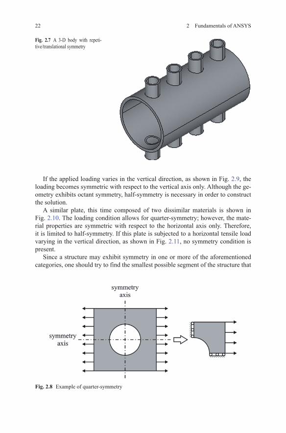
Repetitive or Translational Symmetry Repetitive or translational symmetry exists when a structure is made up of repeated segments lined up in a row, such as a long pipe with evenly spaced cooling fins, as shown in Fig. 2.7.

Symmetry in Material Properties, Loading, Displacements Once symmetry in geometry is observed, the same symmetry plane or axis should also be valid for the material properties, loading (forces, pressure, etc.), and constraints. For example, a homogeneous and isotropic square plate with a hole at the center under horizontal tensile loading (Fig. 2.8) has octant (1/8th) symmetry in both geometry and material with respect to horizontal, vertical, and both diagonal axes. However, the loading is symmetric with respect to horizontal and vertical axes only. Therefore, a quarter of the structure is required in the construction of the solution.

Fig. 2.6 Different views of a 3-D body with reflective/planar symmetry

Fig. 2.5 Different views of a 3-D body with rotational symmetry


If the applied loading varies in the vertical direction, as shown in Fig. 2.9, the loading becomes symmetric with respect to the vertical axis only. Although the ge-ometry exhibits octant symmetry, half-symmetry is necessary in order to construct the solution.

A similar plate, this time composed of two dissimilar materials is shown in Fig. 2.10. The loading condition allows for quarter-symmetry; however, the mate-rial properties are symmetric with respect to the horizontal axis only. Therefore, it is limited to half-symmetry. If this plate is subjected to a horizontal tensile load varying in the vertical direction, as shown in Fig. 2.11, no symmetry condition is present.

Since a structure may exhibit symmetry in one or more of the aforementioned categories, one should try to find the smallest possible segment of the structure that

Fig. 2.8 Example of quarter-symmetry

Fig. 2.7 A 3-D body with repeti-tive/translational symmetry


would represent the entire structure. If the physical system exhibits symmetry in geometry, material properties, loading, and displacement constraints, it is compu-tationally advantageous to use symmetry in the analysis. Typically, the use of sym-metry produces better results as it leads to a finer, more detailed model than would otherwise be possible.

A three-dimensional finite element mesh of the structure shown in Fig. 2.12 con-tains 18,739 tetrahedral elements with 5014 nodes. However, the two-dimensional mesh of the cross section necessary for the axisymmetric analysis has 372 quadrilat-eral elements and 447 nodes. The use of symmetry in this case reduces the CPU time required for the solution while delivering the same level of accuracy in the results.

Fig. 2.10 Example of half-symmetry with respect to horizontal axis

Fig. 2.9 Example of half-symmetry with respect to vertical axis

Fig. 2.11 Example of no symmetry


2.2.4.2 Mesh Density

In general, a large number of elements provide a better approximation of the solu-tion. However, in some cases, an excessive number of elements may increase the round-off error. Therefore, it is important that the mesh is adequately fine or coarse in the appropriate regions. How fine or coarse the mesh should be in such regions is another important question. Unfortunately, definitive answers to the questions about mesh refinement are not available since it is completely dependent on the specific physical system considered. However, there are some techniques that might be helpful in answering these questions:

Adaptive Meshing The generated mesh is required to meet acceptable energy error estimate criteria. The user provides the “acceptable” error level information. This type of meshing is available only for linear static structural analysis and steady-state thermal analysis.

Mesh Refinement Test Within ANSYS An analysis with an initial mesh is per-formed first and then reanalyzed by using twice as many elements. The two solutions are compared. If the results are close to each other, the initial mesh configuration is considered to be adequate. If there are substantial differences between the two, the analysis should continue with a more-refined mesh and a subsequent comparison until convergence is established.

Submodeling If the mesh refinement test yields nearly identical results for most regions and substantial differences in only a portion of the model, the built-in “sub-modeling” feature of ANSYS should be employed for localized mesh refinement. This feature is described in Chap. 11.

Fig. 2.12 Three-dimensional mesh of a structure ( left) and 2-D mesh of the same structure ( right) using axisymmetry

http://www.springer.com/978-1-4899-7549-2

Chapter 2 Fundamentals of ANSYS - buecher.de · E. Madenci, I. Guven, The Finite Element Method and...

Documents

Transcript of Chapter 2 Fundamentals of ANSYS - buecher.de · E. Madenci, I. Guven, The Finite Element Method and...