Chapter 14 Simultaneous Equations Models 14.1 …econ446/wiley/Chapter14.pdf · • Simultaneous...

Chapter 14

Simultaneous Equations Models

14.1 Introduction

• Simultaneous equations models differ from those we have considered in previous

chapters because in each model there are two or more dependent variables rather than

just one.

• Simultaneous equations models also differ from most of the econometric models we

have considered so far because they consist of a set of equations

• The least squares estimation procedure is not appropriate in these models and we must

develop new ways to obtain reliable estimates of economic parameters.

Slide 14.1

Undergraduate Econometrics, 2nd Edition-Chapter 14

14.2 A Supply and Demand Model

• Supply and demand jointly determine the market price of a good and the amount of it

that is sold

• An econometric model that explains market price and quantity should consist of two

equations, one for supply and one for demand.

1 2Demand: dq p y e= α + α + (14.2.1)

1Supply: sq p eβ + (14.2.2) =

• In this model the variables p and q are called endogenous variables because their

values are determined within the system we have created.

• The income variable y has a value that is given to us, and which is determined outside

this system. It is called an exogenous variable.

Slide 14.2


• Random errors are added to the supply and demand equations for the usual reasons,

and we assume that they have the usual properties

2

2

( ) 0, var( )

( ) 0, var( )cov( , ) 0

d d d

s s s

d s

E e e

E e ee e

= = σ

= σ=

(14.2.3) =

• The fact that p is random means that on the right-hand side of the supply and demand

equations we have an explanatory variable that is random.

• This is contrary to the assumption of “fixed explanatory variables” that we usually

make in regression model analysis.

• Furthermore p and the random errors, ed and es, are correlated, making the least squares

estimator biased and inconsistent.

Slide 14.3


14.3 The Reduced Form Equations

• The two structural equations (14.2.1) and (14.2.2) can be solved, to express the

endogenous variables p and q as functions of the exogenous variable y.

• This reformulation of the model is called the reduced form of the structural equation

system.

• To find the reduced form we solve (14.2.1) and (14.2.2) simultaneously for p and q.

• To solve for p, set q in the demand and supply equations to be equal,

1 1 2s dp e p y eβ + = α + α +

Slide 14.4


• Then solve for p,

( ) ( )2

1 1 1 1

1 1

d se ep y

y v

α −= +

β −α β −α

= π +

(14.3.1)

Substitute p into equation 14.2.2 and simplify.

( ) ( )

( ) ( )

21 1

1 1 1 1

1 2 1 1

1 1 1 1

2 2

d ss s

d s

e eq p e y e

e ey

y v

⎡ ⎤α −= β + = β + +⎢ ⎥β −α β −α⎣ ⎦

β α β −α= +

β −α β −α

= π +

(14.3.2)

Slide 14.5


• The parameters π1 and π2 in equations 14.3.1 and 14.3.2 are called reduced form

parameters.

• The error terms and are called reduced form errors, or disturbance terms. 1v 2v

• The reduced form equations can be estimated consistently by least squares.

• The least squares estimator is BLUE for the purposes of estimating π1 and π2.

• The reduced form equations are important for economic analysis.

• These equations relate the equilibrium values of the endogenous variables to the

exogenous variables. Thus, if there is an increase in income y, 1π is the expected

increase in price, after market adjustments lead to a new equilibrium for p and q.

• Secondly the estimated reduced form equations can be used to predict values of

equilibrium price and quantity for different levels of income.

Slide 14.6


14.4 The Failure of Least Squares Estimation in Simultaneous Equations Models

1 2Demand: dq p y e= α + α + (14.2.1)

1Supply: sq p eβ + (14.2.2) =

• In the supply equation, (14.2.2), the random explanatory variable p on the right-hand

side of the equation is correlated with the error term es.

Slide 14.7


14.4.1 An Intuitive Explanation of the Failure of Least Squares

• Suppose there is a small change, or blip, in the error term es, say Δes.

• The blip Δes in the error term of (14.2.2) is directly transmitted to the equilibrium value

of p.

• This is clear from the reduced form equation 14.3.1. Every time there is a change in the

supply equation error term, es, it has a direct linear effect upon p.

• Since and , if Δe1 0β > 1 0α < s > 0, then 0pΔ < .

• Thus, every time there is a change in es there is an associated change in p in the

opposite direction. Consequently, p and es are negatively correlated.

Slide 14.8


• Ordinary least squares estimation of the relation between q and p gives “credit” to

price for the effect of changes in the disturbances.

• In large samples, the least squares estimator will tend to be negatively biased.

• This bias persists even when the sample size is large, and thus the least squares

estimator is inconsistent.

The least squares estimator of parameters in a structural simultaneous equation

is biased and inconsistent because of the correlation between the random error

and the endogenous variables on the right-hand side of the equation.

Slide 14.9


14.4.2 An Algebraic Explanation of the Failure of Least Squares

• First, let us obtain the covariance between p and es.

( ) ( ) ( )( ) ( )[ ]

( )

1 1

11 1

2

1 1

cov ,

[since 0]

[substitute for ]

[since is exogenous]

[since , assumed uncorrelated]

s s s

s s

s

d ss

sd s

p e E p E p e E e

E pe E e

E y v e p

e eE e y

E ee e

= − −⎡ ⎤ ⎡ ⎤⎣ ⎦ ⎣ ⎦= =

= π +

⎡ ⎤−= π⎢ ⎥β −α⎣ ⎦

−=β −α

=2

1 1

0s−σ<

β −α

(14.4.1)

Slide 14.10


• The least squares estimator in equation 14.2.2 is

1 2t t

t

p qb

p= ∑∑

(14.4.2)

• Substitute for q from equation 14.3.2 and simplify,

( )11 1 12 2

t t st tst

t t

p p e pb e h ep p

⎛ ⎞β += = β + = β⎜ ⎟⎜ ⎟

⎝ ⎠t st+∑ ∑ ∑∑ ∑

(14.4.3)

where

2t

tt

php

=∑

Slide 14.11


• The expected value of the least squares estimator is

( ) ( )1 1 1t stE b E h e= β + ≠ β∑ (14.4.4)

• The expectation ( ) 0t stE h e ≠ because es and p are correlated.

• In large samples there is a similar failure.

• Multiply through the supply equation by price, p, take expectations and solve.

( ) ( ) ( )

( )( )

( )( )

21

21

1 2 2

s

s

s

pq p pe

E pq E p E pe

E pq E peE p E p

= β +

= β +

β = −

(14.4.5)

Slide 14.12


• In large samples, as T→∞, sample analogs of expectations, which are averages,

converge to the expectations. That is, ( ) ( )2 2/ , /t t tq p T E pq p T E p→ →∑ ∑ .

• Consequently, because the covariance between p and es is negative, from equation

14.4.1,

( )( )

( )( )

( )( )

21 1

1 1 1 12 2 2 2

//

t t s s

t

q p T E pq E peb

p T E p E p E pσ β −α

= → =β + = β − < β∑∑

(14.4.6)

The least squares estimator of the slope of the supply equation, in large samples,

converges to a value less than β1.

Slide 14.13


14.5 The Identification Problem

• In the supply and demand model given by equations 14.2.1 and 14.2.2, the parameters

of the demand equation, α1 and α2, can not be consistently estimated by any estimation

method.

• The slope of the supply equation, β1, can be consistently estimated.

• The problem lies with the model that we are using. There is no variable in the supply

equation that will shift it relative to the demand curve.

• It is the absence of variables from an equation that makes it possible to estimate its

parameters. A general rule, which is called a condition for identification of an

equation, is this:

Slide 14.14


A Necessary Condition for Identification: In a system of M simultaneous

equations, which jointly determine the values of M endogenous variables, at

least M−1 variables must be absent from an equation for estimation of its

parameters to be possible. When estimation of an equation’s parameters is

possible, then the equation is said to be identified, and its parameters can be

estimated consistently. If less than M−1 variables are omitted from an equation,

then it is said to be unidentified and its parameters can not be consistently

estimated.

Slide 14.15


• In our supply and demand model there are M=2 equations and there are a total of three

variables: p, q and y.

• In the demand equation none of the variables are omitted; thus it is unidentified and its

parameters can not be estimated consistently.

• In the supply equation M−1=1 and one variable, income, is omitted; the supply curve

is identified and its parameter can be estimated.

• The identification condition must be checked before trying to estimate an equation.

Slide 14.16


Remark: The two-stage least squares estimation procedure is developed in

Chapter 13 and shown to be an instrumental variables estimator. The number

of instrumental variables required for estimation of an equation within a

simultaneous equations model is equal to the number of right-hand-side

endogenous variables. In a typical equation within a simultaneous equations

model several exogenous variables appear on the right-hand-side. Thus

instruments must come from those exogenous variables omitted from the

equation in question. Consequently, identification requires that the number of

omitted exogenous variables in an equation be at least as large as the number of

right-hand-side endogenous variables. This ensures an adequate number of

instrumental variables.

Slide 14.17


14.6 The Two-Stage Least Squares Estimation Procedure

• In this section we briefly describe two-stage least squares (2SLS) estimation

1 sq p e= β +

( )

(14.2.2)

• The variable p is composed of a systematic part, which is its expected value E(p), and a

random part, which is the reduced form random error v1.

1 1 1p E p v y v+ = π + (14.6.1) =

• In the supply equation (14.2.2) the portion of p that causes problems for the least

squares estimator is v1, the random part.

• Suppose we knew the value of π1. Then we could replace p in (14.2.2) by (14.6.1) to

obtain

Slide 14.18


1 1

1 1 1

1 *

[ ( ) ]( ) ( )( )

s

s

q E p v eE p v eE p e

= β + += β + β += β +

(14.6.2)

• We could apply least squares to equation 14.6.2 to consistently estimate β1.

• We can estimate π1 using 1π̂ from the reduced form equation for p.

• A consistent estimator for E(p) is

1垐p y= π

• Using as a replacement for E(p) in (14.6.2) we obtain p̂

1 *e垐q pβ + (14.6.3) =

Slide 14.19


• In large samples, and the random error are uncorrelated, and consequently the

parameter β

ˆ p *̂e

1 can be consistently estimated by applying least squares to (14.6.3).

• Estimating the equation 14.6.3 by least squares generates the so-called two-stage least

squares estimator of , which is consistent and asymptotically normal. 1β

Slide 14.20


13.4 An Example of Two Stage Least Squares Estimation

• Consider a supply and demand model for truffles:

demand: t ti e1 2 3 4d

t t tq p ps dα + α + α + α + (13.4.1) =

supply: 1 2 3s

t t t teq p pfβ + β + β + (13.4.2) =

• In the demand equation q is the quantity of truffles traded in a particular French market

at time t, p is the market price of truffles, ps is the market price of a substitute for real

truffles (another fungus much less highly prized), and di is per capita disposable

income.

Slide 14.21


• The supply equation contains the market price and quantity supplied. Also it includes

pf, the price of a factor of production, which in this case is the hourly rental price of

truffle-pigs used in the search process.

• In this model we assume that p and q are endogenous variables.

• The exogenous variables are ps, di, pf and the intercept variable.

Slide 14.22


13.4.1 Identification

• The rule for identifying an equation is that in a system of M equations at least M−1

variables must be omitted from each equation in order for it to be identified.

• In the demand equation the variable pf is not included and thus the necessary M−1=1

variable is omitted.

• In the supply equation both ps and di are absent; more than enough to satisfy the

identification condition.

• We conclude that each equation in this system is identified and can thus be estimated

by two-stage least squares.

Slide 14.23


13.4.2 The Reduced Form Equations

• The reduced form equations express each endogenous variable, p and q, in terms of the

exogenous variables ps, di, pf and the intercept variable, plus an error term.

11 21 31 41 1

12 22 32 42 2

t t t t t

t t t t t

q ps di pf v

p ps di pf v

= π + π + π + π +

= π + π + π + π +

• Data for each of the endogenous and exogenous variables are given in Table 13.1.

• The price p is measured in $ per ounce, q is measured in ounces, ps is measured in $

per pound, di is in $1000 and pf is the hourly rental rate for a truffle-finding pig.

Slide 14.24


Table 13.1 Sample Truffle Supply and Demand Data OBS p q ps di pf

1 9.88 19.89 19.97 21.03 10.52 2 13.41 13.04 18.04 20.43 19.6727 27.90 20.81 28.98 46.32 27.8028 27.00 14.95 18.52 48.94 30.3429 29.48 26.27 28.16 51.25 24.1230 35.15 20.65 28.43 48.36 34.01

Table 13.2a Reduced Form Equation for Quantity of Truffles (q) Variable Estimate Std. Error t-value p-valueConst 7.895 3.019 2.615 0.0147PS 0.656 0.133 4.947 0.0001DI 0.217 0.065 3.323 0.0026PF −0.507 0.113 −4.491 0.0001 Table 13.2b Reduced Form Equation for Price of Truffles (p) Variable Estimate Std. Error t-value p-valueConst −10.837 2.478 −4.374 0.0002PS 0.569 0.109 5.229 0.0001DI 0.253 0.054 4.736 0.0001PF 0.451 0.093 4.872 0.0001

Slide 14.25


• The reduced form equations are used to obtain ˆ tp which will be used in place of pt on

the right-hand side of the supply and demand equations in the second stage of two-

stage least squares.

12 22 32 42垐垐 ?10.837 .569 .253 .451

t t t t

t t t

p ps di pfps di pf

= π + π + π + π= − + + +

Slide 14.26


• The 2SLS results are given in Tables 13.3a and 13.3b.

Table 13.3a 2SLS Estimates for Truffle Demand (qd)

Variable Estimate Std. Error t-value p-value

Const −4.279 5.161 −0.829 0.4145

P −1.123 0.460 −2.441 0.0217

PS 1.296 0.331 3.919 0.0006

DI 0.501 0.213 2.359 0.0261

Table 13.3b 2SLS Estimates for Truffle Supply (qs)

Variable Estimate Std. Error t-value p-value

Const 20.033 1.160 17.264 0.0001

P 1.014 0.071 14.297 0.0001

PF −1.001 0.078 −12.784 0.0001

Slide 14.27


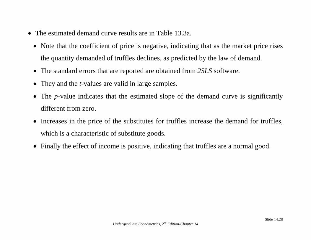
• The estimated demand curve results are in Table 13.3a.

• Note that the coefficient of price is negative, indicating that as the market price rises

the quantity demanded of truffles declines, as predicted by the law of demand.

• The standard errors that are reported are obtained from 2SLS software.

• They and the t-values are valid in large samples.

• The p-value indicates that the estimated slope of the demand curve is significantly

different from zero.

• Increases in the price of the substitutes for truffles increase the demand for truffles,

which is a characteristic of substitute goods.

• Finally the effect of income is positive, indicating that truffles are a normal good.

Slide 14.28


• The supply equation results, appear in Table 13.3b.

• As anticipated, increases in the price of truffles increase the quantity supplied,

• and increases in the rental rate for truffle-seeking pigs, which is an increase in the

cost of a factor of production, reduces supply.

• Both of these variables have statistically significant coefficient estimates.

Slide 14.29


Chapter 14 Simultaneous Equations Models 14.1 …econ446/wiley/Chapter14.pdf · • Simultaneous...

Documents

Transcript of Chapter 14 Simultaneous Equations Models 14.1 …econ446/wiley/Chapter14.pdf · • Simultaneous...