Chapter 14Chapter 14 Query Optimization Query Optimization

Chapter 14: Query OptimizationChapter 14: Query Optimization

Introduction

Catalog Information for Cost Estimation

Estimation of Statistics

Transformation of Relational Expressions

Dynamic Programming for Choosing Evaluation Plans

IntroductionIntroduction

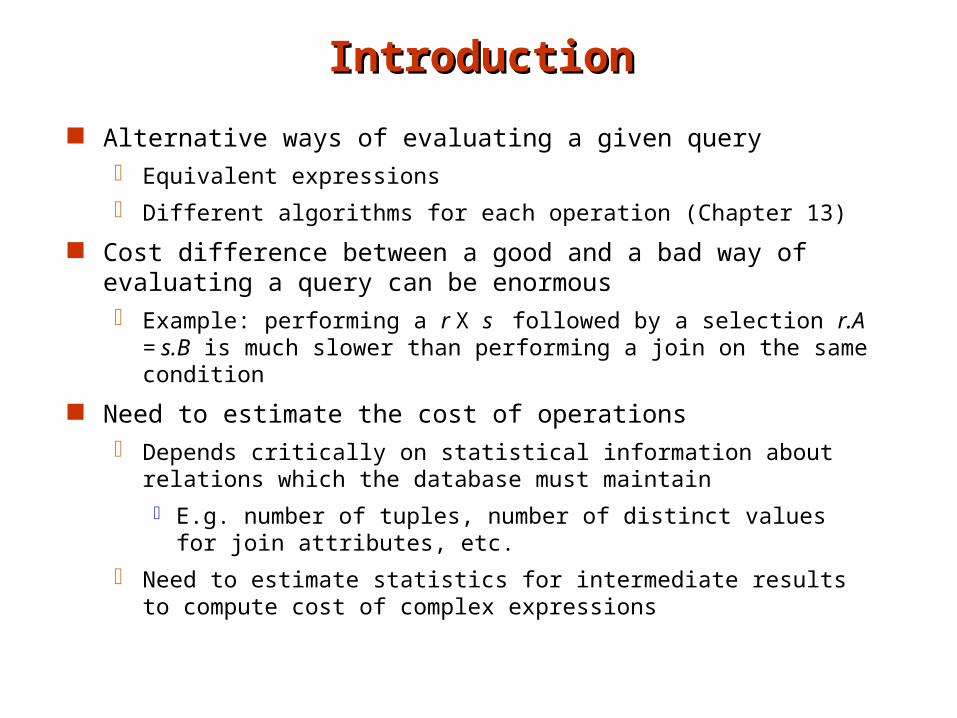
Alternative ways of evaluating a given query Equivalent expressions

Different algorithms for each operation (Chapter 13)

Cost difference between a good and a bad way of evaluating a query can be enormous Example: performing a r X s followed by a selection r.A = s.B is

much slower than performing a join on the same condition

Need to estimate the cost of operations Depends critically on statistical information about relations which the

database must maintain

E.g. number of tuples, number of distinct values for join attributes, etc.

Need to estimate statistics for intermediate results to compute cost of complex expressions

Introduction (Cont.)Introduction (Cont.)

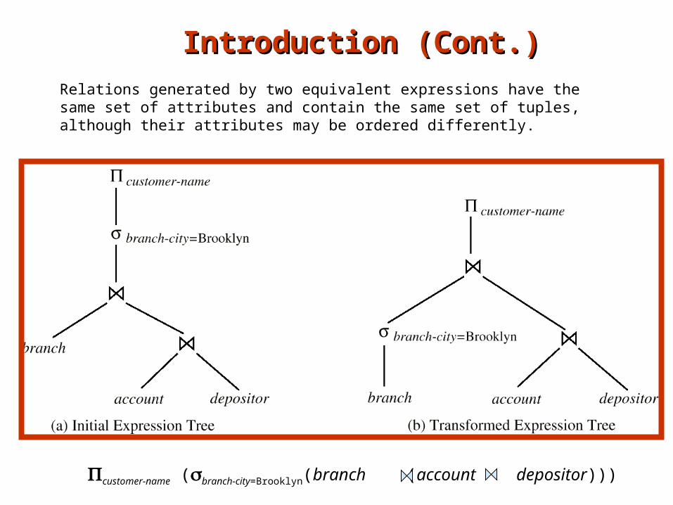
Relations generated by two equivalent expressions have the same set of attributes and contain the same set of tuples, although their attributes may be ordered differently.

customer-name (branch-city=Brooklyn(branch (account depositor)))

Introduction (Cont.)Introduction (Cont.)

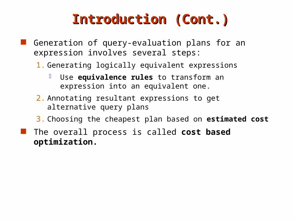
Generation of query-evaluation plans for an expression involves several steps:

1. Generating logically equivalent expressions

Use equivalence rules to transform an expression into an equivalent one.

2. Annotating resultant expressions to get alternative query plans

3. Choosing the cheapest plan based on estimated cost

The overall process is called cost based optimization.

Overview of chapterOverview of chapter

Statistical information for cost estimation

Equivalence rules

Cost-based optimization algorithm

Optimizing nested subqueries

Materialized views and view maintenance

Statistical Information for Cost Statistical Information for Cost EstimationEstimation

nr: number of tuples in a relation r.

br: number of blocks containing tuples of r.

sr: size of a tuple of r.

fr: blocking factor of r — i.e., the number of tuples of r that fit into one block.

V(A, r): number of distinct values that appear in r for attribute A; same as the size of A(r).

SC(A, r): selection cardinality of attribute A of relation r; average number of records that satisfy equality on A.

If tuples of r are stored together physically in a file, then:

rfrn

rb

Catalog Information about IndicesCatalog Information about Indices

fi: average fan-out of internal nodes of index i, for

tree-structured indices such as B+-trees.

HTi: number of levels in index i — i.e., the height of i.

For a balanced tree index (such as B+-tree) on attribute A of relation r, HTi = logfi(V(A,r)).

For a hash index, HTi is 1.

LBi: number of lowest-level index blocks in i — i.e, the

number of blocks at the leaf level of the index.

Measures of Query CostMeasures of Query Cost Recall that

Typically disk access is the predominant cost, and is also relatively easy to estimate.

The number of block transfers from disk is used as a measure of the actual cost of evaluation.

It is assumed that all transfers of blocks have the same cost.

Real life optimizers do not make this assumption, and distinguish between sequential and random disk access

We do not include cost to writing output to disk.

We refer to the cost estimate of algorithm A as EA

Selection Size EstimationSelection Size Estimation

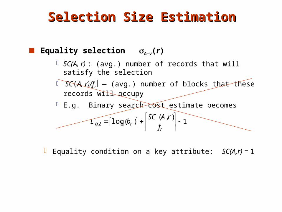
Equality selection A=v(r)

SC(A, r) : (avg.) number of records that will satisfy the selection

SC(A, r)/fr — (avg.) number of blocks that these records will occupy

E.g. Binary search cost estimate becomes

Equality condition on a key attribute: SC(A,r) = 1

1),(

)(log22

rra f

rASCbE

Selections Involving ComparisonsSelections Involving Comparisons

Selections of the form AV(r) (case of A V(r) is symmetric)

Let c denote the estimated number of tuples satisfying the condition. If min(A,r) and max(A,r) are available in catalog

C = 0 if v < min(A,r)

C =

In absence of statistical information c is assumed to be nr / 2.

),min(),max(

),min(.

rArA

rAvnr

Implementation of Complex SelectionsImplementation of Complex Selections

The selectivity of a condition i is the probability that a tuple in

the relation r satisfies i . If si is the number of satisfying tuples

in r, the selectivity of i is given by si /nr.

Conjunction: 1 2. . . n (r). The estimate for number of tuples in the result is:

Disjunction:1 2 . . . n (r). Estimated number of tuples:

Negation: (r). Estimated number of tuples:nr – size((r))

nr

nr n

sssn

. . . 21

)1(...)1()1(1 21

r

n

rrr n

s

n

s

n

sn

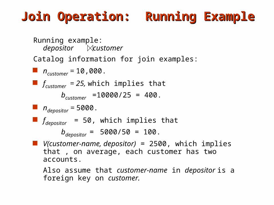
Join Operation: Running ExampleJoin Operation: Running Example

Running example: depositor customer

Catalog information for join examples:

ncustomer = 10,000.

fcustomer = 25, which implies that

bcustomer =10000/25 = 400.

ndepositor = 5000.

fdepositor = 50, which implies that

bdepositor = 5000/50 = 100.

V(customer-name, depositor) = 2500, which implies that , on average, each customer has two accounts.

Also assume that customer-name in depositor is a foreign key on customer.

Estimation of the Size of JoinsEstimation of the Size of Joins

The Cartesian product r x s contains nr .ns tuples; each tuple occupies sr + ss bytes.

If R S = , then r s is the same as r x s. If R S is a key for R, then a tuple of s will join with at most

one tuple from r therefore, the number of tuples in r s is no greater than the

number of tuples in s.

If R S in S is a foreign key in S referencing R, then the number of tuples in r s is exactly the same as the number of tuples in s.

The case for R S being a foreign key referencing S is symmetric.

In the example query depositor customer, customer-name in depositor is a foreign key of customer hence, the result has exactly ndepositor tuples, which is 5000

Estimation of the Size of Joins (Cont.)Estimation of the Size of Joins (Cont.)

If R S = {A} is not a key for R or S.If we assume that every tuple t in R produces tuples in R S, the number of tuples in R S is estimated to be:

If the reverse is true, the estimate obtained will be:

The lower of these two estimates is probably the more accurate one.

),( sAVnn sr

),( rAVnn sr

Estimation of the Size of Joins (Cont.)Estimation of the Size of Joins (Cont.)

Compute the size estimates for depositor customer without using information about foreign keys: V(customer-name, depositor) = 2500, and

V(customer-name, customer) = 10000

The two estimates are

5000 * 10000/2500 = 20,000 and

5000 * 10000/10000 = 5000

We choose the lower estimate, which in this case, is the same as our earlier computation using foreign keys.

Size Estimation for Other OperationsSize Estimation for Other Operations

Projection: estimated size of A(r) = V(A,r)

Aggregation : estimated size of AgF(r) = V(A,r)

Set operations For unions/intersections of selections on the same relation: rewrite

and use size estimate for selections

E.g. 1 (r) 2 (r) can be rewritten as 1 2 (r)

For operations on different relations:

estimated size of r s = size of r + size of s.

estimated size of r s = minimum size of r and size of s.

estimated size of r – s = r.

All the three estimates may be quite inaccurate, but provide upper bounds on the sizes.

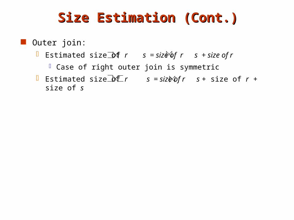
Size Estimation (Cont.)Size Estimation (Cont.)

Outer join: Estimated size of r s = size of r s + size of r

Case of right outer join is symmetric

Estimated size of r s = size of r s + size of r + size of s

Estimation of Number of Distinct ValuesEstimation of Number of Distinct Values

Selections: (r)

If forces A to take a specified value: V(A, (r)) = 1.

e.g., A = 3

If forces A to take on one of a specified set of values: V(A, (r)) = number of specified values.

(e.g., (A = 1 V A = 3 V A = 4 )),

If the selection condition is of the form A op restimated V(A, (r)) = V(A.r) * s

where s is the selectivity of the selection.

In all the other cases: use approximate estimate of min(V(A,r), n (r) )

More accurate estimate can be got using probability theory, but this one works fine generally

Estimation of Distinct Values (Cont.)Estimation of Distinct Values (Cont.)

Joins: r s

If all attributes in A are from r estimated V(A, r s) = min (V(A,r), n r s)

If A contains attributes A1 from r and A2 from s, then estimated V(A,r s) =

min(V(A1,r)*V(A2 – A1,s), V(A1 – A2,r)*V(A2,s), nr s)

More accurate estimate can be got using probability theory, but this one works fine generally

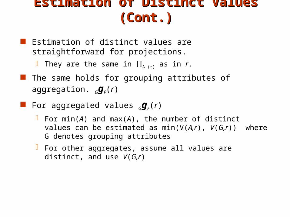
Estimation of Distinct Values (Cont.)Estimation of Distinct Values (Cont.)

Estimation of distinct values are straightforward for projections.

They are the same in A (r) as in r.

The same holds for grouping attributes of aggregation. GgF(r)

For aggregated values GgF(r)

For min(A) and max(A), the number of distinct values can be estimated as min(V(A,r), V(G,r)) where G denotes grouping attributes

For other aggregates, assume all values are distinct, and use V(G,r)

Transformation of Relational Transformation of Relational ExpressionsExpressions

Two relational algebra expressions are said to be equivalent if on every legal database instance the two expressions generate the same set of tuples Note: order of tuples is irrelevant

In SQL, inputs and outputs are multisets of tuples Two expressions in the multiset version of the relational algebra are

said to be equivalent if on every legal database instance the two expressions generate the same multiset of tuples

An equivalence rule says that expressions of two forms are equivalent Can replace expression of first form by second, or vice versa

Equivalence RulesEquivalence Rules

1. Conjunctive selection operations can be deconstructed into a sequence of individual selections.

2. Selection operations are commutative.

3. Only the last in a sequence of projection operations is needed, the others can be omitted.

4. Selections can be combined with Cartesian products and theta joins.

a. (E1 X E2) = E1 E2

b. 1(E1 2 E2) = E1 1 2 E2

))(())((1221EE

))(()(2121EE

)())))((((121EE ttntt

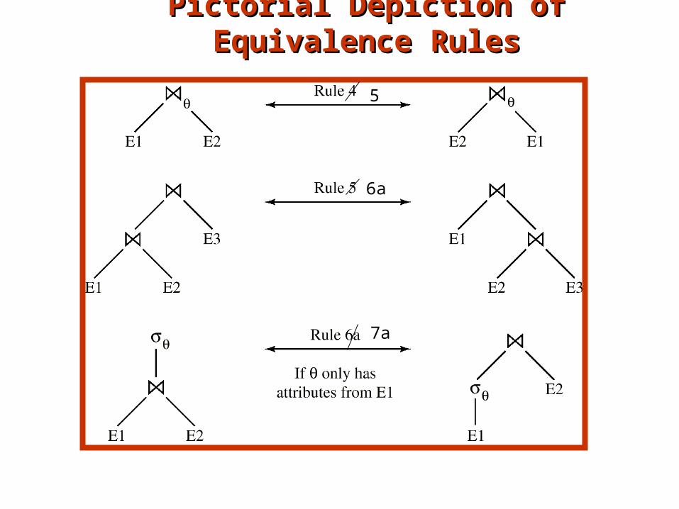
Pictorial Depiction of Equivalence RulesPictorial Depiction of Equivalence Rules

5

6a

7a

Equivalence Rules (Cont.)Equivalence Rules (Cont.)

5. Theta-join operations (and natural joins) are commutative.E1 E2 = E2 E1

6. (a) Natural join operations are associative:

(E1 E2) E3 = E1 (E2 E3)

(b) Theta joins are associative in the following manner:

(E1 1 E2) 2 3 E3 = E1 1 3 (E2 2 E3) where 2 involves attributes from only E2 and E3.

Equivalence Rules (Cont.)Equivalence Rules (Cont.)

7. The selection operation distributes over the theta join operation under the following two conditions:(a) When all the attributes in 0 involve only the attributes of one

of the expressions (E1) being joined.

0E1 E2) = (0(E1)) E2

(b) When 1 involves only the attributes of E1 and 2 involves only the attributes of E2.

1 E1 E2) = (1(E1)) ( (E2))

Equivalence Rules (Cont.)Equivalence Rules (Cont.)

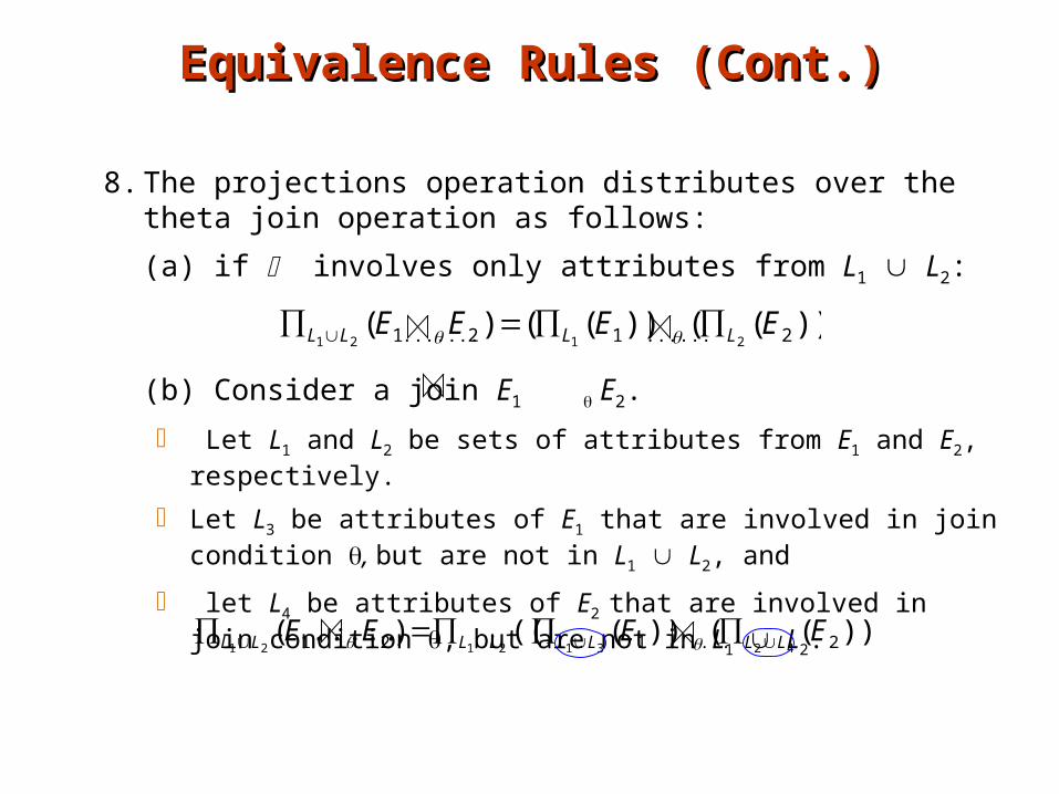
8. The projections operation distributes over the theta join operation as follows:

(a) if involves only attributes from L1 L2:

(b) Consider a join E1 E2.

Let L1 and L2 be sets of attributes from E1 and E2, respectively.

Let L3 be attributes of E1 that are involved in join condition , but are not in L1 L2, and

let L4 be attributes of E2 that are involved in join condition , but are not in L1 L2.

))(())(()( 2......12.......1 2121EEEE LLLL

)))(())((().....( 2......121 42312121EEEE LLLLLLLL

Equivalence Rules (Cont.)Equivalence Rules (Cont.)

9. The set operations union and intersection are commutative E1 E2 = E2 E1 E1 E2 = E2 E1

(set difference is not commutative).

10. Set union and intersection are associative.

(E1 E2) E3 = E1 (E2 E3) (E1 E2) E3 = E1 (E2 E3)

11. The selection operation distributes over , and –.

(E1 – E2) = (E1) – (E2)

and similarly for and in place of –

Also: (E1 – E2) = (E1) – E2

and similarly for in place of –, but not for

12. The projection operation distributes over union

L(E1 E2) = (L(E1)) (L(E2))

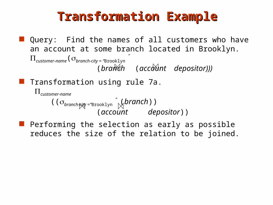
Transformation ExampleTransformation Example

Query: Find the names of all customers who have an account at some branch located in Brooklyn.customer-name(branch-city = “Brooklyn”

(branch (account depositor)))

Transformation using rule 7a. customer-name

((branch-city =“Brooklyn” (branch)) (account depositor))

Performing the selection as early as possible reduces the size of the relation to be joined.

Example with Multiple TransformationsExample with Multiple Transformations

Query: Find the names of all customers with an account at a Brooklyn branch whose account balance is over $1000.

customer-name((branch-city = “Brooklyn” balance > 1000

(branch (account depositor))) Transformation using join associativity (Rule 6a):

customer-name((branch-city = “Brooklyn” balance > 1000

(branch (account)) depositor) Second form provides an opportunity to apply the “perform

selections early” rule, resulting in the subexpression

branch-city = “Brooklyn” (branch) balance > 1000 (account)

Thus a sequence of transformations can be useful

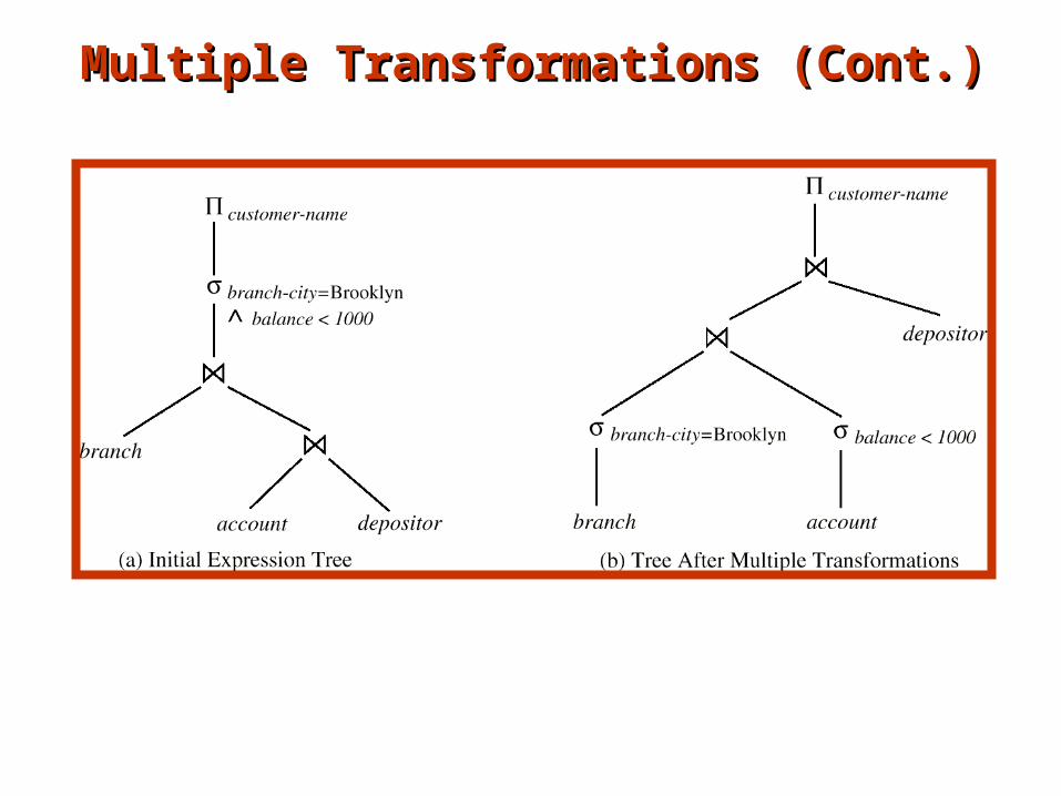
Multiple Transformations (Cont.)Multiple Transformations (Cont.)

Projection Operation ExampleProjection Operation Example

When we compute

(branch-city = “Brooklyn” (branch) account )

we obtain a relation whose schema is:(branch-name, branch-city, assets, account-number, balance)

Push projections using equivalence rules 8a and 8b; eliminate unneeded attributes from intermediate results to get: customer-name (( account-number ( (branch-city = “Brooklyn” (branch) account )) depositor)

customer-name((branch-city = “Brooklyn” (branch) account) depositor)

Join Ordering ExampleJoin Ordering Example

For all relations r1, r2, and r3,

(r1 r2) r3 = r1 (r2 r3 )

If r2 r3 is quite large and r1 r2 is small, we choose

(r1 r2) r3

so that we compute and store a smaller temporary relation.

Join Ordering Example (Cont.)Join Ordering Example (Cont.)

Consider the expression

customer-name ((branch-city = “Brooklyn” (branch)) account depositor)

Could compute account depositor first, and join result with

branch-city = “Brooklyn” (branch)but account depositor is likely to be a large relation.

Since it is more likely that only a small fraction of the bank’s customers have accounts in branches located in Brooklyn, it is better to compute

branch-city = “Brooklyn” (branch) account

first.

Enumeration of Equivalent ExpressionsEnumeration of Equivalent Expressions

Query optimizers use equivalence rules to systematically generate expressions equivalent to the given expression

Conceptually, generate all equivalent expressions by repeatedly executing the following step until no more expressions can be found: for each expression found so far, use all applicable equivalence rules,

and add newly generated expressions to the set of expressions found so far

The above approach is very expensive in space and time Space requirements reduced by sharing common subexpressions:

when E1 is generated from E2 by an equivalence rule, usually only the top level of the two are different, subtrees below are the same and can be shared E.g. when applying join associativity

Time requirements are reduced by not generating all expressions More details shortly

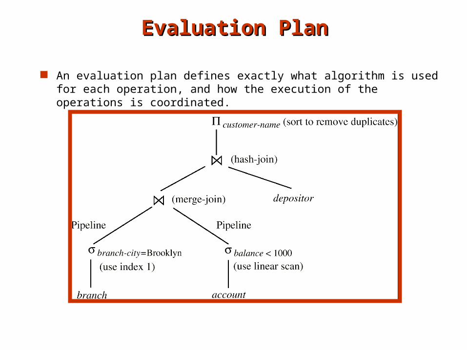
Evaluation PlanEvaluation Plan

An evaluation plan defines exactly what algorithm is used for each operation, and how the execution of the operations is coordinated.

Choice of Evaluation PlansChoice of Evaluation Plans

Must consider the interaction of evaluation techniques when choosing evaluation plans: choosing the cheapest algorithm for each operation independently may not yield best overall algorithm. E.g. merge-join may be costlier than hash-join, but may provide a sorted

output which reduces the cost for an outer level aggregation.

nested-loop join may provide opportunity for pipelining

Practical query optimizers incorporate elements of the following two broad approaches:

1. Search all the plans and choose the best plan in a cost-based fashion.

2. Uses heuristics to choose a plan.

Cost-Based OptimizationCost-Based Optimization

Consider finding the best join-order for r1 r2 . . . rn.

There are (2(n – 1))!/(n – 1)! different join orders for above expression. With n = 7, the number is 665280, with n = 10, the number is greater than 176 billion!

No need to generate all the join orders. Using dynamic programming, the least-cost join order for any subset of {r1, r2, . . . rn} is computed only once and stored for future use.

Dynamic Programming in OptimizationDynamic Programming in Optimization

To find best join tree for a set of n relations: To find best plan for a set S of n relations, consider all possible

plans of the form: S1 (S – S1) where S1 is any non-empty subset of S.

Recursively compute costs for joining subsets of S to find the cost of each plan. Choose the cheapest of the 2n – 1 alternatives.

When plan for any subset is computed, store it and reuse it when it is required again, instead of recomputing it

Dynamic programming

Join Order Optimization AlgorithmJoin Order Optimization Algorithm

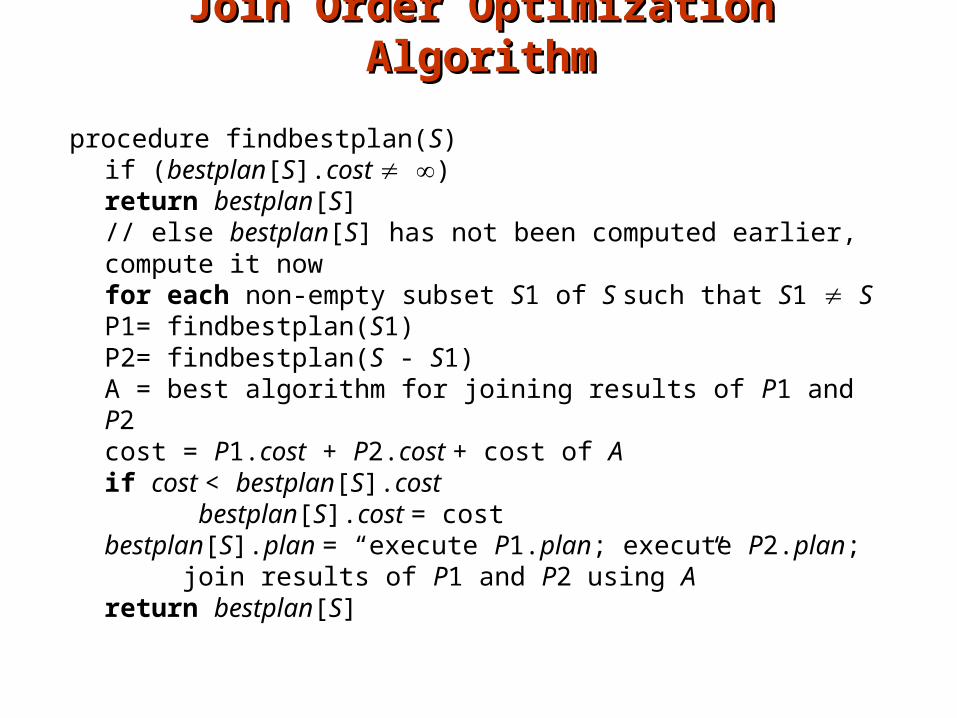
procedure findbestplan(S)if (bestplan[S].cost )

return bestplan[S]// else bestplan[S] has not been computed earlier, compute it nowfor each non-empty subset S1 of S such that S1 S

P1= findbestplan(S1)P2= findbestplan(S - S1)A = best algorithm for joining results of P1 and P2cost = P1.cost + P2.cost + cost of Aif cost < bestplan[S].cost

bestplan[S].cost = costbestplan[S].plan = “execute P1.plan; execute

P2.plan; join results of P1 and P2 using

A”return bestplan[S]

Left Deep Join TreesLeft Deep Join Trees

In left-deep join trees, the right-hand-side input for each join is a relation, not the result of an intermediate join.

Cost of OptimizationCost of Optimization

With dynamic programming time complexity of optimization with bushy trees is O(3n). With n = 10, this number is 59000 instead of 176 billion!

Space complexity is O(2n) To find best left-deep join tree for a set of n relations:

Consider n alternatives with one relation as right-hand side input and the other relations as left-hand side input.

Using (recursively computed and stored) least-cost join order for each alternative on left-hand-side, choose the cheapest of the n alternatives.

If only left-deep trees are considered, time complexity of finding best join order is O(n 2n) Space complexity remains at O(2n)

Cost-based optimization is expensive, but worthwhile for queries on large datasets (typical queries have small n, generally < 10)

Interesting Orders in Cost-Based OptimizationInteresting Orders in Cost-Based Optimization

Consider the expression (r1 r2 r3) r4 r5

An interesting sort order is a particular sort order of tuples that could be useful for a later operation.

Generating the result of r1 r2 r3 sorted on the attributes common with r4 or r5 may be useful, but generating it sorted on the attributes common only r1 and r2 is not useful.

Using merge-join to compute r1 r2 r3 may be costlier, but may provide an output sorted in an interesting order.

Not sufficient to find the best join order for each subset of the set of n given relations; must find the best join order for each subset, for each interesting sort order Simple extension of earlier dynamic programming algorithms

Usually, number of interesting orders is quite small and doesn’t affect time/space complexity significantly

Heuristic OptimizationHeuristic Optimization

Cost-based optimization is expensive, even with dynamic programming.

Systems may use heuristics to reduce the number of choices that must be made in a cost-based fashion.

Heuristic optimization transforms the query-tree by using a set of rules that typically (but not in all cases) improve execution performance: Perform selection early (reduces the number of tuples)

Perform projection early (reduces the number of attributes)

Perform most restrictive selection and join operations before other similar operations.

Some systems use only heuristics, others combine heuristics with partial cost-based optimization.

Steps in Typical Heuristic OptimizationSteps in Typical Heuristic Optimization

1. Deconstruct conjunctive selections into a sequence of single selection operations (Equiv. rule 1.).

2. Move selection operations down the query tree for the earliest possible execution (Equiv. rules 2, 7a, 7b, 11).

3. Execute first those selection and join operations that will produce the smallest relations (Equiv. rule 6).

4. Replace Cartesian product operations that are followed by a selection condition by join operations (Equiv. rule 4a).

5. Deconstruct and move as far down the tree as possible lists of projection attributes, creating new projections where needed (Equiv. rules 3, 8a, 8b, 12).

6. Identify those subtrees whose operations can be pipelined, and execute them using pipelining).

Structure of Query OptimizersStructure of Query Optimizers

The System R/Starburst optimizer considers only left-deep join orders. This reduces optimization complexity and generates plans amenable to pipelined evaluation.System R/Starburst also uses heuristics to push selections and projections down the query tree.

Heuristic optimization used in some versions of Oracle: Repeatedly pick “best” relation to join next

Starting from each of n starting points. Pick best among these.

For scans using secondary indices, some optimizers take into account the probability that the page containing the tuple is in the buffer.

Intricacies of SQL complicate query optimization E.g. nested subqueries

Structure of Query Optimizers (Cont.)Structure of Query Optimizers (Cont.)

Some query optimizers integrate heuristic selection and the generation of alternative access plans. System R and Starburst use a hierarchical procedure based on

the nested-block concept of SQL: heuristic rewriting followed by cost-based join-order optimization.

Even with the use of heuristics, cost-based query optimization imposes a substantial overhead.

This expense is usually more than offset by savings at query-execution time, particularly by reducing the number of slow disk accesses.

Optimizing Nested Subqueries**Optimizing Nested Subqueries** SQL conceptually treats nested subqueries in the where clause as

functions that take parameters and return a single value or set of values Parameters are variables from outer level query that are used in the

nested subquery; such variables are called correlation variables

E.g.select customer-namefrom borrowerwhere exists (select *

from depositor where depositor.customer-name =

borrower.customer-name)

Conceptually, nested subquery is executed once for each tuple in the cross-product generated by the outer level from clause Such evaluation is called correlated evaluation Note: other conditions in where clause may be used to compute a join

(instead of a cross-product) before executing the nested subquery

Optimizing Nested Subqueries (Cont.)Optimizing Nested Subqueries (Cont.)

Correlated evaluation may be quite inefficient since a large number of calls may be made to the nested query

there may be unnecessary random I/O as a result

SQL optimizers attempt to transform nested subqueries to joins where possible, enabling use of efficient join techniques

E.g.: earlier nested query can be rewritten as select customer-namefrom borrower, depositorwhere depositor.customer-name = borrower.customer-name Note: above query doesn’t correctly deal with duplicates, can be

modified to do so as we will see

In general, it is not possible/straightforward to move the entire nested subquery from clause into the outer level query from clause A temporary relation is created instead, and used in body of outer

level query

Optimizing Nested Subqueries (Cont.)Optimizing Nested Subqueries (Cont.)In general, SQL queries of the form below can be rewritten as shown Rewrite: select …

from L1

where P1 and exists (select * from L2

where P2)

To: create table t1 as select distinct V from L2

where P21

select … from L1, t1 where P1 and P2

2

P21 contains predicates in P2 that do not involve any correlation variables

P22 reintroduces predicates involving correlation variables, with

relations renamed appropriately V contains all attributes used in predicates with correlation variables

Optimizing Nested Subqueries (Cont.)Optimizing Nested Subqueries (Cont.)

In our example, the original nested query would be transformed to create table t1 as select distinct customer-name from depositor select customer-name from borrower, t1

where t1.customer-name = borrower.customer-name The process of replacing a nested query by a query with a join

(possibly with a temporary relation) is called decorrelation. Decorrelation is more complicated when

the nested subquery uses aggregation, or when the result of the nested subquery is used to test for equality, or when the condition linking the nested subquery to the other

query is not exists, and so on.

Materialized Views**Materialized Views**

A materialized view is a view whose contents are computed and stored.

Consider the viewcreate view branch-total-loan(branch-name, total-loan) asselect branch-name, sum(amount)from loangroupby branch-name

Materializing the above view would be very useful if the total loan amount is required frequently Saves the effort of finding multiple tuples and adding up their

amounts

Materialized View MaintenanceMaterialized View Maintenance

The task of keeping a materialized view up-to-date with the underlying data is known as materialized view maintenance

Materialized views can be maintained by recomputation on every update

A better option is to use incremental view maintenance Changes to database relations are used to compute changes to

materialized view, which is then updated

View maintenance can be done by Manually defining triggers on insert, delete, and update of each

relation in the view definition

Manually written code to update the view whenever database relations are updated

Supported directly by the database

Incremental View MaintenanceIncremental View Maintenance

The changes (inserts and deletes) to a relation or expressions are referred to as its differential

Set of tuples inserted to and deleted from r are denoted ir and dr

To simplify our description, we only consider inserts and deletes We replace updates to a tuple by deletion of the tuple followed by

insertion of the update tuple

We describe how to compute the change to the result of each relational operation, given changes to its inputs

We then outline how to handle relational algebra expressions

Join OperationJoin Operation

Consider the materialized view v = r s and an update to r

Let rold and rnew denote the old and new states of relation r

Consider the case of an insert to r:

We can write rnew s as (rold ir) s

And rewrite the above to (rold s) (ir s)

But (rold s) is simply the old value of the materialized view, so the

incremental change to the view is just ir s

Thus, for inserts vnew = vold (ir s)

Similarly for deletes vnew = vold – (dr s)

Selection and Projection OperationsSelection and Projection Operations

Selection: Consider a view v = (r). vnew = vold (ir) vnew = vold - (dr)

Projection is a more difficult operation R = (A,B), and r(R) = { (a,2), (a,3)}

A(r) has a single tuple (a).

If we delete the tuple (a,2) from r, we should not delete the tuple (a) from A(r), but if we then delete (a,3) as well, we should delete the tuple

For each tuple in a projection A(r) , we will keep a count of how many times it was derived On insert of a tuple to r, if the resultant tuple is already in A(r) we

increment its count, else we add a new tuple with count = 1 On delete of a tuple from r, we decrement the count of the

corresponding tuple in A(r)

if the count becomes 0, we delete the tuple from A(r)

Aggregation OperationsAggregation Operations

count : v = Agcount(B)(r).

When a set of tuples ir is inserted

For each tuple r in ir, if the corresponding group is already present in v, we increment its count, else we add a new tuple with count = 1

When a set of tuples dr is deleted

for each tuple t in ir.we look for the group t.A in v, and subtract 1 from the count for the group.

– If the count becomes 0, we delete from v the tuple for the group t.A

sum: v = Agsum (B)(r)

We maintain the sum in a manner similar to count, except we add/subtract the B value instead of adding/subtracting 1 for the count

Additionally we maintain the count in order to detect groups with no tuples. Such groups are deleted from v Cannot simply test for sum = 0 (why?)

To handle the case of avg, we maintain the sum and count aggregate values separately, and divide at the end

Aggregate Operations (Cont.)Aggregate Operations (Cont.)

min, max: v = Agmin (B) (r).

Handling insertions on r is straightforward.

Maintaining the aggregate values min and max on deletions may be more expensive. We have to look at the other tuples of r that are in the same group to find the new minimum

Other OperationsOther Operations

Set intersection: v = r s when a tuple is inserted in r we check if it is present in s, and if so

we add it to v.

If the tuple is deleted from r, we delete it from the intersection if it is present.

Updates to s are symmetric

The other set operations, union and set difference are handled in a similar fashion.

Outer joins are handled in much the same way as joins but with some extra work we leave details to you.

Handling ExpressionsHandling Expressions

To handle an entire expression, we derive expressions for computing the incremental change to the result of each sub-expressions, starting from the smallest sub-expressions.

E.g. consider E1 E2 where each of E1 and E2 may be a complex expression

Suppose the set of tuples to be inserted into E1 is given by D1

Computed earlier, since smaller sub-expressions are handled first

Then the set of tuples to be inserted into E1 E2 is given by D1 E2

This is just the usual way of maintaining joins

Query Optimization and Materialized Query Optimization and Materialized ViewsViews

Rewriting queries to use materialized views: A materialized view v = r s is available

A user submits a query r s t

We can rewrite the query as v t

Whether to do so depends on cost estimates for the two alternative

Replacing a use of a materialized view by the view definition: A materialized view v = r s is available, but without any index on it

User submits a query A=10(v).

Suppose also that s has an index on the common attribute B, and r has an index on attribute A.

The best plan for this query may be to replace v by r s, which can lead to the query plan A=10(r) s

Query optimizer should be extended to consider all above alternatives and choose the best overall plan

Materialized View SelectionMaterialized View Selection

Materialized view selection: “What is the best set of views to materialize?”. This decision must be made on the basis of the system workload

Indices are just like materialized views, problem of index selection is closely related, to that of materialized view selection, although it is simpler.

Some database systems, provide tools to help the database administrator with index and materialized view selection.

End of ChapterEnd of Chapter

(Extra slides with details of selection cost estimation follow)

Selection Cost Estimate ExampleSelection Cost Estimate Example

Number of blocks is baccount = 500: 10,000 tuples in the relation; each block holds 20 tuples.

Assume account is sorted on branch-name. V(branch-name,account) is 50

10000/50 = 200 tuples of the account relation pertain to Perryridge branch

200/20 = 10 blocks for these tuples

A binary search to find the first record would take log2(500) = 9 block accesses

Total cost of binary search is 9 + 10 -1 = 18 block accesses (versus 500 for linear scan)

branch-name = “Perryridge”(account)

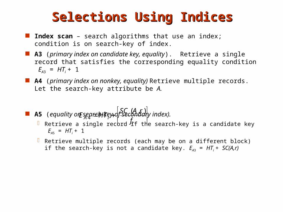
Selections Using IndicesSelections Using Indices Index scan – search algorithms that use an index; condition is on

search-key of index.

A3 (primary index on candidate key, equality). Retrieve a single record that satisfies the corresponding equality condition EA3 = HTi + 1

A4 (primary index on nonkey, equality) Retrieve multiple records. Let the search-key attribute be A.

A5 (equality on search-key of secondary index). Retrieve a single record if the search-key is a candidate key

EA5 = HTi + 1

Retrieve multiple records (each may be on a different block) if the search-key is not a candidate key. EA3 = HTi + SC(A,r)

riA f

rASCHTE

),(4

Cost Estimate Example (Indices)Cost Estimate Example (Indices)

Since V(branch-name, account) = 50, we expect that 10000/50 = 200 tuples of the account relation pertain to the Perryridge branch.

Since the index is a clustering index, 200/20 = 10 block reads are required to read the account tuples.

Several index blocks must also be read. If B+-tree index stores 20 pointers per node, then the B+-tree index must have between 3 and 5 leaf nodes and the entire tree has a depth of 2. Therefore, 2 index blocks must be read.

This strategy requires 12 total block reads.

Consider the query is branch-name = “Perryridge”(account), with the primary index on branch-name.

Selections Involving ComparisonsSelections Involving Comparisons

A6 (primary index, comparison). The cost estimate is:

where c is the estimated number of tuples satisfying the condition. In absence of statistical information c is assumed to be nr/2.

A7 (secondary index, comparison). The cost estimate:

where c is defined as before. (Linear file scan may be cheaper if c is large!).

selections of the form AV(r) or A V(r) by using a linear file scan or binary search, or by using indices in the following ways:

riAB f

cHTE

cn

cLBHTE

r

iiA 7

Example of Cost Estimate for Complex Example of Cost Estimate for Complex SelectionSelection

Consider a selection on account with the following condition: where branch-name = “Perryridge” and balance = 1200

Consider using algorithm A8: The branch-name index is clustering, and if we use it the cost

estimate is 12 block reads (as we saw before).

The balance index is non-clustering, and V(balance, account = 500, so the selection would retrieve 10,000/500 = 20 accounts. Adding the index block reads, gives a cost estimate of 22 block reads.

Thus using branch-name index is preferable, even though its condition is less selective.

If both indices were non-clustering, it would be preferable to use the balance index.

Example (Cont.)Example (Cont.)

Consider using algorithm A10:

Use the index on balance to retrieve set S1 of pointers to records with balance = 1200.

Use index on branch-name to retrieve-set S2 of pointers to records with branch-name = Perryridge”.

S1 S2 = set of pointers to records with branch-name = “Perryridge” and balance = 1200.

The number of pointers retrieved (20 and 200), fit into a single leaf page; we read four index blocks to retrieve the two sets of pointers and compute their intersection.

Estimate that one tuple in 50 * 500 meets both conditions. Since naccount = 10000, conservatively overestimate that S1 S2 contains one pointer.

The total estimated cost of this strategy is five block reads.