Chapter 14 · Fundamentals of Multimedia, Chapter 14 14.2 MPEG Audio MPEG audio compression takes...
42
Fundamentals of Multimedia, Chapter 14 Chapter 14 MPEG Audio Compression 14.1 Psychoacoustics 14.2 MPEG Audio 14.3 Other Commercial Audio Codecs 14.4 The Future: MPEG-7 and MPEG-21 14.5 Further Exploration 1 Li & Drew c Prentice Hall 2003
Transcript of Chapter 14 · Fundamentals of Multimedia, Chapter 14 14.2 MPEG Audio MPEG audio compression takes...
Fundamentals of Multimedia, Chapter 14
Chapter 14MPEG Audio Compression
14.1 Psychoacoustics
14.2 MPEG Audio
14.3 Other Commercial Audio Codecs
14.4 The Future: MPEG-7 and MPEG-21
14.5 Further Exploration
1 Li & Drew c©Prentice Hall 2003
Fundamentals of Multimedia, Chapter 14
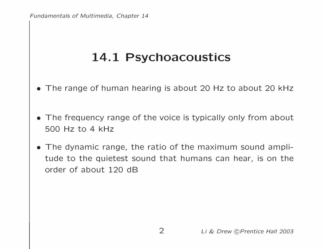
14.1 Psychoacoustics
• The range of human hearing is about 20 Hz to about 20 kHz
• The frequency range of the voice is typically only from about
500 Hz to 4 kHz
• The dynamic range, the ratio of the maximum sound ampli-
tude to the quietest sound that humans can hear, is on the
order of about 120 dB
2 Li & Drew c©Prentice Hall 2003
Fundamentals of Multimedia, Chapter 14
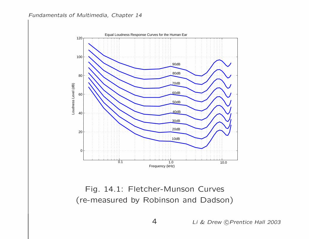
Equal-Loudness Relations
• Fletcher-Munson Curves
– Equal loudness curves that display the relationship be-
tween perceived loudness (“Phons”, in dB) for a given
stimulus sound volume (“Sound Pressure Level”, also in
dB), as a function of frequency
• Fig. 14.1 shows the ear’s perception of equal louness:
– The bottom curve shows what level of pure tone stimulus
is required to produce the perception of a 10 dB sound
– All the curves are arranged so that the perceived loudness
level gives the same loudness as for that loudness level of
a pure tone at 1 kHz
3 Li & Drew c©Prentice Hall 2003
Fundamentals of Multimedia, Chapter 14
0
20
40
60
80
100
120Equal Loudness Response Curves for the Human Ear
Frequency (kHz)
Loud
ness
Lev
el (
dB)
10dB
20dB
40dB
50dB
60dB
70dB
30dB
80dB
90dB
1.0 10.0 0.1
Fig. 14.1: Fletcher-Munson Curves
(re-measured by Robinson and Dadson)
4 Li & Drew c©Prentice Hall 2003
Fundamentals of Multimedia, Chapter 14
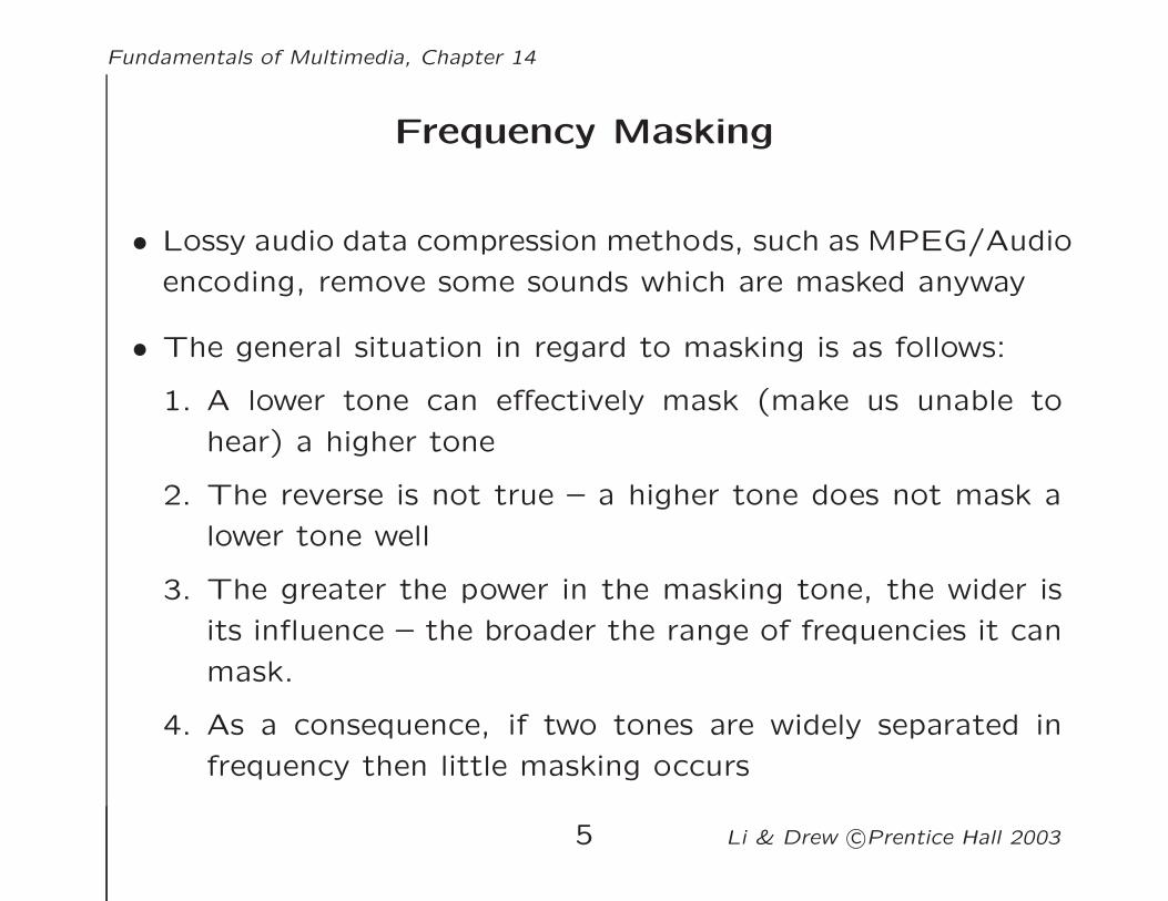
Frequency Masking
• Lossy audio data compression methods, such as MPEG/Audio
encoding, remove some sounds which are masked anyway
• The general situation in regard to masking is as follows:
1. A lower tone can effectively mask (make us unable to
hear) a higher tone
2. The reverse is not true – a higher tone does not mask a
lower tone well
3. The greater the power in the masking tone, the wider is
its influence – the broader the range of frequencies it can
mask.
4. As a consequence, if two tones are widely separated in
frequency then little masking occurs
5 Li & Drew c©Prentice Hall 2003
Fundamentals of Multimedia, Chapter 14
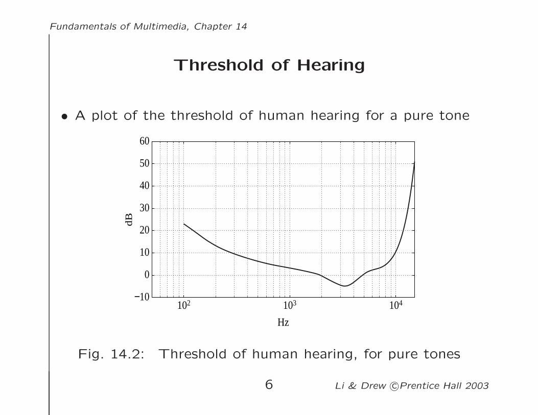
Threshold of Hearing
• A plot of the threshold of human hearing for a pure tone
102 103 104−10
0
10
20
30
40
50
60
Hz
dB
Fig. 14.2: Threshold of human hearing, for pure tones
6 Li & Drew c©Prentice Hall 2003
Fundamentals of Multimedia, Chapter 14
Threshold of Hearing (cont’d)
• The threshold of hearing curve: if a sound is above the dB
level shown then the sound is audible
• Turning up a tone so that it equals or surpasses the curve
means that we can then distinguish the sound
• An approximate formula exists for this curve:
Threshold(f) = 3.64(f/1000)−0.8 − 6.5 e−0.6(f/1000−3.3)2
+ 10−3(f/1000)4
(14.1)
– The threshold units are dB; the frequency for the origin
(0,0) in formula (14.1) is 2,000 Hz: Threshold(f) = 0 at
f =2 kHz
7 Li & Drew c©Prentice Hall 2003
Fundamentals of Multimedia, Chapter 14
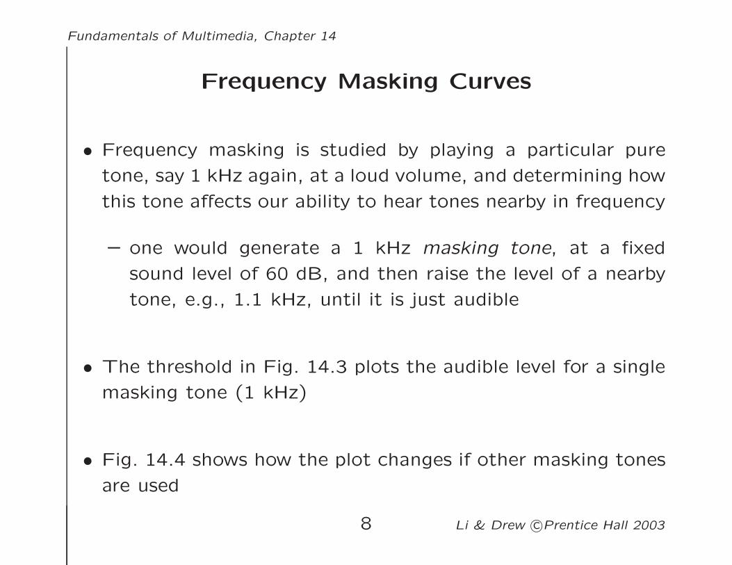
Frequency Masking Curves
• Frequency masking is studied by playing a particular pure
tone, say 1 kHz again, at a loud volume, and determining how
this tone affects our ability to hear tones nearby in frequency
– one would generate a 1 kHz masking tone, at a fixed
sound level of 60 dB, and then raise the level of a nearby
tone, e.g., 1.1 kHz, until it is just audible
• The threshold in Fig. 14.3 plots the audible level for a single
masking tone (1 kHz)
• Fig. 14.4 shows how the plot changes if other masking tones
are used
8 Li & Drew c©Prentice Hall 2003

Fundamentals of Multimedia, Chapter 14
0 1 2 3 4 5 6 7 8 9 10 11 12 1314 15−10
0
10
20
30
40
50
60
70
Frequency (kHz)
dB
Audible tone
Inaudible tone
Fig. 14.3: Effect on threshold for 1 kHz masking tone
9 Li & Drew c©Prentice Hall 2003
Fundamentals of Multimedia, Chapter 14
0 1 2 3 4 5 6 7 8 9 10 11 12 13 14 15−10
0
10
20
30
40
50
60
70
Frequency (kHz)
dB1 4 8
Fig. 14.4: Effect of masking tone at three different frequencies
10 Li & Drew c©Prentice Hall 2003
Fundamentals of Multimedia, Chapter 14
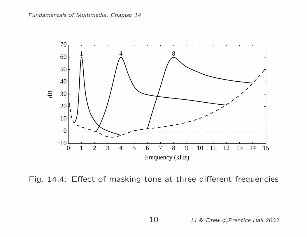
Critical Bands
• Critical bandwidth represents the ear’s resolving power for
simultaneous tones or partials
– At the low-frequency end, a critical band is less than
100 Hz wide, while for high frequencies the width can
be greater than 4 kHz
• Experiments indicate that the critical bandwidth:
– for masking frequencies < 500 Hz: remains approximately
constant in width ( about 100 Hz)
– for masking frequencies > 500 Hz: increases approxi-
mately linearly with frequency
11 Li & Drew c©Prentice Hall 2003
Fundamentals of Multimedia, Chapter 14
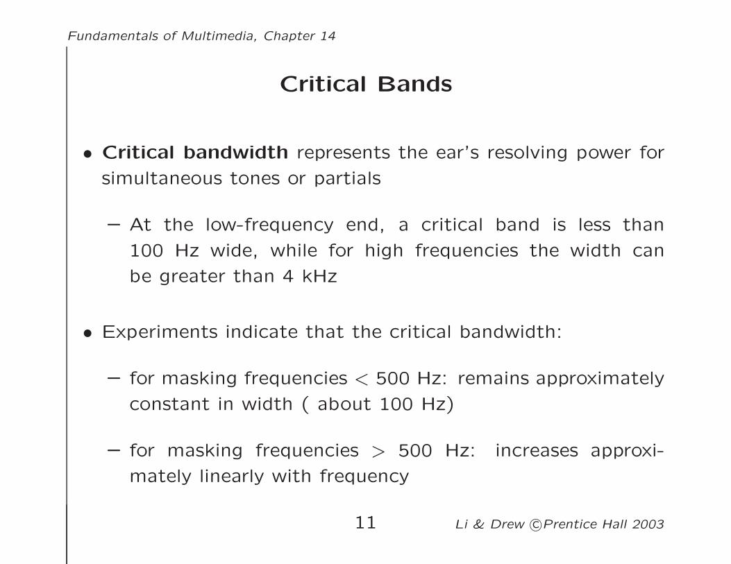
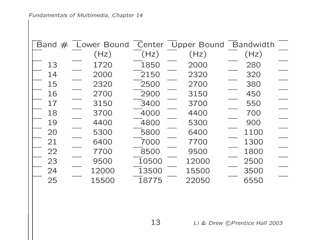
Table 14.1 25-Critical Bands and Bandwidth
Band # Lower Bound Center Upper Bound Bandwidth(Hz) (Hz) (Hz) (Hz)
1 - 50 100 -2 100 150 200 1003 200 250 300 1004 300 350 400 1005 400 450 510 1106 510 570 630 1207 630 700 770 1408 770 840 920 1509 920 1000 1080 16010 1080 1170 1270 19011 1270 1370 1480 21012 1480 1600 1720 240
12 Li & Drew c©Prentice Hall 2003
Fundamentals of Multimedia, Chapter 14
Band # Lower Bound Center Upper Bound Bandwidth(Hz) (Hz) (Hz) (Hz)
13 1720 1850 2000 28014 2000 2150 2320 32015 2320 2500 2700 38016 2700 2900 3150 45017 3150 3400 3700 55018 3700 4000 4400 70019 4400 4800 5300 90020 5300 5800 6400 110021 6400 7000 7700 130022 7700 8500 9500 180023 9500 10500 12000 250024 12000 13500 15500 350025 15500 18775 22050 6550
13 Li & Drew c©Prentice Hall 2003
Fundamentals of Multimedia, Chapter 14
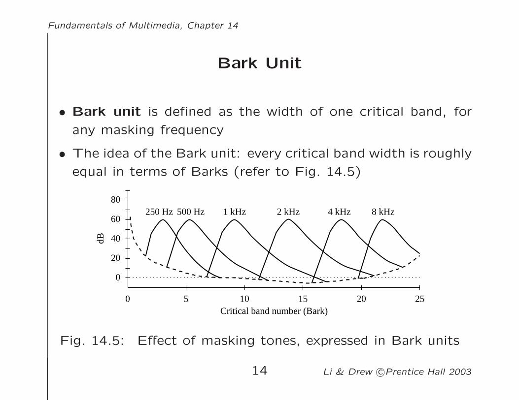
Bark Unit
• Bark unit is defined as the width of one critical band, for
any masking frequency
• The idea of the Bark unit: every critical band width is roughly
equal in terms of Barks (refer to Fig. 14.5)
250 Hz
0
20
40
60500 Hz 1 kHz 8 kHz4 kHz2 kHz
Critical band number (Bark)
dB
0 252015105
80
Fig. 14.5: Effect of masking tones, expressed in Bark units
14 Li & Drew c©Prentice Hall 2003
Fundamentals of Multimedia, Chapter 14
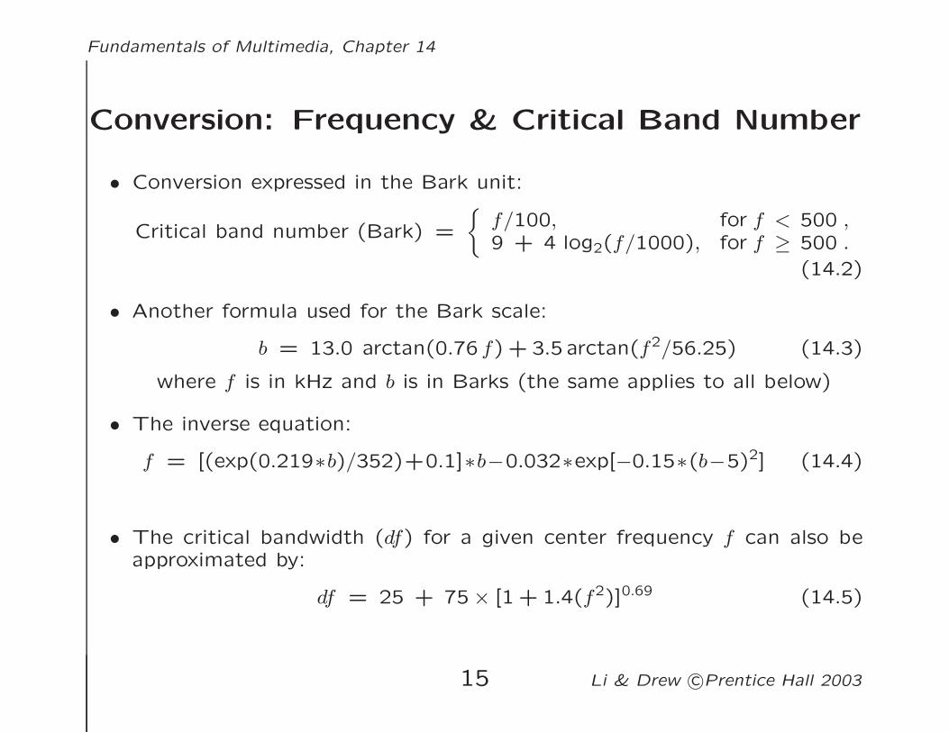
Conversion: Frequency & Critical Band Number
• Conversion expressed in the Bark unit:
Critical band number (Bark) =
{f/100, for f < 500 ,9 + 4 log2(f/1000), for f ≥ 500 .
(14.2)
• Another formula used for the Bark scale:
b = 13.0 arctan(0.76 f) + 3.5arctan(f2/56.25) (14.3)
where f is in kHz and b is in Barks (the same applies to all below)
• The inverse equation:
f = [(exp(0.219∗b)/352)+0.1]∗b−0.032∗exp[−0.15∗(b−5)2] (14.4)
• The critical bandwidth (df) for a given center frequency f can also beapproximated by:
df = 25 + 75× [1 + 1.4(f2)]0.69 (14.5)
15 Li & Drew c©Prentice Hall 2003
Fundamentals of Multimedia, Chapter 14
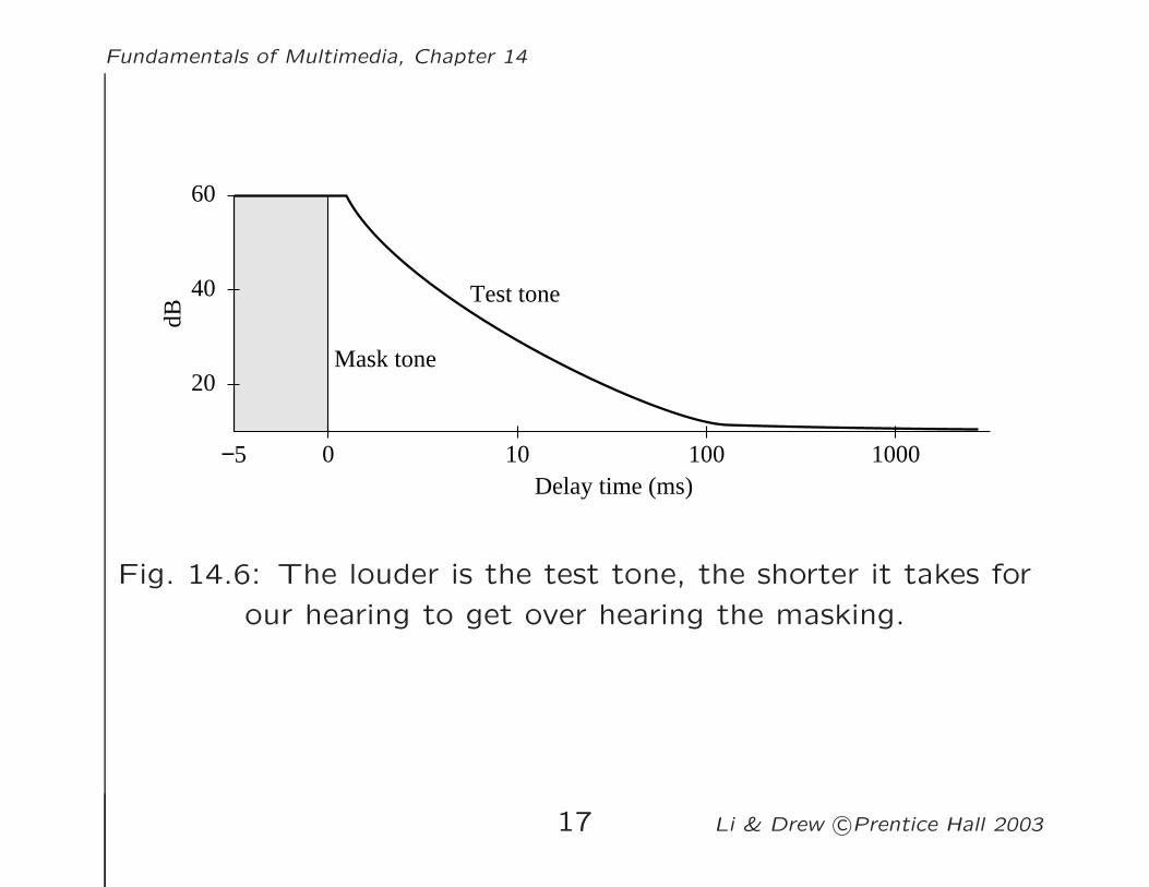
Temporal Masking
• Phenomenon: any loud tone will cause the hearing receptors
in the inner ear to become saturated and require time to
recover
• The following figures show the results of Masking experi-
ments:
16 Li & Drew c©Prentice Hall 2003
Fundamentals of Multimedia, Chapter 14
100Delay time (ms)
dB
Test tone
Mask tone
60
40
20
1000100−5
Fig. 14.6: The louder is the test tone, the shorter it takes for
our hearing to get over hearing the masking.
17 Li & Drew c©Prentice Hall 2003
Fundamentals of Multimedia, Chapter 14
0
0.01
0.02
0.03 0
4
6
8−10
0
10
20
30
40
50
60
Frequency
Time
Leve
l (dB
)
Tones below surfaceare inaudible
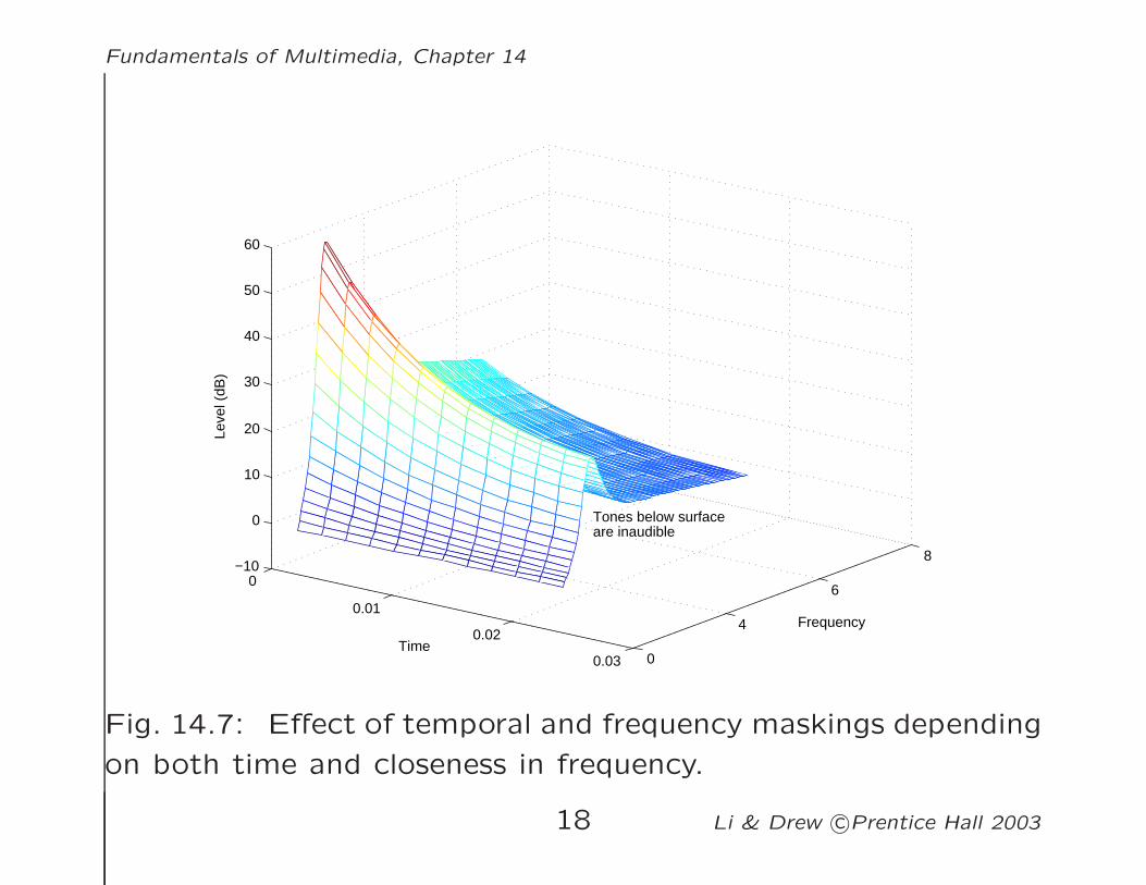
Fig. 14.7: Effect of temporal and frequency maskings depending
on both time and closeness in frequency.
18 Li & Drew c©Prentice Hall 2003
Fundamentals of Multimedia, Chapter 14
10
dB60
40
20
Delay time (ms)1000 5 50
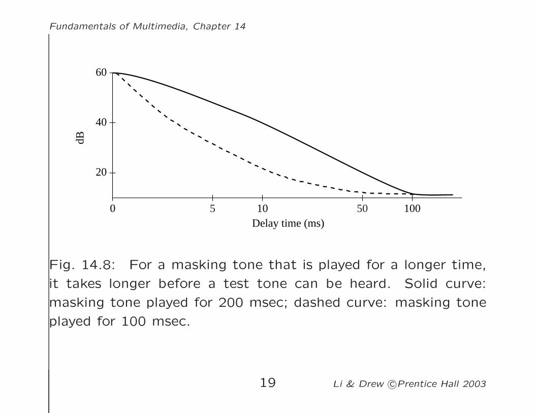
Fig. 14.8: For a masking tone that is played for a longer time,
it takes longer before a test tone can be heard. Solid curve:
masking tone played for 200 msec; dashed curve: masking tone
played for 100 msec.
19 Li & Drew c©Prentice Hall 2003
Fundamentals of Multimedia, Chapter 14
14.2 MPEG Audio
• MPEG audio compression takes advantage of psychoa-
coustic models, constructing a large multi-dimensional lookup
table to transmit masked frequency components using fewer
bits
• MPEG Audio Overview
1. Applies a filter bank to the input to break it into its fre-
quency components
2. In parallel, a psychoacoustic model is applied to the data
for bit allocation block
3. The number of bits allocated are used to quantize the
info from the filter bank – providing the compression
20 Li & Drew c©Prentice Hall 2003
Fundamentals of Multimedia, Chapter 14
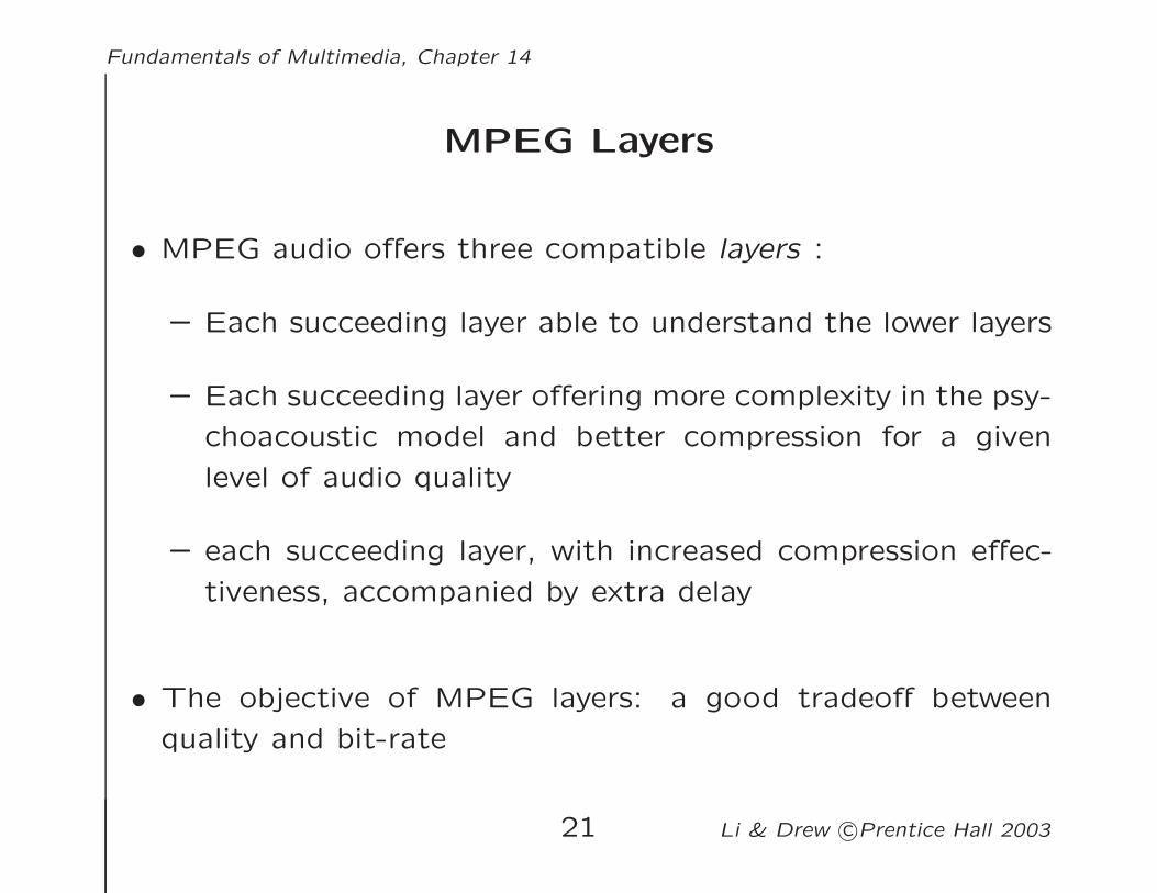
MPEG Layers
• MPEG audio offers three compatible layers :
– Each succeeding layer able to understand the lower layers
– Each succeeding layer offering more complexity in the psy-
choacoustic model and better compression for a given
level of audio quality
– each succeeding layer, with increased compression effec-
tiveness, accompanied by extra delay
• The objective of MPEG layers: a good tradeoff between
quality and bit-rate
21 Li & Drew c©Prentice Hall 2003
Fundamentals of Multimedia, Chapter 14
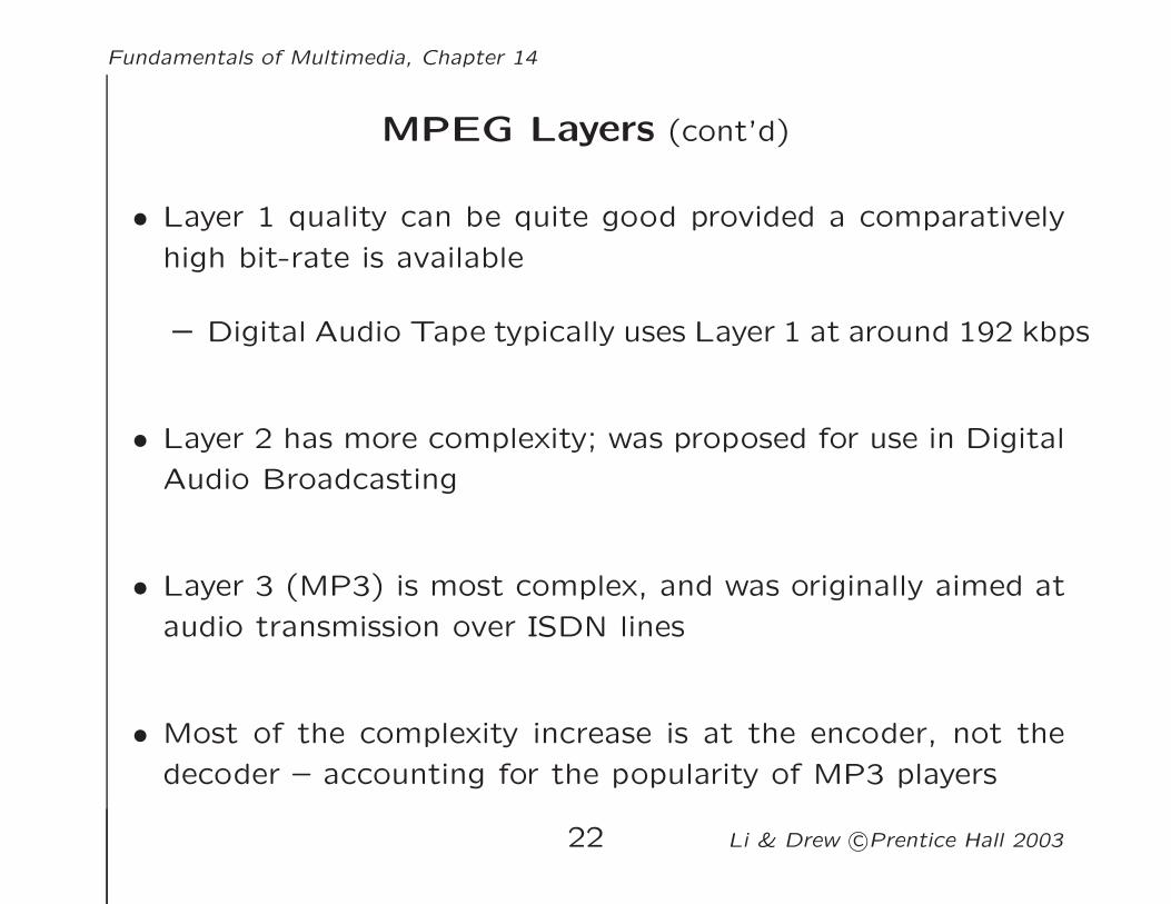
MPEG Layers (cont’d)
• Layer 1 quality can be quite good provided a comparatively
high bit-rate is available
– Digital Audio Tape typically uses Layer 1 at around 192 kbps
• Layer 2 has more complexity; was proposed for use in Digital
Audio Broadcasting
• Layer 3 (MP3) is most complex, and was originally aimed at
audio transmission over ISDN lines
• Most of the complexity increase is at the encoder, not the
decoder – accounting for the popularity of MP3 players
22 Li & Drew c©Prentice Hall 2003
Fundamentals of Multimedia, Chapter 14
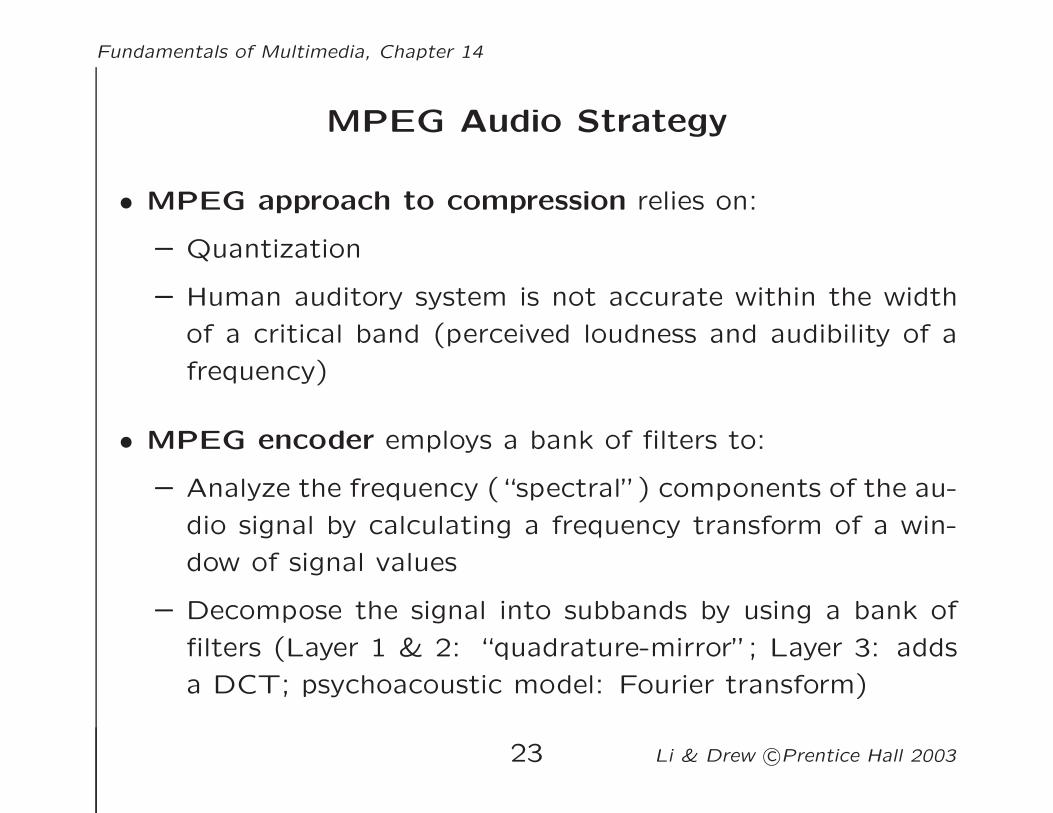
MPEG Audio Strategy
• MPEG approach to compression relies on:
– Quantization
– Human auditory system is not accurate within the width
of a critical band (perceived loudness and audibility of a
frequency)
• MPEG encoder employs a bank of filters to:
– Analyze the frequency (“spectral”) components of the au-
dio signal by calculating a frequency transform of a win-
dow of signal values
– Decompose the signal into subbands by using a bank of
filters (Layer 1 & 2: “quadrature-mirror”; Layer 3: adds
a DCT; psychoacoustic model: Fourier transform)
23 Li & Drew c©Prentice Hall 2003
Fundamentals of Multimedia, Chapter 14
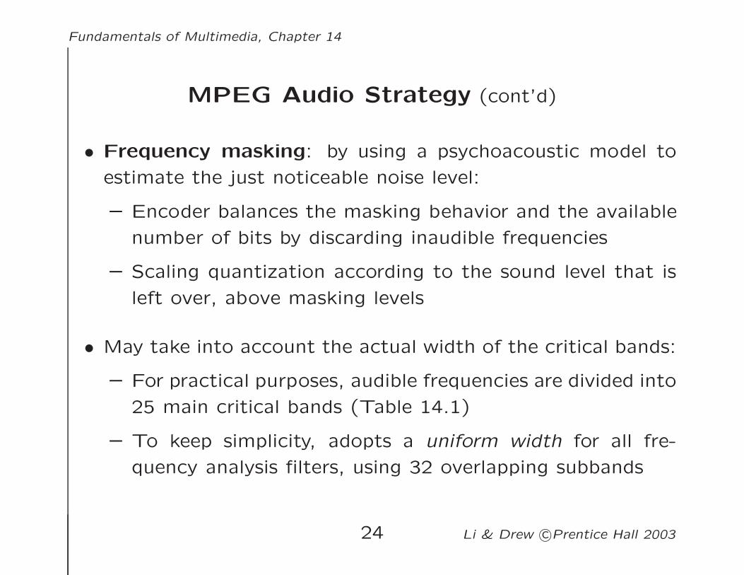
MPEG Audio Strategy (cont’d)
• Frequency masking: by using a psychoacoustic model to
estimate the just noticeable noise level:
– Encoder balances the masking behavior and the available
number of bits by discarding inaudible frequencies
– Scaling quantization according to the sound level that is
left over, above masking levels
• May take into account the actual width of the critical bands:
– For practical purposes, audible frequencies are divided into
25 main critical bands (Table 14.1)
– To keep simplicity, adopts a uniform width for all fre-
quency analysis filters, using 32 overlapping subbands
24 Li & Drew c©Prentice Hall 2003
Fundamentals of Multimedia, Chapter 14
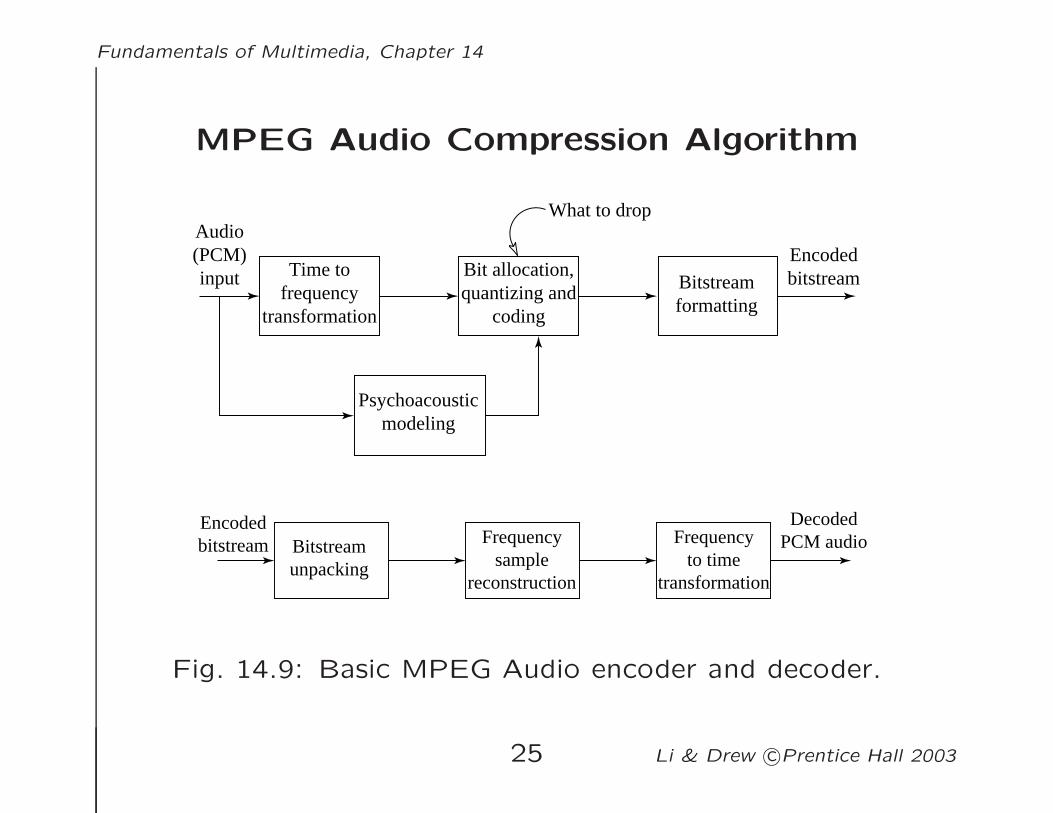
MPEG Audio Compression Algorithm
What to dropAudio(PCM)input
Psychoacousticmodeling
Bit allocation,quantizing and
coding
Bitstreamformatting
Time tofrequency
transformation
Encodedbitstream
Frequencyto time
transformation
Bitstreamunpacking
Frequencysample
reconstruction
DecodedPCM audio
Encodedbitstream
Fig. 14.9: Basic MPEG Audio encoder and decoder.
25 Li & Drew c©Prentice Hall 2003
Fundamentals of Multimedia, Chapter 14
Basic Algorithm (cont’d)
• The algorithm proceeds by dividing the input into 32 fre-
quency subbands, via a filter bank
– A linear operation taking 32 PCM samples, sampled in
time; output is 32 frequency coefficients
• In the Layer 1 encoder, the sets of 32 PCM values are first
assembled into a set of 12 groups of 32s
– an inherent time lag in the coder, equal to the time to
accumulate 384 (i.e., 12×32) samples
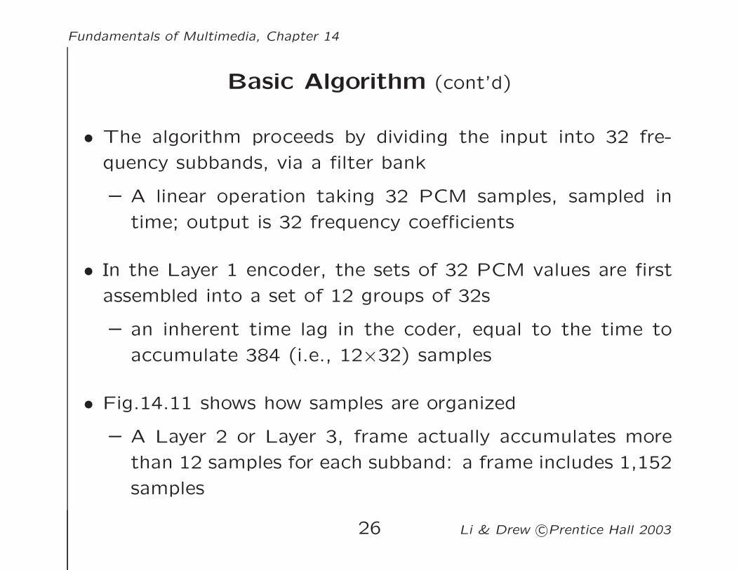
• Fig.14.11 shows how samples are organized
– A Layer 2 or Layer 3, frame actually accumulates more
than 12 samples for each subband: a frame includes 1,152
samples
26 Li & Drew c©Prentice Hall 2003
Fundamentals of Multimedia, Chapter 14
12samples
Each subband filter produces 1 sample outfor every 32 samples in
Audio (PCM)samples In
Subband filter 0
Subband filter 1
Subband filter 2
Subband filter 31Layer 1Frame
Layer 2 and Layer 3Frame
12samples
12samples
12samples
12samples
12samples
12samples
12samples
12samples
12samples
12samples
12samples
. . . . . .
. . .
. . .
Fig. 14.11: MPEG Audio Frame Sizes
27 Li & Drew c©Prentice Hall 2003
Fundamentals of Multimedia, Chapter 14
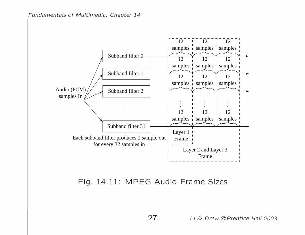
Bit Allocation Algorithm
• Aim: ensure that all of the quantization noise is below the
masking thresholds
• One common scheme:
– For each subband, the psychoacoustic model calculates the Signal-to-Mask Ratio (SMR)in dB
– Then the “Mask-to-Noise Ratio” (MNR) is defined as the difference(as shown in Fig.14.12):
MNRdB ≡ SNRdB − SMRdB (14.6)
– The lowest MNR is determined, and the number of code-bits allocatedto this subband is incremented
– Then a new estimate of the SNR is made, and the process iteratesuntil there are no more bits to allocate
28 Li & Drew c©Prentice Hall 2003

Fundamentals of Multimedia, Chapter 14
Sound pressurelevel (db) Masker
Minimummasking threshold
Neighboringband
Critical band Neighboringband
Bits allocatedto critical band
Frequency
m−1m+1m
SN
R SM
RM
NR
Fig. 14.12: MNR and SMR. A qualitative view of SNR, SMR and
MNR are shown, with one dominate masker and m bits allocated
to a particular critical band.
29 Li & Drew c©Prentice Hall 2003
Fundamentals of Multimedia, Chapter 14
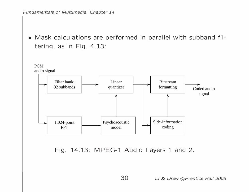
• Mask calculations are performed in parallel with subband fil-
tering, as in Fig. 4.13:
PCMaudio signal
Linearquantizer
Bitstreamformatting
Filter bank:32 subbands
1,024-pointFFT
Psychoacousticmodel
Coded audiosignal
Side-informationcoding
Fig. 14.13: MPEG-1 Audio Layers 1 and 2.
30 Li & Drew c©Prentice Hall 2003
Fundamentals of Multimedia, Chapter 14
Layer 2 of MPEG-1 Audio
• Main difference:
– Three groups of 12 samples are encoded in each frame andtemporal masking is brought into play, as well as frequencymasking
– Bit allocation is applied to window lengths of 36 samplesinstead of 12
– The resolution of the quantizers is increased from 15 bitsto 16
• Advantage:
– a single scaling factor can be used for all three groups
31 Li & Drew c©Prentice Hall 2003
Fundamentals of Multimedia, Chapter 14
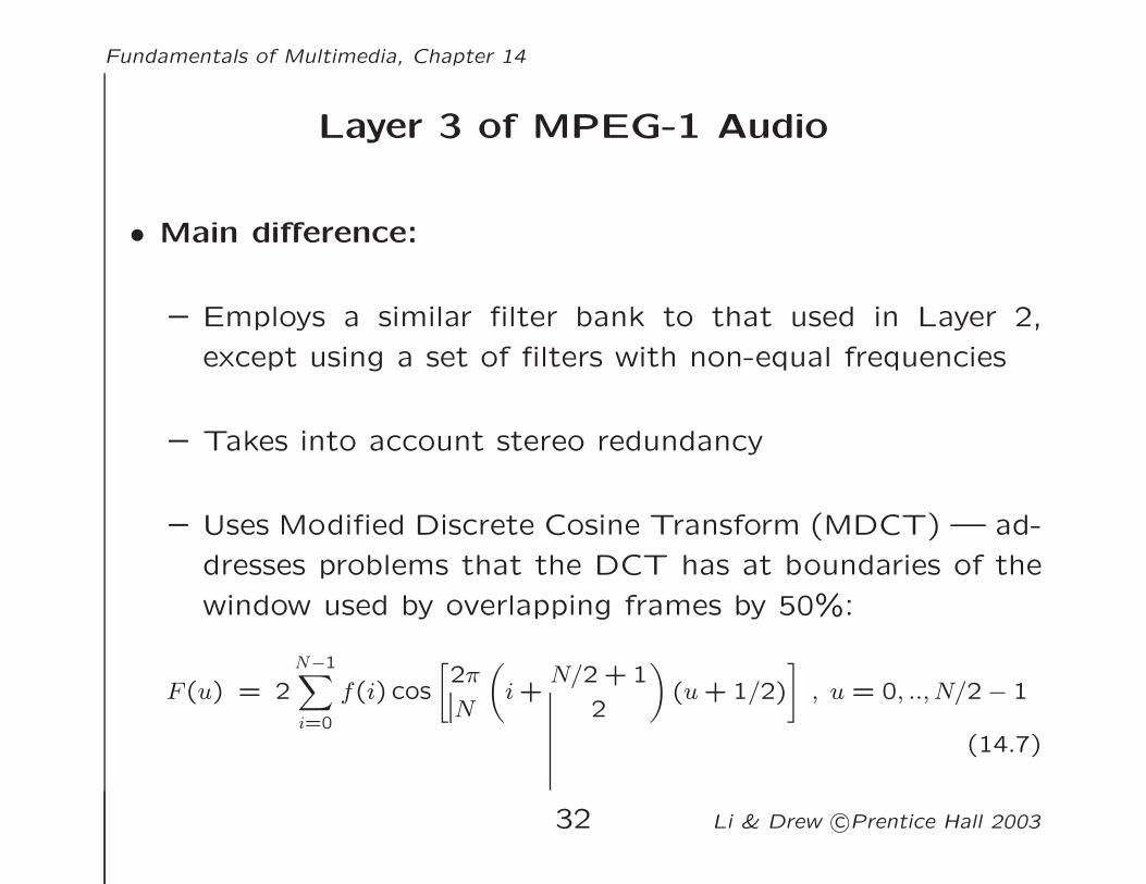
Layer 3 of MPEG-1 Audio
• Main difference:
– Employs a similar filter bank to that used in Layer 2,
except using a set of filters with non-equal frequencies
– Takes into account stereo redundancy
– Uses Modified Discrete Cosine Transform (MDCT) — ad-
dresses problems that the DCT has at boundaries of the
window used by overlapping frames by 50%:
F (u) = 2N−1∑i=0
f(i) cos
[2π
N
(i +
N/2 + 1
2
)(u + 1/2)
], u = 0, .., N/2− 1
(14.7)
32 Li & Drew c©Prentice Hall 2003
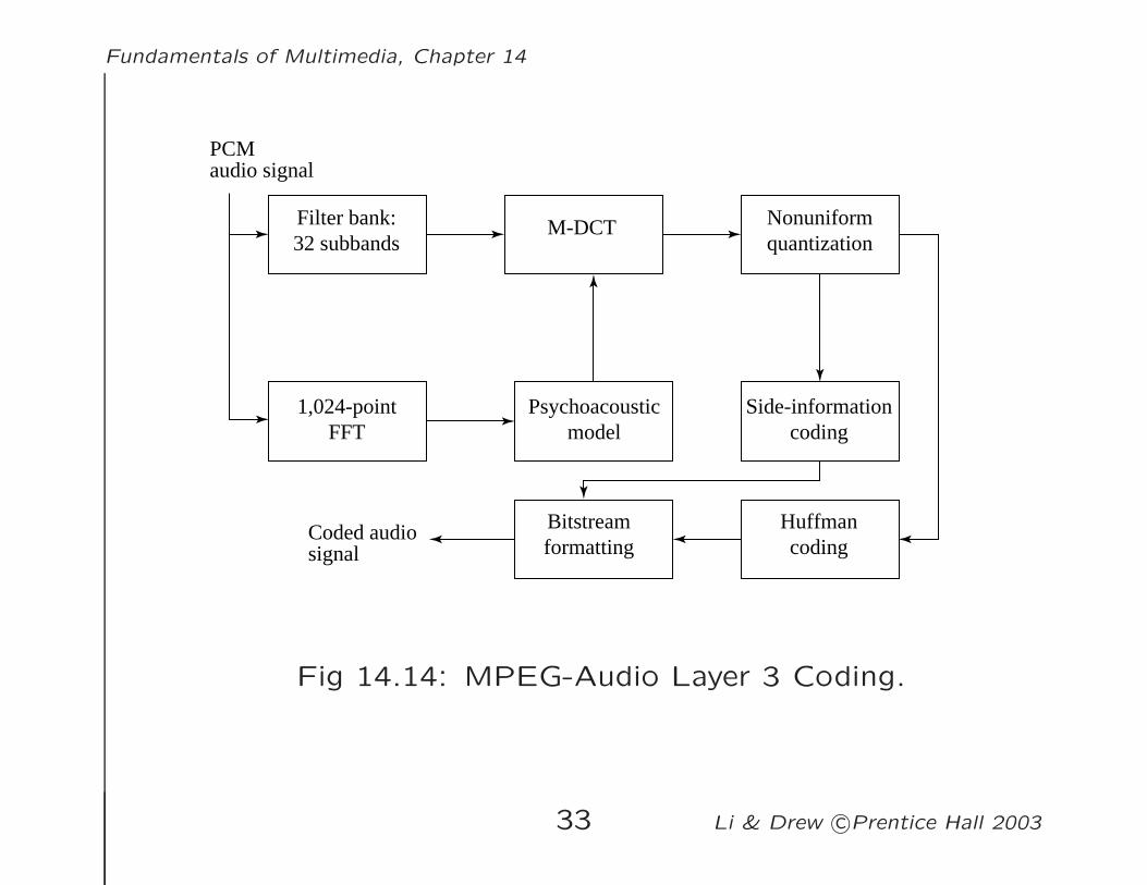
Fundamentals of Multimedia, Chapter 14
PCMaudio signal
Filter bank:32 subbands
1,024-pointFFT
Psychoacousticmodel
M-DCT Nonuniformquantization
Bitstreamformatting
Huffmancoding
Side-informationcoding
Coded audiosignal
Fig 14.14: MPEG-Audio Layer 3 Coding.
33 Li & Drew c©Prentice Hall 2003
Fundamentals of Multimedia, Chapter 14
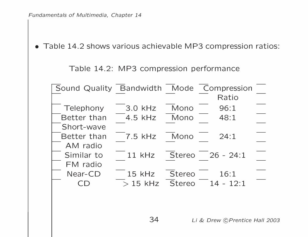
• Table 14.2 shows various achievable MP3 compression ratios:
Table 14.2: MP3 compression performance
Sound Quality Bandwidth Mode CompressionRatio
Telephony 3.0 kHz Mono 96:1Better than 4.5 kHz Mono 48:1Short-waveBetter than 7.5 kHz Mono 24:1AM radioSimilar to 11 kHz Stereo 26 - 24:1FM radioNear-CD 15 kHz Stereo 16:1
CD > 15 kHz Stereo 14 - 12:1
34 Li & Drew c©Prentice Hall 2003
Fundamentals of Multimedia, Chapter 14
MPEG-2 AAC (Advanced Audio Coding)
• The standard vehicle for DVDs:
– Audio coding technology for the DVD-Audio Recordable
(DVD-AR) format, also adopted by XM Radio
• Aimed at transparent sound reproduction for theaters
– Can deliver this at 320 kbps for five channels so that
sound can be played from 5 different directions: Left,
Right, Center, Left-Surround, and Right-Surround
• Also capable of delivering high-quality stereo sound at bit-
rates below 128 kbps
35 Li & Drew c©Prentice Hall 2003

Fundamentals of Multimedia, Chapter 14
MPEG-2 AAC (cont’d)
• Support up to 48 channels, sampling rates between 8 kHz
and 96 kHz, and bit-rates up to 576 kbps per channel
• Like MPEG-1, MPEG-2, supports three different “profiles”,
but with a different purpose:
– Main profile
– Low Complexity(LC) profile
– Scalable Sampling Rate (SSR) profile
36 Li & Drew c©Prentice Hall 2003
Fundamentals of Multimedia, Chapter 14
MPEG-4 Audio
• Integrates several different audio components into one stan-
dard: speech compression, perceptually based coders, text-
to-speech, and MIDI
• MPEG-4 AAC (Advanced Audio Coding), is similar to the
MPEG-2 AAC standard, with some minor changes
• Perceptual Coders
– Incorporate a Perceptual Noise Substitution module
– Include a Bit-Sliced Arithmetic Coding (BSAC) module
– Also include a second perceptual audio coder, a vector-
quantization method entitled TwinVQ
37 Li & Drew c©Prentice Hall 2003
Fundamentals of Multimedia, Chapter 14
MPEG-4 Audio (Cont’d)
• Structured Coders
– Takes “Synthetic/Natural Hybrid Coding” (SNHC) in or-
der to have very low bit-rate delivery an option
– Objective: integrate both “natural” multimedia sequences,
both video and audio, with those arising synthetically –
“structured” audio
– Takes a “toolbox” approach and allows specification of
many such models.
– E.g., Text-To-Speech (TTS) is an ultra-low bit-rate method,
and actually works, provided one need not care what the
speaker actually sounds like
38 Li & Drew c©Prentice Hall 2003
Fundamentals of Multimedia, Chapter 14
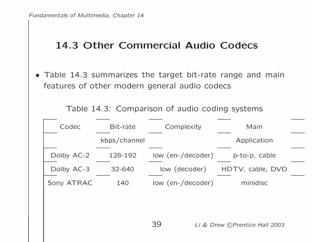
14.3 Other Commercial Audio Codecs
• Table 14.3 summarizes the target bit-rate range and main
features of other modern general audio codecs
Table 14.3: Comparison of audio coding systems
Codec Bit-rate Complexity Main
kbps/channel Application
Dolby AC-2 128-192 low (en-/decoder) p-to-p, cable
Dolby AC-3 32-640 low (decoder) HDTV, cable, DVD
Sony ATRAC 140 low (en-/decoder) minidisc
39 Li & Drew c©Prentice Hall 2003
Fundamentals of Multimedia, Chapter 14
14.4 The Future: MPEG-7 and MPEG-21
• Difference from current standards:
– MPEG-4 is aimed at compression using objects.
– MPEG-7 is mainly aimed at “search”: How can we find
objects, assuming that multimedia is indeed coded in terms
of objects
40 Li & Drew c©Prentice Hall 2003
Fundamentals of Multimedia, Chapter 14
– MPEG-7: A means of standardizing meta-data for au-
diovisual multimedia sequences – meant to represent in-
formation about multimedia information
In terms of audio: facilitate the representation and search
for sound content. Example application supported by
MPEG-7: automatic speech recognition (ASR).
– MPEG-21: Ongoing effort, aimed at driving a standard-
ization effort for a Multimedia Framework from a con-
sumer’s perspective, particularly interoperability
In terms of audio: support of this goal, using audio.
41 Li & Drew c©Prentice Hall 2003
Fundamentals of Multimedia, Chapter 14
14.5 Further Exploration−→ Link to Further Exploration for Chapter 14.
In Chapter 14 the “Further Exploration” section of the text web-
site, a number of useful links are given:
• Excellent collections of MPEG Audio and MP3 links.
• The “official” MPEG Audio FAQ
• MPEG-4 Audio implements “Tools for Large Step Scala-
bility”, An excellent reference is given by the Fraunhofer-
Gesellschaft research institute, “MPEG 4 Audio Scalable Pro-
file”.
42 Li & Drew c©Prentice Hall 2003


![EfficientBit AllocationAlgorithmFor MPEG-4 Audio · as MPEG-1/2/4 audio coding standards and Dolby AC-3 [1]. The MPEG-4 Advanced Audio Coding (AAC) is one ofthe mostrecent-generation](https://static.fdocuments.net/doc/165x107/5b3b16727f8b9a26728c2604/efficientbit-allocationalgorithmfor-mpeg-4-audio-as-mpeg-124-audio-coding.jpg)