Chapter 12More About Regression

Let’s look at the Warm-Up first to remind ourselves what we did with regression!

Remember FODS!

Section 12.1Inference for Linear RegressionLeast-Squares Regression fits a

straight line of the form to data to predict a response variable y from the explanatory variable x.

Inference in this setting uses the sample regression line to estimate or test a claim about the population (true) regression line.

Confidence intervals and significance tests about the slope of the population regression line are based on the sampling distribution of b, the slope of the sample regression line.

Conditions - LINER Linear – the actual relationship between x

and y is linear. For any fixed value of x, the mean response falls on the population (true) regression line – graph scatterplot

Independent – individual observations are independent

Normal – for any fixed value of x, the response y varies according to a Normal distribution – you will be graphing the Normal probability plot of the residuals here.

Equal Variance – the standard deviation of y (call it ) is the same for all values of x – graph residual plot

Random – the data are produced from a well-designed random sample or a randomized experiment.

How it works…The slope b and intercept a of the

least-squares regression line estimate the slope and the intercept of the population (true) regression line.

To estimate use the standard deviation of s of the residuals.

Confidence IntervalsConfidence intervals and significance

tests for the slope of the population regression line are based on a t distribution with n-2 degrees of freedom.

n-2 because we have two lists – we need to allow another degree of freedom for the extra variable…

The t interval for the slope has the form

The standard error of the slope is

Let’s look at SE…

On the AP formula sheet:

Hypothesis TestsTo test the null hypothesis, carry

out a t test for the slope.Use (The most common null

hypothesis is , which says that there is no linear relationship between x and y in the population.

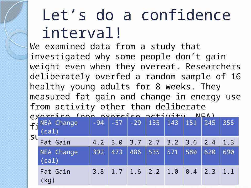
Let’s do a confidence interval!

We examined data from a study that investigated why some people don’t gain weight even when they overeat. Researchers deliberately overfed a random sample of 16 healthy young adults for 8 weeks. They measured fat gain and change in energy use from activity other than deliberate exercise (non-exercise activity, NEA) – fidgeting, daily living, etc – for each subject. Here are the results:

NEA Change (cal)

-94 -57 -29 135 143 151 245 355

Fat Gain (kg) 4.2 3.0 3.7 2.7 3.2 3.6 2.4 1.3

NEA Change (cal)

392 473 486 535 571 580 620 690

Fat Gain (kg) 3.8 1.7 1.6 2.2 1.0 0.4 2.3 1.1

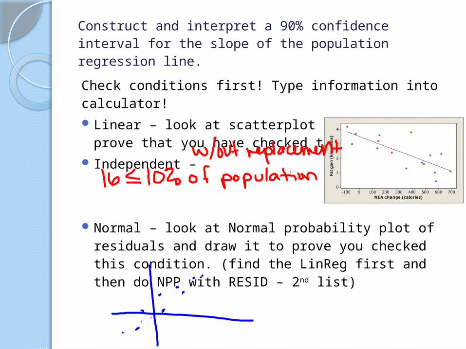
Construct and interpret a 90% confidence interval for the slope of the population regression line.

Check conditions first! Type information into calculator!Linear – look at scatterplot and draw it to

prove that you have checked this condition. Independent –

Normal – look at Normal probability plot of residuals and draw it to prove you checked this condition. (find the LinReg first and then do NPP with RESID – 2nd list)

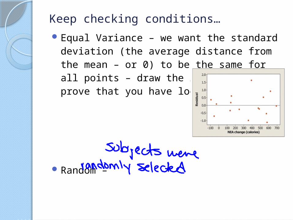
Keep checking conditions…Equal Variance – we want the standard

deviation (the average distance from the mean – or 0) to be the same for all points – draw the residual plot to prove that you have looked at it.

Random –

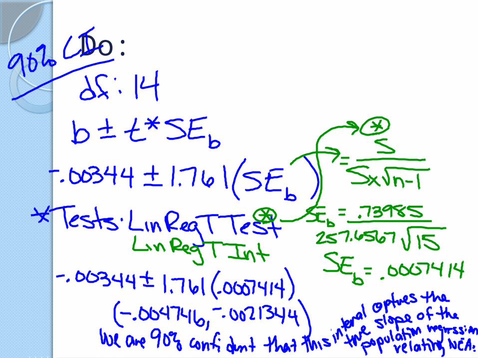
Do:

A Significance Test…Infants who cry easily may be more easily stimulated than others. This may be a sign of higher IQ. Researchers explored the relationship between crying infants 4 to 10 days old and their later IQ scores. The researchers flicked the infants with a rubber band and recorded the crying. They measured its intensity by the number of peaks in the most active 20 seconds. The table below contains data from a random sample of 38 infants.

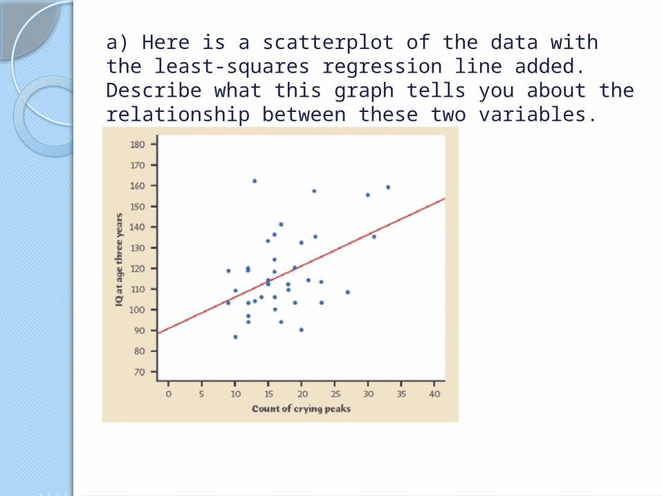
a) Here is a scatterplot of the data with the least-squares regression line added. Describe what this graph tells you about the relationship between these two variables.

b) Using the min-tab output, what is the equation of the least-squares regression line?

c) Interpret slope and y-intercept of the regression line in context

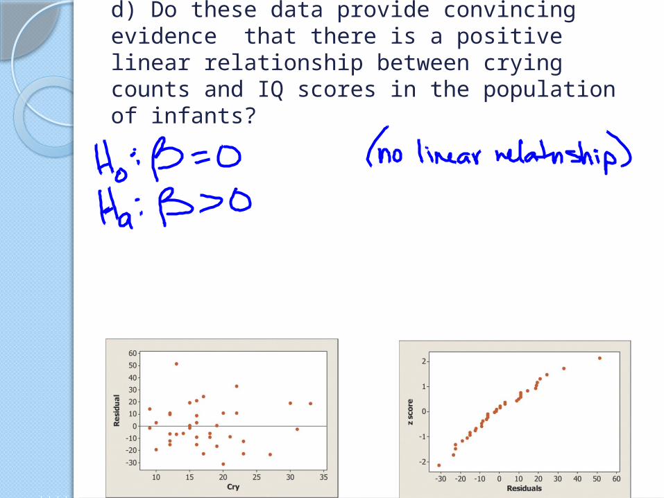
d) Do these data provide convincing evidence that there is a positive linear relationship between crying counts and IQ scores in the population of infants?

HomeworkPg 759 (6, 8, 13-15, 18-26)