Stormwater Drainage Design and Stormwater Quality Control ...

ODOT ROADWAY DRAINAGE MANUAL
November 2014
Chapter 10
STORMWATER DRAINAGE

ODOT Roadway Drainage Manual November 2014
Stormwater Drainage 10-i
Chapter 10 STORMWATER DRAINAGE
Table of Contents
Section Page 10.1 INTRODUCTION ..................................................................................................... 10.1-1
10.1.1 Overview ................................................................................................ 10.1-1 10.1.2 Inadequate Drainage ............................................................................. 10.1-1 10.1.3 General Design Guidelines .................................................................... 10.1-2
10.2 SYMBOLS, DEFINITIONS AND UNITS .................................................................. 10.2-3 10.3 DEFINITIONS OF TERMS ...................................................................................... 10.3-1 10.4 ODOT POLICY ........................................................................................................ 10.4-1
10.4.1 Roadside Channels and Ditches ........................................................... 10.4-1 10.4.2 Hydrology .............................................................................................. 10.4-1 10.4.3 Water Spread ........................................................................................ 10.4-1 10.4.4 Inlet Types ............................................................................................. 10.4-2 10.4.5 Manholes ............................................................................................... 10.4-2 10.4.6 Storm Drains .......................................................................................... 10.4-3 10.4.7 Property Development Drainage Policy ................................................. 10.4-3 10.4.8 Flood Hazard ......................................................................................... 10.4-3 10.4.9 Detention Storage .................................................................................. 10.4-4
10.5 DESIGN CRITERIA ................................................................................................. 10.5-1
10.5.1 Design Flood Frequency and Spread .................................................... 10.5-1 10.5.2 Risk Assessment ................................................................................... 10.5-2 10.5.3 Review Flood Frequency ....................................................................... 10.5-2 10.5.4 Sheet Flow Across Pavement ............................................................... 10.5-2
10.6 GENERAL CONSIDERATIONS .............................................................................. 10.6-1
10.6.1 Hydroplaning ......................................................................................... 10.6-1 10.6.2 Urban Water Quality Practices .............................................................. 10.6-1 10.6.3 Inverted Siphons .................................................................................... 10.6-2 10.6.4 Underdrains ........................................................................................... 10.6-2
10.7 GENERAL DESIGN APPROACH ........................................................................... 10.7-1
10.7.1 Design Process ..................................................................................... 10.7-1 10.7.2 Location and Size Guidelines ................................................................ 10.7-1 10.7.3 Outfall Guidelines .................................................................................. 10.7-1
10.8 HYDROLOGY ......................................................................................................... 10.8-1

ODOT Roadway Drainage Manual November 2014
10-ii Stormwater Drainage
Table of Contents (Continued)
Section Page
10.8.1 Introduction ............................................................................................ 10.8-1 10.8.2 Design Frequency ................................................................................. 10.8-1 10.8.3 Review Frequency ................................................................................. 10.8-1 10.8.4 Rational Method .................................................................................... 10.8-1 10.8.5 Time of Concentration ........................................................................... 10.8-2
10.8.5.1 Introduction ....................................................................... 10.8-2 10.8.5.2 Inlet Spacing ..................................................................... 10.8-2 10.8.5.3 Pipe Sizing ........................................................................ 10.8-2 10.8.5.4 Summary ........................................................................... 10.8-2
10.9 ROADWAY GEOMETRICS .................................................................................... 10.9-1
10.9.1 Introduction ............................................................................................ 10.9-1 10.9.2 Roadway Cross Section ........................................................................ 10.9-1
10.9.2.1 Width ................................................................................. 10.9-1 10.9.2.2 Cross Slope ...................................................................... 10.9-1
10.9.3 Vertical Alignment .................................................................................. 10.9-2
10.9.3.1 Longitudinal Slope ............................................................ 10.9-2 10.9.3.2 Vertical Curves .................................................................. 10.9-2
10.9.4 Curb and Gutter ..................................................................................... 10.9-2 10.9.5 Medians ................................................................................................. 10.9-3
10.9.5.1 Flush Medians ................................................................... 10.9-3 10.9.5.2 Curbed Medians ................................................................ 10.9-3 10.9.5.3 Median Barriers ................................................................. 10.9-3
10.10 GUTTER FLOW CALCULATIONS.......................................................................... 10.10-1
10.10.1 Introduction ............................................................................................ 10.10-1 10.10.2 Capacity Relationship ............................................................................ 10.10-1 10.10.3 Uniform Cross Slope Procedure ............................................................ 10.10-2 10.10.4 Composite Gutter Section Procedure .................................................... 10.10-3
10.11 INLET TYPES ......................................................................................................... 10.11-1
10.11.1 General .................................................................................................. 10.11-1 10.11.2 Types ..................................................................................................... 10.11-1
10.11.2.1 Grate Inlets ....................................................................... 10.11-2 10.11.2.2 Curb-Opening Inlets .......................................................... 10.11-2 10.11.2.3 Combination Inlets ............................................................ 10.11-2 10.11.2.4 Slotted Drain Inlets ............................................................ 10.11-2

ODOT Roadway Drainage Manual November 2014
Stormwater Drainage 10-iii
Table of Contents (Continued)
Section Page
10.11.3 Drop Inlets ............................................................................................. 10.11-2 10.12 INLET LOCATION, SPACING AND CAPACITY ..................................................... 10.12-1
10.12.1 Location ................................................................................................. 10.12-1 10.12.2 Spacing Process .................................................................................... 10.12-1 10.12.3 Grate Inlets on Grade ............................................................................ 10.12-2 10.12.4 Grate Inlets in Sag ................................................................................. 10.12-6 10.12.5 Curb Opening Inlets on Grade ............................................................... 10.12-9 10.12.6 Curb-Opening Inlets in Sag ................................................................... 10.12-11 10.12.7 Combination Inlet on Grade ................................................................... 10.12-14 10.12.8 Combination Inlet in Sag ....................................................................... 10.12-14 10.12.9 Flanking Inlets ....................................................................................... 10.12-14 10.12.10 Inlet Spacing Computations ................................................................... 10.12-17
10.13 ODOT STORM DRAIN PRACTICE......................................................................... 10.13-1
10.13.1 Pipe Material .......................................................................................... 10.13-1
10.13.1.1 Minimum Pipe Size ........................................................... 10.13-1 10.13.1.2 Pipe Material ..................................................................... 10.13-1 10.13.1.3 Minimum Pipe Cover and Clearance ................................ 10.13-1 10.13.1.4 Joint Seals ........................................................................ 10.13-1 10.13.1.5 Pipe-to-Inlet Connections .................................................. 10.13-2 10.13.1.6 Pipe Gradients .................................................................. 10.13-2
10.13.2 Hydraulic Analysis ................................................................................. 10.13-3
10.13.2.1 Pipe Flow .......................................................................... 10.13-3 10.13.2.2 Minimum Velocity .............................................................. 10.13-3 10.13.2.3 Maximum Velocity ............................................................. 10.13-3 10.13.2.4 Gradients .......................................................................... 10.13-3
10.13.3 HEC-22 Design Method ......................................................................... 10.13-3 10.13.4 Minimum Grades ................................................................................... 10.13-4 10.13.5 Curved Alignment .................................................................................. 10.13-5 10.13.6 Manholes ............................................................................................... 10.13-5
10.13.6.1 Location ............................................................................ 10.13-5 10.13.6.2 Spacing ............................................................................. 10.13-6 10.13.6.3 Sizing ................................................................................ 10.13-6 10.13.6.4 Shaping Inside of Manhole ............................................... 10.13-6
10.13.7 Sag Point ............................................................................................... 10.13-6

ODOT Roadway Drainage Manual November 2014
10-iv Stormwater Drainage
Table of Contents (Continued)
Section Page 10.14 INITIAL SIZE OF PIPE ............................................................................................ 10.14-1
10.14.1 Introduction ............................................................................................ 10.14-1 10.14.2 Design Procedures ................................................................................ 10.14-1 10.14.3 Storm Sewer Design Procedure ............................................................ 10.14-2
10.14.3.1 How to Fill the columns of Figure 10.14-A ........................ 10.14-4
10.15 HYDRAULIC GRADE LINE CALCULATION........................................................... 10.15-1
10.15.1 Introduction ............................................................................................ 10.15-1 10.15.2 ODOT Practice (HGL) ........................................................................... 10.15-2 10.15.3 Tailwater ................................................................................................ 10.15-2 10.15.4 Energy Losses ....................................................................................... 10.15-3
10.15.4.1 Exit Losses ........................................................................ 10.15-3 10.15.4.2 Pipe Friction Losses .......................................................... 10.15-3 10.15.4.3 Bend Losses ..................................................................... 10.15-4 10.15.4.4 Manhole/Inlet Losses Inlet ................................................ 10.15-4 10.15.4.5 Manhole Loss Estimate ..................................................... 10.15-5 10.15.4.6 Manhole Losses (HEC-22 Method) ................................... 10.15-5 10.15.4.7 ODOT Manhole Loss Method ........................................... 10.15-6
10.15.5 Hydraulic Grade Line Design Procedure ............................................... 10.15-10
10.16 ODOT DESIGN EXAMPLE ..................................................................................... 10.16-1
10.16.1 Layout and Data .................................................................................... 10.16-1 10.16.2 Initial Size .............................................................................................. 10.16-5 10.16.3 Hydraulic Grade Line ............................................................................. 10.16-8 10.16.4 Manhole MH5 ........................................................................................ 10.16-9 10.16.5 Manhole MH4 ........................................................................................ 10.16-10 10.16.6 Manhole MH3 ........................................................................................ 10.16-16 10.16.7 Manhole MH2 ........................................................................................ 10.16-18 10.16.8 Manhole MH1 ........................................................................................ 10.16-21 10.16.9 Inlet I2 .................................................................................................... 10.16-23 10.16.10 Inlet I1 .................................................................................................... 10.16-25
10.17 REFERENCES ........................................................................................................ 10.17-1
ODOT Roadway Drainage Manual November 2014
List of Figures 10-v
List of Figures
Figure Page Figure 10.2-A — SYMBOLS (Definitions and Units) ....................................................... 10.2-3 Figure 10.4-A — MANHOLE SPACING .......................................................................... 10.4-3 Figure 10.5-A — ODOT DESIGN FREQUENCY AND SPREAD GUIDELINES
FOR STORM DRAINS ......................................................................... 10.5-1 Figure 10.10-A — TYPICAL CURB AND GUTTER SECTIONS ....................................... 10.10-1 Figure 10.10-B — MANNING’S n FOR GUTTERS ........................................................... 10.10-2 Figure 10.11-A — INLET TYPES ...................................................................................... 10.11-1 Figure 10.12-A — SPLASHOVER VELOCITY EQUATIONS ............................................ 10.12-3 Figure 10.12-B — GRATE INLET FRONTAL-FLOW INTERCEPTION EFFICIENCY ...... 10.12-5 Figure 10.12-C — CURB OPENING INLETS .................................................................... 10.12-12 Figure 10.12-D — FLANKING INLETS AT SAG POINT ................................................... 10.12-15 Figure 10.12-E — INLET SPACING COMPUTATION SHEET ......................................... 10.12-20 Figure 10.13-A — MINIMUM SLOPES NECESSARY TO ENSURE 3 fps IN
STORM DRAINS FLOWING FULL (Equation 10.13(4)) ...................... 10.13-5 Figure 10.13-B — EFFICIENT MANHOLE SHAPING ....................................................... 10.13-7 Figure 10.14-A — STORM SEWER COMPUTATION FORM ........................................... 10.14-3 Figure 10.14-B — NOMOGRAPH FOR FLOW IN ROUND PIPE –
MANNING’S FORMULA ...................................................................... 10.14-6 Figure 10.15-A — HYDRAULIC AND ENERGY GRADE LINE ILLUSTRATION .............. 10.15-1 Figure 10.15-B — KM BASED ON STRUCTURE CONFIGURATION ............................... 10.15-5 Figure 10.15-C — DEFINITION SKETCH FOR HEC-22 (2009) MANHOLE
LOSS METHOD ................................................................................... 10.15-6 Figure 10.15-D — BEND LOSS – OPEN CHANNEL FLOW DESIGN .............................. 10.15-9 Figure 10.15-E — SEWER BEND LOSS COEFFICIENT, K ............................................. 10.15-13 Figure 10.15-F — RECTANGULAR INLET WITH THROUGH PIPELINE AND
GRATE FLOW ..................................................................................... 10.15-14 Figure 10.15-G — RECTANGULAR INLET WITH IN-LINE OPPOSED LATERAL
PIPES EACH AT 90° TO OUTFALL (WITH OR WITHOUT GRATE FLOW) .................................................................................... 10.15-15
Figure 10.15-H — FLOW STRAIGHT THROUGH ANY JUNCTION ................................. 10.15-16 Figure 10.15-I — SQUARE OR ROUND MANHOLE AT 90° DEFLECTION OR ON
THROUGH PIPELINE AT JUNCTION OF 90° LATERAL PIPE (LATERAL COEFFICIENT) .................................................................. 10.15-17
Figure 10.15-J — SQUARE OR ROUND MANHOLE ON THROUGH PIPELINE AT JUNCTION OF A 90° LATERAL PIPE (IN-LINE PIPE COEFFICIENT) ........................................................................... 10.15-18
Figure 10.15-K — SQUARE OR ROUND MANHOLE ON THROUGH PIPELINE AT JUNCTION OF 90° LATERAL PIPE (for conditions outside range of Figures 10.15-I and 10.15-J) .................................................. 10.15-19
Figure 10.15-L — RECTANGULAR INLET WITH GRATE FLOW ONLY ......................... 10.15-20
ODOT Roadway Drainage Manual November 2014
10-vi Stormwater Drainage
List of Figures (Continued)
Figure Page Figure 10.15-M — HYDRAULIC GRADE LINE COMPUTATION FORM .......................... 10.15-21 Figure 10.16-A — STORM SEWER SYSTEM LAYOUT ................................................... 10.16-3 Figure 10.16-B — GROUND PROFILE – LINE A ............................................................. 10.16-4 Figure 10.16-C — PRELIMINARY STORM SEWER DESIGN .......................................... 10.16-5 Figure 10.16-D — STORM SEWER PROFILE – LINE A .................................................. 10.16-6 Figure 10.16-E — HYDRAULIC GRADE LINE PROFILE – LINE A .................................. 10.16-7 Figure 10.16-F — PRELIMINARY STORM SEWER DESIGN .......................................... 10.16-8 Figure 10.16-G — RELATIVE V, A, Q IN A CIRCULAR PIPE FOR ANY DEPTH
OF FLOW, WITH CONSTANT “N” ....................................................... 10.16-13

ODOT Roadway Drainage Manual November 2014
Stormwater Drainage 10.1-1
Chapter 10 STORMWATER DRAINAGE
10.1 INTRODUCTION
10.1.1 Overview
This chapter provides policy guidance on all elements of storm drainage design: system planning, pavement drainage, gutter flow calculations, inlet spacing, pipe sizing and hydraulics grade line calculations, maintenance and control of runoff from future development, which are based on the AASHTO Drainage Manual (1), Chapter 13 “Storm Drain Systems.” This chapter provides guidance on all elements of storm drainage design:
• design policy (Section 10.4); • criteria (Section 10.5); • general considerations (Section 10.6); • general design approach (Section 10.7); • hydrology (Section 10.8); • roadway geometrics (Section 10.9); • gutter flow calculations (Section 10.10); • inlet types (Section 10.11); • inlet location, spacing and capacity (Section 10.12); • ODOT Practice (Section 10.13); • initial sizing of pipe (Section 10.14); • hydraulic grade line calculation (Section 10.15); and • ODOT design example (Section 10.16).
The design of a drainage system should address the needs of the traveling public and those of the local community through which it passes. The drainage system for a roadway traversing an urban area is more complex than for roadways traversing sparsely settled rural areas. This is due to:
• the wide roadway sections, flat grades (both in longitudinal and transverse directions), shallow water courses and absence of side channels;
• the more costly property damage that may occur from ponding of water or from flow of water through built-up areas; and
• the roadway section must carry traffic but also act as a channel to convey the water to a disposal point. Unless proper precautions are taken, this flow of water along the roadway may interfere with or possibly halt the passage of highway traffic.
10.1.2 Inadequate Drainage
The most serious effects of an inadequate storm drainage system are:
ODOT Roadway Drainage Manual November 2014
10.1-2 Stormwater Drainage
• damage to adjacent property, resulting from water overflowing the roadway curbs and entering such property;
• risk and delay to traffic caused by excessive ponding in sags or excessive spread along the roadway; and
• weakening of the base and subgrade due to saturation from frequent ponding of long duration.
10.1.3 General Design Guidelines
A storm drain is defined as that portion of the storm drainage system that receives runoff from inlets and conveys the runoff to some point where it is then discharged into a channel, water body or piped system:
• A storm drain may be a closed-conduit, open-conduit or some combination of the two.
• System may be designed with consideration for future development, if appropriate.
• A higher design frequency (or return interval) should be used for storm drain systems located in a major sag vertical curve to decrease the depth of ponding on the roadway and bridges and potential inundation of adjacent property.
• Where feasible, the storm drains should be designed to avoid existing utilities.
• Attention should be provided to the storm drain outfalls to ensure that the potential for erosion is minimized.
• Drainage system design should be coordinated with the proposed staging of large construction projects to maintain an outlet throughout the construction project.
This chapter discusses design procedures for storm drainage design and analysis, which are based on FHWA HEC-22 (2) . For additional guidance, refer to the AASHTO Highway Drainage Guidelines (3), Chapter 9 “Storm Drain Systems.”
ODOT Roadway Drainage Manual November 2014
Stormwater Drainage 10.2-3
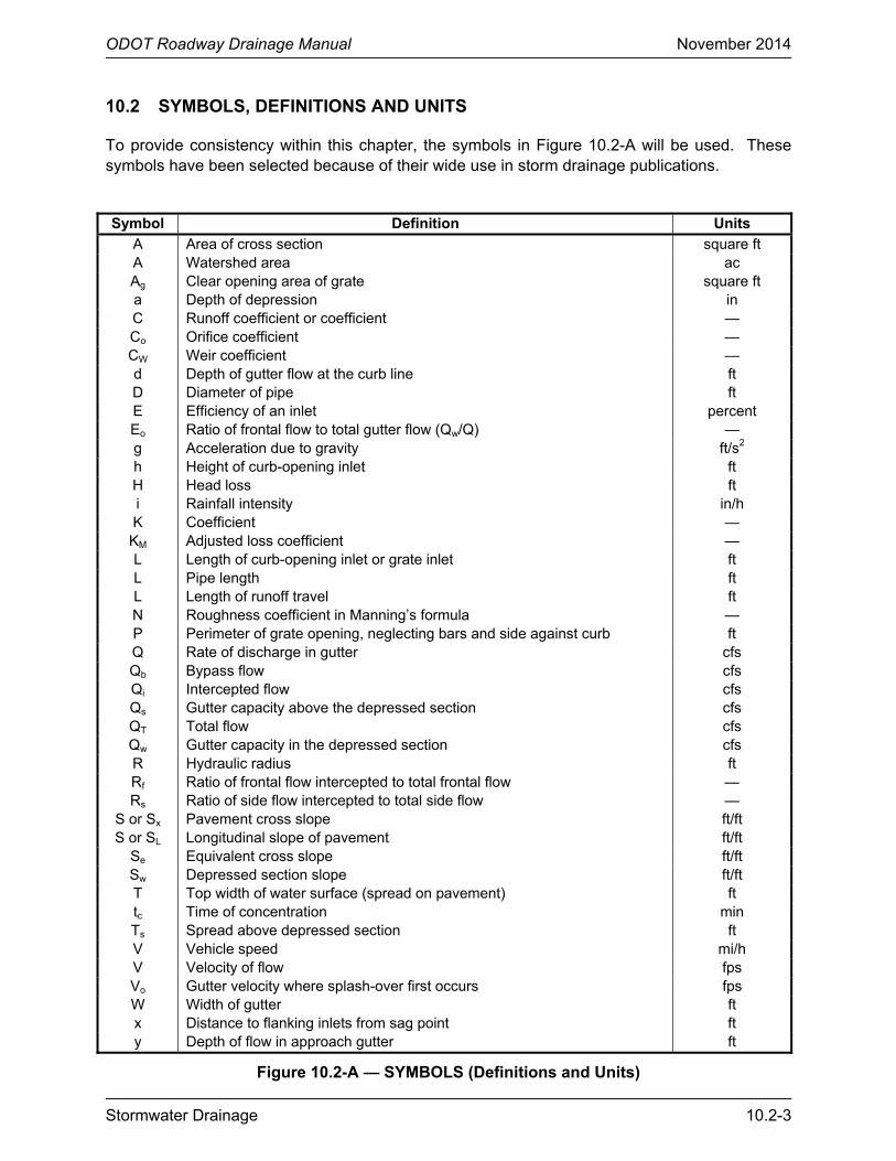
10.2 SYMBOLS, DEFINITIONS AND UNITS
To provide consistency within this chapter, the symbols in Figure 10.2-A will be used. These symbols have been selected because of their wide use in storm drainage publications.
Symbol Definition Units
A Area of cross section square ft A Watershed area ac Ag Clear opening area of grate square ft a Depth of depression in C Runoff coefficient or coefficient — Co Orifice coefficient — CW Weir coefficient — d Depth of gutter flow at the curb line ft D Diameter of pipe ft E Efficiency of an inlet percent Eo Ratio of frontal flow to total gutter flow (Qw/Q) — g Acceleration due to gravity ft/s2 h Height of curb-opening inlet ft H Head loss ft i Rainfall intensity in/h K Coefficient — KM Adjusted loss coefficient — L Length of curb-opening inlet or grate inlet ft L Pipe length ft L Length of runoff travel ft N Roughness coefficient in Manning’s formula — P Perimeter of grate opening, neglecting bars and side against curb ft Q Rate of discharge in gutter cfs Qb Bypass flow cfs Qi Intercepted flow cfs Qs Gutter capacity above the depressed section cfs QT Total flow cfs Qw Gutter capacity in the depressed section cfs R Hydraulic radius ft Rf Ratio of frontal flow intercepted to total frontal flow — Rs Ratio of side flow intercepted to total side flow —
S or Sx Pavement cross slope ft/ft S or SL Longitudinal slope of pavement ft/ft
Se Equivalent cross slope ft/ft Sw Depressed section slope ft/ft T Top width of water surface (spread on pavement) ft tc Time of concentration min Ts Spread above depressed section ft V Vehicle speed mi/h V Velocity of flow fps Vo Gutter velocity where splash-over first occurs fps W Width of gutter ft x Distance to flanking inlets from sag point ft y Depth of flow in approach gutter ft
Figure 10.2-A — SYMBOLS (Definitions and Units)

ODOT Roadway Drainage Manual November 2014
10.2-4 Stormwater Drainage

ODOT Roadway Drainage Manual November 2014
Stormwater Drainage 10.3-1
10.3 DEFINITIONS OF TERMS
The following definitions are important in storm drainage analysis and design. These definitions will be used throughout this chapter to address different aspects of storm drainage analysis:
1. Bypass. Carryover flow that bypasses an inlet on grade and is carried in the street or channel to the next inlet downgrade. Inlets can be designed to allow a certain amount of bypass for one design storm and larger or smaller amounts for other storms.
2. Combination Inlet. A drainage inlet usually composed of a curb-opening inlet and a grate inlet.
3. Crown. The crown, sometimes known as the soffit, is the top inside of a pipe.
4. Curb-Opening. A drainage inlet consisting of an opening in the roadway curb.
5. Drop Inlet. A vertical or inclined inlet (usually a box) which is used for dropping the water (on the surface, in a conduit or in a channel) to a lower level and dissipating its surplus energy. See AASHTO Glossary, (3).
6. Equivalent Cross Slope. An imaginary straight cross slope having conveyance capacity equal to that of the given compound cross slope.
7. Flanking Inlets. Inlets placed upstream and on either side of an inlet at the low point in a sag vertical curve. These inlets intercept debris as the slope decreases and act in relief of the inlet at the low point.
8. Frontal Flow. The portion of the flow that passes over the upstream side of a grate.
9. Grate Inlet. A drainage inlet composed of a grate in the roadway section or at the roadside in a low point, swale or channel.
10. Grate Perimeter. The sum of the lengths of all sides of a grate, except that any side adjacent to a curb is not considered a part of the perimeter in weir-flow computations.
11. Gutter. That portion of the roadway section adjacent to the curb used to convey stormwater runoff. A composite gutter section consists of the section immediately adjacent to the curb, which has a cross slope steeper than the adjacent pavement and the parking lane, shoulder or pavement at a cross slope of a lesser amount. A uniform gutter section has one constant cross slope.
12. Hydraulic Grade Line. A line joining the elevations to which the water would rise in successive piezometer tubes if the tubes were installed along a pipe run (a closed conduit). It is equal to the pressure head plus the elevation head. It is also equal to the energy grade line minus the velocity head. In an open conduit (stream, channel, river etc.), the hydraulic grade line is the water surface profile.
13. Inlet Efficiency. The ratio of flow intercepted by an inlet to total flow in the gutter.
14. Invert. The inside bottom of the pipe.
ODOT Roadway Drainage Manual November 2014
10.3-2 Stormwater Drainage
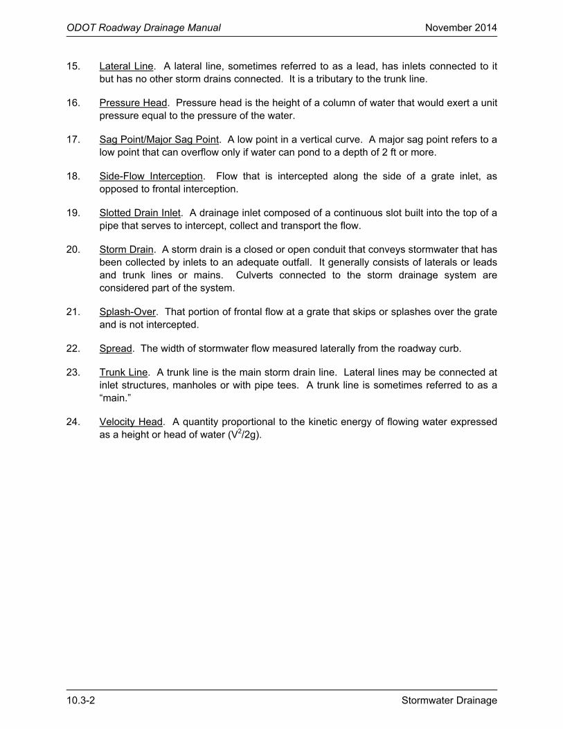
15. Lateral Line. A lateral line, sometimes referred to as a lead, has inlets connected to it but has no other storm drains connected. It is a tributary to the trunk line.
16. Pressure Head. Pressure head is the height of a column of water that would exert a unit pressure equal to the pressure of the water.
17. Sag Point/Major Sag Point. A low point in a vertical curve. A major sag point refers to a low point that can overflow only if water can pond to a depth of 2 ft or more.
18. Side-Flow Interception. Flow that is intercepted along the side of a grate inlet, as opposed to frontal interception.
19. Slotted Drain Inlet. A drainage inlet composed of a continuous slot built into the top of a pipe that serves to intercept, collect and transport the flow.
20. Storm Drain. A storm drain is a closed or open conduit that conveys stormwater that has been collected by inlets to an adequate outfall. It generally consists of laterals or leads and trunk lines or mains. Culverts connected to the storm drainage system are considered part of the system.
21. Splash-Over. That portion of frontal flow at a grate that skips or splashes over the grate and is not intercepted.
22. Spread. The width of stormwater flow measured laterally from the roadway curb.
23. Trunk Line. A trunk line is the main storm drain line. Lateral lines may be connected at inlet structures, manholes or with pipe tees. A trunk line is sometimes referred to as a “main.”
24. Velocity Head. A quantity proportional to the kinetic energy of flowing water expressed as a height or head of water (V2/2g).
ODOT Roadway Drainage Manual November 2014
Stormwater Drainage 10.4-1
10.4 ODOT POLICY
Highway storm drainage facilities collect stormwater runoff and convey it through the roadway right-of-way in a manner that adequately drains the roadway and minimizes the potential for flooding and erosion to properties adjacent to the right-of-way. Storm drainage facilities consist of curbs, gutters, storm drains, channels and culverts. The placement and hydraulics capacities of storm drainage facilities should be designed to consider the potential for damage to adjacent property and to secure a degree of risk of traffic interruption by flooding as is consistent with the importance of the road, the design traffic service requirements and available funds. Following is a summary of policies that should be followed for storm drain design and analysis.
10.4.1 Roadside Channels and Ditches
Large amounts of runoff should be intercepted before it reaches the highway in order to minimize the deposition of sediment or debris on the roadway and to reduce the amount of water which must be carried in the gutter section. Slope median areas and inside shoulders to a center depression to prevent runoff from the median area from running across the pavement. Surface channels should have adequate capacity for the design runoff and should be located and shaped in a manner that does not present a traffic hazard. Where permitted by the design velocities, channels should have a vegetative lining. Appropriate linings may be necessary where vegetation will not control erosion, see Chapter 8 “Channels.” Right-of-way restrictions/costs in urban areas often render impracticable the provision of roadside ditches.
10.4.2 Hydrology
The Rational Method is the most common method in use for the design of storm drains when the momentary peak-flow rate is desired, see Section 10.8. Its use should be limited to systems with drainage areas of 640 acres or less. A minimum time of concentration of 10 minutes is generally acceptable for well developed, flat slope urban areas. If the urban area is densely developed and steep, use 5 minutes. Drainage systems involving detention storage, pumping stations and large or complex storm systems require the development of a runoff hydrograph. The Rational Method and hydrograph methods are described in Chapter 7 “Hydrology.” The design frequency and spread criteria are discussed in Section 10.5.
ODOT does not use a hydrograph to compute peak discharge in storm drain design, except when detention storage is involved.
10.4.3 Water Spread
The top width of the open channel flow in the gutter is considered the spread. In general, the water spread should be limited to a specified width for the selected design frequency (see Section 10.5.1). For storms of greater magnitude, the spread can be allowed to use most of the pavement as an open channel. For multilane curb and gutter or guttered roadways with no parking, it is not practical to avoid travel lane flooding when longitudinal grades are flat (0.2% to 1%). The spread width may be adjusted if warranted by an assessment of the costs vs. risks. If the above spread requirement results in very close inlet spacing (i.e., 100 ft or less), then

ODOT Roadway Drainage Manual November 2014
10.4-2 Stormwater Drainage
alternative drainage interceptors could be considered. This may include allowing the spread to cover the outside lanes of a roadway with four lanes or more depending on the project conditions.
10.4.4 Inlet Types
The term “inlets” refers to all types of inlets (e.g., grate inlets, curb inlets, slotted inlets), see Section 10.11. Drainage inlets are sized and located to limit the spread of water on traffic lanes to tolerable widths for the design storm in accordance with the design criteria specified in Section 10.5. The width of water spread on the pavement at sags should not be substantially greater than the width of spread encountered on continuous grades.
Grate inlets and depression of curb opening inlets should be located outside the through traffic lanes to minimize the shifting of vehicles attempting to avoid them. All grate inlets should be bicycle safe where used on roadways that allow bicycle travel. Curb inlets are preferred to grate inlets at major sag locations because of their debris handling capabilities. When grate inlets are used at sag locations, assume that they are half plugged with debris and size accordingly.
In locations where significant ponding may occur (e.g., underpasses, sag vertical curves in depressed sections), recommended practice is to place flanking inlets on each side of the inlet at the low point in the sag.
10.4.5 Manholes
Manholes are used to provide entry to continuous underground storm drains for inspection and cleanout. Some state highway agencies use grate inlets in lieu of manholes when entry to the system can be provided at the grate inlet, so that the benefit of extra stormwater interception can be achieved with minimal additional cost. Also, a combination of inlet and manhole is sometimes used to reduce the storm sewer foot print and cost. Typical locations where manholes should be specified are:
• where two or more storm drains converge, • at intermediate points along tangent sections, • where pipe size changes, • where an abrupt change in alignment occurs, and • where an abrupt change of the grade occurs.
Manholes should not be located in traffic lanes; however, where it is impossible to avoid locating a manhole in a traffic lane, care should be taken to ensure that it is not in the normal vehicular wheel path. The spacing of manholes should be in accordance with Figure 10.4-A.

ODOT Roadway Drainage Manual November 2014
Stormwater Drainage 10.4-3
Size of Pipe (in) Maximum Distance (ft)
12 – 24 300
27 – 36 400
42 – 54 500
≥ 60 1000
Figure 10.4-A — MANHOLE SPACING 10.4.6 Storm Drains
A storm drain is defined as a system that receives runoff from inlets and conveys the runoff to some point where it is discharged into a channel, waterbody or piped system, see Section 10.14 for ODOT practice. It consists of one or more pipes connecting two or more inlets. A storm drain may be a closed-conduit, open-conduit or some combination of the two. Storm drains should have adequate capacity to accommodate runoff that enters the system. They should be designed with future development or extension in mind if it is appropriate. The storm drain for a major vertical sag curve should have a higher level of flood protection to decrease the depth of ponding on the roadway bridges. Where feasible, the storm drains should be designed to avoid existing utilities.
Attention should be given to the storm drain outfalls to ensure that the potential for erosion is minimized. Drainage system design should be coordinated with the proposed staging of large construction projects in order to maintain an outlet throughout the construction project.
The placement and capacities should be consistent with local stormwater management plans. A minimum velocity of 3 fps is desirable in the storm drain in order to prevent sedimentation from occurring in the pipe.
The trunk line and lateral are to be designed to convey runoff intercepted by the inlets. Surcharging may be allowed if accounted for in the design analysis. A hydraulic gradeline analysis, including minor and major losses, should be performed for systems having large potential for junction losses.
10.4.7 Property Development Drainage Policy
While it is difficult to project the amount of potential future development that may affect highway drainage systems; potential future development (usually for the next 20 year period) should be considered in the design of a new storm drain system. Developers must provide drainage design plans, analysis and flood hazard assessment.
10.4.8 Flood Hazard
The storm drain system design must be reviewed to assess the potential flood hazard or for use in design of the major storm drainage. The flood hazard to adjacent properties upstream and downstream must be assessed. The increase in runoff due to impervious pavement may be an
ODOT Roadway Drainage Manual November 2014
10.4-4 Stormwater Drainage
issue. The flood hazard for the lower storm frequencies should be considered as well. The coincidental occurrence of flooding of the receiving waters should be considered.
10.4.9 Detention Storage
The reduction of peak flows can be achieved by the storage of runoff in detention basins, storm drainage pipes, swales and channels and other detention storage facilities. These should be considered where existing downstream conveyance facilities are inadequate to accommodate peak-flow rates from highway storm drainage facilities. In many locations, the state, local highway agencies or developers or all, are not permitted to increase runoff when compared to existing conditions, thus necessitating detention storage facilities. Additional benefits may include the reduction of downstream pipe sizes and the improvement of water quality by removing sediment or pollutants or both. See Chapter 12 “Storage Facilities” for a discussion on detention storage.

ODOT Roadway Drainage Manual November 2014
Stormwater Drainage 10.5-1
10.5 DESIGN CRITERIA
10.5.1 Design Flood Frequency and Spread
A design flood frequency should be selected commensurate with the facilities cost, amount of traffic, potential flood hazard to property, expected level of service, political considerations and budgetary constraints, as well as the magnitude and risk associated with damages from larger flood events. The design flood frequencies used in the design of cross/side drain structures and storm sewer systems for different classification of State Highway, as recommended by ODOT, are as shown in Figure 10.5-A.
Roadway Classification (Rural, Suburban and
Urban) Location
Design Frequency
Design Spread
Freeways and Arterials on grade 10-year Shoulder/gutter Freeways and Arterials at sag 50-year Outside driving lane Freeway Ramps on grade/sag 10-year 1/2 driving lane (12 ft open) Collector - Multiple lanes on grade/sag 10-year Outside driving lane Collector - 2 lanes on grade/sag 10-year 1/2 driving lane Local Road - Multiple lanes on grade 10-year Outside driving lane Local Road - 2 lanes on grade 5-year* 1/2 driving lane Local Road - Multiple lanes at sag 10-year Outside driving lane Local Road - 2 lanes at sag 10-year 1/2 driving lane
*If the traffic volume is greater than 250 ADT, the design frequency should be raised to 10-year storm. Note: To lessen the possibility of a pressure flow in the storm drain system, the hydraulics
designer should design the inlet and outlet conduit system from the true sump (where all runoff must be handled by the storm sewer system) forward on the 2% return frequency (50-year storm). The tailwater elevation or depth of floor in the receiving stream or culvert should also be considered.
Figure 10.5-A — ODOT DESIGN FREQUENCY AND SPREAD GUIDELINES FOR STORM DRAINS
In general, the design spread for the design storm frequency should be held to the allowable width shown in Figure 10.5-A. For storms of greater magnitude, the spread can be allowed to utilize “most” of the pavement as an open channel. For multi-laned curb and gutter or guttered roadways with no parking, it is not practical to avoid travel-lane flooding when longitudinal grades are flat (0.2% to 1%). However, flooding should not exceed the lane adjacent to the gutter (or shoulder) for design conditions.
ODOT Roadway Drainage Manual November 2014
10.5-2 Stormwater Drainage
10.5.2 Risk Assessment
When roadway overtopping is allowed, hydrologic analysis should include the determination of several flood frequencies for use in the hydraulic design. These frequencies are used to size different drainage facilities so as to allow for an optimum design, which considers both risk of damage and construction cost. ODOT design standards will accommodate most design locations. See Appendix 7-B for situations that should be screened using risk assessment.
10.5.3 Review Flood Frequency
The use of the Review Flood Frequency in the hydraulic analysis of the proposed structure is required only when ODOT needs to comply with State/Federal Regulatory Agency(ies) requirements . See Section 7.4.4 for additional information on Review Flood Frequency. The Review Flood Frequency is not and will not be used in designing the size of the structure.
10.5.4 Sheet Flow Across Pavement
The concentration of sheet flow across pavement should be avoided. Runoff should be intercepted upstream of gutters or inlets in order to minimize the occurrence of concentrated sheet flow across pavement. Pavements transitioning into a superelevation condition will require special treatment to minimize sheet flow across the pavement.
ODOT Roadway Drainage Manual November 2014
Stormwater Drainage 10.6-1
10.6 GENERAL CONSIDERATIONS
The following considerations may need to be addressed.
10.6.1 Hydroplaning
Hydroplaning conditions can develop for relatively low vehicular speeds and at low rainfall intensities for storms that frequently occur each year (4). Analysis methods developed through this research effort provide guidance in identifying potential hydroplaning conditions. Unfortunately, it is virtually impossible to prevent water from exceeding a depth that would be identified through this analysis procedure as a potential hydroplaning condition for wide pavements during high-intensity rainfall and under some relationship of the primary controlling factors of:
• vehicular speed; • tire conditions (pressure and tire tread); • pavement micro and macrotexture; • roadway geometrics (pavement width, cross slope, grade); and • pavement conditions (rutting, depressions, roughness).
Speed appears as a significant factor in the occurrence of hydroplaning; therefore, it is considered to be the driver’s responsibility to exercise prudence and caution when driving during wet conditions (3). In many respects, hydroplaning conditions are analogous to ice or snow on the roadway.
Hydraulics designers do not have control over all factors involved in hydroplaning. However, remedial measures can be included in development of a project to reduce hydroplaning potential, see Proposed Design Guidelines for Reducing Hydroplaning on New and Rehabilitated Pavements (5).
If suitable measures cannot be implemented to address an area of high potential for hydroplaning or an identified existing problem area, consideration should be given to installing advance warning signs.
10.6.2 Urban Water Quality Practices
Some ODOT drainage systems are regulated under the Oklahoma Pollution Discharge Elimination System (OPDES). These systems may be required to provide stormwater control benefits and/or pollutant removal capabilities by using urban Best Management Practices (BMPs). The purpose of an urban Best Management Practice (BMP) is to mitigate the adverse impacts of development activity. Several BMP options are available and should be carefully considered based on regulatory requirements (e.g., existing Total Maximum Daily Load (TMDL), an existing Stormwater Management Program, site-specific conditions, the overall management objectives of the watershed). See Chapter 2 “Legal Aspects” and Chapter 15 “Permits.” ODOTs Environmental Programs Division will inform the designer if water quality practices are required, depending on local ordinances and regulations in specific project locations. HEC-22
ODOT Roadway Drainage Manual November 2014
10.6-2 Stormwater Drainage
(2), Chapter 10 provides an introduction to the types of BMPs that have been historically used to provide water quality benefits.
10.6.3 Inverted Siphons
An inverted siphon carries the flow under an obstruction such as sanitary sewers, water mains or any other structure or utility line that is in the path of the storm drain line. The storm drain invert is lowered at the obstacle and is raised again after the crossing. A minimum of two barrels with 3 fps velocity is recommended. The inlet and outlet structures should be designed by keeping the normal flow in one barrel to provide the required minimum velocity for self-cleaning and servicing.
The following considerations from HEC-22, Chapter 6 (2) are important to the efficient design of siphons:
• Self-flushing velocities should be provided under a wide range of flows.
• Hydraulic losses should be minimized.
• Provisions for cleaning should be provided.
• Sharp bends should be avoided.
• The rising portion of the siphon should not be too steep as to make it difficult to flush deposits (some agencies limit the rising slope to 15%).
• There should be no change in pipe diameter along the length of the siphon.
• Provisions for drainage should be considered.
Additional information related to the design of siphons is provided in USBR Design of Small Canal Structures (6), which includes a design example.
If an inverted siphon is proposed, the design should be reviewed by the hydraulics designer and approved by the owner of the feature being crossed.
10.6.4 Underdrains
In certain areas, groundwater can be a significant problem because it applies pressure to foundations, substructures, subgrades and other aspects of highway components. In most soils where groundwater is a problem, a system of underdrains, installed for the removal of excess water, can be a very useful feature in the overall roadway design. Underdrains may take the form of networks of perforated (or otherwise permeable) pipe, French drains or collector fields. Where such appurtenances are needed, the additional expense in their installation is usually fully justified in terms of future savings in roadway and structure maintenance costs.

ODOT Roadway Drainage Manual November 2014
Stormwater Drainage 10.6-3
Percolation rates for groundwater may be obtained from NRCS offices, measured or simply estimated. Collector pipe sizes and networks may then be established for the removal of that water. French drains can be very useful where the unwanted groundwater percolation rates are relatively high. Collector fields may be useful where reasonable outfalls for groundwater are not available. All of the above appurtenances may be enhanced by the use of some type of geotextile filter material. Underdrains may be designed by other state personnel. The hydraulics designer may have to accommodate underdrain discharges to storm drains.

ODOT Roadway Drainage Manual November 2014
10.6-4 Stormwater Drainage
ODOT Roadway Drainage Manual November 2014
Stormwater Drainage 10.7-1
10.7 GENERAL DESIGN APPROACH
10.7.1 Design Process
The design of a storm drainage system is a process that evolves as a project develops. The primary elements of this process are listed below in a general sequence by which they may be implemented:
• coordinate with other agencies (see Chapter 15 “Permits”); • collect data (see Chapter 5 “Data Collection”); • prepare preliminary layout; • determine inlet location, spacing and capacity (see Section 10.12); • plan layout of storm drainage system:
o locate main outfall, o determine direction of flow, o locate existing utilities, o locate connecting mains, and o locate manholes;
• initial sizing of the pipes (see Section 10.14) and manholes (see Section 10.13.6); • review hydraulic grade line (see Section 10.15); • prepare the plans; and • provide documentation (see Chapter 6 “Documentation”).
10.7.2 Location and Size Guidelines
Storm drain pipes should not decrease in size in a downstream direction regardless of the available pipe gradient.
Locate the storm drain to avoid conflicts with utilities, foundations or other obstacles. Coordination with utility owners during the design phase is necessary to determine if an adjustment to the utilities or the storm drainage system is required. The location of the storm drain may affect construction activities and phasing. The storm drain should be located to minimize traffic disruption during construction. Minimizing the depth of the storm drain may produce a significant cost savings. Dual trunk lines along each side of the roadway may be used in some cases where it is difficult or more costly to install laterals. Temporary drainage measures may be needed to avoid increases in flood hazards during construction.
10.7.3 Outfall Guidelines
The outfall of the storm drainage system is a key component that should accommodate the hydraulic demands and physical characteristics of the system. The identification of an appropriate system outfall includes the following considerations:
• the availability of the channel and associated right-of-way or easement, • the profile of the existing or proposed channel or conduit,

ODOT Roadway Drainage Manual November 2014
10.7-2 Stormwater Drainage
• the flow characteristics under flood conditions, and • the land use and soil type through the area of the channel.
Whether the outfall is enclosed in a conduit or is an open channel, the design flows should be conveyed without causing significant risk to the highway and surrounding property.
Because the outfall must be available for the life of the system, owners should have access to all parts of the outfall for maintenance and to ensure adequate operation of the drainage system. This may require that a drainage easement be purchased through private property.

ODOT Roadway Drainage Manual November 2014
Stormwater Drainage 10.8-1
10.8 HYDROLOGY
10.8.1 Introduction
Chapter 7 “Hydrology” discusses ODOT’s practices with respect to hydrology. This section discusses the application of the hydrologic practices specifically to storm drainage systems.
10.8.2 Design Frequency
The design storm frequency for pavement drainage is normally the10-year return period for surface drainage. Other components of the storm drain system may use other frequencies (see Figure 10.5-A). For example, a 10-year return period may be selected to limit spread on grade and a 50-year return period may be used at a sag location to design the storm drain or pumping system. The following applies to storm drainage systems:
• The typical design frequency is 10-year.
• If a storm drain provides the outlet for a cross drain, then the design frequency of the cross drain should be used for the storm drainage system downstream from the cross drain inlet.
• If local drainage facilities and practices have provided storm drains of lesser standard, to which the highway system should connect, provide special consideration to whether it is realistic to design the highway system to a higher standard than available outlets.
• For major sag points on Interstate, freeways and arterial highways, the design frequency should be 50-year.
10.8.3 Review Frequency
The review flood frequency is typically the 100-year return period. See also Section 10.5.3 for more details.
10.8.4 Rational Method
The Rational Method is the most common method used for the design of storm drains when the peak-flow rate is desired. Its use should be limited to systems with drainage areas of 640 acres or less. Drainage systems involving detention storage and pumping stations require the development of a runoff hydrograph.
Chapter 7 “Hydrology,” discusses the application of the Rational Method, which involves:
• the selection of a runoff coefficient,
• the time of concentration, and
• the rainfall intensity.
ODOT Roadway Drainage Manual November 2014
10.8-2 Stormwater Drainage
Of the variables in the Rational Method, only the time of concentration requires elaboration specifically for its application to storm drainage systems. See the following section.
10.8.5 Time of Concentration
10.8.5.1 Introduction
The time of concentration is defined as the time required for water to travel from the most hydraulically distant point of the watershed to the point of the storm drainage system under consideration. The hydraulics designer is usually concerned with two different times of concentration—one for inlet spacing and the other for pipe sizing. There is a major difference between the two times, as discussed in the following sections.
10.8.5.2 Inlet Spacing
The time of concentration (tc) for inlet spacing is the time for water to flow from the hydraulically most distant point of the drainage area to the first upstream inlet, which is known as the inlet time. Usually, this is the sum of the time required for water to move across the pavement or overland in back of the curb to the gutter, plus the time required for flow to move through the length of gutter to the inlet. For pavement or urban drainage, when the total time of concentration to the upstream inlet is less than five minutes, a minimum tc of at least five minutes should be used to estimate the intensity of rainfall (see section 10.4.2). The time of concentration for the second downstream inlet and each succeeding inlet should be determined independently, the same as the first inlet. The minimum tc is a state criteria that is established based on rainfall characteristics and roadway geometrics (Section 10.9).
10.8.5.3 Pipe Sizing
The time of concentration for pipe sizing is defined as the time required for water to travel from the most hydraulically distant point of the watershed to the point of the storm drainage system under consideration. In these applications, time of concentration generally consists of two components:
• the time to flow to the inlet, which can consist of sheet flow, shallow concentrated flow and channel or gutter flow segments, and
• the time to flow through the storm drain to the point under consideration.
Channel and storm drain times of concentration can be developed using Manning’s equation or the HEC-22 (2) triangular gutter approach.
10.8.5.4 Summary
To summarize, the time of concentration for any point on a storm drain is the inlet time for the inlet at the upper end of the line plus the time of flow through the storm drain from the upper end

ODOT Roadway Drainage Manual November 2014
Stormwater Drainage 10.8-3
of the storm drain to the point in question. In general, where there is more than one source of runoff to a given point in the storm drainage system, the longest tc is used to estimate the intensity (i).

ODOT Roadway Drainage Manual November 2014
10.8-4 Stormwater Drainage
ODOT Roadway Drainage Manual November 2014
Stormwater Drainage 10.9-1
10.9 ROADWAY GEOMETRICS
10.9.1 Introduction
This section discusses the role of roadway geometrics on pavement drainage applicable to the hydraulic design of storm drainage systems. This section does not discuss the following pavement drainage considerations:
1. Roadside Channels. On roadway sections with open drainage and roadside channels, see Chapter 8 “Channels.”
2. Fill Slopes. Fill slopes should be designed to prevent erosion. In some cases, shoulder gutter or curbs, or both, may be necessary to channel drainage away from fill slopes especially susceptible to erosion.
Roadway geometric features that impact gutter, inlet and pavement drainage for storm drainage systems include:
• roadway width and cross slope (Section 10.9.2),
• vertical alignment (Section 10.9.3),
• curb and gutter sections (Section 10.9.4), and
• presence of median barriers (Section 10.9.5).
The pavement width, cross slope and profile control the time it takes for stormwater to drain to the gutter section. The gutter cross section and longitudinal slope control the quantity of flow that can be carried in the gutter section. Each of these is discussed in the following sections.
10.9.2 Roadway Cross Section
10.9.2.1 Width
In general, the wider the roadway width (i.e., traveled way plus shoulder/curb offset width), the greater the quantity of water that can be accommodated by the curb and gutter storm drainage system.
10.9.2.2 Cross Slope
The pavement cross slope is a compromise between the need for reasonably steep cross slopes for drainage and relatively flat cross slopes for driver comfort. The AASHTO Green Book (7) notes that cross slopes of 2% have little effect on driver effort in steering, especially with power steering or on friction demand for vehicular stability.
The following typical cross slopes on tangent sections of highways have been adopted by ODOT:
ODOT Roadway Drainage Manual November 2014
10.9-2 Stormwater Drainage
• Portland Cement Concrete: 2%
• Asphalt Concrete: 2%
• Other Asphalt Surfacing: 2%
• Gravel: 3%
10.9.3 Vertical Alignment
10.9.3.1 Longitudinal Slope
A minimum longitudinal gradient is more important for a curbed pavement than for an uncurbed pavement because of the impact on the spread of stormwater against the curb.
Desirable longitudinal gutter grades should not be less than 0.5% for curbed pavements with an absolute minimum of 0.3% allowed on high-type pavements adequately crowned. Minimum grades can be maintained in very flat terrain by use of a rolling profile.
10.9.3.2 Vertical Curves
On curbed roadways, drainage considerations become important. The following presents typical state practices:
1. Sag Vertical Curves. On curbed facilities, sag vertical curves should be sufficiently “sharp” to prevent inadequate drainage near the bottom of the vertical curve. This can be achieved by designing the sag vertical curve to provide a minimum longitudinal gradient of 0.3% at the two points 50 ft from the bottom. This yields a maximum value of K = 167 for the vertical curve, which is typically called the drainage maximum.
See Section 10.12.9 for ODOT practices on the use of flanking inlets at sag vertical curves.
2. Crest Vertical Curves. Drainage considerations are not as critical on crest vertical curves as sag vertical curves. However, good design practice is to design crest vertical curves based on a maximum K = 167.
10.9.4 Curb and Gutter
Curbing at the outside edge of pavements is used extensively on urban highways and streets. Curbs serve several purposes:
• containing the surface runoff within the roadway and away from adjacent properties, • preventing erosion, • providing pavement delineation, and • enabling the orderly development of property adjacent to the roadway.
A curb and gutter forms a triangular channel that can be an efficient hydraulic conveyance facility to transport runoff of a lesser magnitude than the design flow without interruption to
ODOT Roadway Drainage Manual November 2014
Stormwater Drainage 10.9-3
traffic. When a design storm flow occurs, there is a “spread” or widening of the conveyed water surface. The water spread includes, not only the gutter width, but also parking lanes or shoulders and portions of the traveled way. This is the width the hydraulics designer is most concerned with in curb and gutter flow and limiting this width becomes a critical design criterion. Section 10.4.3 discusses the allowable water spread.
10.9.5 Medians
Medians are commonly used to separate opposing lanes of traffic on divided highways. It is preferable to slope median areas and inside shoulders to a center depression to prevent drainage from the median area from running across the traveled pavement. The following sections apply to surface drainage considerations on facilities with medians that are not depressed.
10.9.5.1 Flush Medians
Flush medians consist of a relatively flat paved area separating the traffic lanes with only painted stripes on the pavement. Flush medians should be either slightly crowned to avoid ponding of water in the median area or slightly depressed (with median drains) to avoid carrying all surface drainage across the travel lanes.
10.9.5.2 Curbed Medians
Curbed, raised medians are most commonly used on lower-speed urban arterials. The roadway is typically crowned to transport a portion of the pavement drainage to the outside and a portion to the median, which then requires a collection and conveyance system for the median drainage.
10.9.5.3 Median Barriers
With narrow medians on high-speed facilities (e.g., Interstates), a median barrier may be used to prevent out-of-control vehicles from crossing into opposing traffic lanes. When median barriers are used, it is necessary to provide inlets, especially on horizontal curves with superelevation and connecting storm drains to collect the water that accumulates against the barrier.

ODOT Roadway Drainage Manual November 2014
10.9-4 Stormwater Drainage
ODOT Roadway Drainage Manual November 2014
Stormwater Drainage 10.10-1
10.10 GUTTER FLOW CALCULATIONS
10.10.1 Introduction
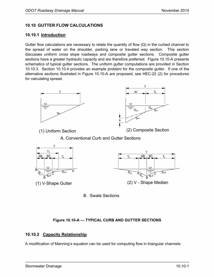
Gutter flow calculations are necessary to relate the quantity of flow (Q) in the curbed channel to the spread of water on the shoulder, parking lane or traveled way section. This section discusses uniform cross slope roadways and composite gutter sections. Composite gutter sections have a greater hydraulic capacity and are therefore preferred. Figure 10.10-A presents schematics of typical gutter sections. The uniform gutter computations are provided in Section 10.10.3. Section 10.10.4 provides an example problem for the composite gutter. If one of the alternative sections illustrated in Figure 10.10-A are proposed, see HEC-22 (2) for procedures for calculating spread.
Figure 10.10-A — TYPICAL CURB AND GUTTER SECTIONS 10.10.2 Capacity Relationship
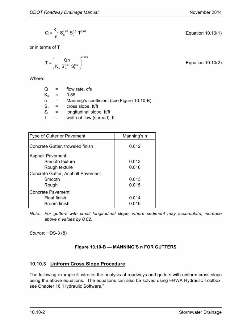
A modification of Manning’s equation can be used for computing flow in triangular channels:
ODOT Roadway Drainage Manual November 2014
10.10-2 Stormwater Drainage
1.67 0.5 2.67ux L
KQ S S T
n= Equation 10.10(1)
or in terms of T
0.375
1.67 0.5u x L
QnT
K S S
=
Equation 10.10(2)
Where:
Q = flow rate, cfs Ku = 0.56 n = Manning’s coefficient (see Figure 10.10-B) Sx = cross slope, ft/ft SL = longitudinal slope, ft/ft T = width of flow (spread), ft
Type of Gutter or Pavement Manning’s n
Concrete Gutter, troweled finish 0.012
Asphalt Pavement: Smooth texture Rough texture
0.013 0.016
Concrete Gutter, Asphalt Pavement Smooth Rough
0.013 0.015
Concrete Pavement Float finish Broom finish
0.014 0.016
Note: For gutters with small longitudinal slope, where sediment may accumulate, increase above n values by 0.02.
Source: HDS-3 (8)
Figure 10.10-B — MANNING’S n FOR GUTTERS 10.10.3 Uniform Cross Slope Procedure
The following example illustrates the analysis of roadways and gutters with uniform cross slope using the above equations. The equations can also be solved using FHWA Hydraulic Toolbox; see Chapter 16 “Hydraulic Software.”
ODOT Roadway Drainage Manual November 2014
Stormwater Drainage 10.10-3
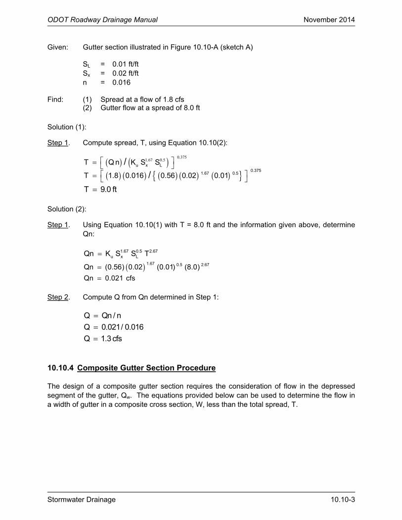
Given: Gutter section illustrated in Figure 10.10-A (sketch A)
SL = 0.01 ft/ft Sx = 0.02 ft/ft n = 0.016
Find: (1) Spread at a flow of 1.8 cfs (2) Gutter flow at a spread of 8.0 ft
Solution (1):
Step 1. Compute spread, T, using Equation 10.10(2):
( ) ( ) 0 3751 67 0 5 .. .
u x LT Q n K S S/ =
( ) ( ) ( ) ( ) ( ){ } 0.3751.67 0.5T 1.8 0.016 0.56 0.02 0.01/ =
T 9.0 ft=
Solution (2):
Step 1. Using Equation 10.10(1) with T = 8.0 ft and the information given above, determine Qn:
1.67 0.5 2.67u x LQn K S S T=
( ) 1.67 0.5 2.67Qn (0.56) 0.02 (0.01) (8.0)=
Qn 0.021 cfs= Step 2. Compute Q from Qn determined in Step 1: Q Qn / n=
Q 0.021/ 0.016=
Q 1.3 cfs= 10.10.4 Composite Gutter Section Procedure
The design of a composite gutter section requires the consideration of flow in the depressed segment of the gutter, Qw. The equations provided below can be used to determine the flow in a width of gutter in a composite cross section, W, less than the total spread, T.

ODOT Roadway Drainage Manual November 2014
10.10-4 Stormwater Drainage
w xo 2.67
w x
S / SE 1/ 1
S / S1 1
T1
W
= + + − −
Equation 10.10(3)
w sQ Q Q= − Equation 10.10(4)
s
o
(1 E )=
− Equation 10.10(5)
Where:
Qw = flow rate in the depressed section of the gutter, cfs Q = gutter flow rate, cfs Qs = flow capacity of the gutter section above the depressed section, cfs Eo = ratio of flow in a chosen width (usually the width of a grate) to total gutter
flow (Qw/Q) Sw = Sx + a/W, ft/ft (see Figure 10.10-A, (sketch A)
The procedure for analyzing composite gutter sections is demonstrated in the following example.
Given: Curb and Gutter section illustrated in Figure 10.10-A (sketch A)
SL = 0.01 ft/ft Sx = 0.02 ft/ft Sw = 0.05 ft/ft W = 2 ft n = 0.016
Find: (1) Gutter flow at a spread (T) = 8.0 ft (2) Spread (T) at a gutter flow (Q) = 2 cfs
Solution (1):
Step 1. Using the cross slope of the depressed gutter (Sw = 0.05), compute “a” and the width of spread from the junction of the gutter and the road to the limit of the spread, Ts:
( )w xS 0.05 a / W S a / 2 0.02 a 0.72 in= = + = + =
sT T – W 8.0 – 2.0= =
s T 6.0 ft=
Step 2. From Equation 10.10(1) (using Ts):

ODOT Roadway Drainage Manual November 2014
Stormwater Drainage 10.10-5
Qsn = Ku Sx1.67 SL
0.5 Ts2.67
Qsn = (0.56) (0.02)1.67 (0.01)0.5 (6.0)2.67 Qsn = 0.0097 cfs Qs = (Qsn)/n = 0.0097/0.016 Qs = 0.61 cfs
Step 3. Determine the gutter flow, Q, using Equation 10.10(3) and 10.10(5):
T/W = 8.0/2 = 4.0 Sw/Sx = 0.05/0.02 = 2.5 Eo = 1 / {1 + [(Sw/Sx)/((1 + (Sw/Sx)/(T/W – 1))2.67 – 1)]} Eo = 1 / {1 + [2.5 / ((1 + (2.5) / (4.0 – 1))2.67 – 1)]} Eo = 0.618 Q = Qs/(1 – Eo) Q = 0.61/(1 – 0.618) Q = 1.6 cfs
Solution (2):
Because the spread cannot be determined by a direct solution, an iterative approach should be used. This approach is provided in HEC-22 (2). If the FHWA Hydraulic Toolbox is used to determine the spread for a given discharge, the results are:
Q = 2.0 cfs T = 8.8 ft Eo = 0.573 Area of flow = 0.834 square ft Depth at curb = 2.83 in with a = 0.72 in
The distribution of the flow is:
Qw = Eo (Q) = 0.573 (2.0) = 1.15 cfs Qs = Q – Qw = 2.0 – 1.15 = 0.85 cfs Ts = T – W = 8.8 – 2 = 6.8 ft

ODOT Roadway Drainage Manual November 2014
10.10-6 Stormwater Drainage
ODOT Roadway Drainage Manual November 2014
Stormwater Drainage 10.11-1
10.11 INLET TYPES
10.11.1 General
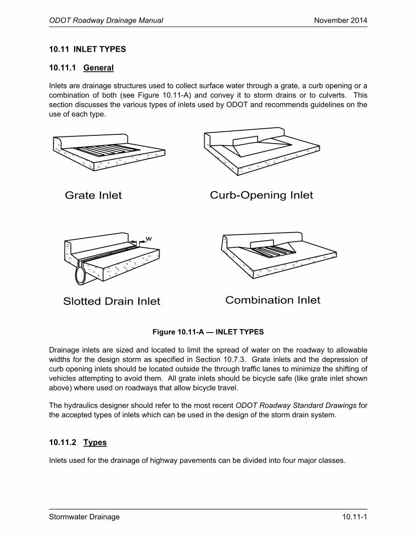
Inlets are drainage structures used to collect surface water through a grate, a curb opening or a combination of both (see Figure 10.11-A) and convey it to storm drains or to culverts. This section discusses the various types of inlets used by ODOT and recommends guidelines on the use of each type.
Figure 10.11-A — INLET TYPES Drainage inlets are sized and located to limit the spread of water on the roadway to allowable widths for the design storm as specified in Section 10.7.3. Grate inlets and the depression of curb opening inlets should be located outside the through traffic lanes to minimize the shifting of vehicles attempting to avoid them. All grate inlets should be bicycle safe (like grate inlet shown above) where used on roadways that allow bicycle travel.
The hydraulics designer should refer to the most recent ODOT Roadway Standard Drawings for the accepted types of inlets which can be used in the design of the storm drain system.
10.11.2 Types
Inlets used for the drainage of highway pavements can be divided into four major classes.
ODOT Roadway Drainage Manual November 2014
10.11-2 Stormwater Drainage
10.11.2.1 Grate Inlets
These inlets consist of an opening in the gutter covered by one or more grates. They are best suited for use on continuous grades. Because they are susceptible to clogging with debris, the use of standard grate inlets at sag points should be limited to minor sag point locations without debris potential. Special-design (oversize) grate inlets can be used at major sag points if sufficient capacity is provided for clogging. Otherwise, flanking inlets are needed.
10.11.2.2 Curb-Opening Inlets
These inlets provide openings in the curb covered by a top slab. Curb-opening inlets are preferred at sag points because they can convey large quantities of water and debris. They may also be a viable alternative to grates in many locations where grates may be hazardous for pedestrians or bicyclists. They are generally not the first choice for use on continuous grades because of their poor hydraulic capacity.
10.11.2.3 Combination Inlets
Various types of combination inlets are in use. Curb-opening and grate combinations are common, some with the curb opening upstream of the grate and some with the curb opening adjacent to the grate. The gutter grade, cross slope and proximity of the inlets to each other are significant factors when selecting this type of inlet. Combination inlets may be desirable in sags because they can provide additional capacity in the event of plugging.
10.11.2.4 Slotted Drain Inlets
These inlets consist of a slotted opening with bars perpendicular to the opening. Slotted inlets function as weirs because the flow usually enters perpendicular to the slot. They can be used to intercept sheet flow, collect gutter flow with or without curbs, modify existing systems to accommodate roadway widening or increased runoff and reduce ponding depth and spread at grate inlets.
Slotted corrugated metal pipes may be used in median crossovers and, at times, in curb and gutter sections where large volumes of water need to be picked up. Slotted reinforced concrete pipe may be used as a median drain. HEC-22 (2) contains design guidance.
10.11.3 Drop Inlets
A drop inlet provides a base for the drainage grate. Basically, the drop inlet represents the below-pavement structure (or basin) to collect the storm drainage from the inlets and to convey the drainage to the underground piping system.
ODOT Roadway Drainage Manual November 2014
Stormwater Drainage 10.12-1
10.12 INLET LOCATION, SPACING AND CAPACITY
10.12.1 Location
There are a number of locations where inlets may be necessary without regard to contributing drainage area. These locations should be marked on the plans prior to any hydraulic computations regarding discharge, water spread, inlet capacity or bypass. Examples of such locations are:
• Inlets on grade should be spaced at a maximum shown in Table 10.4-A.
• Inlets should be placed on the upstream side of bridge approaches.
• Inlets should be placed at all low points in the gutter grade.
• Inlets should be placed upstream of intersecting streets.
• Inlets should be placed on the upstream side of a driveway entrance, curb-cut ramp or pedestrian crosswalk even if the hydraulic analysis places the inlet further down grade or within the feature.
• Inlets should be placed upstream of median breaks.
• Inlets should be placed to capture flow from intersecting streets before it reaches the major highway.
• Flanking inlets in sag vertical curves are standard practice. See Section 10.12.9.
• Inlets should be placed to prevent water from sheeting across the highway (i.e., place the inlet before the superelevation transition begins).
• Inlets should not be located in the path where pedestrians walk.
10.12.2 Spacing Process
Locate inlets from the crest and work downgrade to the sag points. The location of the first inlet from the crest can be found by determining the length of pavement and the area in back of the curb sloping toward the roadway that will generate the design runoff. The design runoff can be computed as the maximum allowable flow in the curbed channel that will meet the design frequency and allowable water spread. Where the contributing drainage area consists of a strip of land parallel to and including a portion of the highway, the location of the first inlet can be calculated as follows:
t43,560 QL
CiW= Equation 10.12(1)
ODOT Roadway Drainage Manual November 2014
10.12-2 Stormwater Drainage
Where:
L = distance from the crest, ft Qt = maximum allowable flow, cfs C = composite runoff coefficient for contributing drainage area W = width of contributing drainage area, ft i = rainfall intensity for design frequency, in/h
Equation 10.12(1) is an alternate form of the Rational Equation. If the drainage area contributing to the first inlet from the crest is irregular in shape, trial and error may be necessary to match a design flow with the maximum allowable flow.
To space successive downgrade inlets, it is necessary to compute the amount of flow that will be intercepted by the inlet (Qi) and subtract it from the total gutter flow to compute the bypass. The bypass from the first inlet is added to the computed flow to the second inlet, the total of which must be less than the maximum allowable flow dictated by the allowable water spread. Figure 10.14-A (see Section 10.14) is an inlet spacing computation sheet that can be used to record the spacing calculations. However, inlet calculations are usually accomplished with software.
FHWA has investigated the inlet interception capacity of all types of grate inlets, slotted drain inlets, curb-opening inlets and combination inlets. HEC-22 (2) or the FHWA Hydraulic Toolbox (see Chapter 16 “Hydraulic Software”) may be used to analyze the flow in gutters and the interception capacity of all types of inlets on continuous grades and sags. Both uniform and composite cross slopes can be analyzed.
10.12.3 Grate Inlets on Grade
The capacity of a grate inlet depends upon its geometry, cross slope, longitudinal slope, total gutter flow, depth of flow and pavement roughness. The depth of water next to the curb is the major factor in the interception capacity of both gutter inlets and curb-opening inlets. At low velocities, all of the water flowing in the section of gutter occupied by the grate (frontal flow), is intercepted by grate inlets and a small portion of the flow along the length of the grate (side flow) is intercepted. On steep longitudinal slopes, a portion of the frontal flow may tend to splash over the end of the grate for some grates.
The ratio of frontal flow to total gutter flow, Eo, for a straight cross slope is given by the following equation:
( )2.67
o wE Q / Q 1 1 W / T= = − − Equation 10.12(2)
Where:
Q = total gutter flow, cfs Qw = flow in width W, cfs W = width of depressed gutter or grate, ft T = total spread of water in the gutter, ft
ODOT Roadway Drainage Manual November 2014
Stormwater Drainage 10.12-3
The ratio of side flow, Qs, to total gutter flow is:
s w oQ / Q 1 Q / Q 1 E= − = − Equation 10.12(3)
The ratio of frontal flow intercepted to total frontal flow, Rf, is expressed by the following equation:
f oR 1 0.09 (V V )= − − Equation 10.12(4)
Where:
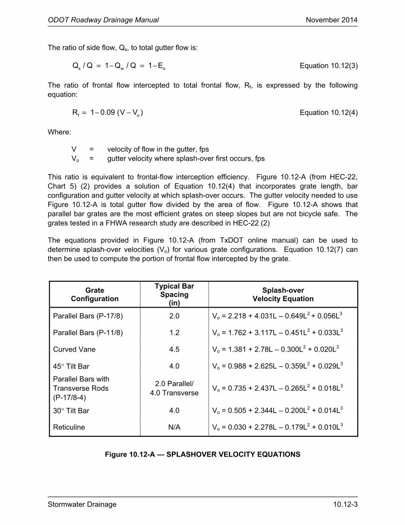
V = velocity of flow in the gutter, fps Vo = gutter velocity where splash-over first occurs, fps This ratio is equivalent to frontal-flow interception efficiency. Figure 10.12-A (from HEC-22, Chart 5) (2) provides a solution of Equation 10.12(4) that incorporates grate length, bar configuration and gutter velocity at which splash-over occurs. The gutter velocity needed to use Figure 10.12-A is total gutter flow divided by the area of flow. Figure 10.12-A shows that parallel bar grates are the most efficient grates on steep slopes but are not bicycle safe. The grates tested in a FHWA research study are described in HEC-22 (2)
The equations provided in Figure 10.12-A (from TxDOT online manual) can be used to determine splash-over velocities (Vo) for various grate configurations. Equation 10.12(7) can then be used to compute the portion of frontal flow intercepted by the grate.
Grate Configuration
Typical Bar Spacing
(in)
Splash-over Velocity Equation
Parallel Bars (P-17/8) 2.0 Vo = 2.218 + 4.031L – 0.649L2 + 0.056L3
Parallel Bars (P-11/8) 1.2 Vo = 1.762 + 3.117L – 0.451L2 + 0.033L3
Curved Vane 4.5 Vo = 1.381 + 2.78L – 0.300L2 + 0.020L3
45° Tilt Bar 4.0 Vo = 0.988 + 2.625L – 0.359L2 + 0.029L3
Parallel Bars with Transverse Rods (P-17/8-4)
2.0 Parallel/ 4.0 Transverse
Vo = 0.735 + 2.437L – 0.265L2 + 0.018L3
30° Tilt Bar 4.0 Vo = 0.505 + 2.344L – 0.200L2 + 0.014L3
Reticuline N/A Vo = 0.030 + 2.278L – 0.179L2 + 0.010L3
Figure 10.12-A — SPLASHOVER VELOCITY EQUATIONS
ODOT Roadway Drainage Manual November 2014
10.12-4 Stormwater Drainage
The ratio of side flow intercepted to total side flow, Rs, or side-flow interception efficiency, is expressed by:
( )1.8 2.3s xR 1 / 1 0.15V / S L = + Equation 10.12(5)
Where:
V = velocity of flow in gutter, fps L = length of the grate, ft Sx = cross slope, ft/ft
The efficiency, E, of a grate is expressed as:
f o s oE R E R (1 E )= + − Equation 10.12(6)
The interception capacity of a grate inlet on grade is equal to the efficiency of the grate multiplied by the total gutter flow:
i f o s oQ EQ Q[R E R (1 E )]= = + − Equation 10.12(7)
Composite Gutter and Grate Example
Given: Given the gutter section from Section 10.10.4:
T = 8.0 ft SL = 0.01 ft/ft W = 2.0 ft Sx = 0.02 ft/ft n = 0.016 Sw = 0.05 ft/ft (continuous gutter depression, a = 0.72 in)
Find: The interception capacity of a grate that has outside dimensions of 1.5 ft by 3 ft and has 11 vanes. The vanes are 2-in high and at a 45-degree angle to vertical. (Note: Although this is a combination inlet, the grate provides all of the capacity and the curb opening provides for debris).
Solution: From Section 10.10.4
Eo = 0.618 Q = 1.6 cfs
Step 1. Compute the average gutter velocity:
V = Q/A = 1.6/A A = 0.5T2Sx + 0.5aW A = 0.5(8.0)2 (0.02) + 0.5(0.06)(2.0) = 0.64 + 0.06 A = 0.70 square ft V = 1.6/0.70 = 2.29 fps
Step 2. Determine the frontal flow efficiency using Figure 10.12-B:
Rf = 1.0
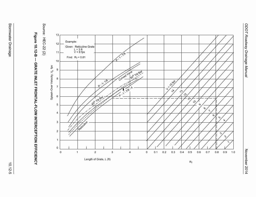
OD
OT
Road
way D
rainage Manual
N
ovem
ber 2014
Storm
water D
rainage 10.12-5
Source: H
EC
-22 (2)
Fig
ure 10.12-B
— G
RA
TE
INL
ET
FR
ON
TA
L-F
LO
W IN
TE
RC
EP
TIO
N E
FF
ICIE
NC
Y

ODOT Roadway Drainage Manual November 2014
10.12-6 Stormwater Drainage
Step 3. Determine the side flow efficiency using Equation 10.12(5):
Rs = 1/[1+ (0.15 V1.8) / (Sx L2.3)]
Rs = 1/[1+ (0.15) (2.29)1.8 / [(0.02) (3.0)2.3] Rs = 0.27
Step 4. Compute the interception capacity using Equation 10.12(7). (Because the grate is only 1.50 ft (18-in) wide, replace Eo with Eo = Eo (A′w/Aw) where Aw is the area of flow over the 2-ft gutter and A′w is the area of flow over the grate):
oE′ = Eo (A′w/Aw) = 0.618(0.27/0.34) = 0.491 Qi = Q[Rf Eo + Rs (1 – Eo)] = (1.6)[(1.0)(0.491) + (0.27)(1 – 0.491)] = 1.6 (0.491 + 0.137) = 1.6(0.628) = 1.00 cfs E = Qi/Q = 1.00/1.6 = 0.625 or 63%
The calculations show that the inlet is 63% efficient and captures 1.0 cfs while 0.60 cfs is bypassed. The FHWA Hydraulic Toolbox gives similar results.
10.12.4 Grate Inlets in Sag
Although curb-opening inlets are generally preferred to grate inlets at a sag, grate inlets can be used successfully. For minor sag points where debris potential is limited, grate inlets without a curb-opening inlet can be utilized. An example of a minor sag point might be on a ramp as it joins a mainline. Curb-opening inlets in addition to a grate are preferred at sag points where debris is likely, such as on a city street (see Section 10.12.6). For major sag points, such as on divided high-speed highways, a curb-opening inlet is preferable to a grate inlet because of its hydraulic capacity and debris-handling capabilities. When grates are used, it is good practice to assume that half the grate is clogged with debris.
Where significant ponding can occur, in locations such as underpasses and in sag vertical curves in depressed sections, it is good engineering practice to place a minimum of one flanking inlet on each side of the sag point inlet. The flanking inlets should be placed so that they will limit spread on low-gradient approaches to the low point and act in relief of the inlet at the low point if it should become clogged or if the allowable spread is exceeded. Section 10.12.10 presents a further discussion and methodology.
A grate inlet in a sag operates as a weir up to depths dependent on the size of the grate and as an orifice at greater depths. Grates of larger dimension will operate as weirs to greater depths than smaller grates.
The capacity of a grate inlet operating as a weir is:
1.5i wQ C Pd= Equation 10.12(8)
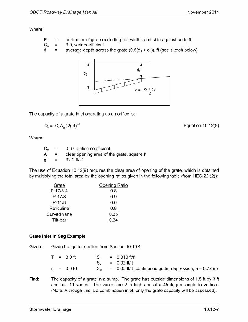
ODOT Roadway Drainage Manual November 2014
Stormwater Drainage 10.12-7
Where:
P = perimeter of grate excluding bar widths and side against curb, ft Cw = 3.0, weir coefficient d = average depth across the grate (0.5(d1 + d2)), ft (see sketch below)
The capacity of a grate inlet operating as an orifice is:
( )0.5
i o gQ C A 2gd= Equation 10.12(9)
Where:
Co = 0.67, orifice coefficient Ag = clear opening area of the grate, square ft g = 32.2 ft/s2
The use of Equation 10.12(9) requires the clear area of opening of the grate, which is obtained by multiplying the total area by the opening ratios given in the following table (from HEC-22 (2)):
Grate Opening Ratio P-17/8-4 0.8 P-17/8 0.9 P-11/8 0.6
Reticuline 0.8 Curved vane 0.35
Tilt-bar 0.34
Grate Inlet in Sag Example
Given: Given the gutter section from Section 10.10.4:
T = 8.0 ft SL = 0.010 ft/ft Sx = 0.02 ft/ft n = 0.016 Sw = 0.05 ft/ft (continuous gutter depression, a = 0.72 in)
Find: The capacity of a grate in a sump. The grate has outside dimensions of 1.5 ft by 3 ft and has 11 vanes. The vanes are 2-in high and at a 45-degree angle to vertical. (Note: Although this is a combination inlet, only the grate capacity will be assessed).
ODOT Roadway Drainage Manual November 2014
10.12-8 Stormwater Drainage
Solution: From Section 10.10.4:
Eo = 0.618 Q = 1.6 cfs
Solution:
Step 1. Determine the required grate perimeter.
Depth at curb, d2:
d2 = TSx + a = (8) (0.02) + 0.72/12 = 0.16 + 0.06 d2 = 0.22 ft
Average depth over grate:
d = d2 – ((grate width)/2)Sw d = 0.22 – (1.5/2)(0.05) d = 0.18 ft with no clogging d = 0.20 ft with 50% clogging (assume that the upper half is clogged so that only
25% of the 1.5-ft width is subtracted to determine average depth)
From Equation 10.12(8):
P = Qi / [Cw d1.5] P = (1.6)/[(3.0)(0.20)1.5] P = 5.96 ft (use 6 ft)
Assuming 50% clogging along the grate length (i.e., width is reduced by 50%):
Peffective = 6.0 = (0.5)(2)W + L if W = 1.5 ft, then L = 4.5 ft
The grate is a 1.5 ft by 3 ft grate:
Peffective = (0.5)(1.5)(2.0) + (3) Peffective = 4.5 ft (one grate) Peffective = 7.5 ft (2 grates) > 6 ft needed, OK
Step 2. Check depth of flow at curb using Equation 10.12(8) using two grates.
d = [Q/(Cw P)]0.67 d = [1.6/(3.0) (7.5)]0.67 d = 0.17 ft or 2 in
Therefore, OK Step 3. Check depth of flow assuming orifice flow, Equation 10.12(9).
Ag = 0.75(3)(0.34) = 0.765 square ft (clogged area is further reduced by opening ratio)
ODOT Roadway Drainage Manual November 2014
Stormwater Drainage 10.12-9
Qi = Co Ag (2gd)0.5 = 0.67(0.765)(64.4d)0.5 = 1.6 cfs d = 0.15 ft (1 grate) d = 0.04 ft (2 grates) Because these depths are lower than those in Step 2, orifice flow does not occur.
10.12.5 Curb Opening Inlets on Grade
Curb-opening inlets are effective in the drainage of highway pavements where flow depth at the curb is sufficient for the inlet to perform efficiently. Curb openings are relatively free of clogging tendencies and offer little interference to traffic operation. They are a viable alternative to grates in many locations where grates would be in traffic lanes or would be hazardous for pedestrians or bicyclists.
The length of a curb-opening inlet required for total interception of gutter flow on a pavement section with a straight cross slope is expressed by:
( )0.30.42 0.6T L xL KQ S (1/ (nS ))= Equation 10.12(10)
Where:
K = 0.6 LT = curb-opening length required to intercept 100% of the gutter flow, ft
The efficiency of curb-opening inlets shorter than the length required for total interception is expressed by:
1.8TE 1 (1 L / L )= − − Equation 10.12(11)
Where:
L = curb-opening length, ft
The length of inlet required for total interception by depressed curb-opening inlets or curb openings in depressed gutter sections or for a continuously depressed gutter (composite gutter) can be found by the use of an equivalent cross slope, Se, in Equation 10.12(12):
e x w oS S S E′= + Equation 10.12(12)
Where:
wS′ = (a/12W) = Sw – Sx = cross slope of the gutter measured from the cross slope
of the pavement, ft/ft
a = gutter depression, in
Eo = ratio of flow in the depressed section to total gutter flow. It is determined by the gutter configuration upstream of the inlet (see Section 10.10.4).
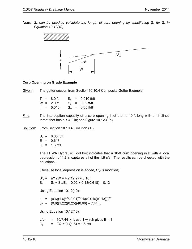
ODOT Roadway Drainage Manual November 2014
10.12-10 Stormwater Drainage
Note: Se can be used to calculate the length of curb opening by substituting Se for Sx in Equation 10.12(10).
Curb Opening on Grade Example
Given: The gutter section from Section 10.10.4 Composite Gutter Example:
T = 8.0 ft SL = 0.010 ft/ft W = 2.0 ft Sx = 0.02 ft/ft n = 0.016 Sw = 0.05 ft/ft
Find: The interception capacity of a curb opening inlet that is 10-ft long with an inclined throat that has a = 4.2 in; see Figure 10.12-C(b).
Solution: From Section 10.10.4 (Solution (1)):
Sw = 0.05 ft/ft Eo = 0.618 Q = 1.6 cfs
The FHWA Hydraulic Tool box indicates that a 10-ft curb opening inlet with a local depression of 4.2 in captures all of the 1.6 cfs. The results can be checked with the equations:
(Because local depression is added, S′w is modified)
S′w = a/12W = 4.2/12(2) = 0.18 Se = Sx + S′w Eo = 0.02 + 0.18(0.618) = 0.13
Using Equation 10.12(10):
LT = (0.6)(1.6)0.42(0.01)0.3(1/((0.016)(0.13)))0.6 LT = (0.6)(1.22)(0.25)(40.66) = 7.44 ft
Using Equation 10.12(13):
L/LT = 10/7.44 > 1, use 1 which gives E = 1 Qi = EQ = (1)(1.6) = 1.6 cfs
ODOT Roadway Drainage Manual November 2014
Stormwater Drainage 10.12-11
10.12.6 Curb-Opening Inlets in Sag
The capacity of a curb-opening inlet in a sag depends on the water depth at the curb, the curb-opening length and the height of the curb opening. The inlet operates as a weir to depths equal to the curb-opening height and as an orifice at depths greater than 1.4 times the opening height. At depths between 1.0 and 1.4 times the opening height, flow is in a transition stage. See Figure 10.12-C for a definition sketch.
The equation for the interception capacity of a depressed curb-opening inlet operating as a weir is:
( ) 1.5i WQ C L 1.8W d= + Equation 10.12(13)
Where:
CW = 2.3 (with depression)
L = length of curb opening, ft
W = width of depression, ft
d = depth of water at curb measured from the normal cross slope, ft (i.e., d = TSx
for a uniform gutter and d = a + TSx for a composite section
The weir equation is applicable to depths at the curb less than or equal to the height of the opening plus the depth of the depression (D ≤ h + a).
The weir equation for curb-opening inlets without a depression becomes:
1.5i WQ C Ld= Equation 10.12(14)
CW = 3.0 (without depression)
The depth limitation for operation as a weir becomes d ≤ h.
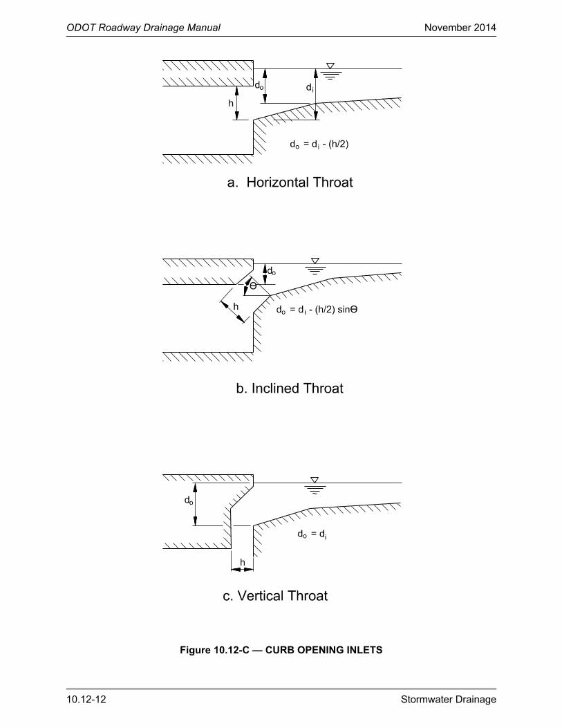
ODOT Roadway Drainage Manual November 2014
10.12-12 Stormwater Drainage
Figure 10.12-C — CURB OPENING INLETS
ODOT Roadway Drainage Manual November 2014
Stormwater Drainage 10.12-13
Curb-opening inlets operate as orifices at depths greater than approximately 1.4 times the height of curb opening (1.4h). The interception capacity can be computed by Equation 10.12(15). The depth at the inlet includes any gutter depression:
( ) 0.5
i o oQ C hL 2g d = Equation 10.12(15)
Where:
Co = orifice coefficient (0.67) do = effective head on the center of the orifice throat, ft (see Figure 10.12-C) h = height of curb-opening orifice, ft L = length of orifice opening, ft di = depth at lip of curb opening, ft = d + a/12 = TSx + a/12 (a = local depression)
The following applies to the local depression:
1. Weir Flow. a = local gutter depression, in. This depression is used to determine if the inlet is in weir flow only. Local depression is only used to check if the orifice is submerged.
2. Orifice Flow. a = local depression at curb opening, in. This depression is used in orifice flow inlet capacity computations.
Curb-Opening in Sag Example
Given: The curb opening inlet with an inclined throat in a sump location with a curb and gutter for approach. Use Composite gutter (Section 10.8.4) Example gutter flow (Q = 1.6 cfs) for T = 8.0 ft and a = 0.72 in (local gutter depression), and:
L = 10 ft h = 0.48 ft a = 4.2 in (local depression at curb opening) W = 2 ft
Find: Qi
Solution:
Step 1. Determine depth in gutter at curb, d.
d = d + a (Use “a” for gutter depression) d = TSx + a d = (0.02)(8.0) + 0.72/12 d = 0.22 ft d < (h + a) = 0.48 + 0.06 = 0.54 ft; therefore, weir flow controls
Step 2. Use Equation 10.12(15) to find Qi.
P = L + 1.8 W
ODOT Roadway Drainage Manual November 2014
10.12-14 Stormwater Drainage
P = 10 + (1.8)(2) P = 13.6 ft Qi = Cw (L + 1.8 W) d1.5
Qi = (2.3) (13.6) (0.22)1.5 Qi = 3.2 cfs
The FHWA Hydraulic Toolbox also indicates that the inlet is in weir flow and will accept all the flow. By trial and error, the flow must be 51.4 cfs for this inlet to operate in orifice flow. At this flow, the depth at the curb is 8.3 in.
10.12.7 Combination Inlet on Grade
The interception capacity of a combination inlet consisting of a curb opening and grate placed side-by-side is no greater than that of the grate alone. Capacity is computed by neglecting the curb opening. A combination inlet is sometimes used with a part of the curb opening placed upstream of the grate. The curb opening in such an installation intercepts debris which might otherwise clog the grate and is called a “sweeper” inlet. A sweeper combination inlet has an interception capacity equal to the sum of the curb opening upstream of the grate plus the grate capacity, except that the frontal flow and thus the interception capacity of the grate is reduced by interception by the curb opening.
10.12.8 Combination Inlet in Sag
Combination inlets consisting of a grate and a curb opening are considered advisable for use in sags where hazardous ponding can occur. Equal length inlets refer to a grate inlet placed alongside a curb opening inlet, both of which have the same length. The interception capacity of the equal length combination inlet is essentially equal to that of a grate alone in weir flow. In orifice flow, the capacity of the equal length combination inlet is equal to the capacity of the grate plus the capacity of the curb opening. If two grates are added to the 10-ft curb opening in Section 10.12.6 and the inlet is treated as a sweeper inlet, the FHWA Hydraulic Toolbox shows that the combination will accommodate 44 cfs before going into orifice flow. This example is provided only to demonstrate the potential additional capacity that can be gained using inlets in combination. The tilt-bar grate used in the examples should not be used in a sump condition, because it is designed to be used on a grade. A better use of the two tilt-bar grates is to use them upstream of the sump as flanking inlets (see Section 10.12.9).
10.12.9 Flanking Inlets
At major sag points where significant ponding may occur, such as underpasses or sag vertical curves in depressed sections, it is recommended practice to place a minimum of one flanking inlet on each side of the inlet at the sag point. The flanking inlets can be located so that they will function before the water spread exceeds the allowable spread at the sump location. The flanking inlets should be located so that they will receive all of the flow when the primary inlet at the bottom of the sag is clogged. They should do this without exceeding the allowable spread at the bottom of the sag.
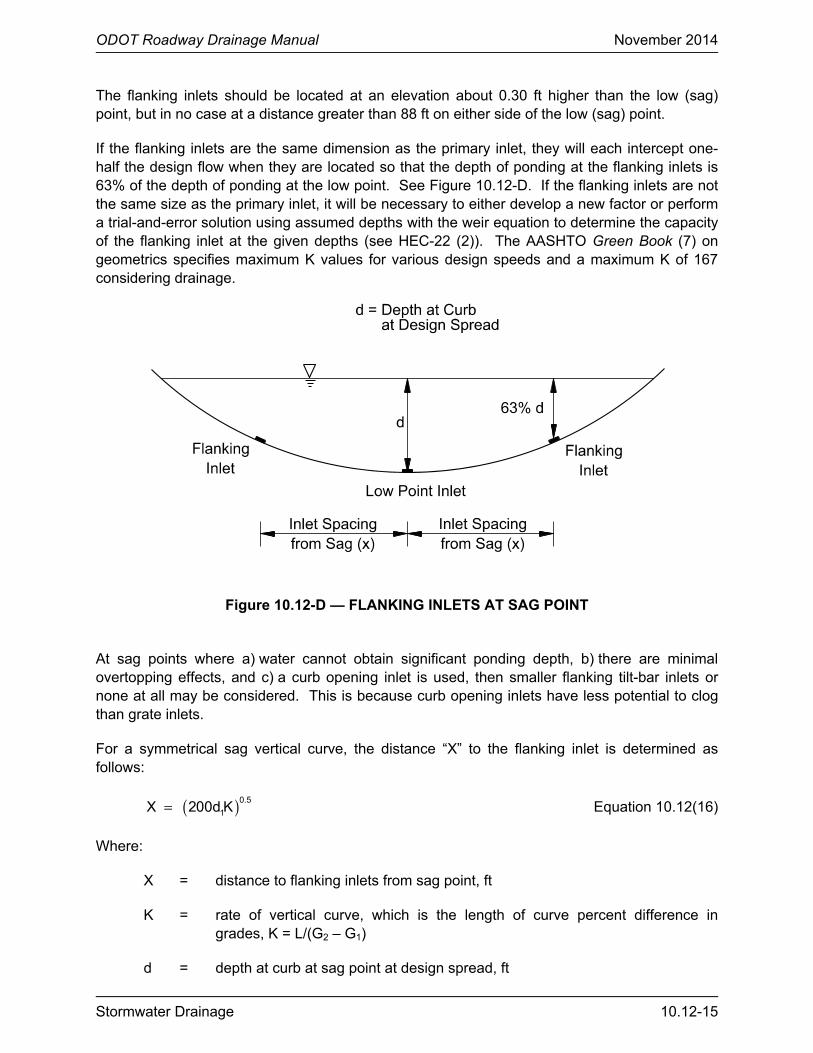
ODOT Roadway Drainage Manual November 2014
Stormwater Drainage 10.12-15
The flanking inlets should be located at an elevation about 0.30 ft higher than the low (sag) point, but in no case at a distance greater than 88 ft on either side of the low (sag) point.
If the flanking inlets are the same dimension as the primary inlet, they will each intercept one-half the design flow when they are located so that the depth of ponding at the flanking inlets is 63% of the depth of ponding at the low point. See Figure 10.12-D. If the flanking inlets are not the same size as the primary inlet, it will be necessary to either develop a new factor or perform a trial-and-error solution using assumed depths with the weir equation to determine the capacity of the flanking inlet at the given depths (see HEC-22 (2)). The AASHTO Green Book (7) on geometrics specifies maximum K values for various design speeds and a maximum K of 167 considering drainage.
Figure 10.12-D — FLANKING INLETS AT SAG POINT At sag points where a) water cannot obtain significant ponding depth, b) there are minimal overtopping effects, and c) a curb opening inlet is used, then smaller flanking tilt-bar inlets or none at all may be considered. This is because curb opening inlets have less potential to clog than grate inlets.
For a symmetrical sag vertical curve, the distance “X” to the flanking inlet is determined as follows:
( )0.5
1X 200d K= Equation 10.12(16)
Where:
X = distance to flanking inlets from sag point, ft
K = rate of vertical curve, which is the length of curve percent difference in grades, K = L/(G2 – G1)
d = depth at curb at sag point at design spread, ft
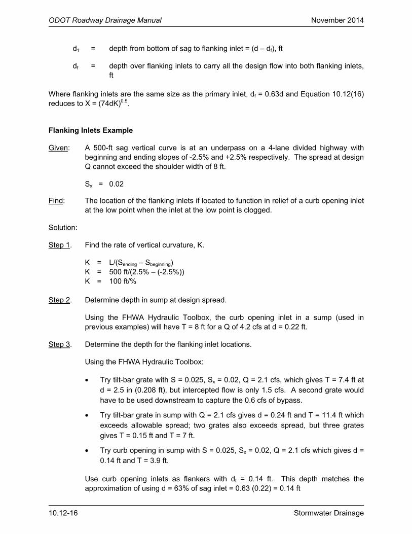
ODOT Roadway Drainage Manual November 2014
10.12-16 Stormwater Drainage
d1 = depth from bottom of sag to flanking inlet = (d – df), ft
df = depth over flanking inlets to carry all the design flow into both flanking inlets, ft
Where flanking inlets are the same size as the primary inlet, df = 0.63d and Equation 10.12(16) reduces to X = (74dK)0.5.
Flanking Inlets Example
Given: A 500-ft sag vertical curve is at an underpass on a 4-lane divided highway with beginning and ending slopes of -2.5% and +2.5% respectively. The spread at design Q cannot exceed the shoulder width of 8 ft.
Sx = 0.02
Find: The location of the flanking inlets if located to function in relief of a curb opening inlet at the low point when the inlet at the low point is clogged.
Solution:
Step 1. Find the rate of vertical curvature, K.
K = L/(Sending – Sbeginning) K = 500 ft/(2.5% – (-2.5%)) K = 100 ft/%
Step 2. Determine depth in sump at design spread.
Using the FHWA Hydraulic Toolbox, the curb opening inlet in a sump (used in previous examples) will have T = 8 ft for a Q of 4.2 cfs at d = 0.22 ft.
Step 3. Determine the depth for the flanking inlet locations.
Using the FHWA Hydraulic Toolbox:
• Try tilt-bar grate with S = 0.025, Sx = 0.02, Q = 2.1 cfs, which gives T = 7.4 ft at d = 2.5 in (0.208 ft), but intercepted flow is only 1.5 cfs. A second grate would have to be used downstream to capture the 0.6 cfs of bypass.
• Try tilt-bar grate in sump with Q = 2.1 cfs gives d = 0.24 ft and T = 11.4 ft which exceeds allowable spread; two grates also exceeds spread, but three grates gives T = 0.15 ft and T = 7 ft.
• Try curb opening in sump with S = 0.025, Sx = 0.02, Q = 2.1 cfs which gives d = 0.14 ft and T = 3.9 ft.
Use curb opening inlets as flankers with df = 0.14 ft. This depth matches the approximation of using d = 63% of sag inlet = 0.63 (0.22) = 0.14 ft

ODOT Roadway Drainage Manual November 2014
Stormwater Drainage 10.12-17
Step 4. Determine distance to flanking inlets.
d1 = 0.22 – 0.14 = 0.08 ft X = (200d1K)0.5 = {(200)(0.08)(100)}0.5 = 40.0 ft or X = (74dK)0.5 = {(74)(0.22)(100)}0.5 = 40.3 ft Therefore, flanking inlet spacing = 40 ft from the low point in the sag.
10.12.10 Inlet Spacing Computations
To design the location of the inlets for a given project, information such as a layout or plan sheet suitable for outlining drainage areas, road profiles, typical cross sections, grading cross sections, superelevation diagrams and contour maps are necessary. The inlet computation sheet, Figure 10.12-E, should be used to document the computations. A step-by-step procedure is as follows:
Step 1. Complete the blanks on top of the sheet to identify the job by project number, route, date and your initials.
Step 2. Mark on the plan the location of inlets that are necessary without consideration of any specific drainage area (see Section 10.12.1).
Step 3. Start at a high point, at one end of the project if possible and work towards the low point. Then, begin at the next high point and work backwards toward the same low point.
Step 4. To begin the process, select a trial drainage area that is approximately 300 ft to 500 ft below the high point and outline the area on the plan. Include any area that may drain over the curb and onto the roadway. Use drainage area maps. Where practical, drainage from large areas behind the curb should be intercepted before it reaches the roadway or gutter.
Step 5.
Col. 1 Col. 2 Col. 19
Describe the location of the proposed inlet by number and station in Columns 1 and 2. Identify the curb and gutter type in the Remarks, Column 19. A sketch of the cross section should be provided in the open area of the computation sheet.
Step 6.
Col. 3 Compute the drainage area in acres outlined in Step 4 and record in Column 3.
Step 7. Col. 4 Determine the runoff coefficient C for the drainage area. Select a C value or compute a weighted C value based on area and cover type and record the value in Column 4.
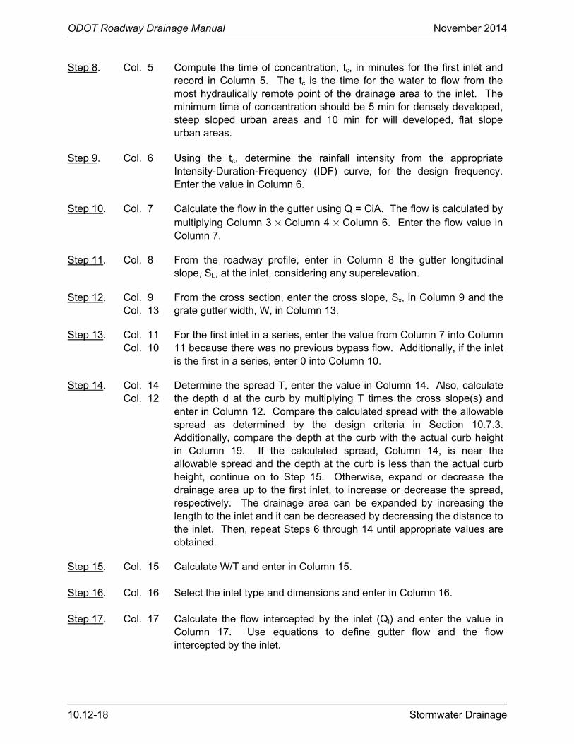
ODOT Roadway Drainage Manual November 2014
10.12-18 Stormwater Drainage
Step 8.
Col. 5 Compute the time of concentration, tc, in minutes for the first inlet and record in Column 5. The tc is the time for the water to flow from the most hydraulically remote point of the drainage area to the inlet. The minimum time of concentration should be 5 min for densely developed, steep sloped urban areas and 10 min for will developed, flat slope urban areas.
Step 9.
Col. 6 Using the tc, determine the rainfall intensity from the appropriate Intensity-Duration-Frequency (IDF) curve, for the design frequency. Enter the value in Column 6.
Step 10.
Col. 7 Calculate the flow in the gutter using Q = CiA. The flow is calculated by multiplying Column 3 × Column 4 × Column 6. Enter the flow value in Column 7.
Step 11.
Col. 8 From the roadway profile, enter in Column 8 the gutter longitudinal slope, SL, at the inlet, considering any superelevation.
Step 12.
Col. 9 Col. 13
From the cross section, enter the cross slope, Sx, in Column 9 and the grate gutter width, W, in Column 13.
Step 13.
Col. 11 Col. 10
For the first inlet in a series, enter the value from Column 7 into Column 11 because there was no previous bypass flow. Additionally, if the inlet is the first in a series, enter 0 into Column 10.
Step 14.
Col. 14 Col. 12
Determine the spread T, enter the value in Column 14. Also, calculate the depth d at the curb by multiplying T times the cross slope(s) and enter in Column 12. Compare the calculated spread with the allowable spread as determined by the design criteria in Section 10.7.3. Additionally, compare the depth at the curb with the actual curb height in Column 19. If the calculated spread, Column 14, is near the allowable spread and the depth at the curb is less than the actual curb height, continue on to Step 15. Otherwise, expand or decrease the drainage area up to the first inlet, to increase or decrease the spread, respectively. The drainage area can be expanded by increasing the length to the inlet and it can be decreased by decreasing the distance to the inlet. Then, repeat Steps 6 through 14 until appropriate values are obtained.
Step 15.
Col. 15
Calculate W/T and enter in Column 15.
Step 16.
Col. 16
Select the inlet type and dimensions and enter in Column 16.
Step 17.
Col. 17
Calculate the flow intercepted by the inlet (Qi) and enter the value in Column 17. Use equations to define gutter flow and the flow intercepted by the inlet.
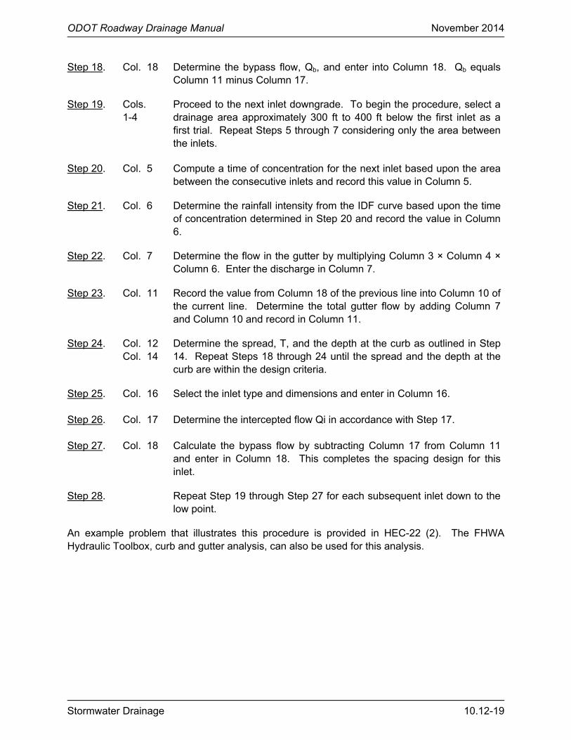
ODOT Roadway Drainage Manual November 2014
Stormwater Drainage 10.12-19
Step 18.
Col. 18 Determine the bypass flow, Qb, and enter into Column 18. Qb equals Column 11 minus Column 17.
Step 19. Cols. 1-4
Proceed to the next inlet downgrade. To begin the procedure, select a drainage area approximately 300 ft to 400 ft below the first inlet as a first trial. Repeat Steps 5 through 7 considering only the area between the inlets.
Step 20.
Col. 5 Compute a time of concentration for the next inlet based upon the area between the consecutive inlets and record this value in Column 5.
Step 21.
Col. 6
Determine the rainfall intensity from the IDF curve based upon the time of concentration determined in Step 20 and record the value in Column 6.
Step 22. Col. 7 Determine the flow in the gutter by multiplying Column 3 × Column 4 × Column 6. Enter the discharge in Column 7.
Step 23. Col. 11 Record the value from Column 18 of the previous line into Column 10 of the current line. Determine the total gutter flow by adding Column 7 and Column 10 and record in Column 11.
Step 24.
Col. 12 Col. 14
Determine the spread, T, and the depth at the curb as outlined in Step 14. Repeat Steps 18 through 24 until the spread and the depth at the curb are within the design criteria.
Step 25.
Col. 16 Select the inlet type and dimensions and enter in Column 16.
Step 26.
Col. 17 Determine the intercepted flow Qi in accordance with Step 17.
Step 27.
Col. 18 Calculate the bypass flow by subtracting Column 17 from Column 11 and enter in Column 18. This completes the spacing design for this inlet.
Step 28. Repeat Step 19 through Step 27 for each subsequent inlet down to the low point.
An example problem that illustrates this procedure is provided in HEC-22 (2). The FHWA Hydraulic Toolbox, curb and gutter analysis, can also be used for this analysis.
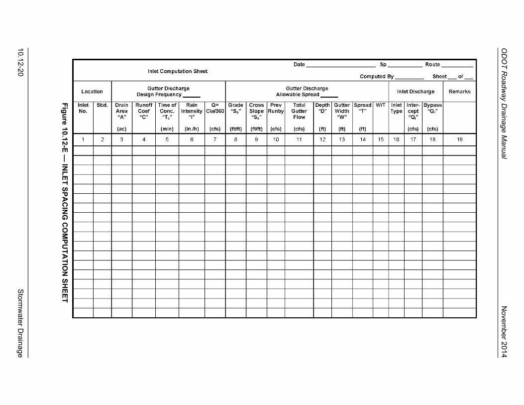
OD
OT
Road
way D
rainage Manual
N
ovem
ber 2014
10.12-20 S
tormw
ater Drainage
Fig
ure 10.12-E
— IN
LE
T S
PA
CIN
G C
OM
PU
TA
TIO
N S
HE
ET
ODOT Roadway Drainage Manual November 2014
Stormwater Drainage 10.13-1
10.13 ODOT STORM DRAIN PRACTICE
10.13.1 Pipe Material
The following documents state practices (not related to the hydraulic analysis) for the underground portion of a storm drainage system.
10.13.1.1 Minimum Pipe Size
The typical minimum round pipe size is 18 in. In special cases, a 12-in pipe may be used where it is not possible/practical to provide an 18-in pipe. Justification for a 12-in pipe should be documented. Pipe sizes typically increase in 3-in increments, but all sizes may not have a commensurate ODOT pay item, so it is important to stay with those sizes normally used (e.g., 18″, 24″, 30″, 36″). Equivalent Arch/Elliptical pipes can also be used, if proper cover cannot be attained using round pipe.
10.13.1.2 Pipe Material
ODOT predominantly uses reinforced concrete pipe for storm sewer systems. However, other types of pipe (corrugated galvanized steel and corrugated polyethylene) can be used, if allowed in the ODOT Roadway Standard Drawings, provided their location is not under pavement of main road.
10.13.1.3 Minimum Pipe Cover and Clearance
A minimum cover of 1 ft should be provided between the top of pipe and the lowest part of the subgrade or base course which might receive manipulation during the compaction operation or admixture insertion. A minimum clearance of 1 ft should be provided between storm drainage pipes and other underground facilities (e.g., sanitary sewers). See the ODOT Roadway Standard Drawings and the ODOT Utilities Manual for additional guidance.
10.13.1.4 Joint Seals
Joints should have mastic seals where conditions warrant, such as:
• pressure flow, • areas of rock or high water table, or • as required by local ordinances or all.
Watertight joints are required for storm drainage pipes, drop inlets and manholes where:
• storm drainage systems run parallel to and within 10 ft horizontally from existing or proposed water mains, or

ODOT Roadway Drainage Manual November 2014
10.13-2 Stormwater Drainage
• storm drainage systems cross water mains and are separated by a distance of 18 in or less, above or below, the water main. In this case, the watertight joints should extend for a distance of 10 ft beyond both sides of the water main. This measurement should be from the sealed concrete joint to the outer most surface of the water main.
Watertight joint seals should conform to the following requirements:
1. Reinforced Concrete Pipe (Circular). Gasketed pipe should conform to the requirements of ASTM C443. Non-gasketed concrete pipe should be sealed with a mastic joint seal conforming to the requirements of ASTM C990 and encased with a minimum 2-ft wide by 6-in thick M6 concrete collar reinforced with 6 by 6 W2.9 by W2.9 wire mesh.
2. Reinforced Concrete Pipe (Arch). Joints should be sealed with a waterstop seal meeting the requirements of ASTM C990. Waterstop seals should consist of hydrophilic compounds (e.g., Waterstop-RX, ConSeal CS-231).
3. Drop Inlets, Manholes and Junction Boxes. Joints should be sealed with a waterstop seal or seal wrap meeting the requirements of ASTM C990 or encased with a minimum 2-ft wide by 6-in thick M6 concrete collar reinforced with 6 by 6 W2.9 by W2.9 wire mesh. Waterstop seal should contain hydrophilic compounds (e.g., Waterstop-RX, ConSeal CS-231). Seal wrap should be a self-adhesive external joint wrap (e.g., ConWrap CS-217, Mar Mac Seal Wrap).
10.13.1.5 Pipe-to-Inlet Connections
Pipes must connect with the inlet on the flat side of the walls and not at the corners. Pipe bends or a larger drop inlet, or both, may be needed for the pipe to fit into one of the sides of the inlet and to provide a connection away from the inlet corners. This prevents compromising the structural integrity of the drop inlet if the pipe is connected in or near the corner of a wall of the drop inlet. The minimum distance from the pipe to the corner of the inlet is 6 in on each side.
10.13.1.6 Pipe Gradients
Pipe gradients should be approximately equal to the roadway grade. The same size of pipe will run until the cumulative discharge attains the pipe capacity. When an abrupt reduction in gradient is encountered, an increase of more than one pipe size larger may be required.
When increasing the size of pipe, two alternatives are available for design at the junction:
• align the pipe inverts (bottom of pipe) with a continuous flow line, or • align the inside top of the pipe (soffit) with an abrupt drop in the flow line.
Each alternative has advantages and disadvantages. The hydraulic characteristics generally are better when the tops of the pipes are aligned. Also, this approach is better where there is a problem with minimum allowable cover over the pipes. In contrast, there may be situations in relatively flat terrain where it is necessary to conserve the elevation of the flow line. Under
ODOT Roadway Drainage Manual November 2014
Stormwater Drainage 10.13-3
these conditions, it may be better to avoid the abrupt drops by aligning the pipe inverts at the junction.
Where gradients must be minimized, the flow lines of concrete arch pipe may be aligned more effectively than round pipe when the size is increased consecutively. If possible, a slight drop in the flow line is even preferred.
10.13.2 Hydraulic Analysis
The following practices govern the hydraulic analysis of storm drainage systems.
10.13.2.1 Pipe Flow
The system should be designed for free surface flow. In difficult circumstances, it is acceptable to design for flowing full, either under pressure or not under pressure. The pipe can flow full at the check flow.
10.13.2.2 Minimum Velocity
The minimum allowable velocity is 3 fps. A lesser velocity may cause silting.
10.13.2.3 Maximum Velocity
While the concrete pipe can carry flow velocity up to 40 fps, it is recommended that the maximum velocity in the concrete pipe should be limited to 15 fps or less.
10.13.2.4 Gradients
It is desirable to use a minimum gradient of 0.3% wherever possible. See Section 10.13.4 for more discussion on minimum grades. The hydraulic gradeline will determine the maximum gradient.
10.13.3 HEC-22 Design Method
The hydraulic methodology in HEC-22 (2) for the hydraulic analysis and design of a storm drainage system has been adopted. HEC-22 contains an example problem that illustrates the calculations for a simple system. For complex systems, software should be used for the analysis; see Chapter 16 “Hydraulic Software.”
The methodology for both gravity and pressure flow is Manning’s formula, expressed by the following equation:
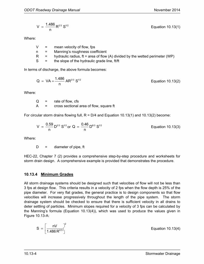
ODOT Roadway Drainage Manual November 2014
10.13-4 Stormwater Drainage
2/3 1/21.486V R S
n= Equation 10.13(1)
Where:
V = mean velocity of flow, fps n = Manning’s roughness coefficient R = hydraulic radius, ft = area of flow (A) divided by the wetted perimeter (WP) S = the slope of the hydraulic grade line, ft/ft
In terms of discharge, the above formula becomes:
2/3 1/21.486Q VA AR S
n= =
Equation 10.13(2)
Where:
Q = rate of flow, cfs A = cross sectional area of flow, square ft
For circular storm drains flowing full, R = D/4 and Equation 10.13(1) and 10.13(2) become:
2/3 1/20.59V D S
n= or
8/3 1/20.46Q D S
n=
Equation 10.13(3)
Where:
D = diameter of pipe, ft HEC-22, Chapter 7 (2) provides a comprehensive step-by-step procedure and worksheets for storm drain design. A comprehensive example is provided that demonstrates the procedure.
10.13.4 Minimum Grades
All storm drainage systems should be designed such that velocities of flow will not be less than 3 fps at design flow. This criteria results in a velocity of 2 fps when the flow depth is 25% of the pipe diameter. For very flat grades, the general practice is to design components so that flow velocities will increase progressively throughout the length of the pipe system. The storm drainage system should be checked to ensure that there is sufficient velocity in all drains to deter settling of particles. Minimum slopes required for a velocity of 3 fps can be calculated by the Manning’s formula (Equation 10.13(4)), which was used to produce the values given in Figure 10.13-A:
2
2/3
nVS
1.486 R
=
Equation 10.13(4)
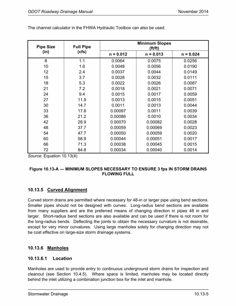
ODOT Roadway Drainage Manual November 2014
Stormwater Drainage 10.13-5
The channel calculator in the FHWA Hydraulic Toolbox can also be used.
Pipe Size (in)
Full Pipe (cfs)
Minimum Slopes (ft/ft)
n = 0.012 n = 0.013 n = 0.024
8 1.1 0.0064 0.0075 0.0256 10 1.6 0.0048 0.0056 0.0190 12 2.4 0.0037 0.0044 0.0149 15 3.7 0.0028 0.0032 0.0111 18 5.3 0.0022 0.0026 0.0087 21 7.2 0.0018 0.0021 0.0071 24 9.4 0.0015 0.0017 0.0059 27 11.9 0.0013 0.0015 0.0051 30 14.7 0.0011 0.0013 0.0044 33 17.8 0.00097 0.0011 0.0039 36 21.2 0.00086 0.0010 0.0034 42 28.9 0.00070 0.00082 0.0028 48 37.7 0.00059 0.00069 0.0023 54 47.7 0.00050 0.00059 0.0020 60 58.9 0.00044 0.00051 0.0017 66 71.3 0.00038 0.00045 0.0015 72 84.8 0.00034 0.00040 0.0014
Source: Equation 10.13(4)
Figure 10.13-A — MINIMUM SLOPES NECESSARY TO ENSURE 3 fps IN STORM DRAINS FLOWING FULL
10.13.5 Curved Alignment
Curved storm drains are permitted where necessary for 48-in or larger pipe using bend sections. Smaller pipes should not be designed with curves. Long-radius bend sections are available from many suppliers and are the preferred means of changing direction in pipes 48 in and larger. Short-radius bend sections are also available and can be used if there is not room for the long-radius bends. Deflecting the joints to obtain the necessary curvature is not desirable, except for very minor curvatures. Using large manholes solely for changing direction may not be cost effective on large-size storm drainage systems.
10.13.6 Manholes
10.13.6.1 Location
Manholes are used to provide entry to continuous underground storm drains for inspection and cleanout (see Section 10.4.5). Where space is limited, manholes may be located directly behind the inlet utilizing a combination junction box for the inlet and manhole.
ODOT Roadway Drainage Manual November 2014
10.13-6 Stormwater Drainage
10.13.6.2 Spacing
The maximum spacing of manholes is as stated in Figure 10.4-A.
10.13.6.3 Sizing
Manholes are usually rectangular or round. The outside diameter of all pipes entering the junction box should fit between the inside faces of the walls.
10.13.6.4 Shaping Inside of Manhole
Proper shaping of manhole invert may reduce eddying and head losses. Figure 10.13-B provides example of efficient manhole shaping.
10.13.7 Sag Point
As discussed in Section 10.5.1, the storm drain that drains a Interstate, freeway and arterial highway sag point should be sized to accommodate the runoff from a 50-year frequency rainfall. This can be accomplished by computing the bypass occurring at the last inlet during a 50-year rainfall. The inlet at the sag point should be designed to accommodate this bypass, and the storm drainage pipe leading from the sag point should be sized to accommodate this additional bypass within the criteria established. To design the pipe leading from the sag point, it may be helpful to convert the additional bypass created by the 50-year rainfall into an equivalent CA that can be added to the design CA.
Some hydraulics designers may want to design separate systems to prevent the above-ground system from draining into the depressed area. This concept may be more costly but, in some cases, may be justified. Another method would be to design the upstream system for a 50-year design to minimize the bypass to the sag point. Each case should be evaluated individually to assess the impacts and risk of flooding a sag point location.
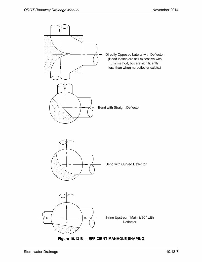
ODOT Roadway Drainage Manual November 2014
Stormwater Drainage 10.13-7
Figure 10.13-B — EFFICIENT MANHOLE SHAPING

ODOT Roadway Drainage Manual November 2014
10.13-8 Stormwater Drainage
ODOT Roadway Drainage Manual November 2014
Stormwater Drainage 10.14-1
10.14 INITIAL SIZE OF PIPE
10.14.1 Introduction
After the preliminary locations of inlets, connecting pipes and outfalls with tailwaters have been determined, the next step is the computation of the rate of discharge to be carried by each reach of the storm drain and the determination of the size and gradient of pipe required to convey this discharge. This is done by starting at the upstream reach, calculating the discharge and sizing the pipe, then proceeding downstream, reach by reach, to the point where the storm drainage system connects with other storm drains or the outfall.
The rate of discharge at any point in the storm drainage system is not necessarily the sum of the inlet flow rates of all inlets above that section of the storm drain. It is generally less than this total. The time of concentration is most influential and, as the time of concentration grows larger, the rainfall intensity to be used in the design grows smaller. In some cases, where a relatively large drainage area with a short time of concentration is added to the system, the peak flow may be larger using the shorter time even though the entire drainage area is not contributing. The prudent hydraulics designer will be alert for unusual conditions and determine which time of concentration controls for each pipe segment. See Section 10.8.5 for a discussion on time of concentration.
For ordinary conditions, storm drainage systems should be sized on the assumption that they will flow full or almost full under the design discharge but will not flow under pressure head. The Manning’s formula is recommended for capacity calculations. The main storm drainage system should be designed by computing the hydraulic grade line and keeping the water surface elevations below the grates or established critical elevations, or both, for the design storm.
10.14.2 Design Procedures
The following procedures are used for the design of storm drainage systems:
Step 1. Determine inlet location, spacing and capacity as outlined in Section 10.12.
Step 2. Prepare the plan layout of the storm drainage system establishing the following design data:
• location of storm drains;
• direction of flow;
• location of manholes/junction boxes (see Section 10.13.6); and
• location of existing utilities (e.g., water, gas, underground cables, existing and proposed foundations).
Step 3. Determine drainage areas, runoff coefficients and a time of concentration to the first inlet. Using an Intensity-Duration-Frequency (IDF) curve, determine the rainfall

ODOT Roadway Drainage Manual November 2014
10.14-2 Stormwater Drainage
intensity. Calculate the discharge with the Rational Method and use the spacing procedure of Section 10.12.10 or locate inlets by ODOT criteria.
Step 4. Size the pipe to convey the discharge by varying the slope and pipe size as necessary. The storm drainage systems are normally designed for full gravity-flow conditions using the design frequency discharges. Initial pipe size and slope can be estimated:
a. using the FHWA Hydraulic Toolbox, Channel Analysis, which contains both circular and rectangular sections; or
b. using the computation procedure provided in the following section.
Step 5. Calculate travel time in the pipe to the next inlet or manhole by dividing pipe length by the velocity. This travel time is added to the time of concentration for a new time of concentration and a new rainfall intensity at the next entry point.
Step 6. Calculate the new area (A) and multiply by the runoff coefficient (C), add to the previous (CA) and multiply by the rainfall intensity (i) to determine the discharge at this inlet. Determine the size of pipe and slope necessary to convey the discharge.
Step 7. Continue this process to the storm drainage outlet.
Step 8. Complete the design by calculating the hydraulic grade line as discussed in Section 10.13.
10.14.3 Storm Sewer Design Procedure
The following hand procedure can be used for simple systems. Instructions are provided for each numbered column in Figure 10.14-A. Software (see Chapter 16 “Hydraulic Software”) is normally used to design and analyze storm drains. If the hydraulics designer designs a storm drain with only a few links or wants to confirm the results of the software calculations, Alternative detailed design procedures and design example are provided in HEC-22 (2).
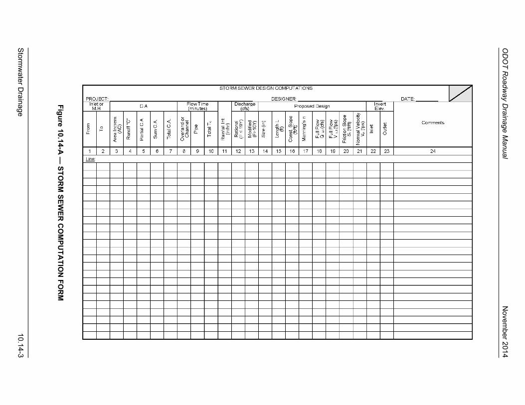
OD
OT
Road
way D
rainage Manual
N
ovem
ber 2014
Storm
water D
rainage 10.14-3
Fig
ure 10.14-A
— S
TO
RM
SE
WE
R C
OM
PU
TA
TIO
N F
OR
M
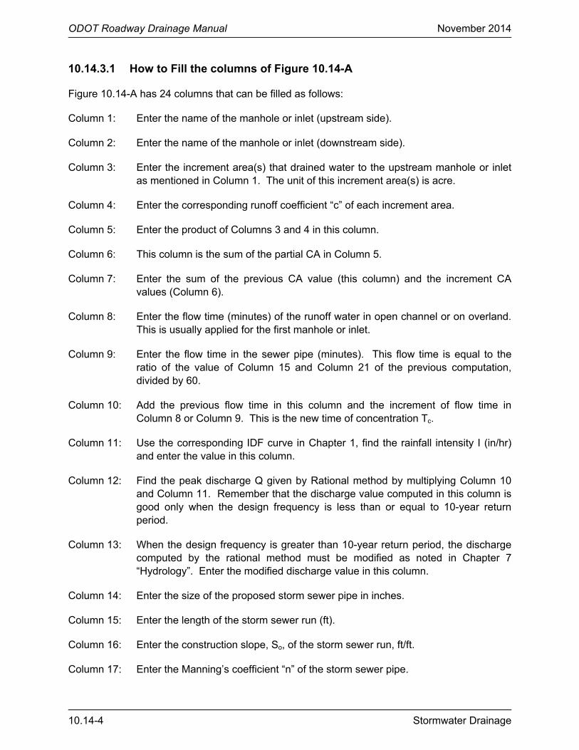
ODOT Roadway Drainage Manual November 2014
10.14-4 Stormwater Drainage
10.14.3.1 How to Fill the columns of Figure 10.14-A
Figure 10.14-A has 24 columns that can be filled as follows:
Column 1: Enter the name of the manhole or inlet (upstream side).
Column 2: Enter the name of the manhole or inlet (downstream side).
Column 3: Enter the increment area(s) that drained water to the upstream manhole or inlet as mentioned in Column 1. The unit of this increment area(s) is acre.
Column 4: Enter the corresponding runoff coefficient “c” of each increment area.
Column 5: Enter the product of Columns 3 and 4 in this column.
Column 6: This column is the sum of the partial CA in Column 5.
Column 7: Enter the sum of the previous CA value (this column) and the increment CA values (Column 6).
Column 8: Enter the flow time (minutes) of the runoff water in open channel or on overland. This is usually applied for the first manhole or inlet.
Column 9: Enter the flow time in the sewer pipe (minutes). This flow time is equal to the ratio of the value of Column 15 and Column 21 of the previous computation, divided by 60.
Column 10: Add the previous flow time in this column and the increment of flow time in Column 8 or Column 9. This is the new time of concentration Tc.
Column 11: Use the corresponding IDF curve in Chapter 1, find the rainfall intensity I (in/hr) and enter the value in this column.
Column 12: Find the peak discharge Q given by Rational method by multiplying Column 10 and Column 11. Remember that the discharge value computed in this column is good only when the design frequency is less than or equal to 10-year return period.
Column 13: When the design frequency is greater than 10-year return period, the discharge computed by the rational method must be modified as noted in Chapter 7 “Hydrology”. Enter the modified discharge value in this column.
Column 14: Enter the size of the proposed storm sewer pipe in inches.
Column 15: Enter the length of the storm sewer run (ft).
Column 16: Enter the construction slope, So, of the storm sewer run, ft/ft.
Column 17: Enter the Manning’s coefficient “n” of the storm sewer pipe.
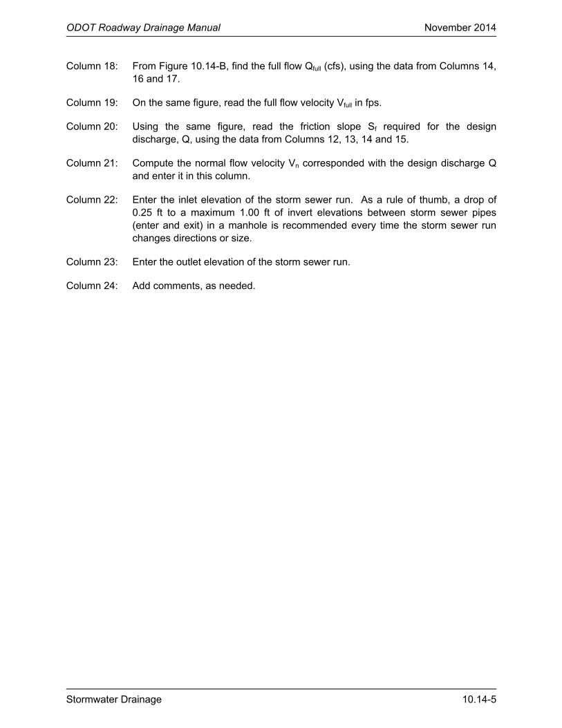
ODOT Roadway Drainage Manual November 2014
Stormwater Drainage 10.14-5
Column 18: From Figure 10.14-B, find the full flow Qfull (cfs), using the data from Columns 14, 16 and 17.
Column 19: On the same figure, read the full flow velocity Vfull in fps.
Column 20: Using the same figure, read the friction slope Sf required for the design discharge, Q, using the data from Columns 12, 13, 14 and 15.
Column 21: Compute the normal flow velocity Vn corresponded with the design discharge Q and enter it in this column.
Column 22: Enter the inlet elevation of the storm sewer run. As a rule of thumb, a drop of 0.25 ft to a maximum 1.00 ft of invert elevations between storm sewer pipes (enter and exit) in a manhole is recommended every time the storm sewer run changes directions or size.
Column 23: Enter the outlet elevation of the storm sewer run.
Column 24: Add comments, as needed.
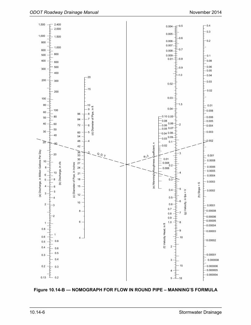
ODOT Roadway Drainage Manual November 2014
10.14-6 Stormwater Drainage
Figure 10.14-B — NOMOGRAPH FOR FLOW IN ROUND PIPE – MANNING’S FORMULA
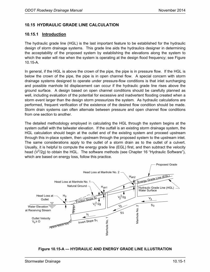
ODOT Roadway Drainage Manual November 2014
Stormwater Drainage 10.15-1
10.15 HYDRAULIC GRADE LINE CALCULATION
10.15.1 Introduction
The hydraulic grade line (HGL) is the last important feature to be established for the hydraulic design of storm drainage systems. This grade line aids the hydraulics designer in determining the acceptability of the proposed system by establishing the elevations along the system to which the water will rise when the system is operating at the design flood frequency; see Figure 10.15-A.
In general, if the HGL is above the crown of the pipe, the pipe is in pressure flow. If the HGL is below the crown of the pipe, the pipe is in open channel flow. A special concern with storm drainage systems designed to operate under pressure-flow conditions is that inlet surcharging and possible manhole lid displacement can occur if the hydraulic grade line rises above the ground surface. A design based on open channel conditions should be carefully planned as well, including evaluation of the potential for excessive and inadvertent flooding created when a storm event larger than the design storm pressurizes the system. As hydraulic calculations are performed, frequent verification of the existence of the desired flow condition should be made. Storm drain systems can often alternate between pressure and open channel flow conditions from one section to another.
The detailed methodology employed in calculating the HGL through the system begins at the system outfall with the tailwater elevation. If the outfall is an existing storm drainage system, the HGL calculation should begin at the outlet end of the existing system and proceed upstream through this in-place system, then upstream through the proposed system to the upstream inlet. The same considerations apply to the outlet of a storm drain as to the outlet of a culvert. Usually, it is helpful to compute the energy grade line (EGL) first, and then subtract the velocity head (V2/2g) to obtain the HGL. The software methods (see Chapter 16 “Hydraulic Software”), which are based on energy loss, follow this practice.
Figure 10.15-A — HYDRAULIC AND ENERGY GRADE LINE ILLUSTRATION

ODOT Roadway Drainage Manual November 2014
10.15-2 Stormwater Drainage
10.15.2 ODOT Practice (HGL)
The following section provides guidelines for establishing DOT hydraulic grade line (HGL) practice.
Computation of the hydraulic grade line of a storm drainage run will not be necessary where:
• the slope and the pipe sizes are chosen so that the slope is equal to or greater than the friction slope,
• the top surfaces of successive pipes are aligned at changes in size (rather than flow lines being aligned), and
• the surface of the water at the point of discharge does not rise above the top of the outlet.
The pipe will not operate under pressure in these cases, and the slope of the water surface under capacity discharge will approximately parallel the slope of the pipe invert.
However, where different sized pipe inverts are placed on the same grade, causing the smaller pipe to discharge against head, or when it is desired to check the storm drainage system against larger-than-design floods, it will be necessary to compute the hydraulic grade line of the entire storm drainage system. Begin with the tailwater elevation at the storm drainage outfall and progress upward through the entire length of the storm drain. For every run, compute the friction loss and plot the elevation of the total head at each manhole and inlet using the procedures in Section 10.15.2.
The methodology in HEC-22 (2) can be used for the calculation of the energy losses for a storm drainage system. The method is summarized in Section 10.13. See HEC-22 Chapter 7 (2) for symbol definitions, design procedures, computation sheets and an example calculation. See Chapter 16 “Hydraulic Software” for software for the storm drainage analysis, which includes the HGL.
If the hydraulic grade line does not rise above the top of any manhole or above an inlet entrance, the storm drainage system is satisfactory. If the HGL rises above these points, blowouts will occur through manholes and inlets. Pipe sizes or gradients can be increased as necessary to eliminate such blowouts. Standard practice is to ensure that the HGL is below the top of the inlet for the design discharge (some states add an additional safety factor that can be up to 12 in).
10.15.3 Tailwater
For most design applications where the flow is subcritical, the tailwater will either be above the crown of the outlet or can be considered to be between the crown and critical depth. To determine the EGL, begin with the tailwater elevation or (dc + D)/2, whichever is higher, add the velocity head for full flow and proceed upstream to adding appropriate losses (e.g., exit, friction, junction, bend, entrance).
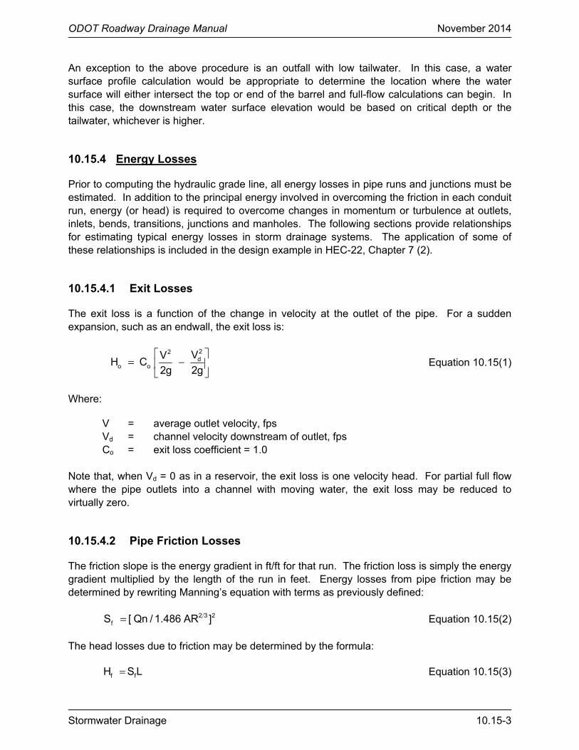
ODOT Roadway Drainage Manual November 2014
Stormwater Drainage 10.15-3
An exception to the above procedure is an outfall with low tailwater. In this case, a water surface profile calculation would be appropriate to determine the location where the water surface will either intersect the top or end of the barrel and full-flow calculations can begin. In this case, the downstream water surface elevation would be based on critical depth or the tailwater, whichever is higher.
10.15.4 Energy Losses
Prior to computing the hydraulic grade line, all energy losses in pipe runs and junctions must be estimated. In addition to the principal energy involved in overcoming the friction in each conduit run, energy (or head) is required to overcome changes in momentum or turbulence at outlets, inlets, bends, transitions, junctions and manholes. The following sections provide relationships for estimating typical energy losses in storm drainage systems. The application of some of these relationships is included in the design example in HEC-22, Chapter 7 (2).
10.15.4.1 Exit Losses
The exit loss is a function of the change in velocity at the outlet of the pipe. For a sudden expansion, such as an endwall, the exit loss is:
22d
o o
VVH C
2g 2g
= −
Equation 10.15(1)
Where:
V = average outlet velocity, fps Vd = channel velocity downstream of outlet, fps Co = exit loss coefficient = 1.0
Note that, when Vd = 0 as in a reservoir, the exit loss is one velocity head. For partial full flow where the pipe outlets into a channel with moving water, the exit loss may be reduced to virtually zero.
10.15.4.2 Pipe Friction Losses
The friction slope is the energy gradient in ft/ft for that run. The friction loss is simply the energy gradient multiplied by the length of the run in feet. Energy losses from pipe friction may be determined by rewriting Manning’s equation with terms as previously defined:
2 3 2fS [ Qn / 1.486 AR ]= Equation 10.15(2)
The head losses due to friction may be determined by the formula:
f fH S L= Equation 10.15(3)
ODOT Roadway Drainage Manual November 2014
10.15-4 Stormwater Drainage
Manning’s equation can also be written to determine friction losses for storm drains as follows:
2
f 2.67
QnH L
0.46D =
(circular shapes) Equation 10.15(4)
2 2
f 4/3
29 n L VH
2gR
=
Equation 10.15(5)
Where:
Hf = total head loss due to friction, ft n = Manning’s roughness coefficient D = diameter of pipe, ft L = length of pipe, ft V = mean velocity, fps R = hydraulic radius, ft g = 32.2 ft/s2 Sf = slope of hydraulic grade line, ft/ft
10.15.4.3 Bend Losses
The bend loss coefficient for storm drainage system design is minor but can be evaluated using the formula:
( ) ( )2b oh 0.0033 V / 2g= Δ Equation 10.15(6)
Where:
Δ = angle of curvature, degrees
10.15.4.4 Manhole/Inlet Losses Inlet
The head loss encountered from one pipe to another through a manhole is commonly represented as being proportional to the velocity head at the outlet pipe. Using KM to signify this constant of proportionality, the energy loss is:
2
M M
VH K
2g
=
Equation 10.15(7)
For simple systems, an estimate or approximation of the KM value can be used. For complex systems with complicated junctions, the KM value should be determined using the HEC-22 (2) method.
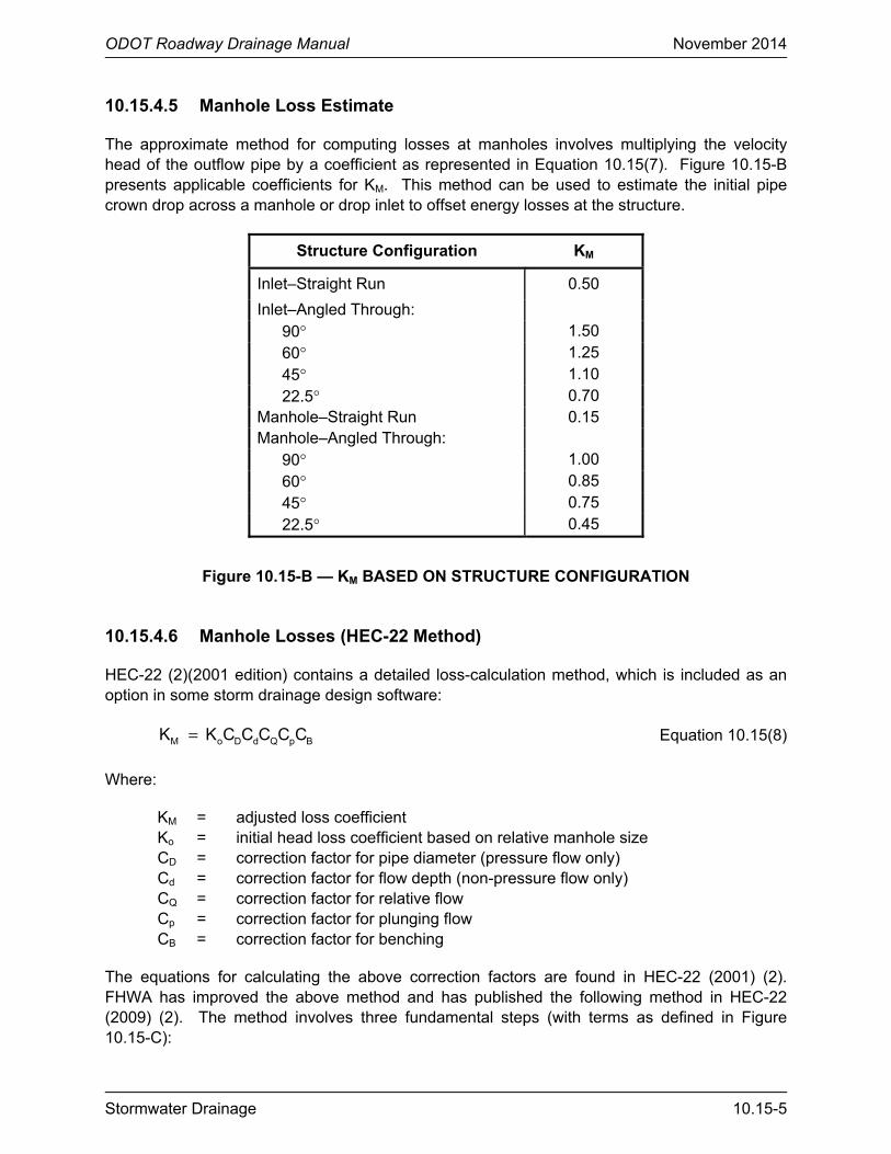
ODOT Roadway Drainage Manual November 2014
Stormwater Drainage 10.15-5
10.15.4.5 Manhole Loss Estimate
The approximate method for computing losses at manholes involves multiplying the velocity head of the outflow pipe by a coefficient as represented in Equation 10.15(7). Figure 10.15-B presents applicable coefficients for KM. This method can be used to estimate the initial pipe crown drop across a manhole or drop inlet to offset energy losses at the structure.
Structure Configuration KM
Inlet–Straight Run 0.50
Inlet–Angled Through: 90° 1.50 60° 1.25 45° 1.10 22.5° 0.70
Manhole–Straight Run 0.15 Manhole–Angled Through:
90° 1.00 60° 0.85 45° 0.75 22.5° 0.45
Figure 10.15-B — KM BASED ON STRUCTURE CONFIGURATION 10.15.4.6 Manhole Losses (HEC-22 Method)
HEC-22 (2)(2001 edition) contains a detailed loss-calculation method, which is included as an option in some storm drainage design software:
M o D d Q p BK K C C C C C= Equation 10.15(8)
Where:
KM = adjusted loss coefficient Ko = initial head loss coefficient based on relative manhole size CD = correction factor for pipe diameter (pressure flow only) Cd = correction factor for flow depth (non-pressure flow only) CQ = correction factor for relative flow Cp = correction factor for plunging flow CB = correction factor for benching
The equations for calculating the above correction factors are found in HEC-22 (2001) (2). FHWA has improved the above method and has published the following method in HEC-22 (2009) (2). The method involves three fundamental steps (with terms as defined in Figure 10.15-C):

ODOT Roadway Drainage Manual November 2014
10.15-6 Stormwater Drainage
Step 1. Determine an initial manhole energy level (Eai) based on inlet control (weir and orifice) or outlet control (partial and full flow) equations.
Step 2. Adjust the initial manhole energy level based on benching, inflow angle(s) and plunging flows to compute the final calculated energy level (Ea).
Step 3. Calculate the exit loss from each inflow pipe and estimate the energy gradeline (EGL), which will then be used to continue calculations upstream.
Figure 10.15-C — DEFINITION SKETCH FOR HEC-22 (2009) MANHOLE LOSS METHOD 10.15.4.7 ODOT Manhole Loss Method
The following general types of manhole losses can occur in either open channel flow or full barrel flow:
10.15.4.7.1 Terminal Manhole Losses
A manhole is called terminal manhole when it has only outflow pipe. This manhole receives the runoff water directly through gutter inlets. The head loss Ht through a terminal manhole is computed by the following formula:
g2
VH
2o
t = Equation 10.15(9)
Where: Ht = Head loss at terminal, ft Vo = Flow velocity in outflow pipe, fps g = Specific gravity = 32.2 ft/s2
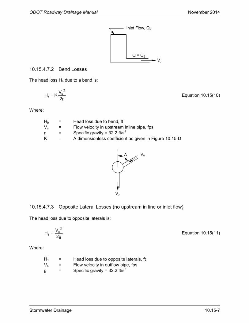
ODOT Roadway Drainage Manual November 2014
Stormwater Drainage 10.15-7
10.15.4.7.2 Bend Losses
The head loss Hb due to a bend is:
g2
VKH
2u
b = Equation 10.15(10)
Where: Hb = Head loss due to bend, ft Vu = Flow velocity in upstream inline pipe, fps g = Specific gravity = 32.2 ft/s2 K = A dimensionless coefficient as given in Figure 10.15-D 10.15.4.7.3 Opposite Lateral Losses (no upstream in line or inlet flow)
The head loss due to opposite laterals is:
g2
VH
2o
1 = Equation 10.15(11)
Where: H1 = Head loss due to opposite laterals, ft Vo = Flow velocity in outflow pipe, fps g = Specific gravity = 32.2 ft/s2

ODOT Roadway Drainage Manual November 2014
10.15-8 Stormwater Drainage
10.15.4.7.4 Junction Losses (with or without inlet flow)
The head losses due to the convergence of several storm sewer pipes in a manhole are:
g2
V)Q/Q)(K1(
g2
V)Q/Q)(K1(
g2
V)Q/Q(
g2
VH
2r
orr
21
o11
2u
ou
2o
j −−−−−= Equation 10.15(12)
Where:
Hj = Head loss in the manhole, ft Vo = Flow velocity in outflow pipe, fps Vu = Flow velocity in upstream inflow pipe, fps Vr = Flow velocity in right lateral pipe, fps V1 = Flow velocity in left lateral pipe, fps g = Specific gravity = 32.2 ft/s2 K1 = Bend coefficient, left lateral – see Figure 10.15-D Kr = Bend coefficient, right lateral – see Figure 10.15-D
The total head losses in the manhole for open channel flow are:
H = Ht + Hb + H1 + Hj Equation 10.15(13)
Where:
H = Total head losses, ft Ht, Hb, H1, Hj = Same as defined above, ft
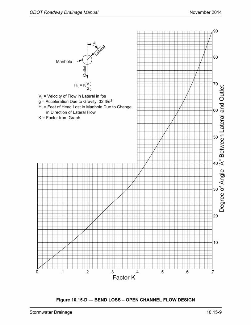
ODOT Roadway Drainage Manual November 2014
Stormwater Drainage 10.15-9
Figure 10.15-D — BEND LOSS – OPEN CHANNEL FLOW DESIGN
ODOT Roadway Drainage Manual November 2014
10.15-10 Stormwater Drainage
10.15.5 Hydraulic Grade Line Design Procedure
The following hand procedure can be used for simple systems. Instructions are provided for each numbered column in Figure 10.15-M. Software (see Chapter 16 “Hydraulic Software”) is normally used to design and analyze storm drains. If the hydraulics designer designs a storm drain with only a few links or wants to confirm the results of the software calculations. The equations and charts necessary to manually calculate the location of the hydraulic grade line are included in HEC-22 (2) and are illustrated with an example problem. HEC-22 contains a computation form that permits the use of the approximate KM and an additional form for documenting the HEC-22 (2009) loss method.
Figure 10.15-M (hydraulic grade line computations) has 32 columns that can be filled as follows:
Column 1: Enter the name of the manhole, inlet or outflow in consideration.
Column 2: Enter the station of the manhole, inlet or outflow in consideration.
Column 3: Enter the downstream invert elevation of the manhole, inlet or outflow as mentioned in Column 1. The terms upstream or downstream are referred to the direction of the flow.
Column 4: Enter the discharge, Qo, (cfs) that leaves the inlet or manhole as mentioned in Column 1.
Column 5: Enter the diameter, Do, (in) of the downstream side pipe.
Column 6: Enter the construction slope, So, of the downstream side pipe.
Column 7: Enter the flow depth in the downstream pipe (ft). This flow depth is not necessarily equal to the flow normal depth Dn.
Column 8: Explain in this column where the flow depth in Column 7 comes from (backwater, drawdown, full flow, normal depth).
Column 9: Enter the flow velocity corresponded to the flow depth of Column 7 in fps.
Column 10: Enter the downstream velocity head (ft) in this column.
Column 11: Enter the hydraulic gradeline (H.G.) elevation at the downstream side of the inlet or manhole. This H.G. elevation can either be given or by adding Columns 3 and 7.
Column 12: Enter the energy gradeline (E.G.) elevation at the downstream side of the inlet or manhole. This E.G. elevation is the sum of Columns 10 and 11.
Column 13: Enter the head loss due to bend. For open channel flow, use Figure 10.15-D and Equation 10.15(10). For pressured flow, use Figure 10.15-E.
Column 14: Enter the head loss due to opposed laterals. Use Equation 10.15(11) for open channel flow and Figures 10.15-F and 10.15-G for pressured flow.

ODOT Roadway Drainage Manual November 2014
Stormwater Drainage 10.15-11
Column 15: Enter the head loss due to terminal inlet or manhole. Use Equation 10.15(9) for open channel flow and Figures 10.15-H for pressured flow.
Column 16: Enter the head loss in a junction where several storm sewer pipes converged. Use Equation 10.15(12) for open channel flow and Figures 10.15-I, 10.15-J and 10.15-K for pressured flow.
Column 17: Enter total head losses that is the sum of Columns 13, 14, 15 and 16.
Column 18: Enter the upstream invert elevation of the manhole, inlet or outflow as mentioned in Column 1. The terms upstream or downstream are referred to the direction of the flow.
Column 19: Enter the energy gradeline elevation at the upstream side of the inlet or manhole. This E.G. line is the sum of Columns 12 and 17.
Column 20: Enter the discharge Qu (cfs) of the upstream side pipe (on the truck line) that enters the manhole or junction.
Column 21: Enter the upstream pipe diameter, Du (in).
Column 22: Enter the construction slope, So, of that upstream pipe in ft/ft.
Column 23: Enter the friction slope, Sf, of the upstream pipe in ft/ft. This friction slope can be read directly from Figure 10.14-A or can be computed from Figure 10.14-B, using the data from Columns 19 and 20.
Column 24: Enter the length of the upstream pipe in feet. It can be read directly from Column 15 of Figure 10.14-A.
Column 25: Enter the flow depth, du, in the upstream pipe (ft). This flow depth is not necessarily equal to the flow normal depth Dn.
Column 26: Explain in this column where the flow depth in Column 25 comes from backwater, drawdown, full flow, or normal depth.
Column 27: Enter the flow velocity, Vu, corresponded to the flow depth of Column 25 in fps.
Column 28: Enter the upstream velocity head (ft) in this column.
Column 29: Enter the friction loss, Hf, in the upstream pipe (ft).
• For full or pressured flow, this friction loss Hf is equal to the product of Columns 23 and 24.
• For open chanel flow, this friction loss Hf is computed by subtracting Column 19 from Column 12.

ODOT Roadway Drainage Manual November 2014
10.15-12 Stormwater Drainage
Column 30: Enter the hydraulic gradeline elevation at the upstream side of the inlet or manhole. This H.G. elevation is computed by subtracting Column 28 from Column 19.
Column 31: Enter the elevation of the top of this manhole or inlet, ft.
Column 32: Enter the clearance (feet) between top of the manhole (or inlet) and the upstream H.G. elevation. It is computed by subtracting Column 30 from Column 31.
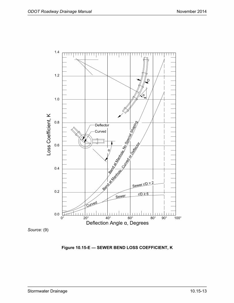
ODOT Roadway Drainage Manual November 2014
Stormwater Drainage 10.15-13
Source: (9)
Figure 10.15-E — SEWER BEND LOSS COEFFICIENT, K
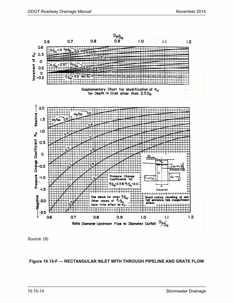
ODOT Roadway Drainage Manual November 2014
10.15-14 Stormwater Drainage
Source: (9)
Figure 10.15-F — RECTANGULAR INLET WITH THROUGH PIPELINE AND GRATE FLOW
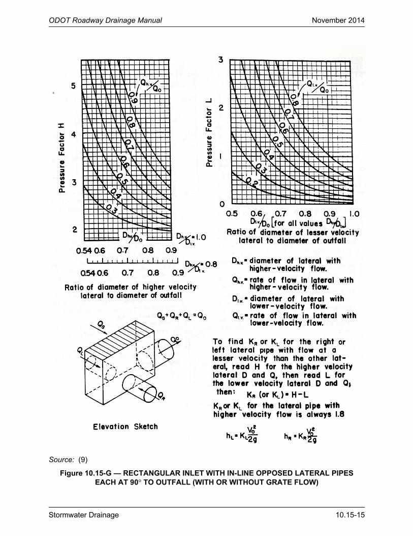
ODOT Roadway Drainage Manual November 2014
Stormwater Drainage 10.15-15
Source: (9)
Figure 10.15-G — RECTANGULAR INLET WITH IN-LINE OPPOSED LATERAL PIPES EACH AT 90° TO OUTFALL (WITH OR WITHOUT GRATE FLOW)
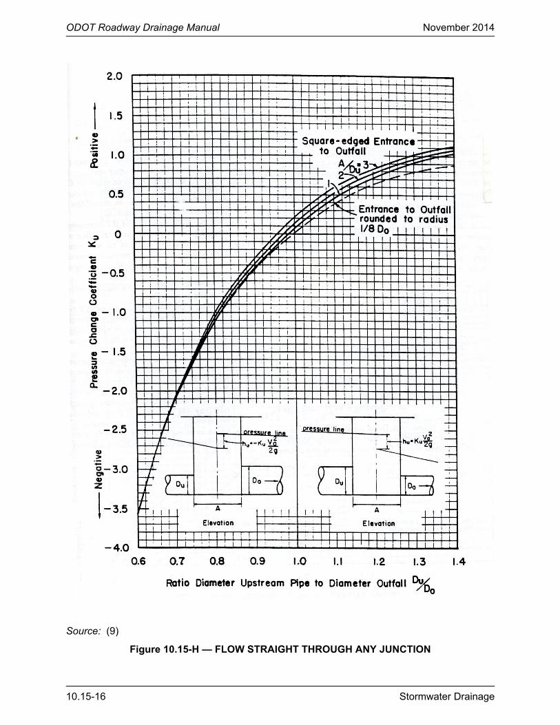
ODOT Roadway Drainage Manual November 2014
10.15-16 Stormwater Drainage
Source: (9)
Figure 10.15-H — FLOW STRAIGHT THROUGH ANY JUNCTION
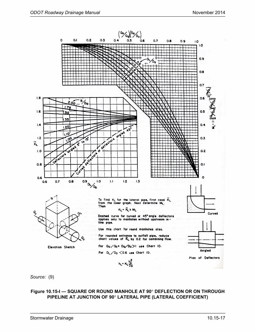
ODOT Roadway Drainage Manual November 2014
Stormwater Drainage 10.15-17
Source: (9)
Figure 10.15-I — SQUARE OR ROUND MANHOLE AT 90° DEFLECTION OR ON THROUGH PIPELINE AT JUNCTION OF 90° LATERAL PIPE (LATERAL COEFFICIENT)
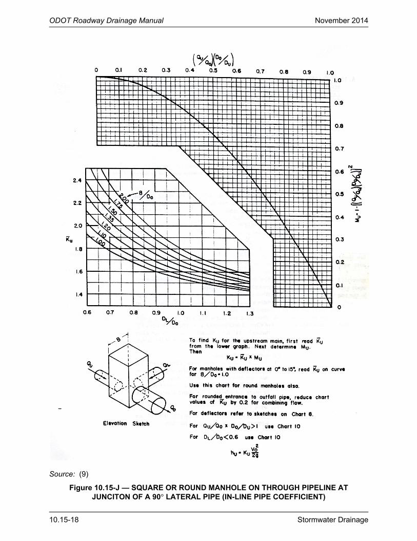
ODOT Roadway Drainage Manual November 2014
10.15-18 Stormwater Drainage
Source: (9)
Figure 10.15-J — SQUARE OR ROUND MANHOLE ON THROUGH PIPELINE AT JUNCITON OF A 90° LATERAL PIPE (IN-LINE PIPE COEFFICIENT)
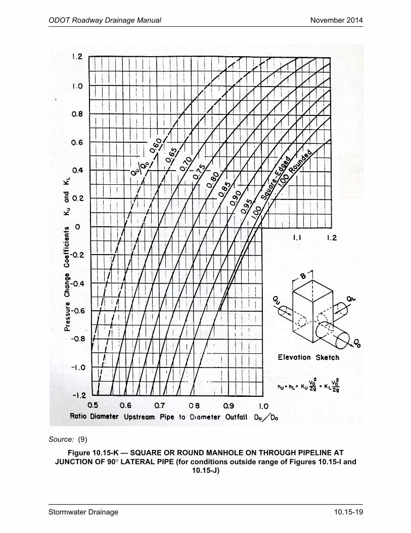
ODOT Roadway Drainage Manual November 2014
Stormwater Drainage 10.15-19
Source: (9)
Figure 10.15-K — SQUARE OR ROUND MANHOLE ON THROUGH PIPELINE AT JUNCTION OF 90° LATERAL PIPE (for conditions outside range of Figures 10.15-I and
10.15-J)
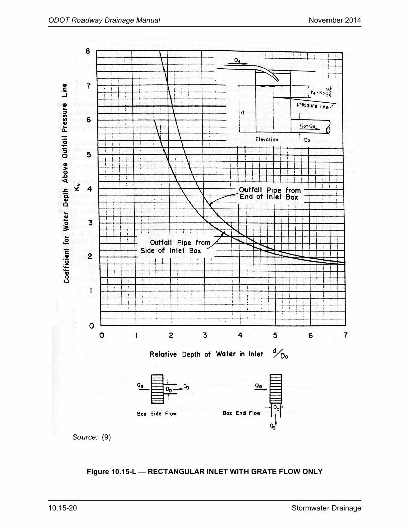
ODOT Roadway Drainage Manual November 2014
10.15-20 Stormwater Drainage
Source: (9)
Figure 10.15-L — RECTANGULAR INLET WITH GRATE FLOW ONLY
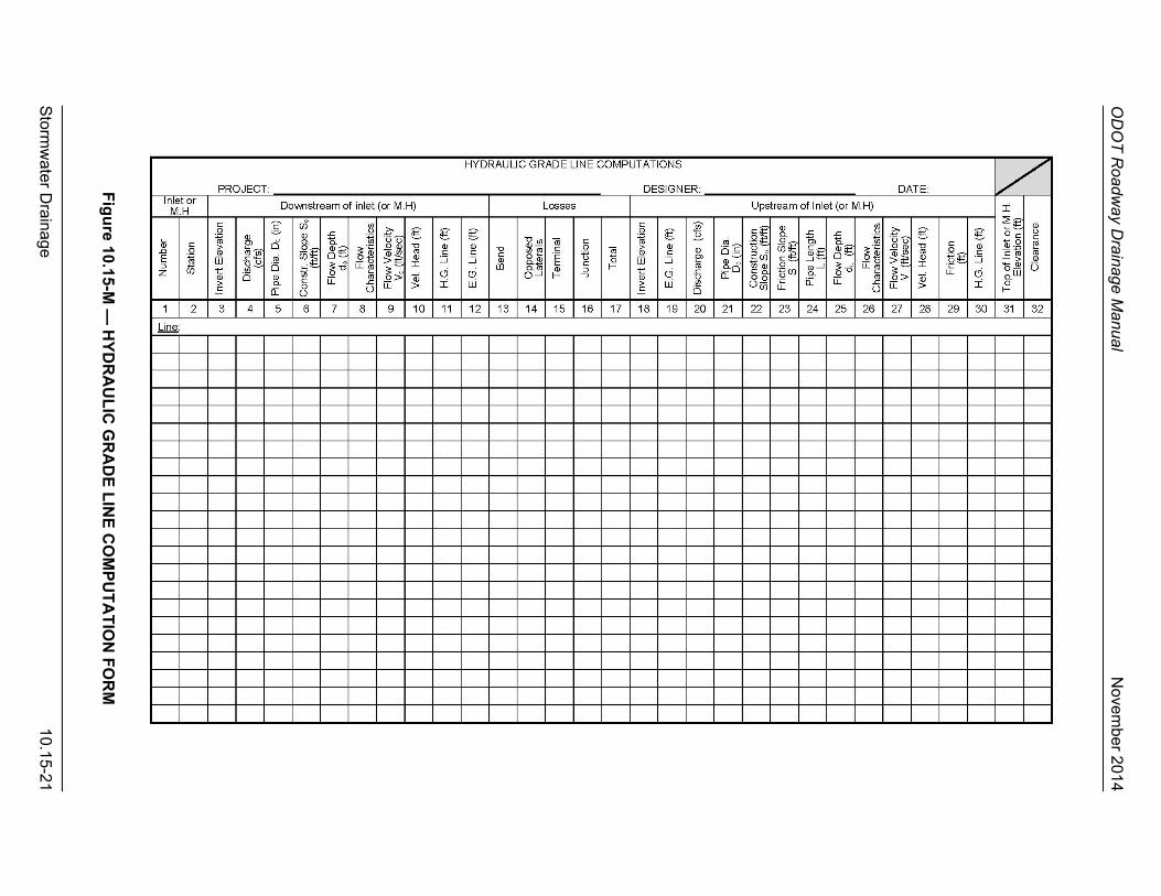
OD
OT
Road
way D
rainage Manual
N
ovem
ber 2014
Storm
water D
rainage 10.15-21
Fig
ure 10.15-M
— H
YD
RA
UL
IC G
RA
DE
LIN
E C
OM
PU
TA
TIO
N F
OR
M

ODOT Roadway Drainage Manual November 2014
10.15-22 Stormwater Drainage

ODOT Roadway Drainage Manual November 2014
Stormwater Drainage 10.16-1
10.16 ODOT DESIGN EXAMPLE
10.16.1 Layout and Data
Given: Figure 10.16-A shows a hypothetical layout of a storm sewer system for an urban depressed highway which is located in Oklahoma hydrological zone number 2.
All sub-basins characteristics (e.g., area, runoff, coefficient) are given as shown.
Required:
From this given information, design the characteristics (e.g., pipe size, construction slope, Manning’s n) of the storm sewer system to drain the runoff to Blue Creek, assuming:
1. The water elevation in the Blue Creek corresponded with a flood of 50-year frequency is at elevation 96.00, or
2. The water elevation in the Blue Creek corresponded with a flood of 50-year frequency is at elevation 98.60.
Typically, only one water elevation is associated with a 50-year frequency. The second water elevation (98.60) is included to illustrate the Hydraulics Grade line computation procedure.
Solution: From Section 10.5.1, the recommended design frequency for a storm sewer system located in a sag (depressed) is 50-year return period.
From Figure 10.16-A, the proposed storm sewer consists of seven lines: A, B, C, D, E and F.
For the simplicity of the example, only the design of Line “A” (including inlets 1, 2 and manholes MH1, MH2, MH3, MH4 and MH5 to outfall) of the proposed storm sewer system will be presented below. The design of the other lines will be computed in the same manner.
The ground profile of Line “A” is as shown in Figure 10.16-B.
The preliminary design of Line “A” of the proposed storm sewer system will start from upstream (Inlet 1) and proceed downward to outflow at Blue Creek, using Figure 10.16-A.
A summary of this preliminary design is as shown in Figure 10.16-C and the profile of Line “A” of the proposed storm sewer system is as shown in Figure 10.16-D.
The next step is to check if the preliminary design of the storm sewer system is satisfied with the design criteria (Section 10.5).
Step 1. The 50-year flood water elevation in Blue Creek is at El. 96.00. The depth of the tailwater at the outfall is:
96.00 – 95.00 = 1.00 ft
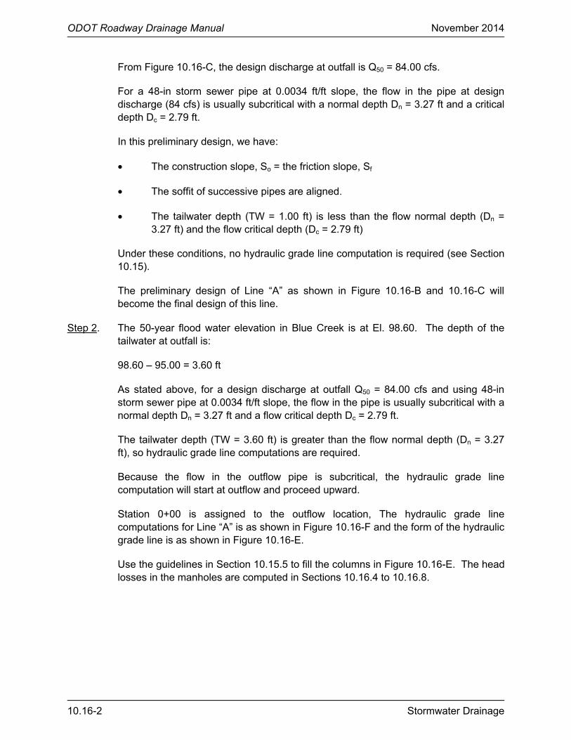
ODOT Roadway Drainage Manual November 2014
10.16-2 Stormwater Drainage
From Figure 10.16-C, the design discharge at outfall is Q50 = 84.00 cfs.
For a 48-in storm sewer pipe at 0.0034 ft/ft slope, the flow in the pipe at design discharge (84 cfs) is usually subcritical with a normal depth Dn = 3.27 ft and a critical depth Dc = 2.79 ft.
In this preliminary design, we have:
• The construction slope, So = the friction slope, Sf
• The soffit of successive pipes are aligned.
• The tailwater depth (TW = 1.00 ft) is less than the flow normal depth (Dn = 3.27 ft) and the flow critical depth (Dc = 2.79 ft)
Under these conditions, no hydraulic grade line computation is required (see Section 10.15).
The preliminary design of Line “A” as shown in Figure 10.16-B and 10.16-C will become the final design of this line.
Step 2. The 50-year flood water elevation in Blue Creek is at El. 98.60. The depth of the tailwater at outfall is:
98.60 – 95.00 = 3.60 ft
As stated above, for a design discharge at outfall Q50 = 84.00 cfs and using 48-in storm sewer pipe at 0.0034 ft/ft slope, the flow in the pipe is usually subcritical with a normal depth Dn = 3.27 ft and a flow critical depth Dc = 2.79 ft.
The tailwater depth (TW = 3.60 ft) is greater than the flow normal depth (Dn = 3.27 ft), so hydraulic grade line computations are required.
Because the flow in the outflow pipe is subcritical, the hydraulic grade line computation will start at outflow and proceed upward.
Station 0+00 is assigned to the outflow location, The hydraulic grade line computations for Line “A” is as shown in Figure 10.16-F and the form of the hydraulic grade line is as shown in Figure 10.16-E.
Use the guidelines in Section 10.15.5 to fill the columns in Figure 10.16-E. The head losses in the manholes are computed in Sections 10.16.4 to 10.16.8.
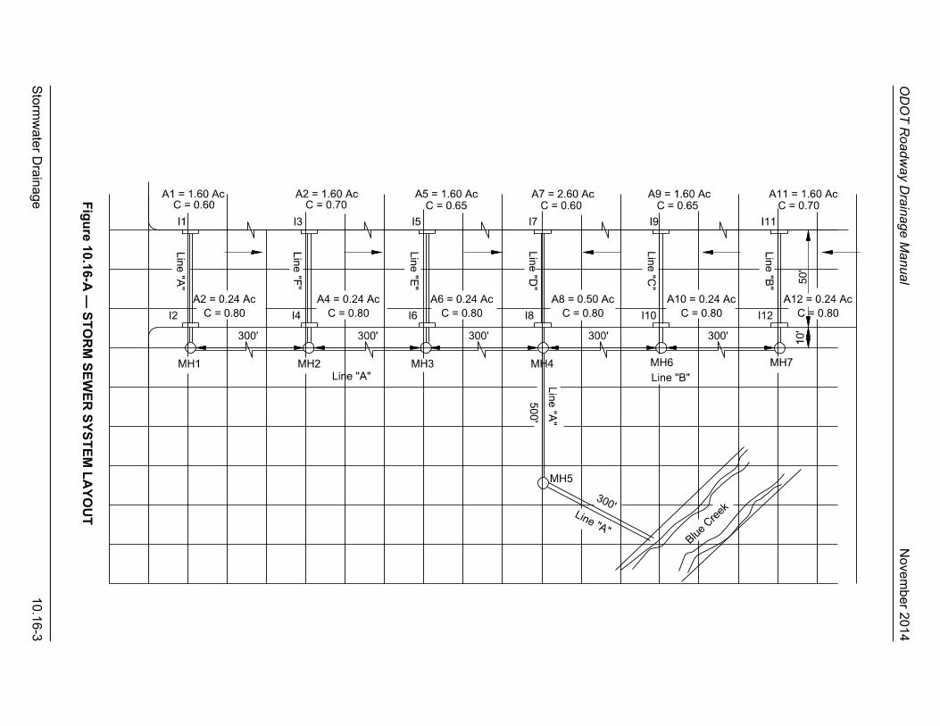
OD
OT
Road
way D
rainage Manual
N
ovem
ber 2014
Storm
water D
rainage 10.16-3
Fig
ure 10.16-A
— S
TO
RM
SE
WE
R S
YS
TE
M L
AY
OU
T
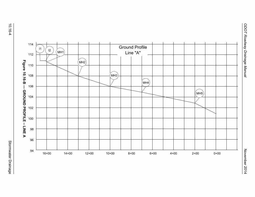
OD
OT
Road
way D
rainage Manual
N
ovem
ber 2014
10.16-4 S
tormw
ater Drainage
Fig
ure 10.16-B
— G
RO
UN
D P
RO
FIL
E – L
INE
A
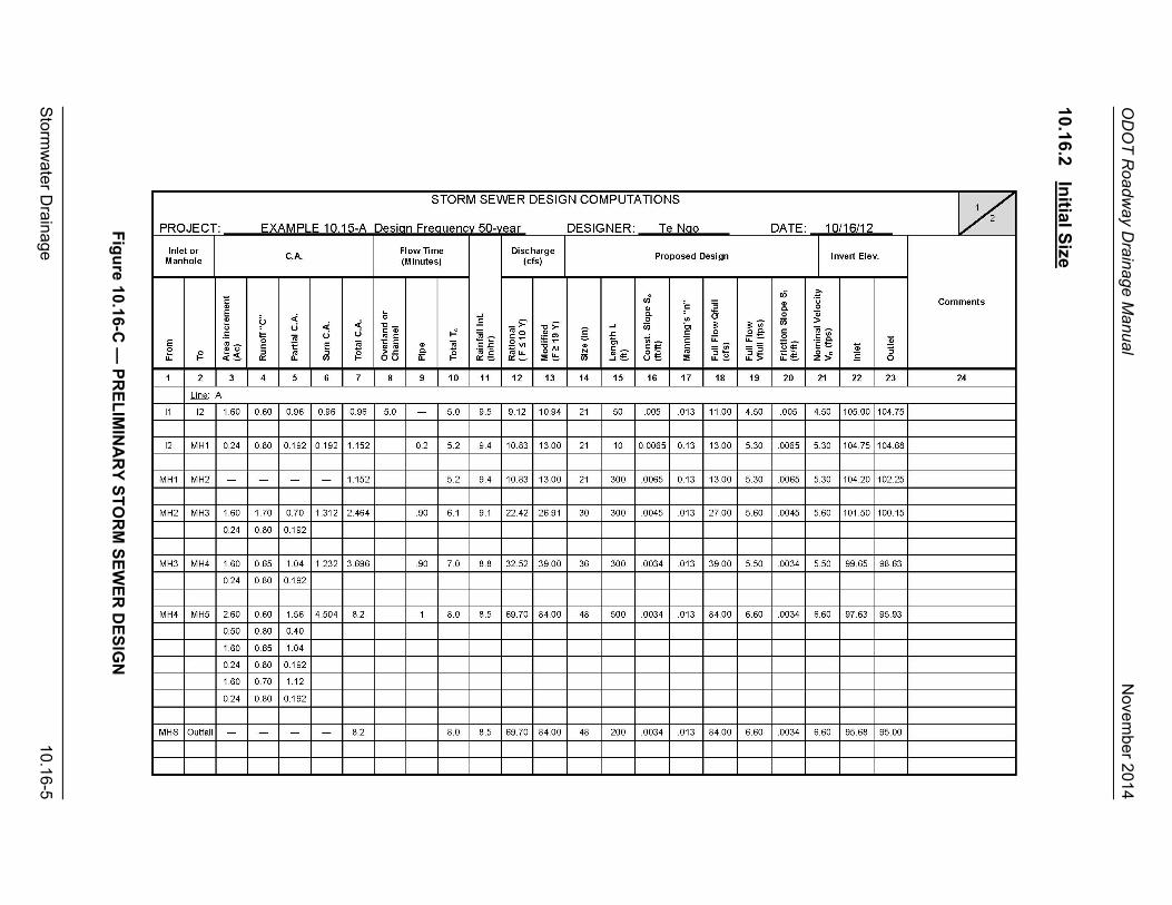
OD
OT
Road
way D
rainage Manual
N
ovem
ber 2014
Storm
water D
rainage 10.16-5
10.16.2 In
itial Size
Fig
ure 10.16-C
— P
RE
LIM
INA
RY
ST
OR
M S
EW
ER
DE
SIG
N
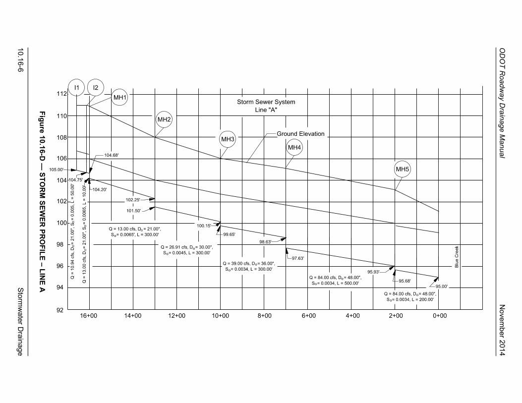
OD
OT
Road
way D
rainage Manual
N
ovem
ber 2014
10.16-6 S
tormw
ater Drainage
Fig
ure 10.16-D
— S
TO
RM
SE
WE
R P
RO
FIL
E –
LIN
E A
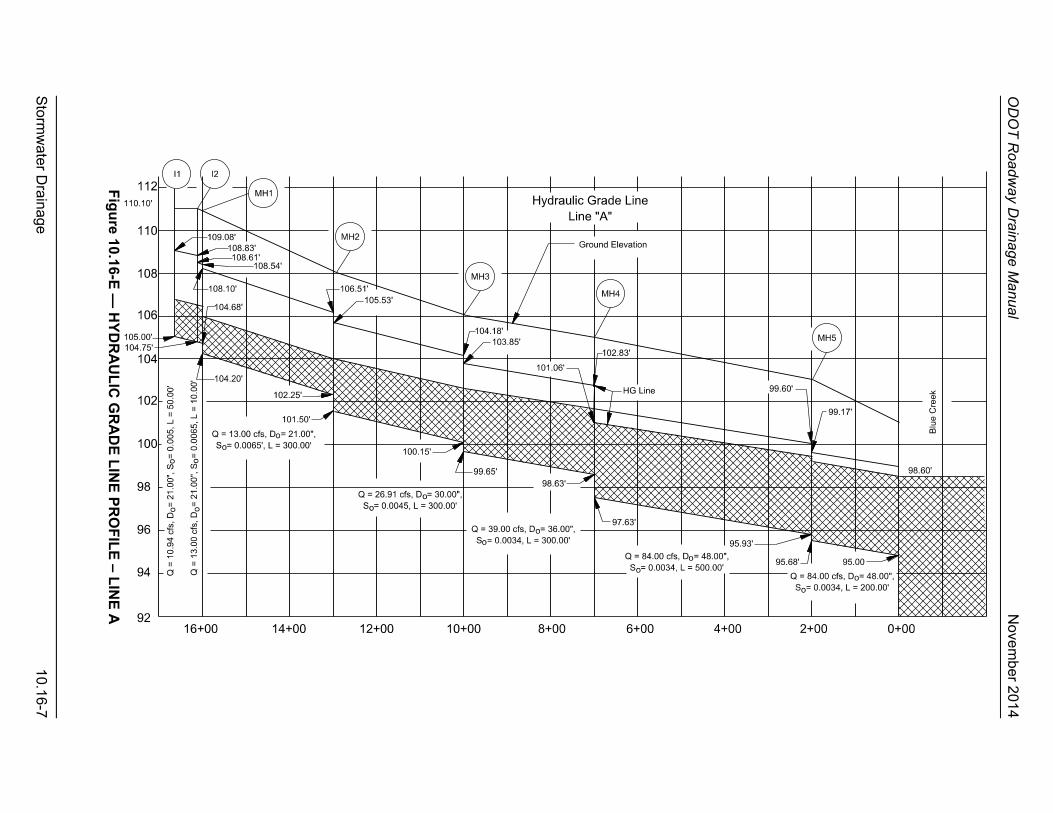
OD
OT
Road
way D
rainage Manual
N
ovem
ber 2014
Storm
water D
rainage 10.16-7
Fig
ure 10.16-E
— H
YD
RA
UL
IC G
RA
DE
LIN
E P
RO
FIL
E – L
INE
A
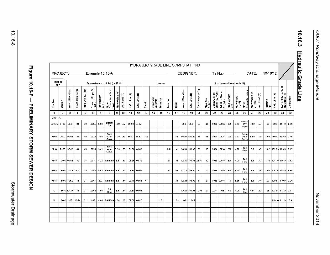
OD
OT
Road
way D
rainage Manual
N
ovem
ber 2014
10.16-8 S
tormw
ater Drainage
10.16.3 H
ydrau
lic Grad
e Lin
e
Fig
ure 10.16-F
— P
RE
LIM
INA
RY
ST
OR
M S
EW
ER
DE
SIG
N

ODOT Roadway Drainage Manual November 2014
Stormwater Drainage 10.16-9
10.16.4 Manhole MH5
Manhole MH5 is located 200 ft upstream of the outflow and is assumed to be a reinforced concrete round manhole with 6 ft inside diameter. The characteristics of the pipes that enter and exit the manhole and the manhole loss are as follows:
A. Downstream (Exit) end of manhole MH5
- Discharge Qo = 84 cfs (Column 13, Figure 10.16-C) - Pipe diameter = 48 in (Column 14, Figure10.16-C) - Construction slope, So
= 0.0034 ft/ft (Column 16, Figure 10.16-C) - Invert elevation = El. 95.68 - Flow depth = 3.49 ft (from backwater curve computation) - Flow velocity Vo = 7.19 fps - Velocity head = (Vo x Vo)/2g = 0.80 - H.G. line elevation = 95.68 + 3.49 = El. 99.17 - E.G. line elevation = 99.17 + 0.8 = El. 99.97
B. Upstream (Entrance) end of manhole MH5
The upstream pipe characteristics are: - Discharge Qu = 84 cfs (Column 13, Figure 10.16-C) - Pipe diameter = 48 in (Column 14, Figure 10.16-C) - Construction slope, So
= 0.0034 ft/ft (Column 16, Figure 10.16-C) - Invert elevation = El. 95.93 (Column 23, Figure 10.16-C)
C. Head loss in manhole MH5
The head loss in manhole MH5 consists of only the loss due to the 67° bend.
From the data given above, the flow depth at downstream side of MH5 is 3.49 ft, which is less than the pipe diameter, therefore, we have open channel flow in the pipe downstream of MH5.

ODOT Roadway Drainage Manual November 2014
10.16-10 Stormwater Drainage
Now assume that the flow in the pipe upstream of MH5 is operated as open channel flow too. The manhole loss in MH5 then can be computed by Equation 10.15(6) with the coefficient K read directly from Figure 10.15-D (open channel flow).
For a 67° bend, K = 0.60 and the head loss in manhole MH5 is:
Hb = K x ((Vo x Vo) /2g) = 0.6 x 0.8 = 0.48 ft
The E.G. line elevation at upstream side of manhole MH5 then becomes:
E.G. line elevation = 99.87 + 0.48 = El. 100.35
The specific energy at the upstream of manhole MH5 is:
Specific energy = 100.35 – 95.93 = 4.42 ft
In order to have the specific energy = 4.42 ft, the flow depth in the 48-in upstream pipe must be (by trial and error method):
• Flow depth = 3.67 ft
• Flow velocity Vu = 6.96 fps
• Velocity head = (Vu x Vu) / 2g = 0.75 ft
From the computation above, the upstream flow depth is 3.67 ft, which is less than the pipe diameter, therefore, the flow in the upstream pipe is open channel flow and our assumption is correct.
The H.G. line elevation at upstream side of manhole MH5 is:
H.G. line elevation = E.G. line elevation – Velocity head = 100.35 – 0.75 = El. 99.60
D. H.G. line elevation check
From Figure 10.16-D, the elevation at the top of manhole MH5 is at El. 103.0 or about 3.4 ft higher than the highest H.G. line elevation. This distance is greater than the 1 ft required by the design criteria therefore, the design is acceptable.
10.16.5 Manhole MH4
Manhole MH4 is located 500 ft upstream of manhole MH5 and is a reinforced concrete rectangular manhole, as shown below:
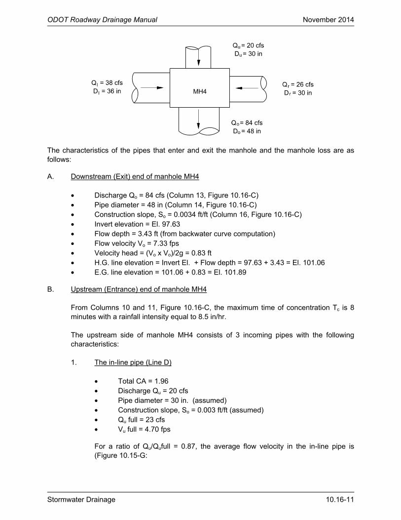
ODOT Roadway Drainage Manual November 2014
Stormwater Drainage 10.16-11
The characteristics of the pipes that enter and exit the manhole and the manhole loss are as follows:
A. Downstream (Exit) end of manhole MH4
• Discharge Qo = 84 cfs (Column 13, Figure 10.16-C) • Pipe diameter = 48 in (Column 14, Figure 10.16-C) • Construction slope, So = 0.0034 ft/ft (Column 16, Figure 10.16-C) • Invert elevation = El. 97.63 • Flow depth = 3.43 ft (from backwater curve computation) • Flow velocity Vo = 7.33 fps • Velocity head = (Vo x Vo)/2g = 0.83 ft • H.G. line elevation = Invert El. + Flow depth = 97.63 + 3.43 = El. 101.06 • E.G. line elevation = 101.06 + 0.83 = El. 101.89
B. Upstream (Entrance) end of manhole MH4
From Columns 10 and 11, Figure 10.16-C, the maximum time of concentration Tc is 8 minutes with a rainfall intensity equal to 8.5 in/hr. The upstream side of manhole MH4 consists of 3 incoming pipes with the following characteristics: 1. The in-line pipe (Line D)
• Total CA = 1.96 • Discharge Qu = 20 cfs • Pipe diameter = 30 in. (assumed) • Construction slope, So = 0.003 ft/ft (assumed) • Qu full = 23 cfs • Vu full = 4.70 fps
For a ratio of Qu/Qufull = 0.87, the average flow velocity in the in-line pipe is (Figure 10.15-G:
ODOT Roadway Drainage Manual November 2014
10.16-12 Stormwater Drainage
• Vu/Vu Full = 1.13 • Vu = 5.3 fps • Velocity head = (Vu x Vu)/2g = 0.44 ft
2. The right lateral pipe (Line B)
• Total CA = 2.544 • Discharge Qr = 26 cfs • Pipe diameter = 30 in. (assumed) • Construction slope, So = 0.008 ft/ft (assumed) • Qr full = 28 cfs • Vr full = 5.80 fps
For a ratio of Qu/Qu full = 0.93, the average flow velocity in the in-line pipe is (Figure 10.16-G): • Vu/Vu Full = 1.14 • Vr = 6.61 fps • Velocity head = (Vr x Vr)/2g = 0.68 ft
From Figure 10.16-D, the bend coefficient Kr = 0.7 for open channel flow. 3. The left lateral pipe (Line A)
• Total CA = 3.696 (Column 7, Figure 10.16-C) • Discharge Q1 = 38 cfs • Pipe diameter = 36 in. (Column 14, Figure 10.16-C) • Construction slope, So = 0.0034 ft/ft (Column 16, Figure 10.16-C) • Invert elevation = El. 98.63 • Q1 full = 39 cfs • V1 full = 5.50 fps
For a ratio of Q1/Q1 full = 0.97, the average flow velocity in the in-line pipe is (Figure 10.16-G): • V1/V1 Full = 1.15 • V1 = 6.3 fps • Velocity head = (Vr × Vr)/2g = 0.62 ft
From Figure 10.16-D, the bend coefficient K1 = 0.7 for open channel flow.

OD
OT
Road
way D
rainage Manual
N
ovem
ber 2014
Storm
water D
rainage 10.16-13
Fig
ure 10.16-G
— R
EL
AT
IVE
V, A
, Q IN
A C
IRC
UL
AR
PIP
E F
OR
AN
Y D
EP
TH
OF
FL
OW
, W
ITH
CO
NS
TA
NT
“N”
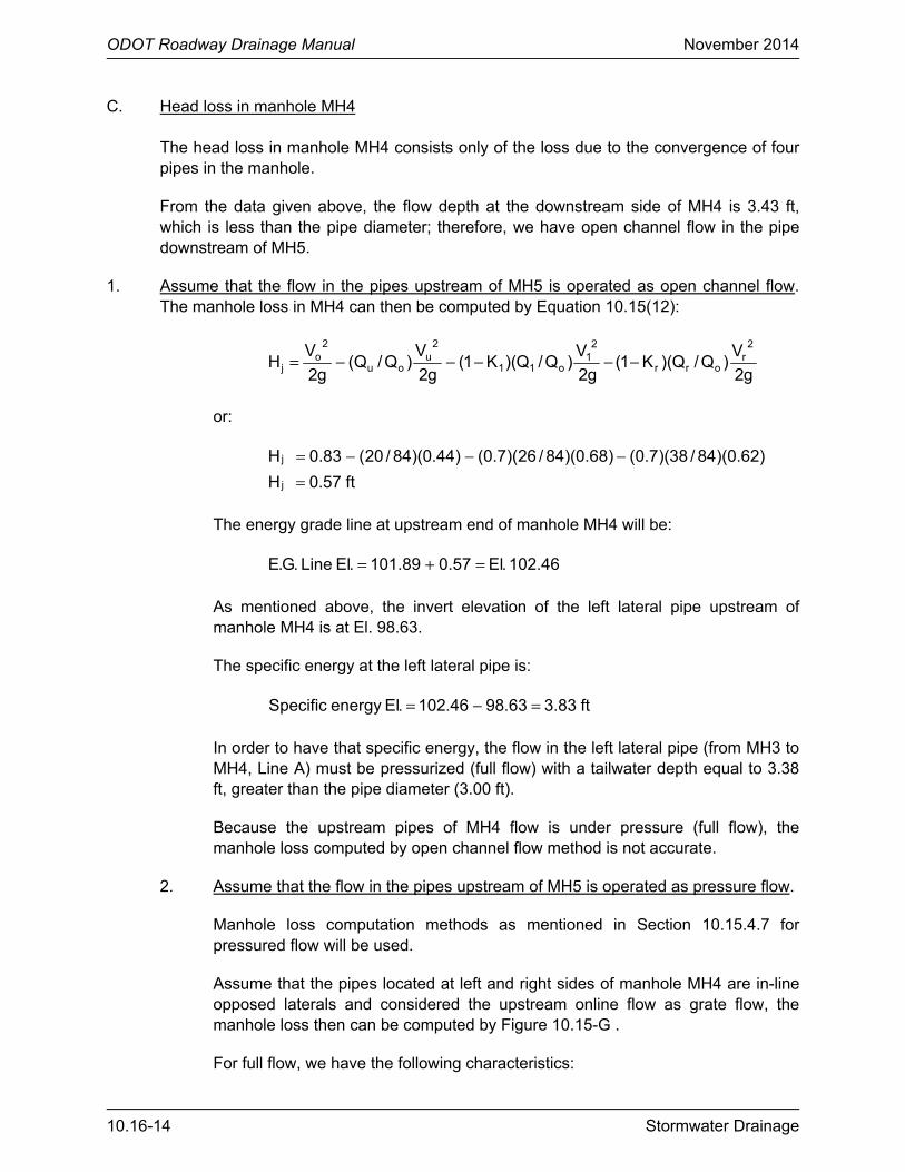
ODOT Roadway Drainage Manual November 2014
10.16-14 Stormwater Drainage
C. Head loss in manhole MH4 The head loss in manhole MH4 consists only of the loss due to the convergence of four pipes in the manhole.
From the data given above, the flow depth at the downstream side of MH4 is 3.43 ft, which is less than the pipe diameter; therefore, we have open channel flow in the pipe downstream of MH5.
1. Assume that the flow in the pipes upstream of MH5 is operated as open channel flow. The manhole loss in MH4 can then be computed by Equation 10.15(12):
g2
V)Q/Q)(K1(
g2
V)Q/Q)(K1(
g2
V)Q/Q(
g2
VH
2r
orr
21
o11
2u
ou
2o
j −−−−−=
or:
)62.0)(84/38)(7.0()68.0)(84/26)(7.0()44.0)(84/20(83.0Hj −−−=
ft57.0Hj =
The energy grade line at upstream end of manhole MH4 will be:
46.102.El57.089.101.ElLine.G.E =+=
As mentioned above, the invert elevation of the left lateral pipe upstream of manhole MH4 is at El. 98.63.
The specific energy at the left lateral pipe is:
ft83.363.9846.102.ElenergySpecific =−=
In order to have that specific energy, the flow in the left lateral pipe (from MH3 to MH4, Line A) must be pressurized (full flow) with a tailwater depth equal to 3.38 ft, greater than the pipe diameter (3.00 ft).
Because the upstream pipes of MH4 flow is under pressure (full flow), the manhole loss computed by open channel flow method is not accurate.
2. Assume that the flow in the pipes upstream of MH5 is operated as pressure flow.
Manhole loss computation methods as mentioned in Section 10.15.4.7 for pressured flow will be used.
Assume that the pipes located at left and right sides of manhole MH4 are in-line opposed laterals and considered the upstream online flow as grate flow, the manhole loss then can be computed by Figure 10.15-G .
For full flow, we have the following characteristics:
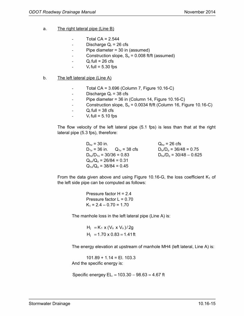
ODOT Roadway Drainage Manual November 2014
Stormwater Drainage 10.16-15
a. The right lateral pipe (Line B)
- Total CA = 2.544 - Discharge Qr = 26 cfs - Pipe diameter = 30 in (assumed) - Construction slope, So = 0.008 ft/ft (assumed) - Qr full = 26 cfs - Vr full = 5.30 fps
b. The left lateral pipe (Line A)
- Total CA = 3.696 (Column 7, Figure 10.16-C) - Discharge Qr = 38 cfs - Pipe diameter = 36 in (Column 14, Figure 10.16-C) - Construction slope, So = 0.0034 ft/ft (Column 16, Figure 10.16-C) - Qr full = 38 cfs - Vr full = 5.10 fps
The flow velocity of the left lateral pipe (5.1 fps) is less than that at the right lateral pipe (5.3 fps), therefore:
Dhv = 30 in. Qhv = 26 cfs D1v = 36 in. Q1v = 38 cfs Dlv/Do = 36/48 = 0.75 Dhv/D1v = 30/36 = 0.83 Dhv/Do = 30/48 – 0.625 Qhv/Qo = 26/84 = 0.31 Q1v/Qo = 38/84 = 0.45
From the data given above and using Figure 10.16-G, the loss coefficient K1 of the left side pipe can be computed as follows:
Pressure factor H = 2.4 Pressure factor L = 0.70 K1 = 2.4 – 0.70 = 1.70
The manhole loss in the left lateral pipe (Line A) is:
g2/)VxV(xKH oo1j =
ft41.183.0x70.1Hj ==
The energy elevation at upstream of manhole MH4 (left lateral, Line A) is: 101.89 + 1.14 = El. 103.3 And the specific energy is:
ft67.463.9830.103.ELenergeySpecific =−=

ODOT Roadway Drainage Manual November 2014
10.16-16 Stormwater Drainage
In order to have that specific energy, the flow in the left lateral pipe (from MH3 to MH4, Line A) must be pressurized (full flow) with a tailwater depth equal to 4.22 ft, greater than the pipe diameter (3.00 ft), therefore, the assumption of full flow is correct.
From Figure 10.15-C, at design discharge Q = 39 cfs, the flow velocity is 5.5 fps and the velocity head is 0.47 ft in the left lateral pipe, upstream of manhole MH4. The hydraulic grade line elevation at upstream side of MH4 (left lateral, Line A) will be:
ft83.102.El47.030.103.Elline.G.H =−=
D. H.G. Line Elevation Check
From Figure 10.16-B, the elevation of the top of manhole MH4 is at El. 105.0 or about 2.17 ft higher than the H.G. line elevation. This distance is greater than the 1 ft clearance as required by design criteria, therefore, the design is acceptable.
10.16.6 Manhole MH3
Manhole MH3 is located 300 ft upstream of manhole MH4 and is a reinforced concrete rectangular manhole as shown below:
The characteristics of the pipes that enter and exit the manhole and the manhole loss are as follows:
A. Downstream (exit) End of Manhole MH3
• Discharge Qo = 39 cfs (Column 13, Figure 10.16-C)
• Pipe diameter = 36 in (Column 14, Figure 10.16-C)
• Construction slope, So = 0.0034 ft/ft (Column 16, Figure 10.16-C)
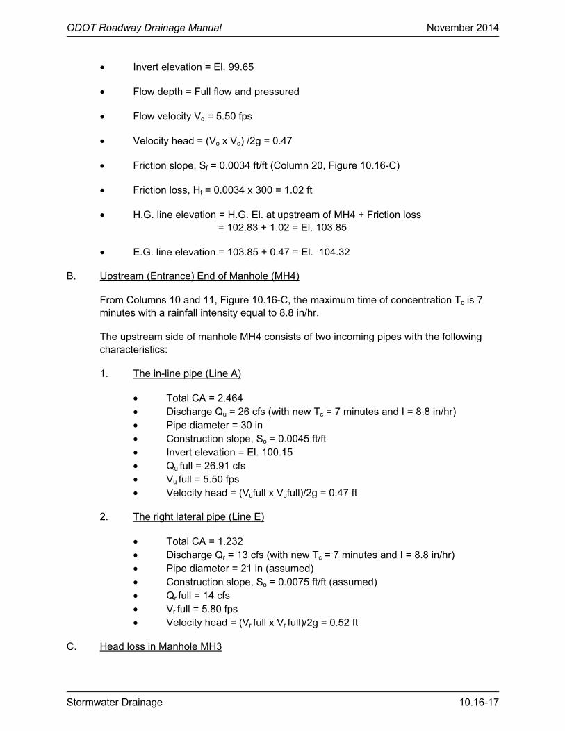
ODOT Roadway Drainage Manual November 2014
Stormwater Drainage 10.16-17
• Invert elevation = El. 99.65
• Flow depth = Full flow and pressured
• Flow velocity Vo = 5.50 fps
• Velocity head = (Vo x Vo) /2g = 0.47
• Friction slope, Sf = 0.0034 ft/ft (Column 20, Figure 10.16-C)
• Friction loss, Hf = 0.0034 x 300 = 1.02 ft
• H.G. line elevation = H.G. El. at upstream of MH4 + Friction loss = 102.83 + 1.02 = El. 103.85
• E.G. line elevation = 103.85 + 0.47 = El. 104.32
B. Upstream (Entrance) End of Manhole (MH4)
From Columns 10 and 11, Figure 10.16-C, the maximum time of concentration Tc is 7 minutes with a rainfall intensity equal to 8.8 in/hr.
The upstream side of manhole MH4 consists of two incoming pipes with the following characteristics:
1. The in-line pipe (Line A)
• Total CA = 2.464 • Discharge Qu = 26 cfs (with new Tc = 7 minutes and I = 8.8 in/hr) • Pipe diameter = 30 in • Construction slope, So = 0.0045 ft/ft • Invert elevation = El. 100.15 • Qu full = 26.91 cfs • Vu full = 5.50 fps • Velocity head = (Vufull x Vufull)/2g = 0.47 ft
2. The right lateral pipe (Line E)
• Total CA = 1.232 • Discharge Qr = 13 cfs (with new Tc = 7 minutes and I = 8.8 in/hr) • Pipe diameter = 21 in (assumed) • Construction slope, So = 0.0075 ft/ft (assumed) • Qr full = 14 cfs • Vr full = 5.80 fps • Velocity head = (Vr full x Vr full)/2g = 0.52 ft
C. Head loss in Manhole MH3

ODOT Roadway Drainage Manual November 2014
10.16-18 Stormwater Drainage
The head loss in manhole MH3 consists of the loss due to the convergence of three pipes in the manhole. From the data given above, the outflow at downstream side of MH3 is flowing full and pressured. Assume that the flow in the pipes that enter MH3 is also pressured. The manhole loss in MH3 then can be computed by the pressured flow design method in Section 10.15.5.
Because there is no grate flow involved and because the ratio of D1/Do = 21/36 = 0.58 < 0.60, Figure 10.15-K will be used.
For Du/Do = 30/36 = 0.833 and Qu/Qo = 26/39 = 0.67, the loss coefficient Ku = K1 = 0.70 and the loss in manhole MH3 is:
ft33.047.0x70.02VkH
g
2o
bj ===
The energy elevation at upstream (Line A) of manhole MH3 is:
65.104.El33.032.104.Elline.G.E =+=
The specific energy at the in-line pipe is:
ft50.415.10065.104.ElenergySpecific =−=
In order to have that specific energy, the flow in the in-line pipe (from MH2 to MH3, Line A) must be pressurized (full flow) with a tailwater depth equal to 4.03 ft, greater than the pipe diameter (2.50 ft).
The velocity head for full flow in the in-line pipe is 0.47 ft as mentioned above. Therefore, the H.G. line elevation in the in-line, upstream side of MH3 is:
18.104.El47.065.104.Elline.G.H =−=
D. H.G. Line Elevation Check
From Figure 10.16-B, the elevation of the top of manhole MH3 is at El. 106.0 or about 1.82 ft higher than the H.G. line elevation.
This distance is greater than the 1 ft clearance as required by design criteria; therefore, the design is acceptable.
10.16.7 Manhole MH2
Manhole MH2 is located at 300 ft upstream of manhole MH3 and is a reinforced concrete rectangular manhole as shown below:
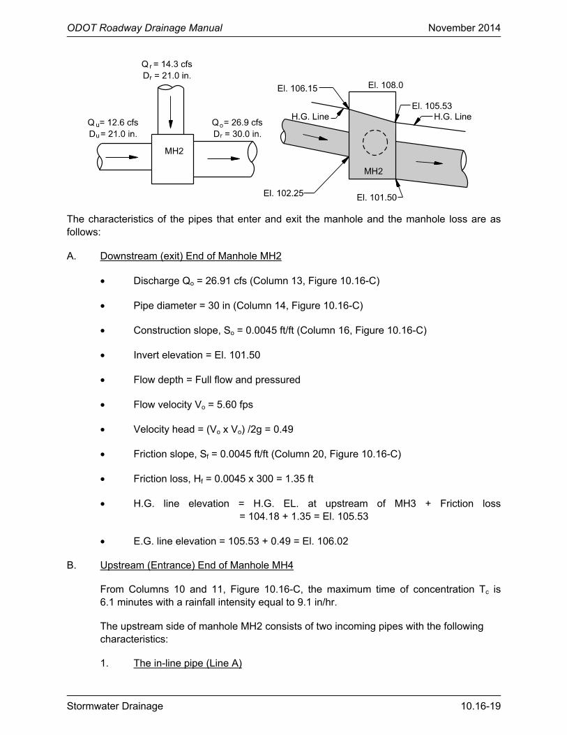
ODOT Roadway Drainage Manual November 2014
Stormwater Drainage 10.16-19
The characteristics of the pipes that enter and exit the manhole and the manhole loss are as follows:
A. Downstream (exit) End of Manhole MH2
• Discharge Qo = 26.91 cfs (Column 13, Figure 10.16-C)
• Pipe diameter = 30 in (Column 14, Figure 10.16-C)
• Construction slope, So = 0.0045 ft/ft (Column 16, Figure 10.16-C)
• Invert elevation = El. 101.50
• Flow depth = Full flow and pressured
• Flow velocity Vo = 5.60 fps
• Velocity head = (Vo x Vo) /2g = 0.49
• Friction slope, Sf = 0.0045 ft/ft (Column 20, Figure 10.16-C)
• Friction loss, Hf = 0.0045 x 300 = 1.35 ft
• H.G. line elevation = H.G. EL. at upstream of MH3 + Friction loss = 104.18 + 1.35 = El. 105.53
• E.G. line elevation = 105.53 + 0.49 = El. 106.02
B. Upstream (Entrance) End of Manhole MH4
From Columns 10 and 11, Figure 10.16-C, the maximum time of concentration Tc is 6.1 minutes with a rainfall intensity equal to 9.1 in/hr.
The upstream side of manhole MH2 consists of two incoming pipes with the following characteristics:
1. The in-line pipe (Line A)

ODOT Roadway Drainage Manual November 2014
10.16-20 Stormwater Drainage
• Total CA = 1.152 • Discharge Qu = 12.6 cfs • Pipe diameter = 21 in • Construction slope, So = 0.0065 ft/ft • Qufull = 13.00 cfs • Vufull = 5.30 fps • Velocity head = (Vufull x Vufull)/2g = 0.44 ft
2. The right lateral pipe (Line F)
• Total CA = 1.312 • Discharge Qr = 14.3 cfs • Pipe diameter = 21 in (assumed) • Construction slope, So = 0.0080 ft/ft (assumed) • Qrfull = 14 cfs • Vrfull = 6.10 fps • Velocity head = (Vrfull × Vrfull)/2g = 0.58 ft
C. Head loss in manhole MH2
The head loss in manhole MH2 consists of only the loss due to the convergence of three pipes in the manhole. From the data given above, the outflow at downstream side of MH2 is flowing full and pressured.
Assume that the flow in the pipes that enter MH2 is pressured. The manhole loss in MH2 then can be computed by pressured flow design method.
Because there is no grate flow involved and because the ratio of Dr/Do = 21/30 = 0.70 > 0.60, Figure 10.15-J will be used to find the in-line loss coefficient Ku.
Assume that the width B of the manhole MH2 is equal to 42 in, so the ratio B/Do = 42/30 = 1.4.
For Du/Do = 0.70 and B/Do = 1.4, read the value Ku = 2.1 from the lower part of Figure 10.15-J.
For (Qu/Qo)(Do/Du) = (12.6/26.91) (30/21) = 0.67, the value of Mu = 0.55 from the upper part of Figure 10.15-J.
So:
16.11.2x55.0KtcoefficienLoss u ==
And the loss in manhole MH2 is:
ft57.049.0x16.12VKH
g
2o
uj ===
The energy elevation at upstream (Line A) of manhole MH2 is:

ODOT Roadway Drainage Manual November 2014
Stormwater Drainage 10.16-21
59.106.El57.002.106.Elline.G.E =+=
The specific energy at the in-line pipe, upstream of MH2 is:
ft34.425.10259.106.ElenergySpecific =−=
In order to have that specific energy, the flow in the upstream pipe (from MH1 to MH2, Line A) must be pressurized (full flow) with a tailwater depth equal to 4.03 ft, greater than the pipe diameter (2.50 ft).
The velocity head for in the in-line upstream pipe is 0.44 ft for full flow as mentioned above. Therefore, the H.G. line elevation in the in-line, upstream side of MH2 is:
15.106.El44.059.106.Elline.G.H =−=
D. H.G. Line Elevation Check
From Figure 10.16-B, the elevation of the top of manhole MH2 is at El. 108.0 or about 1.85 ft higher than the H.G. line elevation.
This distance is greater than the 1 ft clearance as required by design criteria, therefore, the design is acceptable.
10.16.8 Manhole MH1
Manhole MH1 is located 300 ft upstream of manhole MH2 and is a reinforced concrete rectangular manhole as shown below:
The characteristics of the pipes that enter and exit the manhole and the manhole loss are as follows:
A. Downstream (exit) End of Manhole MH1
• Discharge Qo = 13.00 cfs (Column 13, Figure 10.16-C)
ODOT Roadway Drainage Manual November 2014
10.16-22 Stormwater Drainage
• Pipe diameter = 21 in (Column 14, Figure 10.16-C)
• Construction slope, So = 0.0065 ft/ft (Column 16, Figure 10.16-C)
• Invert elevation = El. 104.20
• Flow depth = Full flow and pressured
• Flow velocity Vo = 5.30 fps
• Velocity head = (Vo x Vo) /2g = 0.44
• Friction slope, Sf = 0.0065 ft/ft (Column 20, Figure 10.16-C)
• Friction loss, Hf = 0.0065 x 300 = 1.95 ft
• H.G. line elevation = H.G. El. at upstream of MH4 + Friction loss = 106.15 + 1.95 = El. 108.10
• E.G. line elevation = 108.10 + 0.44 = El. 108.54
B. Upstream (Entrance) End of Manhole (MH1)
From Columns 10 and 11, Figure 10.16-C, the maximum time of concentration Tc is 5.2 minutes with a rainfall intensity equal to 9.4 in/hrs.
The upstream side of manhole MH1 consists of a 21-in pipe, 90-degree bend with the following characteristics:
• Total CA = 1.152 • Discharge Qu = 13.0 cfs • Pipe diameter = 21 in • Construction slope, So = 0.0065 ft/ft • Qufull = 13.00 cfs • Vufull = 5.30 fps • Velocity head = (Vufull × Vufull)/2g = 0.44 ft
C. Head loss in manhole MH1
The head loss in manhole MH1 consists only of the loss due to 90° bend. Assume that deflector will be used in the manhole. The manhole loss in MH1 can be computed by pressure flow design methods.
From Figure 10.15-E, the loss coefficient K for a 90° bend with deflector in pressured flow is K = 1.00.
And the loss in manhole MH1 is:
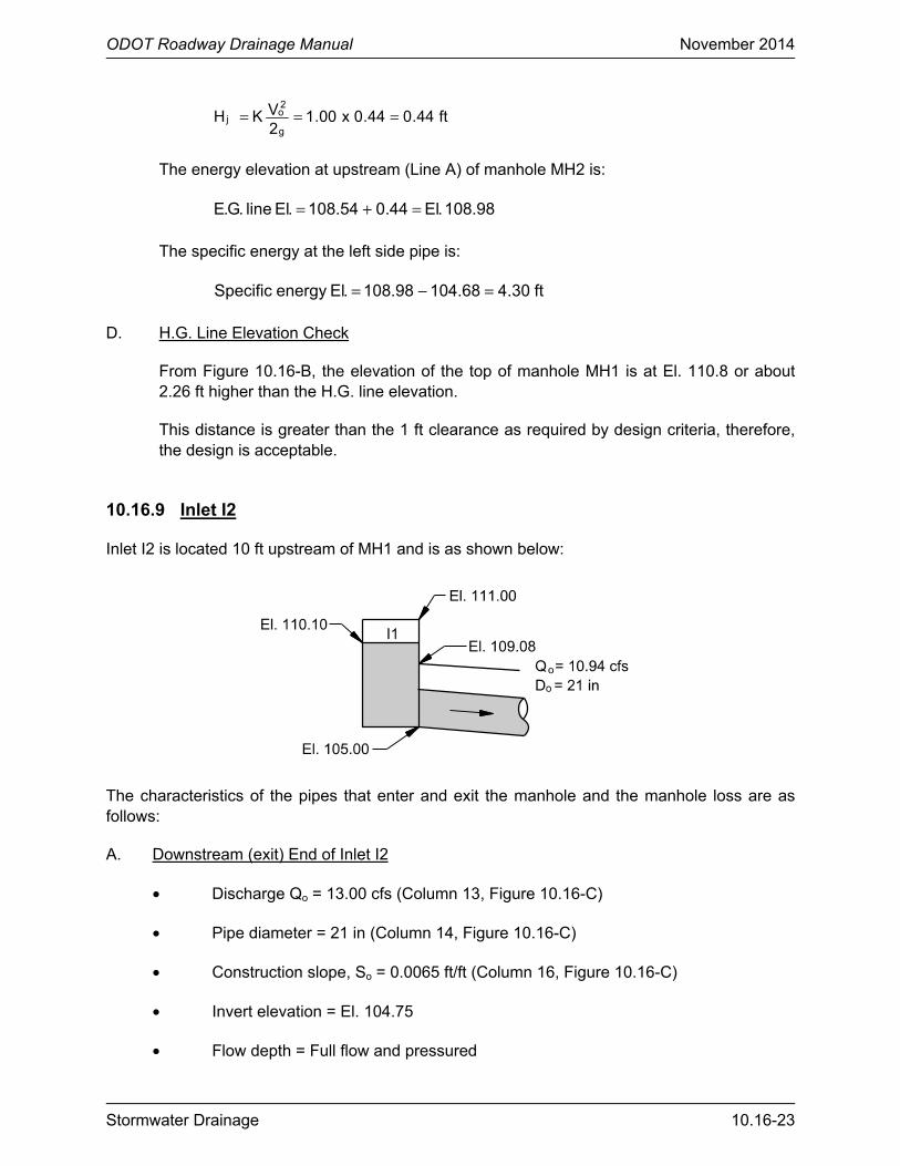
ODOT Roadway Drainage Manual November 2014
Stormwater Drainage 10.16-23
ft44.044.0x00.12VKH
g
2o
j ===
The energy elevation at upstream (Line A) of manhole MH2 is:
98.108.El44.054.108.Elline.G.E =+=
The specific energy at the left side pipe is:
ft30.468.10498.108.ElenergySpecific =−=
D. H.G. Line Elevation Check
From Figure 10.16-B, the elevation of the top of manhole MH1 is at El. 110.8 or about 2.26 ft higher than the H.G. line elevation.
This distance is greater than the 1 ft clearance as required by design criteria, therefore, the design is acceptable.
10.16.9 Inlet I2
Inlet I2 is located 10 ft upstream of MH1 and is as shown below:
The characteristics of the pipes that enter and exit the manhole and the manhole loss are as follows:
A. Downstream (exit) End of Inlet I2
• Discharge Qo = 13.00 cfs (Column 13, Figure 10.16-C)
• Pipe diameter = 21 in (Column 14, Figure 10.16-C)
• Construction slope, So = 0.0065 ft/ft (Column 16, Figure 10.16-C)
• Invert elevation = El. 104.75
• Flow depth = Full flow and pressured
ODOT Roadway Drainage Manual November 2014
10.16-24 Stormwater Drainage
• Flow velocity Vo = 5.30 fps
• Velocity head = (Vo x Vo) /2g = 0.44
• Friction slope, Sf = 0.0065 ft/ft (Column 20, Figure 10.16-C)
• Friction loss, Hf = 0.0065 x 10 = 0.07 ft
• H.G. line elevation = H.G. El. at upstream of MH4 + Friction loss = 108.54 + 0.07 = El. 108.61
• E.G. line elevation = 108.61 + 0.44 = El. 109.05
B. Upstream (Entrance) End of Inlet I2
From Columns 10 and 11, Figure 10.16-C, the maximum time of concentration Tc is 5.2 minutes with a rainfall intensity equal to 9.4 in/hrs.
The upstream side of manhole MH1 consists of a 21-in pipe with the following characteristics:
• Total CA = 0.96 • Discharge Qu = 10.8 cfs • Pipe diameter = 21 in • Construction slope, So = 0.0050 ft/ft • Qu full = 11.00 cfs • Vu full = 4.50 fps • Velocity head = (Vu full × Vu full)/2g = 0.32 ft
The flow through inlet I2 is:
• Total CA = 0.192 • Discharge Qg = 2.2 cfs
C. Head loss in Inlet I2
The head loss in inlet I2 is negligible because the pipes at upstream and downstream side are of the same diameter and there is no deflection of the pipe line.
The energy elevation at upstream (Line A) of inlet I2 is at the same elevation as downstream or El. 109.05.
The hydraulic grade line elevation at upstream side of I2 is:
83.108.El32.005.109.Elline.G.H =−=
D. H.G. Line Elevation Check
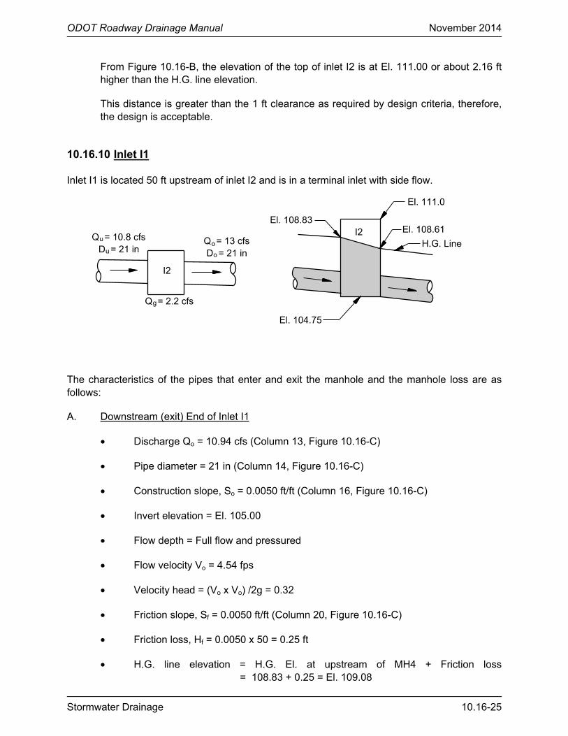
ODOT Roadway Drainage Manual November 2014
Stormwater Drainage 10.16-25
From Figure 10.16-B, the elevation of the top of inlet I2 is at El. 111.00 or about 2.16 ft higher than the H.G. line elevation.
This distance is greater than the 1 ft clearance as required by design criteria, therefore, the design is acceptable.
10.16.10 Inlet I1
Inlet I1 is located 50 ft upstream of inlet I2 and is in a terminal inlet with side flow.
The characteristics of the pipes that enter and exit the manhole and the manhole loss are as follows:
A. Downstream (exit) End of Inlet I1
• Discharge Qo = 10.94 cfs (Column 13, Figure 10.16-C)
• Pipe diameter = 21 in (Column 14, Figure 10.16-C)
• Construction slope, So = 0.0050 ft/ft (Column 16, Figure 10.16-C)
• Invert elevation = El. 105.00
• Flow depth = Full flow and pressured
• Flow velocity Vo = 4.54 fps
• Velocity head = (Vo x Vo) /2g = 0.32
• Friction slope, Sf = 0.0050 ft/ft (Column 20, Figure 10.16-C)
• Friction loss, Hf = 0.0050 x 50 = 0.25 ft
• H.G. line elevation = H.G. El. at upstream of MH4 + Friction loss = 108.83 + 0.25 = El. 109.08

ODOT Roadway Drainage Manual November 2014
10.16-26 Stormwater Drainage
• E.G. line elevation = 109.08 + 0.32 = El. 109.40
B. Head Loss in Inlet I1
The head loss in inlet I1 can be computed by using Figure 10.15-L. By following the detailed instruction on how to use this chart, the hydraulics designer will find that the terminal inlet loss coefficient K is equal to 3.2 and the head loss in inlet I1 is:
ft02.132.0x2.3Ht ==
The hydraulic grade line elevation at inlet I1 then becomes:
The hydraulic grade line elevation at inlet of I1 is:
10.110.El02.108.109.Elline.G.H =+=
C. C.G. Line Elevation Check
From Figure 10.16-B, the elevation of the top of inlet I1 is at El. 111.00 or about 0.90 ft higher than the H.G. line elevation.
This distance is greater than the 1 ft clearance as required by design criteria, therefore, the design is acceptable.
The design of Line A is acceptable and Figure 10.16-C can be considered as the final design.

ODOT Roadway Drainage Manual November 2014
Stormwater Drainage 10.17-1
10.17 REFERENCES
1. AASHTO. Drainage Manual. Washington, DC : Techncial Committee on Hydrology and Hydraulics, American Association of State Highway and Transportation Officials, 2012.
2. FHWA. Urban Drainage Design Manual, Hydraulic Engineering Circular No. 22, 3rd Edition. Washington, DC : Federal Highway Administration, 2009. FHWA-NHI-10-009.
3. AASHTO. Highway Drainage Guidelines, 4th Edition. Washington, DC : Technical Committee on Hydrology and Hydraulics, American Association of State Highway and Transportation Officials, 2007.
4. NCHRP. Improved Surface Drainage of Pavements: Final Report. Washington, DC : National Cooperative Highway Research Program, Transportation Research Board, 1998. Web Doc 16.
5. —. Proposed Design Guidelines for Reducing Hydroplaning on New and Rehabilitated Pavements. Washington, DC : National Cooperative Highway Research Program, Transportation Research Board, 1999. Results Digest, Issue Number 243.
6. USBR. Design of Small Canal Structures. Denver, CO : U.S. Bureau of Reclamation, 1978.
7. AASHTO. A Policy on Geometric Design of Highways and Streets, 6th Edition. Washington, DC : Technical Committee on Geometric Design, American Association of State Highway and Transportation Officials, 2011.
8. FHWA. Design Charts for Open Channel Flow, Hydraulic Design Series No. 3. Washington, DC : Federal Highway Administration, 1961. FHWA-EPD-86-102.
9. Sangster, W.M. Pressure Changes at Storm Drain Junctions. Columbia, MO : University of Missouri, 1958. Engineering Series Bulletin No. 41.

ODOT Roadway Drainage Manual November 2014
10.17-2 Stormwater Drainage