Chapter 10 DOMAIN THEORY AND FIXED-POINT...

341

Chapter 10DOMAIN THEORY ANDFIXED-POINT SEMANTICS

Although we did not stress the point in Chapter 9, the notation ofdenotational semantics is built upon that of the lambda calculus. Thepurpose of denotational semantics is to provide mathematical descrip-

tions of programming languages independent of their operational behavior.The extended lambda calculus serves as a mathematical formalism, ametalanguage, for denotational definitions. As with all mathematical formal-isms, we need to know that the lambda calculus has a model to ensure thatthe definitions are not meaningless.

Furthermore, denotational definitions, as well as programming languages ingeneral, rely heavily on recursion, a mechanism whose description we de-ferred in the discussion of the lambda calculus in Chapter 5. Normally a userof a programming language does not care about the logical foundations ofdeclarations, but we maintain that serious questions can be raised concern-ing the validity of recursion. In this chapter we justify recursive definitions toguarantee that they actually define meaningful objects.

10.1 CONCEPTS AND EXAMPLES

Programmers use recursion to define functions and procedures as subpro-grams that call themselves and also to define recursive data structures. Mostimperative programming languages require the use of pointers to declarerecursive data types such as (linked) lists and trees. In contrast, many func-tional programming languages allow the direct declaration of recursive types.Rather than investigating recursive types in an actual programming language,we study recursive data declarations in a wider context. In this introductorysection we consider the problems inherent in recursively defined functionsand data and the related issue of nontermination.

342 CHAPTER 10 DOMAIN THEORY AND FIXED-POINT SEMANTICS

Recursive Definitions of Functions

When we define a symbol in a denotational definition or in a program, weexpect that the symbol can be replaced by its meaning wherever it occurs. Inparticular, we expect that the symbol is defined in terms of other (preferablysimpler) concepts so that any expression involving the symbol can be ex-pressed by substituting its definition. With this concept in mind, considertwo simple recursive definitions:

f(n) = if n=0 then 1 else f(n–1)

g(n) = if n=0 then 1 else g(n+1).

The purpose of these definitions is to give meaning to the symbols “f” and “g”.Both definitions can be expressed in the applied lambda calculus as

define f = λn . (if (zerop n) 1 (f (sub n 1)))

define g = λn . (if (zerop n) 1 (g (succ n))).

Either way, these definitions fail the condition that the defined symbol canbe replaced by its meaning, since that meaning also contains the symbol.The definitions are circular. The best we can say is that recursive “defini-tions” are equations in the newly defined symbol. The meaning of the symbolwill be a solution to the equation, if a solution exists. If the equation hasmore than one solution, we need some reason for choosing one of those solu-tions as the meaning of the new symbol.

An analogous situation can be seen with a mathematical equation that re-sembles the recursive definitions:

x = x2 – 4x + 6.

This “definition” of x has two solutions, x=2 and x=3. Other similar defini-tions of x, such as x = x+5, have no solutions at all, while x = x2/x hasinfinitely many solutions. We need to describe conditions on a recursive defi-nition of a function, really a recursion equation, to guarantee that at leastone solution exists and a reason for choosing one particular solution as themeaning of the function.

For the examples considered earlier, we will describe in this chapter a meth-odology that enables us to show that the equation in f has only one solution(λn . 1), but the equation in g has many solutions, including

(λn . 1) and (λn . if n=0 then 1 else undefined).

One purpose of this chapter is to develop a “fixed-point” semantics that givesa consistent meaning to recursive definitions of functions.

34310.1 CONCEPTS AND EXAMPLES

Recursive Definitions of Sets (Types)

Recursively defined sets occur in both programming languages and specifi-cations of languages. Consider the following examples:

1. The BNF specification of Wren uses direct recursion in specifying the syn-tactic category of identifiers,

<identifier> ::= <letter> | <identifier> <letter> | <identifier> <digit>,

and indirect recursion in many places, such as,

<command> ::= if <boolean expr> then <command seq> end if

<command seq> ::= <command> | <command> ; <command seq>.

2. The domain of lists of natural numbers N may be provided in a functionalprogramming language according to the definition:

List = {nil } ∪ (N x List) where nil represents the empty list.

Scheme lists have essentially this form using “cons” as the constructoroperation forming ordered pairs in N x List. Standard ML allows data typedeclarations following this pattern.

3. A model for the (pure) lambda calculus requires a domain of values thatare manipulated by the rules of the system. These values incorporatevariables as primitive objects and functions that may act on any values inthe domain, including any of the functions. If V denotes the set of vari-ables and D→D represents the set of functions from set D to D, the do-main of values for the lambda calculus can be “defined” by D = V ∪ (D→D).

The third example presents major problems if we analyze the cardinality ofthe sets involved. We give the critical results without going into the details ofmeasuring the cardinality of sets. It suffices to mention that the sizes of setsare compared by putting their elements into a one-to-one correspondence.We denote the cardinality of a set A by |A| with the following properties:

1. |A| ≤ |B| if there is a one-to-one function A→B.

2. |A| = |B| if there is a one-to-one and onto function A→B (which can beshown to be equivalent to |A| ≤ |B| and |B| ≤ |A|).

3. |A| < |B| if |A| ≤ |B| but not |A| ≥ |B|.

Two results about cardinalities of sets establish the problem with the recur-sive “definition” of D:

1. In the first use of “diagonalization” as a proof method, Georg Cantorproved that for any set A, |A| < |P(A)| where P(A) is the power setof A—that is, the set of all subsets of A.


2. If |A| > 1, then |P(A)| ≤ |A→A|.

Since D→D is a subset of D by the definition, |D→D| ≤ |D|. Therefore,|D→D| ≤ |D| < |P(D)| ≤ |D→D|,

which is clearly a contradiction.

One way to provide a solution to the recursion equation D = V ∪ (D→D) is torestrict the membership in the set of functions D→D by putting a “structure”on the sets under consideration and by requiring that functions are well-behaved relative to the structure. Although the solution to this recursionequation is beyond the scope of this book (see the further readings at the endof this chapter), we study this structure carefully for the intuition that itprovides about recursively defined functions and sets.

Modeling Nontermination

Any programming language that provides (indefinite) iteration or recursivelydefined functions unfortunately also allows a programmer to write nontermi-nating programs. Specifying the semantics of such a language requires amechanism for representing nontermination. At this point we preview do-main theory by considering how it handles nontermination. Domain theoryis based on a relation of definedness. We say x ⊆ y if x is less defined than orequal to y. This means that the information content of x is contained in theinformation content of y. Each domain (structured set) contains a least ele-ment ⊥, called bottom, representing the absence of information. Bottom canbe viewed as the result of a computation that fails to terminate normally. Byadding a bottom element to every domain, values that produce no outcomeunder a function can be represented by taking ⊥ as the result. This simpleidea enables us to avoid partial functions in describing the semantics of aprogramming language, since values for which a function is undefined mapto the bottom element in the codomain.

Dana Scott developed domain theory to provide a model for the lambda cal-culus and thereby provide a consistent foundation for denotational seman-tics. Without such a foundation, we have no reason to believe that denotationaldefinitions really have mathematical meaning. At the same time, domaintheory gives us a valid interpretation for recursively defined functions andtypes.

In this chapter we first describe the structure supplied to sets by domaintheory, and then we investigate the semantics of recursively defined func-tions via fixed-point theory. Finally, we use fixed points to give meaning torecursively defined functions in the lambda calculus, implementing them byextending the lambda calculus evaluator described in Chapter 5.

345

Exercises

1. Write a recursive definition of the factorial function in the lambda calcu-lus using define.

2. Give a recursive definition of binary trees whose leaf nodes contain naturalnumber values.

3. Suppose A is a finite set with |A| = n. Show that |P(A)| = 2n and |A→A|= nn.

4. Let A be an arbitrary set. Show that it is impossible for f : A→P(A) to be aone-to-one and onto function. Hint: Consider the set X = {a∈A | a∉f(a)}.

5. Prove that |P(A)| ≤ |A→A| for any set A with |A| ≥ 2. Hint: Consider thecharacteristic functions of the sets in P(A).

10.2 DOMAIN THEORY

The structured sets that serve as semantic domains in denotational seman-tics are similar to the structured sets called lattices, but these domains haveseveral distinctive properties. Domains possess a special element ⊥, calledbottom , that denotes an undefined element or simply the absence of infor-mation. A computation that fails to complete normally produces ⊥ as itsresult. Later in this section we describe how the bottom element of a domaincan be used to represent the nontermination of programs, since a programthat never halts is certainly an undefined object. But first we need to definethe structural properties of the sets that serve as domains.

Definition : A partial or der on a set S is a relation ⊆ with the followingproperties:

1. ⊆ is reflexive : x ⊆ x for all x∈S.

2. ⊆ is transitive : (x ⊆ y and y ⊆ z) implies x ⊆ z for all x,y,z∈S.

3. ⊆ is antisymmetric : (x ⊆ y and y ⊆ x) implies x = y for all x,y∈S. ❚

Definition : Let A be a subset of S.

1. A lower bound of A is an element b∈S such that b ⊆ x for all x∈A.

2. An upper bound of A is an element u∈S such that x ⊆ u for all x∈A.

3. A least upper bound of A, written lub A, is an upper bound of A with theproperty that for any upper bound m of A, lub A ⊆ m. ❚

Example 1 : The subset relation ⊆ on the power set P({1,2,3}) is a partial orderas shown by the Hasse diagram in Figure 10.1. The main idea of a Hasse

10.2 DOMAIN THEORY


diagram is to represent links between distinct items where no other valuesintervene. The reflexive and transitive closure of this “minimal” relation formsthe ordering being defined. We know that the subset relation is reflexive,transitive, and antisymmetric. Any subset of P({1,2,3}) has lower, upper, andleast upper bounds. For example, if A = { {1}, {1,3}, {3} }, both {1,2,3} and {1,3}are upper bounds of A, ∅ is a lower bound of A, and lub A = {1,3}. ❚

{ 1,2,3 }

{ 1,2 } { 1,3 } { 2,3 }

{ 1 } { 2 } { 3 }

∅

Figure 10.1: Partial order on P({1,2,3})

In addition to possessing a partial ordering, the structured sets of domaintheory require a “smallest” element and the existence of limits for sequencesthat admit a certain conformity.

Definition : An ascending chain in a partially ordered set S is a sequence ofelements {x1, x2, x3, x4, …} with the property x1 ⊆ x2 ⊆ x3 ⊆ x4 ⊆ …. ❚

Remember that the symbol ⊆ stands for an arbitrary partial order, not neces-sarily the subset relation. Each item in an ascending chain must containinformation that is consistent with its predecessor in the chain; it may beequal to its predecessor or it may provide additional information.

Definition : A complete partial or der (cpo) on a set S is a partial order ⊆with the following properties:

1. There is an element ⊥∈S for which ⊥ ⊆ x for all x∈S.

2. Every ascending chain in S has a least upper bound in S. ❚

Sets with complete partial orders serve as the semantic domains indenotational semantics. On these domains, ⊆ is thought of as the relationapproximates or is less defined than or equal to . View x ⊆ y as asserting

347

that y has at least as much information content as x does, and that theinformation in y is consistent with that in x. In other words, y is a consistent(possibly trivial) extension of x in terms of information.

The least upper bound of an ascending chain summarizes the informationthat has been accumulated in a consistent manner as the chain progresses.Since an ascending chain may have an infinite number of distinct values, theleast upper bound acts as a limit value for the infinite sequence. On theother hand, a chain may have duplicate elements, since ⊆ includes equality,and a chain may take a constant value from some point onward. Then theleast upper bound is that constant value.

Example 1 (r evisited) : P({1,2,3}) with ⊆ is a complete partial order. If S isa set of subsets of {1,2,3}, lub S = ∪{X | X∈S}, and ∅ serves as bottom.Note that every ascending chain in P({1,2,3}) is a finite subset of P({1,2,3})—for example, the chain with x1={2}, x2={2,3}, x3={1,2,3}, and xi={1,2,3} forall i≥4. ❚

Example 2 : Define m ⊆ n on the set S = {1,2,3,5,6,15} as the divides relation,m|n (n is a multiple of m). The set S with the divides ordering is a completepartial order with 1 as the bottom element, and since each ascending chainis finite, its last element serves as the least upper bound. Figure 10.2 gives aHasse diagram for this ordered set. Observe that the elements of the set lieon three levels. Therefore no ascending chain can have more than threedistinct values. ❚

6 15

2 3 5

1

Figure 10.2: Partial order “divides” on {1,2,3,5,6,15}

These complete partially ordered sets have a lattice-like structure but neednot be lattices. Lattices possess the property that any two elements have aleast upper bound and a greatest lower bound. A complete lattice also satis-fies the condition that any subset has a least upper bound and a greatestlower bound. Observe that {1,2,3,5,6,15} with “divides” is not a lattice since{6,15} has no least upper bound.

10.2 DOMAIN THEORY


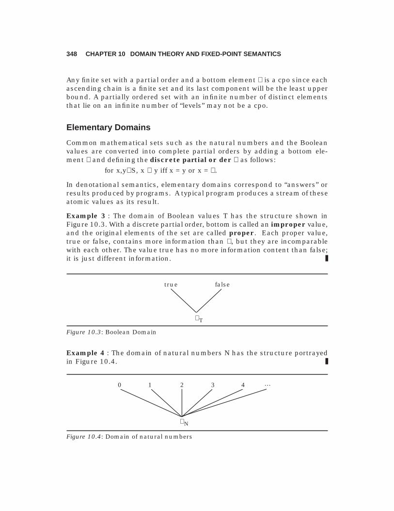
Any finite set with a partial order and a bottom element ⊥ is a cpo since eachascending chain is a finite set and its last component will be the least upperbound. A partially ordered set with an infinite number of distinct elementsthat lie on an infinite number of “levels” may not be a cpo.

Elementary Domains

Common mathematical sets such as the natural numbers and the Booleanvalues are converted into complete partial orders by adding a bottom ele-ment ⊥ and defining the discrete partial or der ⊆ as follows:

for x,y∈S, x ⊆ y iff x = y or x = ⊥.

In denotational semantics, elementary domains correspond to “answers” orresults produced by programs. A typical program produces a stream of theseatomic values as its result.

Example 3 : The domain of Boolean values T has the structure shown inFigure 10.3. With a discrete partial order, bottom is called an improper value,and the original elements of the set are called proper . Each proper value,true or false, contains more information than ⊥, but they are incomparablewith each other. The value true has no more information content than false;it is just different information. ❚

true false

⊥T

Figure 10.3: Boolean Domain

Example 4 : The domain of natural numbers N has the structure portrayedin Figure 10.4. ❚

0 1 2 3 …

⊥N

4

Figure 10.4: Domain of natural numbers

349

Do not confuse the “approximates” ordering ⊆ with the numeric ordering ≤on the natural numbers. Under ⊆, no pair of natural numbers is comparable,since neither contains more or even the same information as the other. Theseprimitive complete partially ordered sets are also called elementary or flatdomains . More complex domains are formed by three domain constructors.

Product Domains

Definition : If A with ordering ⊆A and B with ordering ⊆B are complete partialorders, the product domain of A and B is AxB with the ordering ⊆AxB where

AxB = {<a,b> | a∈A and b∈B} and

<a,b> ⊆AxB <c,d> iff a ⊆A c and b ⊆B d. ❚

It is a simple matter to show that ⊆AxB is a partial order on AxB, which weinvite the reader to try as an exercise. Assuming that a product domain is apartial order, we need a bottom element and least upper bound for ascendingchains to guarantee it is a cpo.

Theorem: ⊆AxB is a complete partial order on AxB.

Proof: ⊥AxB = <⊥A,⊥B> acts as bottom for AxB, since ⊥A ⊆A a and ⊥B ⊆ B b foreach a∈A and b∈B. If <a1,b1> ⊆ <a2,b2> ⊆ <a3,b3> ⊆ … is an ascending chainin AxB, then a1 ⊆A a2 ⊆A a3 ⊆A … is a chain in A with a least upper boundlub{ai|i≥1}∈A, and b1 ⊆B b2 ⊆B b3 ⊆B … is a chain in B with a least upperbound lub{bi|i≥1}∈B. Therefore lub{<ai,bi>|i≥1} = <lub{ai|i≥1},lub{bi|i≥1}>∈AxBis the least upper bound for the original chain. ❚

A product domain can be constructed with any finite set of domains in thesame manner. If D1, D2, …, Dn are domains (sets with complete partial or-ders), then D1xD2x…xDn with the induced partial order is a domain. If theoriginal domains are identical, then the product domain is written Dn.

Example 5 : Consider a classification of university students according to twodomains.

1. Level = {⊥L, undergraduate, graduate, nondegree}

2. Gender = {⊥G, female, male}

The product domain Level x Gender allows 12 different values as depicted inthe diagram in Figure 10.5, which shows the partial ordering between theelements using only the first letters to symbolize the values. Notice that sixvalues are “partial”, containing incomplete information for the classification.We can interpret these partial values by imagining two processes, one todetermine the level of a student and the other to ascertain the gender. Thesix incomplete values fit into one of three patterns.

10.2 DOMAIN THEORY


<⊥L,⊥G> Both processes fail to terminate normally.

<⊥L,male> The Gender process terminates with a result but the Levelprocess fails.

<graduate,⊥G> The Level process completes but the Gender one does notterminate normally. ❚

<u,f> <g,f> <n,f> <u,m> <g,m> <n,m>

<⊥L,f> <u,⊥G> <g,⊥G> <n,⊥G> <⊥L,m>

<⊥L,⊥G>

Figure 10.5: Level x Gender

To choose components from an element of a product domain, selector func-tions are defined on the structured domain.

Definition : Assume that for any product domain AxB, there are projectionfunctions

first : AxB→A, defined by first <a,b> = a for any <a,b>∈AxB, and

second : AxB→B, defined by second <a,b> = b for any <a,b>∈AxB. ❚

Selector functions of this sort may be applied to arbitrary product domains,D1xD2x…xDn. As a shorthand notation we sometimes use 1st, 2nd, 3rd, …,nth, for the names of the selector functions.

Example 6 : We used a product domain IntegerxOperationx IntegerxIntegerto represent the states of the calculator in Chapter 9. In the semantic equa-tions of Figure 9.8, pattern matching simulates the projection functions—for example, the equation

meaning [[P]] = d where (a,op,d,m) = perform [[P]] (0,nop,0,0)

abbreviates the equation

meaning [[P]] = third(perform [[P]] (0,nop,0,0)).

Similarly,

evaluate [[MR]] (a,op,d,m) = (a,op,m,m)

351

is a more readable translation of

evaluate [[MR]] st = (first(st),second(st),fourth(st),fourth(st)). ❚

Generally, using pattern matching to select components from a structureleads to more understandable definitions, as witnessed by its use in Prologand many functional programming languages, such as Standard ML.

Sum Domains (Disjoint Unions)

Definition : If A with ordering ⊆A and B with ordering ⊆B are complete partialorders, the sum domain of A and B is A+B with the ordering ⊆A+B defined by

A+B = {<a,1> | a∈A} ∪ {<b,2> | b∈B} ∪ {⊥A+B},

<a,1> ⊆A+B <c,1> if a ⊆A c,

<b,2> ⊆A+B <d,2> if b ⊆B d,

⊥A+B ⊆A+B <a,1> for each a∈A,

⊥A+B ⊆A+B <b,2> for each b∈B, and

⊥A+B ⊆A+B ⊥A+B. ❚

The choice of “1” and “2” as tags in a disjoint union is purely arbitrary. Anytwo distinguishable values can serve the purpose. In Chapter 9 we used thesymbols int and bool as tags for the sum domain of storable values whenspecifying the semantics of Wren,

SV = int(Integer) + bool(Boolean),

which can be thought of as an abbreviation of {<i,int>|i∈Integer} ∪{<b,bool>|b∈Boolean} ∪ {⊥}.

Again it is not difficult to show that ⊆A+B is a partial order on A+B, and theproof is left as an exercise.

Theorem: ⊆A+B is a complete partial order on A+B.

Proof: ⊥A+B ⊆ x for any x∈A+B by definition. An ascending chain x1 ⊆ x2 ⊆ x3⊆ … in A+B may repeat ⊥A+B forever or eventually climb into either Ax{1} orBx{2}. In the first case, the least upper bound will be ⊥A+B, and in the othertwo cases the least upper bound will exist in A or B. ❚

Example 7 : The sum domain T+N (Boolean values and natural numbers)may be viewed as the structure portrayed in Figure 10.6, where the tags havebeen omitted to simplify the diagram. ❚

10.2 DOMAIN THEORY


⊥T+N

0 1 2 3 …

⊥N

4true false

⊥T

Figure 10.6: The sum domain T+N

A sum domain can be constructed with any finite set of domains in the samemanner as with two domains. If D1, D2, …, Dn are domains (sets with com-plete partial orders), then D1 + D2 + … + Dn = {<d,i> | d∈Di, 1≤i≤n} ∪ {⊥}withthe induced partial order is a domain.

Functions on sum domains include a constructor, a selector, and a testingfunction.

Definition : Let S = A+B, where A and B are two domains.

1. Injection (creation):

inS : A→S is defined for a∈A as inS a = <a,1>∈S

inS : B→S is defined for b∈B as inS b = <b,2>∈S

2. Projection (selection):

outA : S→A is defined for s∈S as outA s = a∈A if s=<a,1>, andoutA s = ⊥A∈A if s=<b,2> or s=⊥S.

outB : S→B is defined for s∈S as outB s = b∈B if s=<b,2>, andoutB s = ⊥B∈B if s=<a,1> or s=⊥S.

3. Inspection (testing): Recall that T = {true, false, ⊥T}.

isA : S→T is defined for s∈S as(isA s) if and only if there exists a∈A with s=<a,1>.

isB : S→T is defined for s∈S as(isB s) if and only if there exists b∈B with s=<b,2>.

In both cases, ⊥S is mapped to ⊥T. ❚

Example 8 : In the semantic domain of storable values for Wren shown inFigure 9.10, the identifiers int and bool act as the tags to specify the separatesets of integers and Boolean values. The notation

353

SV = int(Integer) + bool(Boolean)= {int(n)|n∈Integer} ∪ {bool(b)|b∈Boolean} ∪ {⊥SV}

represents the sum domain

SV = (Integer x {int}) ∪ (Boolean x {bool}) ∪ {⊥SV}.

Then an injection function is defined by

inSV : Integer → SV where inSV n = int(n). ❚

Actually, the tags themselves can be thought of as constituting the injectionfunction (or as constructors) with the syntax int : Integer → SV andbool : Boolean → SV, so that we can dispense with the special injection func-tion inSV.

A projection function takes the form

outInteger : SV → Integer where outInteger int(n) = noutInteger bool(b) = ⊥.

Inspection is handled by pattern matching, as in the semantic equation

execute [[if E then C]] sto = if p then execute [[C]] sto else stowhere bool(p) = evaluate [[E]] sto,

which stands for

execute [[if E then C]] sto =if isBoolean(val)

then if outBoolean(val) then execute [[C]] sto else stoelse ⊥

where val = evaluate [[E]] sto.

Example 9 : In the sum domain Level + Gender shown in Figure 10.7, tags lvfor level and gd for gender are attached to the elements from the two compo-nent domains. If a computation attempts to identify either the level or thegender of a particular student (but not both), it may utterly fail giving ⊥, itmay be able to identify the level or the gender of the student, or as a middleground it may know that the computation is working on the level value butmay not be able to complete its work, thus producing the result ⊥L. ❚

An infinite sum domain may be defined in a similar way.If D1, D2, D3, … are domains, then D1 + D2 + D3 + … contains elements of theform <d,i> where d∈Di for i≥1 plus a new bottom element.

This infinite sum domain construction allows the definition of the domain ofall finite sequences (lists) formed using elements from a domain D and de-noted by D*.

10.2 DOMAIN THEORY


lv (undergraduate)

lv (⊥L)

⊥ L+G

gd (⊥G)

lv (graduate)

lv (nondegree) gd (female) gd (male)

Figure 10.7: Level + Gender

D* = {nil }+D+D2+D3+D4+… where nil represents the empty sequence.

An element of D* is either the empty list nil, a finite ordered tuple from Dk forsome k≥1, or ⊥.

Special selector and constructor functions are defined on D*.

Definition : Let L∈D* and e∈D. Then L=<d,k> for d∈Dk for some k≥0 whereD0 = {nil }.

1. head : D*→D wherehead (L) = first (outDk(L)) if k>0 and head (<nil,0>) = ⊥.

2. tail : D*→D* wheretail (L) = inD* (<2nd(outDk(L)),3rd(outDk(L)),…,kth(outDk(L))>) if k>0 andtail (<nil,0>) = ⊥.

3. null : D*→T wherenull (<nil,0>) = true and null (L) = false if L = <d,k> with k>0.Therefore null (L) = isD0(L).

4. prefix : DxD*→D* whereprefix (e,L) = inD* (<e,1st(outDk(L)),2nd(outDk(L)),…,kth(outDk(L))>) andprefix (e,<nil,0>)) = <<e>,1>

5. affix : D*xD→D* whereaffix (L,e) = inD* (<1st(outDk(L)),2nd(outDk(L)),…,kth(outDk(L)),e>) andaffix (<nil,0>,e) = <<e>,1>. ❚

Each of these five functions on lists maps bottom to bottom. The binaryfunctions prefix and affix produce ⊥ if either argument is bottom.

355

Function Domains

Definition : A function from a set A to a set B is total if f(x)∈B is defined forevery x∈A. If A with ordering ⊆A and B with ordering ⊆B are complete partialorders, define Fun(A,B) to be the set of all total functions from A to B. (Thisset of functions will be restricted later.) Define ⊆ on Fun(A,B) as follows:

For f,g∈Fun(A,B), f ⊆ g if f(x) ⊆B g(x) for all x∈A. ❚

Lemma : ⊆ is a partial order on Fun(A,B).

Proof:1. Reflexive: Since ⊆B is reflexive, f(x) ⊆B f(x) for all x∈A, so f ⊆ f for any

f∈Fun(A,B).

2. Transitive: Suppose f ⊆ g and g ⊆ h. Then f(x) ⊆B g(x) and g(x) ⊆B h(x) forall x∈A. Since ⊆B is transitive, f(x) ⊆B h(x) for all x∈A, and so f ⊆ h.

3. Antisymmetric: Suppose f ⊆ g and g ⊆ f. Then f(x) ⊆B g(x) and g(x) ⊆Bf(x) for all x∈A. Since ⊆B is antisymmetric, f(x) = g(x) for all x∈A, and sof = g. ❚

Theorem: ⊆ is a complete partial order on Fun(A,B).

Proof: Define bottom for Fun(A,B) as the function ⊥(x) = ⊥B for all x∈A. Since⊥(x) = ⊥B ⊆B f(x) for all x∈A and f∈Fun(A,B), ⊥ ⊆ f for any f∈Fun(A,B). Let f1 ⊆f2 ⊆ f3 ⊆ … be an ascending chain in Fun(A,B). Then for any x∈A, f1(x) ⊆B f2(x)⊆B f3(x) ⊆B … is a chain in B, which has a least upper bound, yx∈B. Note thatyx is lub{fi(x)|i≥1}. Define the function F(x) = yx for each x∈A. F serves as aleast upper bound for the original chain. Set lub{fi|i≥1} = F. ❚

The set Fun(A,B) of all total functions from A to B contains many functionswith abnormal behavior that precludes calculating or even approximatingthem on a computer. For example, consider a function H : (N→N) → (N→N)defined by

for g∈N→N, H g = λn . if g(n)=⊥ then 0 else 1.

Certainly H∈Fun(N→N,N→N), but if we make this function acceptable in thedomain theory that provides a foundation for denotational definitions, wehave accepted a function that solves the halting problem—that is, whetheran arbitrary function halts normally on given data. To exclude this and otherabnormal functions, we place two restrictions on functions to ensure thatthey have agreeable behavior.

Definition : A function f in Fun(A,B) is monotonic if x ⊆A y implies f(x) ⊆B f(y)for all x,y∈A. ❚

Since we interpret ⊆ to mean “approximates”, whenever y has at least asmuch information as x, it follows that f(y) has at least as much information

10.2 DOMAIN THEORY


as f(x). We get more information out of a function by putting more informa-tion into it.

An ascending chain in a partially order set can be viewed as a subset of thepartially ordered set on which the ordering is total (any two elements arecomparable).

Definition : A function f∈Fun(A,B) is continuous if it preserves least upperbounds—that is, if x1 ⊆A x2 ⊆A x3 ⊆A … is an ascending chain in A, thenf(lub{xi|i≥1}}) = lub{f(xi)|i≥1}. ❚

Note that if f is also monotonic, then f(x1) ⊆B f(x2) ⊆B f(x3) ⊆B … is an ascend-ing chain. Intuitively, continuity means that there are no surprises whentaking the least upper bounds (limits) of approximations. The diagram inFigure 10.8 shows the relation between the two chains.

x1 ⊆A x2 ⊆A x3 ⊆A … ⇒ lub{xi|i≥1}

↓ ↓ ↓ ↓f(x1) ⊆B f(x2) ⊆B f(x3) ⊆B … ⇒ lub{f(xi)|i≥1} = f(lub{xi|i≥1})

Figure 10.8: Continuity

A continuous function f has predictable behavior in the sense that if we knowits value on the terms of an ascending chain x1 ⊆ x2 ⊆ x3 ⊆ …, we also knowits value on the least upper bound of the chain since f(lub{xi|i≥1}) is the leastupper bound of the chain f(x1) ⊆ f(x2) ⊆ f(x3) ⊆ …. It is possible to predict thevalue of f on lub{xi|i≥1} by its behavior on each xi.

Lemma : If f∈Fun(A,B) is continuous, it is also monotonic.

Proof: Suppose f is continuous and x ⊆A y. Then x ⊆A y ⊆A y ⊆A y ⊆A … is anascending chain in A, and so by the continuity of f,

f(x) ⊆B lubB{f(x),f(y)} = f(lubA{x,y}) = f(y). ❚

Definition : Define A→B to be the set of functions in Fun(A,B) that are(monotonic and) continuous. This set is ordered by the relation ⊆ fromFun(A,B). ❚

Lemma : The relation ⊆ restricted to A→B is a partial order.

Proof: The properties reflexive, transitive, and antisymmetric are inheritedby a subset. ❚

The example function H : (N→N) → (N→N) defined by

for g∈N→N, H g = λn . if g(n)=⊥ then 0 else 1

is neither monotonic nor continuous. It suffices to show that it is not mono-tonic by a counterexample.

357

Let g1 = λn . ⊥ and g2 = λn . 0. Then g1 ⊆ g2. But H(g1) = λn . 0, H(g2) = λn . 1,and the functions λn . 0 and λn . 1 are not related by ⊆ at all.

Two lemmas will be useful in proving the continuity of functions.

Lub Lemma : If x1 ⊆ x2 ⊆ x3 ⊆ … is an ascending chain in a cpo A, and xi ⊆d∈A for each i≥1, it follows that lub{xi|i≥1} ⊆ d.

Proof: By the definition of least upper bound, if d is a bound for the chain, theleast upper bound lub{xi|i≥1} must be no larger than d. ❚

Limit Lemma : If x1 ⊆ x2 ⊆ x3 ⊆ … and y1 ⊆ y2 ⊆ y3 ⊆ … are ascending chainsin a cpo A, and xi ⊆ yi for each i≥1, then lub{xi|i≥1} ⊆ lub{yi|i≥1}.

Proof: For each i≥1, xi ⊆ yi ⊆ lub{yi|i≥1}. Therefore lub{xi|i≥1} ⊆ lub{yi|i≥1} bythe Lub lemma (take d = lub{yi|i≥1}). ❚

Theorem: The relation ⊆ on A→B, the set of functions in Fun(A,B) that aremonotonic and continuous, is a complete partial order.

Proof: Since ⊆ is a partial order on A→B, two properties need to be verified.

1. The bottom element in Fun(A,B) is also in A→B, which can be proved byshowing that the function ⊥(x) = ⊥B is monotonic and continuous.

2. For any ascending chain in A→B, its least upper bound, which is an ele-ment of Fun(A,B), is also in A→B, which means that it is monotonic andcontinuous.

Part 1 : If x ⊆A y for some x,y∈A, then ⊥(x) = ⊥B = ⊥(y), which means ⊥(x) ⊆B⊥(y), and so ⊥ is a monotonic function. If x1 ⊆A x2 ⊆A x3 ⊆A … is an ascendingchain in A, then its image under the function ⊥ will be the ascending chain⊥B ⊆B ⊥B ⊆B ⊥B ⊆B …, whose least upper bound is ⊥B. Therefore ⊥(lub{xi|i≥1})= ⊥B = lub{⊥(xi)|i≥1}, and ⊥ is a continuous function.

Part 2 : Let f1 ⊆ f2 ⊆ f3 ⊆ … be an ascending chain in A→B, and let F =lub{fi|i≥1} be its least upper bound (in Fun(A,B)). Remember the definition ofF, F(x) = lub{fi(x)|i≥1} for each x∈A. We need to show that F is monotonic andcontinuous so that we know F is a member of A→B.

Monotonic : If x ⊆A y, then fi(x) ⊆B fi(y) ⊆B lub{fi(y)|i≥1} for any i since each fiis monotonic. Therefore F(y) = lub{fi(y)|i≥1} is an upper bound for each fi(x),and so the least upper bound of all the fi(x) satisfies F(x) = lub{fi(x)|i≥1} ⊆ F(y),and F is monotonic. This result can also be proved using the Limit lemma.Since fi(x) ⊆B fi(y) for each i≥1, F(x) = lub{fi(x)|i≥1} ⊆ lub{fi(y)|i≥1} = F(y).

10.2 DOMAIN THEORY


Continuous : Let x1 ⊆A x2 ⊆A x3 ⊆A … be an ascending chain in A. We need toshow that F(lub{xj|j≥1}) = lub{F(xj)|j≥1} where F(x) = lub{fi(x)|i≥1} for eachx∈A. Note that “i” is used to index the ascending chain of functions fromA→B while “j” is used to index the ascending chains of elements in A and B.So F is continuous if F(lub{xj|j≥1}) = lub{F(xj)|j≥1}.

Recall these definitions and properties.

1. Each fi is continuous: fi(lub{xj|j≥1}) = lub{fi(xj)|j≥1} for each chain {xj|j≥1}in A.

2. Definition of F: F(x) = lub{fi(x)|i≥1} for each x∈A.

Thus F(lub{xj|j≥1}) = lub{fi(lub{xj|j≥1})|i≥1} by 2= lub{lub{fi(xj)|j≥1}|i≥1} by 1= lub{lub{fi(xj)|i≥1}|j≥1} ‡ needs to be shown= lub{F(xj)|j≥1} by 2.

The condition ‡ to be proved is illustrated in Figure 10.9.

f1(x1) ⊆ f2(x1) ⊆ f3(x1) ⊆ F(x1)

f1(x2) ⊆ f2(x2) ⊆ f3(x2) ⊆ F(x2)

f1(x3) ⊆ f2(x3) ⊆ f3(x3) ⊆ F(x3)

f1(lub {xj|j≥1}) ⊆ f2(lub {xj|j≥1}) ⊆ f3(lub {xj|j≥1}) ⊆ ?

⊆ ⊆ ⊆

⊆

⊆⊆

⊆ ⊆ ⊆⊆⊆⊆

⊆⊆

⊆

⊆ ⊆ ⊆

lub {xj|j≥1}

x3

x1

x2

f1 f2 f3 F=lub {fi|i≥1}

Figure 10.9: Continuity of F = lub{fi|i≥1}

The rows in the diagram correspond to the definition of F as the least upperbound of the ascending chain of functions lub{fi|i≥1}. The columns corre-spond to the continuity of each fi—namely, that lub{fi(xj)|j≥1} = fi(lub{xj|j≥1})for each i and each ascending chain {xj|j≥1} in A.

35910.2 DOMAIN THEORY

First Half : lub{lub{fi(xj)|j≥1}|i≥1} ⊆ lub{lub{fi(xj)|i≥1}|j≥1}

For all k and j, fk(xj) ⊆ lub{fi(xj)|i≥1} by the definition of F (the rows ofFigure 10.9). We have ascending chains fk(x1) ⊆ fk(x2) ⊆ fk(x3) ⊆ … foreach k and lub{fi(x1)|i≥1} ⊆ lub{fi(x2)|i≥1} ⊆ lub{fi(x3)|i≥1} ⊆ …. So for eachk, lub{fk(xj)|j≥1} ⊆ lub{lub{fi(xj)|i≥1}|j≥1} by the Limit lemma. This corre-sponds to the top row. Hence lub { lub { fk(x j)|j≥1}|k≥1} ⊆lub{lub{fi(xj)|i≥1}|j≥1} by the Lub lemma. Now change k to i.

Second Half : lub{lub{fi(xj)|i≥1}|j≥1} ⊆ lub{lub{fi(xj)|j≥1}|i≥1}

For all i and k, fi(xk) ⊆ fi(lub{xj|j≥1}) = lub{fi(xj)|j≥1} by using the fact that eachfi is monotonic and continuous (the columns of Figure 10.9). So for each k,lub{fi(xk)|i≥1} ⊆ lub{lub{fi(xj)|j≥1}|i≥1} by the Limit lemma. This correspondsto the rightmost column. Hence lub{lub{fi(xk)|i≥1}|k≥1} ⊆ lub{lub {fi(xj)|j≥1}|i≥1}by the Lub lemma. Now change k to j.

Therefore F is continuous. ❚

Corollary : Let f1 ⊆ f2 ⊆ f3 ⊆ … be an ascending chain of continuous functionsin A→B. Then F = lub{fi|i≥1} is a continuous function.

Proof: This corollary was proved in Part 2 of the proof of the previous theo-rem. ❚

In agreement with the notation for denotational semantics in Chapter 9, as adomain constructor, we treat → as a right associative operation. The domainA→B→C means A→(B→C), which is the set of continuous functions from Ainto the set of continuous functions from B to C. If f∈A→B→C, then for a∈A,f(a)∈B→C. Generally, we write “:” to represent membership in a domain. Sowe write g : A→B for g∈A→B.

Example 10 : Consider the functions from a small domain of students,

Student = {⊥, Autry, Bates}

to the domain of levels,

Level = {⊥, undergraduate, graduate, nondegree}.

We can think of the functions in Fun(Student,Level) as descriptions of oursuccess in classifying two students, Autry and Bates. The set of all totalfunctions, Fun(Student,Level), contains 64 (43) elements, but only 19 of thesefunctions are monotonic and continuous. The structure of Student → Levelis portrayed by the lattice-like structure in Figure 10.10, where the values inthe domains are denoted by only their first letters. ❚

Since the domain Student of a function in Student→Level is finite, it is enoughto show that the function is monotonic as we show in the next theorem.


a → ub → u⊥ → u

a → gb → g⊥ → g

a → nb → n⊥ → n

a → gb → n⊥ → ⊥

a → nb → g⊥ → ⊥

a → nb → n⊥ → ⊥

a → ub → u⊥ → ⊥

a → nb → u⊥ → ⊥

a → ub → g⊥ → ⊥

a → ub → ⊥⊥ → ⊥

a → gb → g⊥ → ⊥

a → ub → n⊥ → ⊥

a → gb → u⊥ → ⊥

a → gb → ⊥⊥ → ⊥

a → nb → ⊥⊥ → ⊥

a →⊥b → g⊥ → ⊥

a → ⊥b → n⊥ → ⊥

a → ⊥b → u⊥ → ⊥

a → ⊥b → ⊥⊥ → ⊥

Figure 10.10: Function domain Student → Level

Theorem: If A and B are cpo’s, A is a finite set, and f∈Fun(A,B) is monotonic,then f is also continuous.

Proof: Let x1 ⊆A x2 ⊆A x3 ⊆A … be an ascending chain in A. Since A is finite, forsome k, xk = xk+1 = xk+2 = …. So the chain is a finite set {x1, x2, x3, …, xk}whose least upper bound is xk. Since f is monotonic, f(x1) ⊆B f(x2) ⊆B f(x3) ⊆B

361

… ⊆B f(xk) = f(xk+1) = f(xk+2) = … is an ascending chain in B, which is also afinite set—namely, {f(x1), f(x2), f(x3), …, f(xk)} with f(xk) as its least upper bound.Therefore, f(lub{xi|i≥1}) = f(xk) = lub{f(xi)|i≥1}, and f is continuous. ❚

Lemma : The function f : Student → Level defined by

f(⊥) = graduate, f(Autry) = nondegree, f(Bates) = graduate

is neither monotonic nor continuous.

Proof: Clearly, ⊥ ⊆ Autry. But f(⊥) = graduate and f(Autry) = nondegree areincomparable. Therefore, f is not monotonic. By the contrapositive of an ear-lier theorem, if f is not monotonic, it is also not continuous. ❚

Continuity of Functions on Domains

The notation used for the special functions defined on domains implied thatthey were continuous—for example, first : AxB→A. To justify this notation, atheorem is needed.

Theorem: The following functions on domains and their analogs are con-tinuous:

1. first : AxB→A

2. inS : A→S where S = A+B

3. outA : A+B→A

4. isA : A+B→T

Proof:1. Let <a1,b1> ⊆ <a2,b2> ⊆ <a3,b3> ⊆ … be an ascending chain in AxB.

Then lub{first <ai,bi>|i≥1} = lub{ai|i≥1}= first <lub{ai|i≥1},lub{bi|i≥1}> = first (lubAxB{<ai,bi>|i≥1}).

2. An exercise.

3. An exercise.

4. An ascending chain x1 ⊆ x2 ⊆ x3 ⊆ … in A+B may repeat ⊥A+B forever oreventually climb into either Ax{1} or Bx{2}. In the first case, the least up-per bound will be ⊥A+B, and in the other two cases the lub will be somea∈A or some b∈B.

Case 1 : {xi|i≥1} = {⊥A+B}. Then isA(lubA+B{xi|i≥1}) = isA(⊥A+B) = ⊥T, andlubT{isA(xi)|i≥1} = lubT{isA(⊥A+B)} = lubT{⊥T} = ⊥T.

Case 2 : {xi|i≥1} = {⊥A+B,…,⊥A+B,<a1,1>,<a2,1>,…} where a1 ⊆A a2 ⊆A a3⊆A … is a chain in A. Suppose a = lub{ai|i≥1}. Then isA(lubA+B{xi|i≥1}) =isA(<a,1>) = true, and lubT{isA(xi)|i≥1} = lubT{⊥,…,⊥,true,true,…} = true.

10.2 DOMAIN THEORY


Case 3 : {xi|i≥1} = {⊥A+B,…,⊥A+B,<b1,2>,<b2,2>,…} where b1 ⊆B b2 ⊆B b3⊆B … is a chain in B. Suppose b = lub{bi|i≥1}.Then isA(lubA+B{xi|i≥1}) =isA(<b,2>) = false, and lubT{isA(xi)|i≥1} = lubT{⊥,…,⊥,false,false,…} =false. ❚

The functions defined on lists, such as head and tail, are mostly built fromthe selector functions for products and sums. The list functions can be shownto be continuous by proving that composition preserves the continuity offunctions.

Theorem: The composition of continuous functions is continuous.

Proof: Suppose f : A → B and g : B → C are continuous functions. Let a1 ⊆ a2⊆ a3 ⊆ … be an ascending chain in A. Then f(a1) ⊆ f(a2) ⊆ f(a3) ⊆ … is anascending chain in B with f(lub{ai|i≥1}) = lub{f(ai)|i≥1} by the continuity of f.Since g is continuous, g(f(a1)) ⊆ g(f(a2)) ⊆ g(f(a3)) ⊆ … is an ascending chain inC with g(lub{f(ai)|i≥1}) = lub{g(f(ai))|i≥1}. Therefore g(f(lub{ai|i≥1})) =g(lub{f(ai)|i≥1}) = lub{g(f(ai))|i≥1} and g°f is continuous. ❚

To handle tail, prefix, and affix we need a generalization of this theorem to allowfor tuples of continuous functions, a result that appears as an exercise.

Theorem: The following functions on lists are continuous:

1. head : D* → D2. tail : D*→ D*

3. null : D* → T4. prefix : DxD* → D*

5. affix : D*xD → D*

Proof: For 1, 2, 4, 5 use the continuity of the compositions of continuousfunctions and the previous theorems. A case analysis is needed to deal withascending sequences that contain mostly nil values.

3. An ascending chain x1 ⊆ x2 ⊆ x3 ⊆ … in D* may repeat ⊥D* forever oreventually climb into Dk, where k≥0 and D0 = {nil }.

Case 1 : {xi|i≥1} = {⊥D*}. null(lubD*{xi|i≥1}) = null(⊥D*) = ⊥T, andlubT{null(xi)|i≥1} = lubT{⊥T} = ⊥T.

Case 2 : {xi|i≥1} = {⊥D*,⊥D*,…,⊥D*,<nil,0>,<nil,0>,…}.null(lubD*{xi|i≥1}) = null(<nil,0>) = true, andlubT{null(xi)|i≥1} = lubT{⊥T,⊥T,…,⊥T,true,true,…} = true.

Case 3 : {xi|i≥1} = {⊥D*,…,⊥D*,<d1,k>,<d2,k>,…} where di∈Dk for some k>0and d1 ⊆Dk d2 ⊆Dk d3 ⊆Dk … is a chain in Dk. null(lubD*{xi|i≥1}) =null(<lubDk{di|i≥1},k>) = false since (lubDk{di|i≥1})∈Dk, and lubD{null(xi)|i≥1}= lubD{null<d1,k>, null<d2,k>, …} = lubD{false, false, …} = false. ❚

36310.2 DOMAIN THEORY

Exercises

1. Determine which of the following ordered sets are complete partial orders:

a) Divides ordering on {1,3,6,9,12,18}.

b) Divides ordering on {2,3,6,12,18}.

c) Divides ordering on {2,4,6,8,10,12}.

d) Divides ordering on the set of positive integers.

e) Divides ordering on the set P of prime numbers.

f) Divides ordering on the set P ∪ {1}.

g) ⊆ (subset) on the nonempty subsets of {a,b,c,d}.

h) ⊆ (subset) on the collection of all finite subsets of the natural num-bers.

i) ⊆ (subset) on the collection of all subsets of the natural numberswhose complement is finite.

2. Which of the partially ordered sets in exercise 1 are also lattices?

3. Let S = {1,2,3,4,5,6,9,15,25,30} be ordered by the divides relation.

a) Find all lower bounds for {6,30}.

b) Find all lower bounds for {4,6,15}.

c) Find all upper bounds for {1,2,3}.

d) Does {4,9,25} have an upper bound?

4. Show that ⊆AxB is a partial order on AxB.

5. Show that ⊆A+B is a partial order on A+B.

6. Prove that the least upper bound of an ascending chain x1 ⊆ x2 ⊆ x3 ⊆ …in a domain D is unique.

7. Let Hair = {⊥,black,blond,brown} and Eyes = {⊥,blue,brown,gray} be twoelementary domains (flat complete partially ordered sets).

a) Sketch a Hasse diagram showing all the elements of Hair x Eyes andthe relationships between its elements under ⊆.

b) Sketch a Hasse diagram showing all the elements of Hair+Eyes andthe relationships between its elements under ⊆.


8. Suppose that A = {⊥,a} and B = {⊥,b,c,d} are elementary domains.

a) Sketch a Hasse diagram showing all seven elements of A→B and therelationships between its elements under ⊆.

b) Give an example of one function in Fun(A,B) that is not monotonic.

c) Sketch a Hasse diagram showing all the elements of AxB and therelationships between its elements under ⊆.

9. Suppose A = {⊥,a,b} and B = {⊥,c} are elementary domains.

a) Sketch a Hasse diagram showing all the elements of (A→B)+(AxB) andtheir ordering under the induced partial order. Represent functionsas sets of ordered pairs. Since A→B and AxB are disjoint, omit thetags on the elements, but provide subscripts for the bottom elements.

b) Give one example of a function in Fun(A→B,AxB) that is continuousand one that is not monotonic.

10. Prove the following property:

A function f in Fun(A,B) is continuous if and only if both of the followingconditions hold.

a) f is monotonic.

b) For any ascending chain x1 ⊆ x2 ⊆ x3 ⊆ … in A, f(lubA{xi|i≥1}) ⊆lubB{f(xi)|i≥1}.

11. Let A = {⊥,a1,a2,…,am} and B = {⊥,b1,b2,…,bn} be flat domains. Show that

a) Fun(A,B) has (n+1)m+1 elements.

b) A→B has n+(n+1)m elements.

12. Prove that inS and outA are continuous functions.

13. Prove that head and tail are continuous functions.

14. Tell whether these functions F : (N→N)→(N→N) are monotonic and/orcontinuous.

a) F g n = if total(g) then g(n) else ⊥, where total(g) is true if and only ifg(n) is defined (not ⊥) for all proper n∈N.

b) F g n = if g = (λn .0) then 1 else 0.

c) F g n = if n∉dom(g) then 0 else ⊥, where dom(g) ={n∈N | g(n)≠⊥}denotes the domain of g.

365

15. Let N = {⊥,0,1,2,3,…} be the elementary domain of natural numbers. Afunction f : N→N is called strict if f(⊥) = ⊥. Consider the function add1 :N→N defined by add1(n) = n+1 for all n∈N with n≠⊥. Prove that if add1 ismonotonic, it must also be strict.

16. Consider the function F : (N→N) → (N→N) defined by

for g∈N→N, F g = λn . if g(n)=⊥ then 0 else 1

Describe F g1, F g2, and F g3 where the gk : N→N are defined by

g1(n) = n

g2(n) = if n>0 then n/0 else ⊥

g3(n) = if even(n) then n+1 else ⊥

17. Prove that if f∈Fun(A,B), where A and B are domains (cpo’s), is a con-stant function (there is a b∈B such that f(a) = b for all a∈A), then f iscontinuous.

18. An ascending chain x1 ⊆ x2 ⊆ x3 ⊆ … in a cpo A is called stationary ifthere is an n≥1 such that for all i≥n, xi = xn. Carefully prove the followingproperties:

a) If every ascending chain in A is stationary and f∈Fun(A,B) is mono-tonic, then f must be continuous.

b) If an ascending chain x1 ⊆ x2 ⊆ x3 ⊆ … is not stationary, then for alli≥1, xi ≠ lub{xj|j≥1}. Hint: Prove the contrapositive.

19. Prove the following lemma: If a1 ⊆ a2 ⊆ a3 ⊆ … and b1 ⊆ b2 ⊆ b3 ⊆ … areascending chains with the property that for each m≥1 there exists ann≥1 such that am ⊆ bn, it follows that lub{ai|i≥1} ⊆ lub{bi|i≥1}.

10.3 FIXED-POINT SEMANTICS

Functions, and in particular recursively defined functions, are central to com-puter science. Functions are used not only in programming but also in de-scribing the semantics of programming languages as witnessed by the recur-sive definitions in denotational specifications. Recursion definitions entail acircularity that can make them suspect. Many of the paradoxes of logic andmathematics revolve about circular definitions—for example, the set of allsets. Considering the suspicious nature of circular definitions, how can webe certain that function definitions have a consistent model? The use of do-mains (complete partially ordered sets) and the associated fixed-point theory



to be developed below put recursive function definitions and denotationalsemantics on a firm, consistent foundation.

Our goal is to develop a coherent theory of functions that makes sense out ofrecursive definitions. In describing fixed-point semantics we restate some ofthe definitions from section 10.2 as we motivate the concepts. The discus-sion breaks into two parts: (1) interpreting partial functions so that they aretotal, and (2) giving meaning to a recursively defined function as an approxi-mation of a sequence of “finite” functions.

First Step

We transform partial functions into analogous total functions.

Example 11 : Let f be a function on a few natural numbers with domain D ={0,1,2} and codomain C = {0,1,2} and with its rule given as

f(n) = 2/n or as a set of ordered pairs: f = {<1,2>,<2,1>}.

Note that f(0) is undefined; therefore f is a partial function. Now extend f tomake it a total function.

f = {<0,?>,<1,2>,<2,1>}.

Add an undefined element to the codomain, C+ = {⊥C+,0,1,2}, and for symme-try, do likewise with the domain, D+ = {⊥D+,0,1,2}.

Then define the natural extension of f by having ⊥D+ map to ⊥C+ under f.

f+ = {<⊥,⊥>,<0,⊥>,<1,2>,<2,1>}.

From this point on, we drop the subscripts on ⊥ unless they are neededto clarify an example. Finally, define a relationship that orders functionsand domains according to how “defined” they are, putting a lattice-likestructure on the elementary domains: For x,y∈D+, x⊆y if x=⊥ or x=y. Itfollows that f⊆f+. ❚

This relation is read “f approximates f+” or “f is less defined than or equal tof+”. D+ and C+ are examples of the flat domains of the previous section.

Consider the function g = {<⊥,⊥>,<0,0>,<1,2>,<2,1>}, which is an extensionof f+ that is slightly more defined. The relationship between the two functionsis denoted by f+ ⊆ g. Observe that the two functions agree where they areboth defined (do not map to ⊥).

Theorem: Let f+ be a natural extension of a function between two sets D andC so that f+ is a total function from D+ to C+. Then f+ is monotonic andcontinuous.

367

Proof: Let x1 ⊆ x2 ⊆ x3 ⊆ … be an ascending chain in the domain D+ = D∪{⊥D+}.There are two possibilities for the behavior of the chain.

Case 1 : xi = ⊥D+ for all i≥1. Then lub{xi|i≥1} = ⊥D+, and f+(lub{xi|i≥1}) = f+(⊥D+)= ⊥C+ = lub{⊥C+} = lub{f+(xi)|i≥1}.

Case 2 : xi = ⊥D+ for 1≤i≤k and ⊥D+ ≠ xk+1 = xk+2 = xk+3 = …, since once theterms move above bottom, the sequence is constant in a flat domain. Thenlub{xi|i≥1} = xk+1, and f+(lub{xi|i≥1}) = f+(xk+1) = lub{⊥C+,f+(xk+1)} = lub{f+(xi)|i≥1}.If f+ is continuous, it is also monotonic. ❚

Since many functions used in programming, such as “addition”, “less than”,and “or”, are binary operations, their natural extensions need to be clarified.

Definition : The natural extension of a function whose domain is a Carte-sian product—namely, f : D1

+xD2+x…xDn

+→C+—has the property thatf+(x1,x2,…,xn) = ⊥C whenever at least one xi=⊥. Any function that satisfies thisproperty is known as a strict function. ❚

Theorem: If f+: D1+xD2

+x…xDn+→C+ is a natural extension where Di

+, 1≤i≤n,and C+ are elementary domains, then f+ is monotonic and continuous.

Proof: Consider the case where n=2. We show f+ is continuous.Let <x1,y1> ⊆ <x2,y2> ⊆ <x3,y3> ⊆ … be an ascending chain in D1

+xD2+. Since

D1+ and D2

+ are elementary domains, the chains {xi|i≥1} and {yi|i≥1} mustfollow one of the two cases in the previous proof—namely, all ⊥ or eventuallyconstant proper values in D1

+ and D2+, respectively.

Case 1 : lub{xi|i≥1} = ⊥D1+ or lub{yi|i≥1} = ⊥D2

+ (or both). Then f+(lub{<xi,yi>|i≥1})= f+(<lub{xi|i≥1},lub{yi|i≥1}>) = ⊥C because f+ is a natural extension and oneof its arguments is ⊥; furthermore, lub{f+(<xi,yi>)|i≥1}= lub{⊥C+} = ⊥C+, sinceat least one of the chains must be all ⊥.

Case 2 : lub{xi|i≥1} = x∈D1 and lub{yi|i≥1} = y∈D2 (neither is ⊥). Since D1+

and D2+ are both elementary domains, there is an integer k such that xi = x

and yi = y for all i≥k. So f+(lub{<xi,yi>|i≥1}) = f+(<lub{xi|i≥1},lub{yi|i≥1}>) =f+(<x,y>)∈C+ and lub{f+(<xi,yi>)|i≥1}= lub{⊥C+,f+(<x,y>)} = f+(<x,y>). ❚

Example 12 : Consider the natural extension of the conditional expressionoperation (if a b c) = if a then b else c.

The natural extension unduly restricts the meaning of the conditional ex-pression—for example, we prefer that the following expression returns 0 whenm=1 and n=0 instead of causing a fatal error: if n>0 then m/n else 0.

But if we interpret the undefined operation 1/0 as ⊥, when m=1 and n=0,

(if+ n>0 m/n 0) = (if+ false ⊥ 0) = ⊥ for a natural extension. ❚



As we continue with the development of fixed-point semantics, we drop thesuperscript plus sign (+) on sets and functions since all sets will be assumedto be domains (cpo’s) and all functions will be naturally extended unlessotherwise specified.

Second Step

We now define the meaning of a recursive definition of a function defined oncomplete partially ordered sets (domains) as the limit of a sequence of ap-proximations.

Example 13 : Consider a recursively defined function f : N→N where N ={⊥,0,1,2,3,…} and

f(n) = if n=0 then 5 else if n=1 then f(n+2) else f(n-2). (†)

Two questions can be asked about a recursive definition of a function.

1. What function, if any, does this equation in f denote?

2. If the equation specifies more than one function, which one should beselected?

Define a functional F, a function on functions, by

F : (N→N)→(N→N) where(F(f)) (n) = if n=0 then 5 else if n=1 then f(n+2) else f(n-2). (‡)

Assuming function application associates to the left, we usually omit theparentheses with multiple applications, writing F f n for (F(f)) (n). A function,f : N→N, satisfies the original definition (†) if and only if it is a fixed point ofthe definition of F (‡)—namely, F f n = f(n) for all n∈N or just F f = f. ❚

Just in case this equivalence has not been understood, we go through it oncemore carefully. Suppose f : D→C is a function defined recursively by f(x) =α(x,f) for each x∈D where α(x,f) is some expression in x and f. Furthermore,let F : (D→C)→(D→C) be the functional defined by F f x = α(x,f). Then F(f) = fif and only if F f x = f x for all x∈D if and only if α(x,f) = f x for all x∈D, whichis the same as f(x) = α(x,f) for all x∈D. Observe that the symbol “f” playsdifferent roles in (†) and (‡). In the recursive definition (†), “f” is the name ofthe function being defined, whereas in the functional definition (‡), “f” is aformal parameter to the (nonrecursive) functional F being defined.

The notation of the lambda calculus is frequently used to define thesefunctionals.

F f = λn . if n=0 then 5 else if n=1 then f(n+2) else f(n-2)or

F = λf . λn . if n=0 then 5 else if n=1 then f(n+2) else f(n-2).

369

Fixed points occur frequently in mathematics. For instance, solving simpleequations can be framed as fixed-point problems. Consider functions de-fined on the set of natural numbers N and consider fixed points of the func-tions—namely, n∈N such that g(n) = n.

Function Fixed points

g(n) = n2-6n 0 and 7

g(n) = n all n∈N

g(n) = n+5 none

g(n) = 2 2

For the first function, g(0) = 02-6•0 = 0 and g(7) = 72-6•7 = 7.

Certainly the function specified by a recursive definition must be a fixedpoint of the functional F. But that is not enough. The function g = λn . 5 is afixed point of F in example 13 as shown by the following calculation:

F g = λn . if n=0 then 5 else if n=1 then g(n+2) else g(n-2)= λn . if n=0 then 5 else if n=1 then 5 else 5= λn . 5 = g.

The only problem is that this fixed point does not agree with the operationalview of the function definition. It appears that f(1) = f(3) = f(1) = … does notproduce a value, whereas g(1) = 5. We need to find a fixed point for F thatcaptures the entire operational behavior of the recursive definition.

When the functional corresponding to a recursive definition (equation) hasmore than one fixed point, we need to choose one of them as the functionspecified by the definition. It turns out that the fixed points of a suitablefunctional are partially ordered by ⊆ in such a way that one of those func-tions is less defined than all of the other fixed points. Considering all thefixed points of a functional F, the least defined one makes sense as the func-tion specified because of the following reasons:

1. Any fixed point of F embodies the information that can be deduced from F.

2. The least fixed point includes no more information than what must bededuced.

Define the meaning of a recursive definition of a function to be the least fixedpoint with respect to ⊆ of the corresponding functional F. We show next thata unique least fixed point exists for a continuous functional. The followingtheorem proves the existence and provides a method for constructing theleast fixed point.

Notation : We define fk for each k≥0 inductively using the rules:f0(x) = x is the identity function andfn+1(x) = f(fn(x)) for n≥0. ❚



Fixed-Point Theor em: If D with ⊆ is a complete partial order and g : D→D isany monotonic and continuous function on D, then g has a least fixed pointin D with respect to ⊆.

Proof:

Part 1 : g has a fixed point. Since D is a cpo, g0(⊥) = ⊥ ⊆ g(⊥). Also, since g ismonotonic, g(⊥) ⊆ g(g(⊥)) = g2(⊥). In general, since g is monotonic, gi(⊥) ⊆gi+1(⊥) implies gi+1(⊥) = g(gi(⊥)) ⊆ g(gi+1(⊥)) = gi+2(⊥). So by induction, ⊥ ⊆ g(⊥)⊆ g2(⊥) ⊆ g3(⊥) ⊆ g4(⊥) ⊆ … is an ascending chain in D, which must have aleast upper bound u = lub{gi(⊥)|i≥0}∈D.

Then g(u) = g(lub{gi(⊥)|i≥0})

= lub{g(gi(⊥))|i≥0} because g is continuous

= lub{gi+1(⊥)|i≥0}

= lub{gi(⊥)|i>0} = u.That is, u is a fixed point for g. Note that g0(⊥) = ⊥ has no effect on the leastupper bound of {gi(⊥)|i≥0}.

Part 2 : u is the least fixed point. Let v∈D be another fixed point for g. Then⊥ ⊆ v and g(⊥) ⊆ g(v) = v, the basis step for induction. Suppose gi(⊥) ⊆ v. Thensince g is monotonic, gi+1(⊥) = g(gi(⊥)) ⊆ g(v) = v, the induction step. There-fore, by mathematical induction, gi(⊥) ⊆ v for all i≥0. So v is an upper boundfor {gi(⊥)|i≥0}. Hence u ⊆ v by the Lub lemma, since u is the least upperbound for {gi(⊥)|i≥0}. ❚

Corollary : Every continuous functional F : (A→B)→(A→B), where A and Bare domains, has a least fixed point Ffp : A→B, which can be taken as themeaning of the (recursive) definition corresponding to F.

Proof: This is an immediate application of the fixed-point theorem. ❚

Example 13 (r evisited) : Consider the functional F : (N→N)→(N→N) that wedefined earlier corresponding to the recursive definition (†),

F f n = if n=0 then 5 else if n=1 then f(n+2) else f(n-2). (‡)

Construct the ascending sequence

⊥ ⊆ F(⊥) ⊆ F2(⊥) ⊆ F3(⊥) ⊆ F4(⊥) ⊆ …

and its least upper bound following the proof of the fixed-point theorem.

Use the following abbreviations:

f0(n) = F0 ⊥ n = ⊥(n)

f1(n) = F ⊥ n = F f0 n

f2(n) = F (F ⊥) n = F f1 n

fk+1(n) = Fk+1 ⊥ n = F fk n, in general.

371

Now calculate a few terms in the ascending chain

f0 ⊆ f1 ⊆ f2 ⊆ f3 ⊆ ….

f0(n) = F0 ⊥ n = ⊥(n) = ⊥ for n∈N, the everywhere undefined function.

f1(n) = F ⊥ n = F f0 n= if n=0 then 5 else if n=1 then f0(n+2) else f0(n-2)= if n=0 then 5 else if n=1 then ⊥(n+2) else ⊥(n-2)= if n=0 then 5 else ⊥

f2(n) = F2 ⊥ n = F f1 n

= if n=0 then 5 else if n=1 then f1(n+2) else f1(n-2)

= if n=0 then 5else if n=1 then f1(3)

else (if n-2=0 then 5 else ⊥)= if n=0 then 5

else if n=1 then ⊥else if n=2 then 5 else ⊥

f3(n) = F3 ⊥ n = F f2 n= if n=0 then 5 else if n=1 then f2(n+2) else f2(n-2)= if n=0 then 5

else if n=1 then f2(3)else (if n-2=0 then 5

else if n-2=1 then ⊥else if n-2=2 then 5 else ⊥)

= if n=0 then 5else if n=1 then ⊥

else if n=2 then 5else if n=3 then ⊥

else if n=4 then 5 else ⊥

f4(n) = F4 ⊥ n = F f3 n

= if n=0 then 5 else if n=1 then f3(n+2) else f3(n-2)

= if n=0 then 5else if n=1 then f3(3)

else (if n-2=0 then 5else if n-2=1 then ⊥

else if n-2=2 then 5else if n-2=3 then ⊥

else if n-2=4 then 5 else ⊥)



= if n=0 then 5else if n=1 then ⊥



else if n=6 then 5 else ⊥

A pattern seems to be developing.

Lemma : For all i≥0, fi(n) = if n<2i and even(n) then 5 else ⊥= if n<2i then (if even(n) then 5 else ⊥) else ⊥.

Proof: The proof proceeds by induction on i.

1. By the previous computations, for i = 0 (also i= 1, 2, 3, and 4)fi(n) = if n<2i then (if even(n) then 5 else ⊥) else ⊥

2. As the induction hypothesis, assume that fi(n) = if n<2i then (if even(n)then 5 else ⊥) else ⊥, for some arbitrary i≥0.Thenfi+1(n) = F fi n

= if n=0 then 5 else if n=1 then fi(n+2) else fi(n-2)

= if n=0 then 5else if n=1 then fi(3)

else (if n-2<2i then (if even(n–2) then 5 else ⊥) else ⊥)= if n=0 then 5

else if n=1 then ⊥else (if n<2i+2 then (if even(n) then 5 else ⊥) else ⊥)

= if n<2(i+1) then (if even(n) then 5 else ⊥) else ⊥.Therefore our pattern for the fi is correct. ❚

The least upper bound of the ascending chain f0 ⊆ f1 ⊆ f2 ⊆ f3 ⊆ …, where fi(n)= if n<2i then (if even(n) then 5 else ⊥) else ⊥, must be defined (not ⊥) for anyn where some fi is defined, and must take the value 5 there. Hence the leastupper bound is

Ffp(n) = (lub{fi|i≥0}) n= (lub{Fi ⊥|i≥0}) n= if even(n) then 5 else ⊥, for all n∈N,

and this function can be taken as the meaning of the original recursive defi-nition. Figure 10.11 shows the chain of approximating functions as sets ofordered pairs, omitting the undefined (⊥) values. Following this set theoreticviewpoint, the least upper bound of the ascending chain can be taken as theunion of all these functions, lub{fi|i≥0} = ∪{fi|i≥0}, to get a function that isundefined for all odd values.

373

f0 = ∅

f1 = { <0,5> }

f2 = { <0,5>,<2,5> }

f3 = { <0,5>,<2,5>,<4,5> }

f4 = { <0,5>,<2,5>,<4,5>,<6,5> }

f5 = { <0,5>,<2,5>,<4,5>,<6,5>,<8,5> }

f6 = { <0,5>,<2,5>,<4,5>,<6,5>,<8,5>,<10,5> } : :fk = { <0,5>,<2,5>,<4,5>,<6,5>,<8,5>,<10,5>,…,<2•k-2,5> } : :

Figure 10.11: Approximations to Ffp

Remember that the definition of the function lub{fi|i≥0} is given as the leastupper bound of the fi’s on individual values of n,

(lub{fi|i≥0}) n = lub{fi(n)|i≥0}.

The procedure for computing a least fixed point for a functional can bedescribed as an operator on functions F : D→D.

fix : (D→D)→D wherefix = λF . lub{Fi(⊥)|i≥0}.

The least fixed point of the functional

F = λf . λn . if n=0 then 5 else if n=1 then f(n+2) else f(n-2)

can then be expressed as Ffp = fix F where D = N→N.

For F : (N→N)→(N→N), fix has type fix : ((N→N)→(N→N))→(N→N).

The fixed-point operator fix provides a fixed point for any continuous func-tional—namely, the least defined function with this fixed-point property.

Fixed-Point Identity : F(fix F) = fix F.

Summary : Recapping the fixed-point semantics of functions, we start with arecursive definition, say fac : N→N, where

fac n = if n=0 then 1 else n•fac(n-1) or

fac = λn . if n=0 then 1 else n•fac(n-1)

Operationally, the meaning of fac on a value n∈N results from unfolding thedefinition enough times, necessarily a finite number of times, until the basiscase is reached. For example, we calculate fac(4) by the following process:

fac(4) = if 4=0 then 1 else 4•fac(3) = 4•fac(3)= 4•(if 3=0 then 1 else 3•fac(2)) = 4•3•fac(2)



= 4•3•(if 2=0 then 1 else 2•fac(1)) = 4•3•2•fac(1)= 4•3•2•(if 1=0 then 1 else 1•fac(0)) = 4•3•2•1•fac(0)= 4•3•2•1•1 = 24

The problem with providing a mathematical interpretation of this unfoldingprocess is that we cannot predict ahead of time how many unfoldings of thedefinition are required. The idea of fixed-point semantics is to consider acorresponding (nonrecursive) functional

Fac : (N→N)→(N→N) where

Fac = λf . λn . if n=0 then 1 else n•f(n-1)

and construct terms in the ascending chain

⊥ ⊆ Fac(⊥) ⊆ Fac2(⊥) ⊆ Fac3(⊥) ⊆ Fac4(⊥) ⊆ ….

Using the abbreviations faci = Faci(⊥) for i≥0, the chain can also be viewed asfac0 ⊆ fac1 ⊆ fac2 ⊆ fac3 ⊆ fac4 ⊆ ….

A careful investigation of these “partial” functions faci : N→N reveals that

fac0 n = ⊥

faci n = Faci(⊥) n= Fac(faci-1) n= if n<i then n! else ⊥ for i≥1.

The proof that this pattern is correct for the functions in the ascending chainis left as an exercise. It follows that any application of fac to a natural num-ber can be handled by one of these nonrecursive approximating functionsfaci. For instance, fac 4 = fac5 4, fac 100 = fac101 100, and in general fac m =facm+1 m.

The purpose of each approximating function faci = Faci(⊥) is to embody anycalculation of the factorial function that entails fewer than i unfoldings of therecursive definition. Fixed-point semantics gives the least upper bound ofthese approximating functions as the meaning of the original recursive defi-nition of fac. The ascending chain, whose limit is the least upper bound,lub{faci|i≥0} = lub{Faci ⊥|i≥0}, is made up of finite functions, each consistentwith its predecessor in the chain, and having the property that any computa-tion of fac can be obtained by one of the functions far enough out in thechain.

Continuous Functionals

To apply the theorem about the existence of a least fixed point to thefunctionals F as described in the previous examples, it must be establishedthat these functionals are continuous.

375

Writing the conditional expression function if-then-else as a functionif : TxNxN→N or alternatively taking a curried version if : T→N→N→N, thesefunctionals take the form

F f n = if(n=0, 5, if(n=1, f(n+2), f(n–2))) uncurried if

Fac f n = (if n=0 1 n•f(n–1)) curried if

Since it has already been proved that the natural extension of an arbitraryfunction on elementary domains is continuous, parts of these definitions areknown to be continuous—namely, the functions defined by the expressions“n=0”, “n+2”, and “n–1”. Several lemmas will fill in the remaining propertiesneeded to verify the continuity of these and other functionals.

Lemma : A constant function f : D→C, where f(x) = k for some fixed k∈C andfor all x∈D, is continuous given either of the two extensions

1. The natural extension where f(⊥D) = ⊥C.

2. The “unnatural” extension where f(⊥D) = k.

Proof: Part 1 follows by a proof similar to the one for the earlier theoremabout the continuity of natural extensions, and part 2 is left as an exercise atthe end of this section. ❚

Lemma : An identity function f : D→D, where f(x) = x for all x in a domain D,is continuous.

Proof: If x1 ⊆ x2 ⊆ x3 ⊆ … is an ascending chain in D, it follows that f(lub{xi|i≥1})= lub{xi|i≥1} = lub{f(xi)|i≥1}. ❚

In defining the meaning of the conditional expression function,

if(a,b,c) = if a then b else c.

where if : TxDxD→D for some domain D and T = {⊥,true,false},

the natural extension is considered too restrictive. The preferred approach isto define this function by

(if true then b else c) = b for any b,c∈D(if false then b else c) = c for any b,c∈D(if ⊥ then b else c) = ⊥D for any b,c∈D

Note that this is not a natural extension. It allows an undefined or “errone-ous” expression in one branch of a conditional as long as that branch isavoided when the expression is undefined. For example, h(nil) is defined forthe function

h(L) = if L≠nil then head(L) else nil.



Lemma : The uncurried “if” function as defined above is continuous.

Proof: Let <t1,b1,c1> ⊆ <t2,b2,c2> ⊆ <t3,b3,c3> ⊆ … be an ascending chain inTxDxD. Three cases need to be considered:

Case 1 : ti= ⊥T for all i≥1.

Case 2 : ti= true for all i≥k, for some fixed k.

Case 3 : ti= false for all i≥k, for some fixed k.

The details of this proof are left as an exercise. ❚

Lemma : A generalized composition of continuous functions is continuous—namely, if f : C1xC2x…xCn→C is continuous and gi : Di→Ci is continuous foreach i, 1≤i≤n, then f°(g1,g2,…,gn) : D1xD2x…xDn→C, defined byf°(g1,g2,…,gn) <x1,x2,…,xn> = f <g1(x1),g2(x2),…,gn(xn)> is also continuous.

Proof: This is a straightforward application of the definition of continuity andis left as an exercise. ❚

The previous lemmas apply to functions on any domains. When consideringthe continuity of functionals, say

F : (D→D)→(D→D) for some domain D

where F is defined by a rule of the form

F f d = some expression in f and d,a composition will probably involve the “independent” variable f—forexample, in a functional such as

F : (N→N)→(N→N) where

F f n = n + (if n=0 then 0 else f(f(n-1))).

Lemma : If F1, F2, …, Fn are continuous functionals, say Fi : (Dn→D)→(Dn→D)

for each i, 1≤i≤n, the functional F : (Dn→D)→(Dn→D) defined byF f d = f <F1 f d, F2 f d, …, Fn f d> for all f∈Dn→D and d∈Dn is also continuous.

Proof: Consider the case where n=1.So F1 : (D→D)→(D→D), F : (D→D)→(D→D), and F f d = f <F1 f d> for allf∈D→D and d∈D. Let f1 ⊆ f2 ⊆ f3 ⊆ … be an ascending chain in D→D. Theproof shows that lub{F(fi)|i≥1} = F(lub{fi|i≥1}) in two parts.

Part 1 : lub{F(fi)|i≥1} ⊆ F(lub{fi|i≥1}). For each i≥1, fi ⊆ lub{fi|i≥1}. Since F1 ismonotonic, F1(fi) ⊆ F1(lub{fi|i≥1}), which means that F1 fi d ⊆ F1 lub{fi|i≥1} dfor each d∈D.

Since fi is monotonic, fi <F1 fi d> ⊆ fi <F1 lub{fi|i≥1} d>. But F fi d = fi <F1 fi d>and fi <F1 lub{fi|i≥1} d> ⊆ lub{fi|i≥1} <F1 lub{fi|i≥1} d>. Therefore, F fi d ⊆lub{fi|i≥1} <(F1 lub{fi|i≥1} d> for each i≥1 and d∈D. So by the Lub lemma,lub{F(fi)|i≥1} d = lub{F fi d|i≥1} ⊆ lub{fi|i≥1} <F1 lub{fi|i≥1} d> = F lub{fi|i≥1} dfor each d∈D.

377

Part 2 : F(lub{fi|i≥1}) ⊆ lub{F(fi)|i≥1}.For any d∈D,F lub{fi|i≥1} d = lub{fi|i≥1} <F1 lub{fj} d> by the definition of F

= lub{fi|i≥1} <lub{F1(fj)} d> since F1 is continuous= lub{lub{fi|i≥1} <{F1(fj)} d>} since lub{fi|i≥1} is continuous= lub{lub{fi <{F1(fj)} d>|i≥1}} by the definition of lub{fi|i≥1}. †

If j≤i, then fj ⊆ fi, F1 fj ⊆ F1 fi since F1 is monotonic, F1 fj d ⊆ F1 fi d for eachd∈D, and fi <F1 fj d> ⊆ fi <F1 fi d> since fi is monotonic.

If i<j, then fi ⊆ fj and fi <F1 fj d> ⊆ fj <F1 fj d> for each d∈D by the meaningof ⊆.

Therefore fi <F1 fj d> ⊆ lub{fn <F1 fn d>|n≥1} for each i,j≥1.But lub{fn <F1 fn d>|i≥1} = lub{F fn d|i≥1} = lub{F(fn)|i≥1} d by the defini-tion of F. So fi <F1 fj d> ⊆ lub{F(fn)|n≥1} d for each i,j≥1,and lub{fi <F1 fj d>|i≥1} ⊆ lub{F(fn)|n≥1} d for each j≥1.Hence lub{lub{fi <F1 fj d>|i≥1}|j≥1} ⊆ lub{F(fn)|n≥1} d.Combining with † gives F(lub{fi|i≥1}) d ⊆ lub{F(fn)|n≥1} d. ❚

Continuity Theor em: Any functional H defined by the composition of natu-rally extended functions on elementary domains, constant functions, the iden-tity function, the if-then-else conditional expression, and a function param-eter f, is continuous.

Proof: The proof follows by structural induction on the form of the definitionof the functional. The basis is handled by the continuity of natural exten-sions, constant functions, and the identity function, and the induction steprelies on the previous lemmas, which state that the composition of continu-ous functions, possibly involving f, is continuous. The details are left as anexercise. ❚

Example 14 : Before proceeding, we work out the least fixed point of anotherfunctional by constructing approximating terms in the ascending chain.

H : (N→N)→(N→N) where

H h n = n + (if n=0 then 0 else h(h(n-1)))= if n=0 then n else n+h(h(n-1)).

Consider the ascending chain h0 ⊆ h1 ⊆ h2 ⊆ h3 ⊆ … where h0 n = H0 ⊥ n =⊥(n) and hi n = Hi ⊥ n = H hi-1 n for i≥1. Calculate terms of this sequence untila pattern becomes apparent.

h0(n) = ⊥(n) = ⊥

h1(n) = H h0 n = H ⊥ n= if n=0 then n else n+h0(h0(n-1))= if n=0 then n else n+⊥(⊥(n-1))= if n=0 then 0 else ⊥



Note that the natural extension of + is strict in ⊥.

h2(n) = H h1 n= if n=0 then 0 else n+h1(h1(n-1))= if n=0 then 0 else n+h1(if n-1=0 then 0 else ⊥)= if n=0 then 0 else n+h1(if n=1 then 0 else ⊥)= if n=0 then 0 else n+if n=1 then h1(0) else h1(⊥)= if n=0 then 0 else if n=1 then n+0 else n+⊥= if n=0 then 0 else if n=1 then 1 else ⊥

h3(n) = H h2 n

= if n=0 then 0 else n+h2(h2(n-1))

= if n=0 then 0else n+h2(if n–1=0 then 0 else if n–1=1 then 1 else ⊥)

= if n=0 then 0else n+h2(if n=1 then 0 else if n=2 then 1 else ⊥)

= if n=0 then 0else if n=1 then 1+h2(0)

else if n=2 then 2+h2(1) else n+h2(⊥)= if n=0 then 0

else if n=1 then 1else if n=2 then 3 else ⊥

h4(n) = H h3 n

= if n=0 then 0 else n+h3(h3(n-1))

= if n=0 then 0else n+h3(if n–1=0 then 0

else if n–1=1 then 1else if n–1=2 then 3 else ⊥)

= if n=0 then 0else n+h3(if n=1 then 0

else if n=2 then 1else if n=3 then 3 else ⊥)

= if n=0 then 0else if n=1 then 1+h3(0)

else if n=2 then 2+h3(1)else if n=3 then 3+h3(3) else n+h3(⊥)

= if n=0 then 0else if n=1 then 1

else if n=2 then 3else if n=3 then ⊥ else ⊥

= h3(n)

Therefore hk(n) = h3(n) for each k≥3, and the least fixed point islub{hk|k≥0} = h3. Note that the last derivation shows that H h3 = h3. ❚

379

Fixed points for Nonrecursive Functions

Consider the function g(n) = n2 – 6n defined on the natural numbers N. Thefunction g allows two interpretations in the context of fixed-point theory.

First Interpr etation : The natural extension g+: N+→N+ of g is a continuousfunction on the elementary domain N+ = N∪{⊥}. Then the least fixed point ofg+, which will be an element of N+, may be constructed as the least upperbound of the ascending sequence

⊥ ⊆ g+(⊥) ⊆ g+(g+(⊥)) ⊆ g+(g+(g+(⊥))) ⊆ ….

But g+(⊥) = ⊥, and if (g+)k-1(⊥) = ⊥, then (g+)k(⊥) = g+((g+)k-1(⊥)) = g+(⊥) = ⊥. Soby induction (g+)k(⊥) = ⊥ for any k≥1.

Therefore lub{(g+)k(⊥)|k≥0} = lub{⊥|k≥0} = ⊥ is the least fixed point.

In fact, g+ has three fixed points in N∪{⊥}: g+(0) = 0, g+(7) = 7, and g+(⊥) = ⊥.

0 7

⊥

Second Interpr etation : Think of g(n) = n2 – 6n as a rule defining a “recur-sive” function that just has no actual recursive call of g.

The corresponding functional G : (N→N)→(N→N) is defined by the ruleG g n = n2 – 6n.

A function g satisfies the definition g(n) = n2 – 6n if and only if it is a fixedpoint of G—that is, G g = g.

The fixed point construction proceeds as follows:G0 ⊥ n = ⊥(n) = ⊥G1 ⊥ n = n2 – 6nG2 ⊥ n = n2 – 6n

:Gk ⊥ n = n2 – 6n

:Therefore the least fixed point is lub{Gk(⊥)|k≥0} = λn . n2 – 6n, which followsthe same definition rule as the original function g.

In the first interpretation we computed the least fixed point of the originalfunction g, while in the second we obtained the least fixed point of a func-tional related to g. These two examples show that the least fixed point con-struction can be applied to any continuous function, although its impor-tance comes from giving a consistent semantics to functions specified byactual recursive definitions.



Revisiting Denotational Semantics

In Chapter 9 we were tempted to define the meaning of a while command inWren recursively with the semantic equation

execute [[while E do C]] sto =if evaluate [[E]] sto = bool(true)

then execute [[while E do C]](execute [[C]] sto) else sto.

But this approach violates the principle of compositionality that states thatthe meaning of any syntactic phrase may be defined only in terms of themeanings of its proper subparts. This circular definition disobeys the prin-ciple, since the meaning of execute [[while E do C]] is defined in terms ofitself.

Now we can solve this problem by using a fixed-point operator in the defini-tion of the while command. The function execute [[while E do C]] satisfies therecursive definition above if and only if it is a fixed point of the functional

W = λf . λs . if evaluate [[E]] s = bool(true) then f(execute [[C]] s) else s= λf . λs . if evaluate [[E]] s = bool(true) then (f°execute [[C]]) s else s.

Therefore we obtain a nonrecursive and compositional definition of the mean-ing of a while command by means of

execute [[while E do C]] = fix W.

We gain insight into both the while command and fixed-point semantics byconstructing a few terms in the ascending chain whose least upper bound isfix W,

W0 ⊥ ⊆ W1 ⊥ ⊆ W2 ⊥ ⊆ W3 ⊥ ⊆ … where fix W = lub{Wi(⊥)|i≥0}.

The fixed-point construction for W proceeds as follows:

W0(⊥) = λs . ⊥

W1(⊥) = W(W0 ⊥)= λs . if evaluate [[E]] s = bool(true) then ⊥(execute [[C]] s) else s= λs . if evaluate [[E]] s = bool(true) then ⊥ else s

Let exC stand for the function execute [[C]] and continue the construction.

W2(⊥) = W(W1 ⊥)

= λs . if evaluate [[E]] s = bool(true) then W1 ⊥ (exC s) else s

= λs . if evaluate [[E]] s = bool(true)then (if evaluate [[E]] (exC s) = bool(true)

then ⊥ else exC s)else s

381

W3(⊥) = W(W2 ⊥)

= λs . if evaluate [[E]] s = bool(true) then W2 ⊥ (exC s) else s


then (if evaluate [[E]] (exC (exC s)) = bool(true)then ⊥ else exC (exC s))

else (exC s))else s


then (if evaluate [[E]] (exC2 s) = bool(true)then ⊥ else (exC2 s))

else (exC s))else s

W4(⊥) = λs . if evaluate [[E]] s = bool(true)then (if evaluate [[E]] (exC s) = bool(true)

then (if evaluate [[E]] (exC2 s) = bool(true)then (if evaluate [[E]] (exC3 s) = bool(true)

then ⊥ else (exC3 s))else (exC2 s))

else (exC s))else s

In general,Wk+1(⊥) = W(Wk ⊥)


then (if evaluate [[E]] (exC2 s) = bool(true)then (if evaluate [[E]] (exC3 s) = bool(true)

:then (if evaluate [[E]] (exCk s) = bool(true)

then ⊥ else (exCk s))else (exCk-1 s))

:else (exC2 s))

else (exC s))else s

The function Wk+1(⊥) allows the body C of the while to be executed up to ktimes, which means that this approximation to the meaning of the whilecommand can handle any instance of a while with at most k iterations of thebody. Any application of a while command will have some finite number ofiterations, say n. Therefore its meaning is subsumed in the approximationWn+1(⊥). The least upper bound of this ascending sequence provides seman-



tics for the while command: execute [[while E do C]] = fix W = lub{Wi(⊥)|i≥0}.Unlike previous examples of fixed-point constructions, we cannot derive aclosed form representation of the least fixed point because of the complexityof the definition.

Another way to view the definition of execute [[while E do C]] is in terms of thefixed-point identity, W(fix W) = fix W, where

W= λf . λs . if evaluate [[E]] s = bool(true) then f(execute [[C]] s) else s.

In this context, execute [[while E do C]] = fix W. Now define loop = fix W.

Thenexecute [[while E do C]] = loop

where loop s = (W loop) s= loop

where loop s = if evaluate [[E]] s = bool(true)then loop(execute [[C]] s) else s.

The local function “loop” is the least fixed point of W. Following this approachproduces the compositional definition of execute [[while E do C]] that we usedin our specification of Wren in Figure 9.11.

Fixed-Point Induction

Since recursively defined functions get their meaning from the least fixed-point construction, properties of these functions can be established by meansof induction on the construction of the least fixed point lub{Fi(⊥)|i≥0}. Forinstance, alternate definitions and properties of “closed form” definitions canfrequently be proved using fixed-point induction.

Let Φ(f) be a predicate that describes a property for an arbitrary function fdefined recursively. To show Φ holds for the least fixed point Ffp of the func-tional F corresponding to a recursive definition of f, two conditions are needed.

Part 1 :Show by induction that Φ holds for each element in the ascendingchain

⊥ ⊆ F(⊥) ⊆ F2(⊥) ⊆ F3(⊥) ⊆ ….

Part 2 :Show that Φ remains true when the least upper bound is taken.

Part 2 is handled by defining a class of predicates with the necessary prop-erty, the so-called admissible predicates.

Definition : A predicate is called admissible if it has the property that when-ever the predicate holds for each term in an ascending chain of functions, italso must hold for the least upper bound of that chain. ❚

383

Theorem: Any finite conjunction of inequalities of the form α(F) ⊆ β(F), whereα and β are continuous functionals, is an admissible predicate. This includesterms of the form α(F) = β(F).

Proof: The proof of this theorem is beyond the scope of this text. See thefurther readings at the end of the chapter. ❚

Mathematical induction is used to verify the condition in Part 1.

Given a functional F : (D→D)→(D→D) for some domain D and an admissiblepredicate Φ(f), show the following properties:

(a) Φ(⊥) holds where ⊥ : D→D.

(b) For any i≥0, if Φ(Fi(⊥)), then Φ(Fi+1(⊥)).

An alternate version of condition (b) is

(b') For any f : D→D, if Φ(f), then Φ(F(f)).

Either formulation is sufficient to infer that the predicate Φ holds for everyfunction in the ascending chain {Fi(⊥)|i≥0}.

We illustrate fixed-point induction with a simple example.

Example 15 : Let f : N→N be defined by f(n) = if n=0 then 1 else 3n2-n+f(n-1).Prove that f ⊆ λn . n3+n2. The recursively defined function f corresponds tothe functional F : (N→N)→(N→N) given by

F f n = if n=0 then 0 else 3n2-n+f(n-1).

Let Φ(f) be the predicate f ⊆ λn . n3+n2.

(a) Since ⊥ ⊆ λn . n3+n2, Φ(⊥) holds.

(b') Suppose Φ(f)—that is, f ⊆ λn . n3+n2.

Then F f n = if n=0 then 0 else 3n2-n+f(n-1)

⊆ if n=0 then 0 else 3n2-n+(n-1)3+(n-1)2

= if n=0 then 0 else 3n2-n+n3-3n2+3n-1+n2-2n+1

= if n=0 then 0 else n3+n2 = n3+n2 for n≥0. ❚

A property proved by fixed-point induction may involve two functions, sayΦ(f,g). Then satisfying the hypothesis (Part 1) for induction involves the fol-lowing two steps:

(a) Φ(⊥,⊥).

(b') For any f and g given by functionals F and G, Φ(f,g) implies Φ(F(f),G(g)).



Example 16 : A recursive definition of a function is called tail r ecursive ifeach recursive call of the function is the last computation performed by thefunction. For example, the factorial function can be defined recursively by

fac n = if n=0 then 1 else n•fac(n-1)

or it can be given a tail recursive definition using

tailfac (n,p) = if n=0 then p else tailfac(n-1,n•p)

where the factorial of n results from the call, tailfac(n,1).

The correctness of the tail-recursive approach can be verified by fixed-pointinduction. The functionals that correspond to these two recursive definitionshave the form

F : (N→N)→(N→N), where F f n = if n=0 then 1 else n•f(n-1)

and

G : (NxN→N)→(NxN→N), where G g (n,p) = if n=0 then p else g(n-1,n•p).

We want to prove that Ffp n = Gfp (n,1) for all n∈N. The result follows from astronger assertion—namely, that p•Ffp(n) = Gfp (n,p) for all n,p∈N.

Let Φ(f,g) be the predicate “p•f(n) = g(n,p) for all n,p∈N”.

(a) Since f0 n= ⊥ = g0(n,p) for all n,p∈N, Φ(f0,g0) holds.

(b) Suppose Φ(fi,gi)—that is, p•fi(n) = gi(n,p) for all n,p∈N. Note that forsome values of n, both sides of this equation are ⊥.

Then gi+1(n,p) = G gi (n,p)= if n=0 then p else gi(n-1,n•p)= if n=0 then p else n•p•fi(n-1) (induction hypothesis)= p•(if n=0 then 1 else n•fi(n-1))= p•fi+1(n).

Therefore by fixed-point induction Φ(Ffp,Gfp) holds—that is,

p•Ffp(n) = Gfp (n,p) for all n∈N.

The verification of fac n = tailfac(n,1) follows taking p=1, since fac is Ffpand tailfac is Gfp. ❚

The property p•fac n = tailfac(n,p) can be verified using normal mathematicalinduction on n as well.

Exercises

1. Show that the converse of the theorem about natural extensions is nottrue—namely,

385

False Theor em: Let g be an extension of a function between two sets Dand C so that g is a total function from D+ to C+. If g is monotonic andcontinuous, then g is the natural extension of f.

2. Use the construction of the functions hi as in the example in this section

to find the least fixed point for these functionals. State the recursivedefinitions that give rise to these functionals.

a) H f n = if n=0 then 3 else f(n+1)

b) H f n = if n=0 then 0 else (2n–1)+f(n–1)

3. Prove by induction that the approximating functions for the recursivedefinition

fac n = if n=0 then 1 else n•fac(n-1)

have the form

fac0 n = ⊥faci n = if n<i then n! else ⊥ for i≥1.

4. Prove that the “unnatural” extension of a constant function is continu-ous.

5. Complete the proof that if : TxNxN→N is continuous and also show thatif : T→N→N→N is continuous.

6. Prove that a generalized composition of continuous functions is con-tinuous.

7. Find a simple (nonrecursive) definition for each of these functions inN→N using a fixed-point construction.

a) g(n) = if n>0 then 2+g(n–1) else 0

b) h(n) = if n=0 then 0 else if n=1 then h(n+1)–1 else h(n–1)+1

c) f(n) = if n=0 then 0 else if n=1 then f(n-1)+1 else n2

d) g(n) = if n=0 then 1 else 2n+g(n–1)

e) h(n) = if n=0 then 1 else if n=1 then 2 else 4n–4+h(n–2)

f) f(n) = if n=0 then f(n+1)+1 else 1

g) f(n) = if n>100 then n–10 else f(f(n+11)) (McCarthy’s 91 function)

8. Consider the following functional defined on functions over the naturalnumbers:

G : (N→N)→(N→N)G = λg . λn . if n=0 then 2 else g(n)



a) Give and justify a recursive definition that corresponds to this func-tional—that is, an operational definition of a function that will be afixed point of G.

b) Define four different functions, g0, g1, g2, and g3, that are fixed pointsof the functional G, including the least fixed point, g0. Carefully provethat g0 and g1 are fixed points of G.

c) Draw a diagram showing the relationship “is less defined than orequal” between these four functions.

d) Informally describe the operational behavior of the recursive defini-tion in part a). Which of the four fixed-point functions has the closestbehavior to the operational view?

9. Let T = {⊥,true,false} be the elementary domain of Boolean values withthe bottom element ⊥. The function and : T x T → T must agree with thefollowing truth table:

and true false ⊥

true true false ?

false false false ?

⊥ ? ? ?

Complete this truth-table in two ways to produce two different mono-tonic versions of the function and defined on T. Explain how these twoand functions correspond to the possible interpretations of the predefinedBoolean and function in a programming language such as Pascal.

10. Prove the Continuity Theorem:

Any functional H defined by the composition of naturally extended func-tions on elementary domains, constant functions, the identity function,the if-then-else conditional expression, and a function variable f, is con-tinuous.

11. Use fixed-point induction to prove the equality of the following functionsin N→N:

f(n) = if n>5 then n-5 else f(f(n+13))

g(n) = if n>5 then n-5 else g(n+8)

12. Use fixed point-induction to prove the equality of the following functionsin NxN→N:

f(m,n) = if m=0 then n else f(2•m,n)+3

g(m,n) = if m=0 then n else g(2•m,n+3)

Hint: Let Φ(f,g) be ∀m>0∀n[f(m,n)=g(m,n) and g(m,n+3)=g(m,n)+3].

387

13. Let f : N→N be a function defined by a recursive rule of the form

f(n) = if p(n) then n else f(f(h(n))),

where p:N→T and h:N→N are two arbitrary functions.

Use fixed-point induction to show that f°f = f (f is idempotent).Hint: Let Φ(g) be “f(g(n)) = g(n) for all n∈N”.

14. Let D be the set of natural numbers. Prove that the fixed-point operator

fix : (D→D)→D wherefix = λF . lub{Fi(⊥)|i≥0}

is monotonic and continuous.

15. Let N be the domain of natural numbers. The set of finite lists of naturalnumbers can be specified by the recursive definition L = {nil } ∪ (NxL),where nil is a special constant symbol. One way to give meaning to sucha recursive definition is to take L to be the least fixed point of the func-tion F(X) = {nil} ∪ (NxX)—namely, L = F(L).

a) Define and prove those properties that F must satisfy to guaranteethe existence of a least fixed point.

b) Carefully describe the first four terms in the ascending chain that isused in constructing the least fixed point for F.

16. (Thanks to Art Fleck at the University of Iowa for this problem.) Context-free grammars can be viewed as systems of equations where thenonterminals are regarded as variables (or unknowns) over sets of strings;the solution for the start symbol yields the language to be defined. Ingeneral, such an equation system has solutions that are tuples of sets,one for each nonterminal. Such solutions can be regarded as fixed pointsin that when they are substituted in the right-hand side, the result isprecisely the solution again. For example (using ε for the null string), thegrammar

A ::= aAc | BB ::= bB | CC ::= ε | C

corresponds to the transformation on triples <X,Y,Z> of sets definedby

f(<X,Y,Z>) = <{a}•X•{c} ∪ Y, {b}•Y ∪ Z, {ε} ∪ Z>,whose fixed point <A, B, C> then satisfies the set equations

A = {a}•A•{c} ∪ BB = {b}•B ∪ CC = {ε} ∪ C

for appropriate A,B,C ⊆ {a,b,c}*. For instance, the equations above aresatisfied by the sets A = {an b* cn | n≥0}, B = b*, C = {ε}.



Show that the equation system corresponding to the grammar abovehas more than one possible solution so that simply seeking an arbitrarysolution is insufficient for formal language purposes. However, the leastfixed point solution provides exactly the language normally defined bythe grammar. Illustrate how the first few steps of the ascending chain inthe fixed-point construction lead to the desired language elements forthe grammar above, and discuss the connection with derivations in thegrammar.Note: We have the natural partial order for tuples of sets where

<S1, …, Sk> ⊆ <T1, … , Tk> if Si ⊆ Ti for all i, 1≤i≤k.

17. Prove Park’s Induction Principle: If f : D→D is a continuous function ona domain D and d∈D such that f d ⊆ d, it follows that fix f ⊆ d.

18. Let A and B be two domains with functions f : A→B and g : B→A.Prove that fix (f°g) = f(fix (g°f)).

10.4 LABORATORY: RECURSION IN THE LAMBDA CALCULUS

Before we implement a fixed-point finder to provide recursively defined func-tions in the lambda calculus evaluator presented in Chapter 5, we describehow a definition mechanism, like a macro system, can be added to the evalu-ator. An example showing the definition and use of symbols follows.

>>> Evaluating the Lambda Calculus <<<Enter name of source file: cube define Thrice = (L f x (f (f (f x)))) define Sqr = (L x (mul x x)) define Cube = (L x (mul x (Sqr x))) (Thrice Cube 2)Successful ScanSuccessful ParseResult = 134217728yes

Without the capability of forming definitions, the lambda expressions thatwe want to evaluate get extremely large. Now the file submitted to the evalu-ator will contain zero or more definitions followed by one lambda expressionto be evaluated. Symbols defined in earlier lines may be used in later defini-tions.

The system maintains definitions of new symbols in a definition table Tabusing predicates extendTab and applyTab in the same with way that environ-

389

ments are handled with the SECD machine in Chapter 8 and Pelican in Chap-ter 9. Processing the definitions decomposes into two parts: (1) elaborationand (2) expansion. As the list of definitions is processed, the right side ofeach definition must be expanded and a new binding added to the table.

elaborate(Tab,[def(X,E)|Defns],NewTab) :- expand(E,Tab,[ ],NewE),extendTab(Tab,X,NewE,TempTab),elaborate(TempTab,Defns,NewTab).

elaborate(Tab,[ ],Tab).

The expansion mechanism keeps track of the variable occurrences that havebeen bound since only free occurrences of symbols are replaced. Movinginside of an abstraction appends the lambda variable to the set of boundvariables BV.

expand(var(X),Tab,BV,var(X)) :- member(X,BV). % X is boundexpand(var(X),Tab,BV,E) :- applyTab(Tab,X,E). % X is free and definedexpand(var(X),Tab,BV,var(X)). % X is a free variableexpand(con(C),Tab,BV,con(C)). % C is a constantexpand(comb(Rator,Rand),Tab,BV,comb(NewRator,NewRand)) :-

expand(Rator,Tab,BV,NewRator), expand(Rand,Tab,BV,NewRand).expand(lamb(X,E),Tab,BV,lamb(X,NewE)) :-

concat(BV,[X],NewBV), expand(E,Tab,NewBV,NewE).

The definition table is manipulated by two predicates. We add a bindingIde|→Exp to the definition table Tab using extendTab.

extendTab(Tab,Ide,Exp,tab(Ide,Exp,Tab)).

We look up an identifier Ide in the definition table Tab using applyTab, whichfails if the identifier is not found.

applyTab(tab(Ide,Exp,Tab),Ide,Exp).

applyTab(tab(Ide1,Exp1,Tab),Ide,Exp) :- applyTab(Tab,Ide,Exp).

The scanner must be altered to recognize the reserved word define and theequal symbol. The parser then produces a list of definitions of the form def(X,E)together with the lambda expression to be evaluated. The definitions areelaborated starting with an empty table nil, the lambda expression is ex-panded, and then the new expression can be evaluated.

go :- nl,write('>>> Evaluating the Lambda Calculus <<<'), nl, nl,write('Enter name of source file: '), nl, readfile(File), nl,see(File), scan(Tokens), nl, write('Successful Scan'), nl, !,seen, program(prog(D,E),Tokens,[eop]), write('Successful Parse'), nl, !,elaborate(nil,D,Tab), expand(E,Tab,[ ],Expr), !,evaluate(Expr,Result), nl, write('Result = '), pp(Result),nl.



Conditional Expressions

Recursive definitions require some way of choosing between the basis case andthe recursive case. An expression-oriented language such as the lambda calcu-lus (or a functional programming language) uses a conditional expression

(if e1 e2 e3) = if e1 then e2 else e3.

Recall that function application is left associative so that the abstract syntaxtree for this expression takes the form

comb(comb(comb(con(if),e1),e2),e3)

where if has been added as another constant to the applied lambda calculus.To see how to evaluate comb(con(if),e1), consider the behavior that we expectwhen the value of e1 is true or false.

Case 1 : e1 evaluates to true. We want the value of comb(con(if),e1) to be aselector function that takes the next value e2 and ignores the value e3 afterit. Therefore take the value of comb(con(if),e1) to be the parsed lambda ex-pression lamb(x,lamb(y, var(x)). Then

comb(comb(comb(con(if),true),e2),e3)⇒ comb(comb(lamb(x,lamb(y,var(x)),e2),e3)⇒ comb(lamb(y,e2),e3)⇒ e2

Case 2 : e1 evaluates to false. Now we want the value of comb(con(if),e1) to selectthe second value, and so we take its value to be lamb(x,lamb(y,var(y)). The ex-pression comb(comb(comb(con(if),false),e2),e3) is left for the reader to reduce.

The Prolog code to carry out the evaluation of “if” is shown below.

compute(if, true, lamb(x,(lamb(y,var(x))))).compute(if, false, lamb(x,(lamb(y,var(y))))).

Now we can express a functional corresponding to a recursive definition inthe applied lambda calculus.

define Fac = (L f n (if (zerop n) 1 (mul n (f (sub n 1))))).

Notice here the use of a predicate “zerop” that tests whether its argument isequal to zero or not.

Paradoxical Combinator

Given a mechanism (conditional expressions) for describing the functionalscorresponding to recursive definitions of functions, the next step is to pro-vide an implementation of the fixed-point operator fix. The (untyped) lambdacalculus contains expressions that can replicate parts of themselves and

391

thereby act as fixed-point finders satisfying the fixed-point identity. The bestknown such expression, called the paradoxical combinator , is given by

define Y = λf . (λx . f (x x)) (λx . f (x x))

or for the lambda calculus evaluator

define Y = (L f ((L x (f (x x))) (L x (f (x x))))).

A reduction proves that Y satisfies the fixed-point identity.

Y E = (λf . (λx . f (x x)) (λx . f (x x))) E⇒ (λx . E (x x)) (λx . E (x x))⇒ E ((λx . E (x x)) (λx . E (x x)))⇒ E (λh . (λx . h (x x)) (λx . h (x x)) E)⇒ E (Y E).

The careful reader will have noticed that this calculation follows normal or-der reduction, a necessary prerequisite for having the Y combinator satisfythe fixed-point identity. Following an applicative order strategy leads to anonterminating reduction.

Y E = (λf . (λx . f (x x)) (λx . f (x x))) E⇒ (λf . f (λx . f (x x)) (λx . f (x x)))) E⇒ (λf . f (f (λx . f (x x)) (λx . f (x x))))) E⇒ ….

As motivation for the definition of Y, consider a lambda expression W with afree variable f

define W = λx . f (x x),

and notice what happens when it is applied to itself.

W W = (λx . f (x x)) (λx . f (x x)) ⇒ f((λx . f (x x)) (λx . f (x x)))= f(W W) ⇒ f(f((λx . f (x x)) (λx . f (x x)))= f(f(W W)) ⇒ f(f(f((λx . f (x x)) (λx . f (x x))))= f(f(f(W W))) ⇒ f(f(f(f(W W)))) ⇒ ….

By continuing this reduction, as many copies of f can be created as are needed.The fixed-point operator (W W) for f replicates the function f any number oftimes. The fixed-point operator Y can then be defined for an arbitrary func-tion f by

Y f = W Wor abstracting the f

Y = λf . W W.

Actually, the lambda calculus has an infinite number of expressions thatcan act as fixed-point operators. Three of these are given in the exercises.



Using the paradoxical combinator, we can execute a function defined recur-sively as shown by the following transcript of a computation with the facto-rial function.

>>> Evaluating the Lambda Calculus <<<Enter name of source file: fact8 define Y = (L f ((L x (f (x x))) (L x (f (x x))))) define Fac = (L f n (if (zerop n) 1 (mul n (f (sub n 1))))) define Factorial = (Y Fac) (Factorial 8)Successful ScanSuccessful ParseResult = 40320yes

Without the mechanism for defining symbols, the expression must be writ-ten in its expanded form,

((L f ((L x (f (x x))) (L x (f (x x)))))(L f n (if (zerop n) 1 (mul n (f (sub n 1)))))

8) ,but the results obtained from the lambda calculus evaluator are the same.

Fixed-Point Identity

A second approach to providing a fixed-point operator in the evaluator is tocode fix in the evaluator as a constant satisfying the fixed-point identity

F(fix F) = fix F.

All we have to do is add a reduction rule that carries out the effect of thefixed-point identity from right to left so as to replicate the functional F—namely, fix F ⇒ F(fix F). In the Prolog code for the evaluator, insert the follow-ing clause just ahead of the clause for reducing other constants.

reduce(comb(con(fix),E),comb(E,comb(con(fix),E))). % Fixed Point Operator

Also the constant “fix” must be added to the scanner and parser. A sampleexecution follows.Enter name of source file: fixfact8 define Fac = (L f n (if (zerop n) 1 (mul n (f (sub n 1))))) (fix Fac 8)Successful ScanSuccessful ParseResult = 40320yes

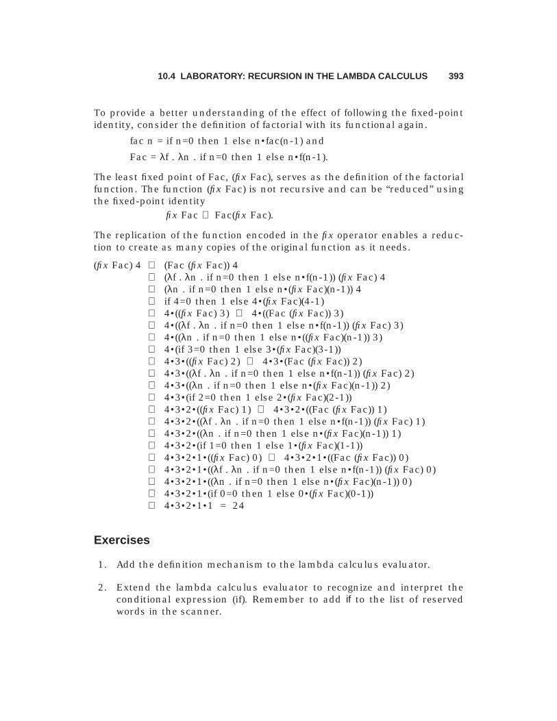
393

To provide a better understanding of the effect of following the fixed-pointidentity, consider the definition of factorial with its functional again.

fac n = if n=0 then 1 else n•fac(n-1) and

Fac = λf . λn . if n=0 then 1 else n•f(n-1).

The least fixed point of Fac, (fix Fac), serves as the definition of the factorialfunction. The function (fix Fac) is not recursive and can be “reduced” usingthe fixed-point identity

fix Fac ⇒ Fac(fix Fac).

The replication of the function encoded in the fix operator enables a reduc-tion to create as many copies of the original function as it needs.

(fix Fac) 4 ⇒ (Fac (fix Fac)) 4⇒ (λf . λn . if n=0 then 1 else n•f(n-1)) (fix Fac) 4⇒ (λn . if n=0 then 1 else n•(fix Fac)(n-1)) 4⇒ if 4=0 then 1 else 4•(fix Fac)(4-1)⇒ 4•((fix Fac) 3) ⇒ 4•((Fac (fix Fac)) 3)⇒ 4•((λf . λn . if n=0 then 1 else n•f(n-1)) (fix Fac) 3)⇒ 4•((λn . if n=0 then 1 else n•((fix Fac)(n-1)) 3)⇒ 4•(if 3=0 then 1 else 3•(fix Fac)(3-1))⇒ 4•3•((fix Fac) 2) ⇒ 4•3•(Fac (fix Fac)) 2)⇒ 4•3•((λf . λn . if n=0 then 1 else n•f(n-1)) (fix Fac) 2)⇒ 4•3•((λn . if n=0 then 1 else n•(fix Fac)(n-1)) 2)⇒ 4•3•(if 2=0 then 1 else 2•(fix Fac)(2-1))⇒ 4•3•2•((fix Fac) 1) ⇒ 4•3•2•((Fac (fix Fac)) 1)⇒ 4•3•2•((λf . λn . if n=0 then 1 else n•f(n-1)) (fix Fac) 1)⇒ 4•3•2•((λn . if n=0 then 1 else n•(fix Fac)(n-1)) 1)⇒ 4•3•2•(if 1=0 then 1 else 1•(fix Fac)(1-1))⇒ 4•3•2•1•((fix Fac) 0) ⇒ 4•3•2•1•((Fac (fix Fac)) 0)⇒ 4•3•2•1•((λf . λn . if n=0 then 1 else n•f(n-1)) (fix Fac) 0)⇒ 4•3•2•1•((λn . if n=0 then 1 else n•(fix Fac)(n-1)) 0)⇒ 4•3•2•1•(if 0=0 then 1 else 0•(fix Fac)(0-1))⇒ 4•3•2•1•1 = 24

Exercises

1. Add the definition mechanism to the lambda calculus evaluator.

2. Extend the lambda calculus evaluator to recognize and interpret theconditional expression (if). Remember to add if to the list of reservedwords in the scanner.



3. Show that each of the following expressions is a fixed-point operator inthe lambda calculus:

Yr = λh . (λg . λx . h (g g) x) (λg . λx . h (g g) x)

Yf = λh . (λx . h (λy . x x y)) (λx . h (λy . x x y))

Yg = (λx . λy . y (x x y)) (λx . λy . y (x x y))

4. Using the following definitions, calculate fib 4 by applying the Fixed-Point Identity.

G = λg . λn . if n=0 then 0 else if n=1 then 1 else g(n-1) + g(n-2)

fib = fix G = fix (λg . λn . if n<2 then n else g(n-1) + g(n-2)).

5. Add several relational operators, such as = and <, to the lambda calcu-lus evaluator and use them to test other recursive definitions.

10.5 FURTHER READING

Many of the books that contain material on denotational semantics also treatdomain theory. In particular, see [Allison86], [Schmidt88], [Stoy77], and[Watt91]. David Schmidt’s book has a chapter on recursively defined do-mains, including the inverse limit construction that justifies their existence.[Paulson87] also contains material on domain theory. For a more advancedtreatment of domain theory, see [Mosses90] and [Gunter90]. Dana Scott’sdescription of domains and models for the lambda calculus may be found in[Scott76], [Scott80], and [Scott82].

The early papers on fixed-point semantics [Manna72] and [Manna73] are agood source of examples, although the notation shows its age. Much of thismaterial is summarized in [Manna74]. This book contains a proof of the theo-rem about admissible predicates for fixed-point induction. [Bird76] also con-tains considerable material on fixed-point semantics.

Most books on functional programming or the lambda calculus contain dis-cussions of the paradoxical combinator and the fixed-point identity. Goodexamples include [Field88], [Peyton Jones87], and [Reade89]. For an advancedpresentation of recursion in the lambda calculus, see [Barendregt84].

Chapter 10 DOMAIN THEORY AND FIXED-POINT...

Documents

Transcript of Chapter 10 DOMAIN THEORY AND FIXED-POINT...