Chapter 10 Cosmic Microwave Background...

Karl-Heinz Kampert – Univ. Wuppertal Cosmology WS 2006/200796

Chapter 10

Cosmic MicrowaveBackground Radiation


Discovery of CMB

97

G. Gamow

Penzias & Wilson

Measurements in 1965 @4.08 GHz (7.35 cm)

1978


COBE Satellite (1989-1993)

98

COsmic Background Explorer FIRAS: Far Infrared Absolute Spectrophotometer

30-3000 GHz (10 - 0.1 mm)

2006


CMB Spectrum

99


High Precision 3K Measurement

100

FIRAS Instrument: T = 2.726±0.010 (Mather et al, ApJ 420 (1994) 439)

World-Data: Tγ=2.725±0.001 K


COBE Satellite (1989-1993)

101

DMR: Differential MicrowaveRadiometers7° opening angle separated by 60°

31.5, 53, and 90 GHz (9.5, 5.7, 3.3 mm)

COsmic Background Explorer


DMR @ 53 GHz

„The Eyes of God“

T = 2.728 K

Dipol-Anisotropy (v≈371 km/s)ΔT = 3.372±0.007 mKtowards Virgo Cluster(l, b) = (264.14°, 48.26°)

ΔT ≈ 18 µKAfter correction of DA (red band: Milky Way)


!"#$"%&'()*"+,$-+.

/ )*"012"(3454(6 7!

/ 8&",9(34:3(6 ;!

/ )*,&9(<(=2102"-*"(6 >!

/ ?@**+(!"#$%&#34::(6 5!

/ A-- B(;54"7(0@C-


Big Bang Singularity

Last scattering surface

Recombination

Galaxies

Here and Now

! z=1

1000

203

1500

"

Horizon1–00 8522A2

Last Scattering Surface

104

Regions of CMB sphere separated by more than ~ 1.5° cannot be causally connected


CHAPTER 3. THE EARLY UNIVERSE 70

The Horizon and Flatness Problems

• we have seen earlier that the particle horizon is given by

!w(t1, t2) =c

H0

!"0

" a(t2)

a(t1)

daa2!n/2 (3.39)

in the early universe, i.e. before curvature and cosmological-constant terms became relevant

• at recombination, the universe is well in the matter-dominatedepoch, so we can set n = 3; inserting further a(t1) = 0 and a(t2) =arec in (3.39) yields

!w(0, trec) =2cH0

!"0arec " 175

!"0 h!1 Mpc (3.40)

this is the comoving radius of a sphere around an given point inthe recombination shell which could have causal contact with thispoint before recombination

• the angular-diameter distance from us to the recombination shellis

Dang(0, zrec) "2cH0

arec

#1 ! #arec

$" 2c

H0arec " 5 h!1 Mpc (3.41)

• the angular size of the particle horizon at recombination on theCMB sky is therefore

!rec =arec!w(0, arec)

Dang(0, zrec)"!"0arec " 1.7$

!"0 (3.42)

Size of causally connected regionson the CMB

• given any point on the microwave sky, the causally connected re-gion around it has a radius of approximately one degree, i.e. fourtimes the radius of the full moon; how is it possible that theCMB temperature is so very closely the same all over the fullsky? points on the sky further apart than " 2$ had no chance ofcausally interacting and “communicating” their temperature; thisconstitutes the horizon problem

• ignoring the cosmological-constant term, the Friedmann equationcan be written

H2(a) =8"G

3# ! Kc2

a2 = H2(a)%"total(a) ! Kc2

a2H2

&(3.43)

thus the deviation of "total from unity is

|"total ! 1| = Kc2

a2H2 (3.44)


Horizon Problem

106

T1 T1 = T2

T2

Tdec = 0.3 eV

Our Hubble radius at

decoupling

T0 = 3 K

Universe expansion (z = 1100)

Our observable

universe today

Fig. 26: Perhaps the most acute problem of the Big Bang theory is explaining the extraordinary homogeneity and isotropy of the

microwave background, see Fig. 10. At the time of decoupling, the volume that gave rise to our present universe contained many

causally disconnected regions (top figure). Today we observe a blackbody spectrum of photons coming from those regions and

they appear to have the same temperature, T1 = T2, to one part in 105. Why is the universe so homogeneous? This constitutes

the so-called horizon problem, which is spectacularly solved by inflation. From Ref. [70].

energy density, which drives the exponential expansion during inflation, see Fig. 27. We know from gen-

eral relativity that the density of matter determines the expansion of the universe, but a constant energy

density acts in a very peculiar way: as a repulsive force that makes any two points in space separate at

exponentially large speeds. (This does not violate the laws of causality because there is no information

carried along in the expansion, it is simply the stretching of space-time.)

This superluminal expansion is capable of explaining the large scale homogeneity of our observ-

able universe and, in particular, why the microwave background looks so isotropic: regions separated

today by more than 1! in the sky were, in fact, in causal contact before inflation, but were stretched tocosmological distances by the expansion. Any inhomogeneities present before the tremendous expansion

would be washed out. This explains why photons from supposedly causally disconneted regions have

actually the same spectral distribution with the same temperature, see Fig. 26.

Moreover, in the usual Big Bang scenario a flat universe, one in which the gravitational attraction

of matter is exactly balanced by the cosmic expansion, is unstable under perturbations: a small deviation

from flatness is amplified and soon produces either an empty universe or a collapsed one. As we dis-

cussed above, for the universe to be nearly flat today, it must have been extremely flat at nucleosynthesis,

deviations not exceeding more than one part in 1015. This extreme fine tuning of initial conditions was

also solved by the inflationary paradigm, see Fig. 28. Thus inflation is an extremely elegant hypothesis

that explains how a region much, much greater that our own observable universe could have become

smooth and flat without recourse to ad hoc initial conditions. Furthermore, inflation dilutes away any

“unwanted” relic species that could have remained from early universe phase transitions, like monopoles,

cosmic strings, etc., which are predicted in grand unified theories and whose energy density could be so

large that the universe would have become unstable, and collapsed, long ago. These relics are diluted by


WMAP SatelliteWilkinson Microwave Anisotropy ProbeLaunch: 2002Δθ ~ 15 arc-min


Position of WMAP

108

Lagrange Points


No Big Bang

1 20 1 2 3

expands forever

!1

0

1

2

3

2

3

closed

Supernovae

CMB

Clusters

SNe: Knop et al. (2003)CMB: Spergel et al. (2003)Clusters: Allen et al. (2002)

"#

"M

open

flat

recollapses eventually

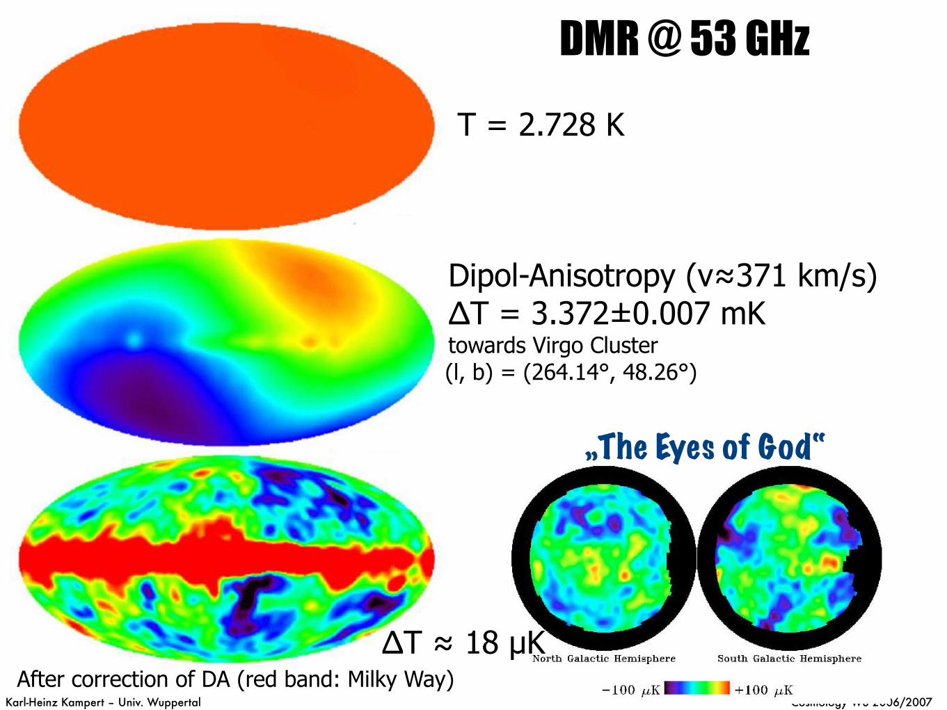
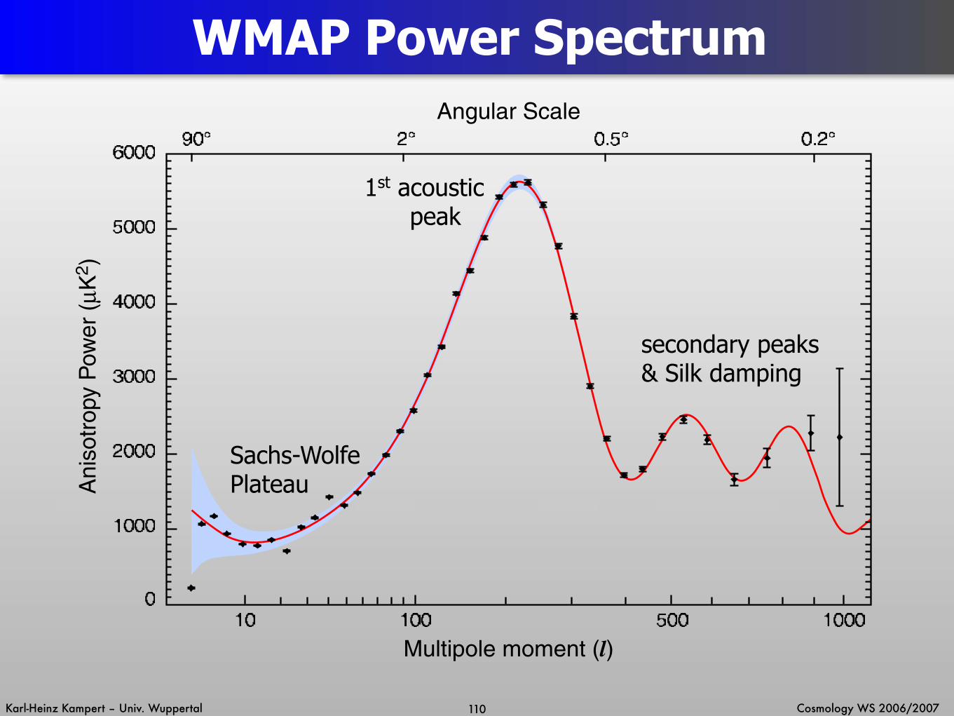
WMAP Power Spectrum

110

Sachs-WolfePlateau

1st acoustic peak

secondary peaks& Silk damping


Cosmological Parameters in CMB

111

0.2 0.4 0.6 0.8

20

40

60

80

100

T(K)

tot

0.2 0.4 0.6 0.8 1.0

bh2

100.02 0.04 0.06

100 1000

20

40

60

80

100

l

T(K)

10 100 1000

l

mh2

0.1 0.2 0.3 0.4 0.5

(a) Curvature (b) Dark Energy

(c) Baryons (d) Matter

W. Hu, S. Dodelson, Ann. Rev. Astron. Astrophys. 2002

2T= l(l+1) cl T

2

2π


No Big Bang

1 2 0 1 2 3

expands forever

-1

0

1

2

3

2

3

closed

recollapses eventually

Supernovae

CMB

Clusters

open

flat

Knop et al. (2003)Spergel et al. (2003)Allen et al. (2002)

Supernova Cosmology Project

!

!"

M

Cosmic Harmony


Planck SatelliteESALaunch: 1st quarter 2007Δθ ~ 5 arc-minsensitivity: ~10-6 K


1.4 SPACECRAFT 13

FIG 1.10.—The Planck optical system, including the telescope ba!e and V-grooves, which provide straylightcontrol in addition to thermal isolation. The attachment points for the LFI focal plane unit can be seen in the upperright. The reflectors are under manufacture by Astrium Gmbh (Friedrichshafen) together with the telescope supportstructure (under manufacture by Contraves, Zurich). Views courtesy of Alcatel Space (Cannes). The telescopefield-of-view is o"set from the spin axis of the satellite by an angle of 85!. The footprint of the field-of-view on thesky is seen in the lower left; it covers about 8! on the sky at its widest. Each spot corresponds to the 20 dB contourof the radiation pattern; the ellipticities seen are also representative of the shape of the beam at full-width-half-maximum. The black crosses indicate the orientation of the pairs of linearly polarised detectors within each horn.The field-of-view sweeps the sky in the horizontal direction in this diagram.

tube which carries the satellite loads. The propellant tanks, and the tanks containing cryogensfor the HFI coolers, are located inside the tube. Most other units are located outside the tube,mounted on side panels of the octagonal box, allowing them to radiate to space.

An attitude control system maintains the satellite rotation speed at 1 rpm, and keeps theSun direction less than 10! from the spin axis, ensuring thermal stability and full electrical powerfor the payload. A star tracker pointed along the telescope boresight measures the spin rate,the spin axis direction, and the satellite nutation. These will be used for attitude reconstructionon the ground. The reconstruction process will achieve a detector pointing accuracy of about0.!5, and will require periodic calibration using payload detections of celestial sources.

Focal Plane


Planck Position

115


Thomson Scattering: Origin of CMB Polarisation

116


Damping

• further damping occurs due to imperfect coupling between thephotons and the baryons; the photons exert a random walk andcan thus di!use across the length scale

!D =!

N! (3.24)

where ! is the mean free path of the photons

! =1

ne"T(3.25)

with the Thomson cross section "T, and the number of collisionsper unit time is

dN = ne"Tcdt (3.26)

thus,

!2D =

! trec

0

cdtne"T

(3.27)

• structures smaller than the di!usion length are damped, hencedamping sets in for wave numbers

k > kD =2#!D

(3.28)

Polarisation

• Thomson scattering is anisotropic; its di!erential cross section is

d"d"=

3"T

8#

"""$e" · $e"""2 (3.29)

where $e" and $e are the unit vectors in the directions of the in-coming and outgoing electric fields, respectively; evidently, thescattered electric field with a field vector orthogonal to that of theincoming field has zero intensity

Origin of the CMB polarisation• if the infalling radiation is isotropic, the scattered radiation is un-

polarised; if, however, the infalling radiation has a quadrupolarintensity anisotropy, the scattered radiation is polarised becauseit has di!erent intensities in its two orthogonal polarisation direc-tions

• since the electrons within the last-scattering shell are irradiated byanisotropic light, the CMB is expected to be linearly polarised tosome degree; the intensity of the polarised light should be of order10% that of the unpolarised light, i.e. it should have an amplitudeof order 10#6 K

Quadrupole inhomogeinities of matter at time of decoupling an reionisation epochs are frozen in polarization pattern

First detected by DASI Experiment at South Pole


• polarisation was first detected in the CMB by the Dasi experimentlocated at the Amundsen-Scott station at the South Pole; its am-plitude, power spectrum and and cross-power spectrum with thetemperature agree very well with expectations from theory; theWMAP satellite has measured the cross-power spectrum betweentemperature and polarisation only, which agrees very well withthe theoretical expectations derived from the temperature powerspectrum

The DASI interferometer at theAmundsen-Scott station at theSouth Pole

• the European satellite Planck will obtain full-sky maps of theCMB temperature and polarisation with an angular resolution of! 5! at frequencies between 30 and 857 GHz, further substantiallyimproving upon the results from WMAP

Temperature and polarsation mapproduced by DASI

The European Planck satelliteplanned for launch in 2007

3.1.3 Foregrounds

• originating at redshift z " 1100, the CMB shines through theentire visible universe on its way to us; it is thus hidden behind asequence of foreground layers

• the most important ones of those are caused by the microwaveemission from our own Galaxy; warm dust in the plane ofthe Milky Way with a temperature near 20 K produces emis-sion mainly above the CMB peak frequency; electrons gyrat-ing in the Galactic magnetic field emit synchrotron radiationwhich has a power law falling from radio frequencies into themicrowave regime; thermal free-free emission (bremsstrahlung)from ionised hydrogen partially falls into the microwave regime;further sources include, e.g. the line emission from molecules likeCO

• hot plasma in galaxy clusters inverse-Compton scatters mi-crowave background photons to higher energies, giving rise to theso-called Sunyaev-Zel’dovich e!ect in the microwave regime; thecharacteristic spectral behaviour of that e!ect will enable futureCMB missions to detect of order 104 galaxy clusters out to highredshifts

• other types of point source appearing in the microwave back-ground include high-redshift galaxies, and planets, asteroids, andpossibly comets in the Solar System; also, dust in the plane of theSolar System emits the so-called Zodiacal light, which adds faintmicrowave emission

• while these microwave foregrounds need to be carefully sub-tracted from the microwave sky to arrive at the CMB, they them-selves provide important data sets for cosmology, but also for re-search on the Galaxy and possibly also the Solar System


WMAP (first 3 years)

117

6 Page et al.

FIG. 3.— P and ! maps for K, Ka, and Q bands in Galactic coordinates. See Bennett et al. (2003b, Figure 4) for features and coordinates. There is only onepolarization map for K and Ka bands. For Q band, there are two maps which have been coadded. The maps are smoothed to 2!. The polarization vectors areplotted whenever a r4 HEALPix pixel (see §4.2, roughly 4deg!4deg) and three of its neighbors has a signal to noise (P/N) greater than unity. The length of thearrow is logarithmically dependent on the magnitude of P. Note that P is positive. Maps of the noise bias have been subtracted in these images.

between the A and B side beam shapes is due to the differ- ence in shapes of the primary mirrors and is self consistently

Polarisation and γ-map at 22.5 GHz.γis is the angle between the polarization direction of the electric field and the Galactic meridian.

The polarisation seen is mostly foreground due to Galactic synchrotron radiation and thermal dust emission.

Page et al. astro-ph/0603450


WMAP (first 3 years)

118

30 Page et al.

1 10 100 1000Multipole moment (l)

0.01

0.10

1.00

10.00

100.00

{ l(

l+1

) C

l /

2! }

1/2

[µ

K]

FIG. 25.— Plots of signal for TT (black), TE (red), EE (green) for the best fit model. The dashed line for TE indicates areas of anticorrelation. The cosmicvariance is shown as a light swath around each model. It is binned in ! in the same way as the data. Thus, its variations reflect transitions between ! bin sizes. Allerror bars include the signal times noise term. The ! at which each point is plotted is found from the weighted mean of the data comprising the bin. This is mostconspicuous for EE where the data are divided into bins of 2! ! ! 5, 6! ! ! 49, 50! ! ! 199, and 200 ! ! ! 799. The lowest ! point shows the cleaned QVdata, the next shows the cleaned QVW data, and the last two show the pre-cleaned QVW data. There is possibly residual foreground contamination in the secondpoint because our model is not so effective in this range as discussed in the text. For BB (blue dots), we show a model with r = 0.3. It is dotted to indicate thatat this time WMAP only limits the signal. We show the 1" limit of 0.17 µK for the weighted average of ! = 2" 10. The BB lensing signal is shown as a bluedashed line. The foreground model (Equation 25) for synchrotron plus dust emission is shown as straight dashed lines with green for EE and blue for BB. Bothare evaluated at # = 65 GHz. Recall that this is an average level and does not emphasize the !s where the emission is low.

BTT!=200 = 5589µK2. We then form:

L(! ) =1

(2")n!det(D)

exp["!

!

(#x! "#xth! )D"1(#x! "#xth! )/2]

(30)where #x! is the data as shown in Figure 21, #xth! = BEE

! (! ) is themodel !CDM spectrum,

D! =2

2$+1

1

f EEsky ($)2(BEE

! (! )+NEE! )2 (31)

as in C.14, and NEE is the uncertainty shown in Figure 21 andis derived from the MASTER spectrum determination. Weuse the symbol ! in this context because the likelihood func-tion we obtain is not the full likelihood for ! . Uncertainties

in other parameters, especially ns, have been ignored and theC! distribution is taken to be Gaussian. Thus L(! ) does notgive a good estimate of the uncertainty. Its primary use is asa simple parametrization of the data. L(! ) is plotted in Fig-ure 26 for the QV combination. We call this method “simpletau.” Table 9 shows that simple tau is stable with data selec-tion. One can also see that if the QQ component is removedfrom the QV combination, ! increases slightly. This is an-other indication that foreground emission is not biasing theresult. Additionally, one can see that removing $ = 5,7 for allband combinations does not greatly affect ! .The optimal method for computing the optical depth is with

the exact likelihood (as in Appendix D). The primary benefitsare: it makes no assumptions about the distribution of C! at

TT

TEEE

Page et al. astro-ph/0603450

Best fit cosmological modelafter correction of foregroundcontributions

BB

EE: Scalar component offluctuations (curl-free)

BB: Tensor component;predicted e.g. by inflationary scenarios(curl-free and curl)

TE: cross correlation between temp. & scalar polarisation

Chapter 10 Cosmic Microwave Background...

Documents

Transcript of Chapter 10 Cosmic Microwave Background...