Chapter 10: Contingency tables I - Department of Statistics

10.1 Introduction10.2 2× 2 contingency tables

10.4 Fishers exact test10.5 r × k contingency table

Chapter 10: Contingency tables I

Timothy Hanson

Department of Statistics, University of South Carolina

Stat 205: Elementary Statistics for the Biological and Life Sciences

1 / 25



Two-sample binary data

In Chapter 9 we looked at one sample & looked at observedvs. “expected under H0.”

Now we consider two populations and will want to comparetwo population proportions p1 and p2.

In population 1, we observed y1 out of n1 successes; inpopulation 2 we observed y2 out of n2 successes.This information can be placed in a contingency table

Group1 2

Outcome Success y1 y2

Failure n1 − y1 n2 − y2

Total n1 n2

p̂1 = y1/n1 estimates p1 & p̂2 = y2/n2 estimates p2.

2 / 25



Example 10.1.1 Migraine headache

Migraine headache patients took part in a double-blind clinicaltrial to assess experimental surgery.

75 patients were randomly assigned to real surgery onmigraine trigger sites (n1 = 49) or sham surgery (n2 = 26) inwhich an incision was made but nothing else.

The surgeons hoped that patients would experience “asubstantial reduction in migraine headaches,” which we willlabel as success.

3 / 25



Example 10.1.1 Migraine headache

p̂1 = 41/49 = 83.7% for real surgeries.

p̂2 = 15/26 = 57.7% for sham surgeries.

Real appears to be better than sham, but is this differencesignificant?

4 / 25



Example 10.1.2 HIV testing

A random sample of 120 college students found that 9 of the 61women in the sample had taken an HIV test, compared to 8 of the59 men.

p̂1 = 9/61 = 14.8% tested among women.

p̂2 = 8/59 = 13.6% tested among men.

These are pretty close.

5 / 25



Conditional probabilities

p1 and p2 are conditional probabilities. Remember way backin Section 3.3?

For the migraine data, p1 = pr{success|real} andp2 = pr{success|sham}. p̂1 = 0.84 and p̂2 = 0.58 estimatethese conditional probabilities.

For the HIV testing data, p1 = pr{tested|female} andp2 = pr{tested|male}. p̂1 = 0.15 and p̂2 = 0.14 estimatethese conditional probabilities.

6 / 25



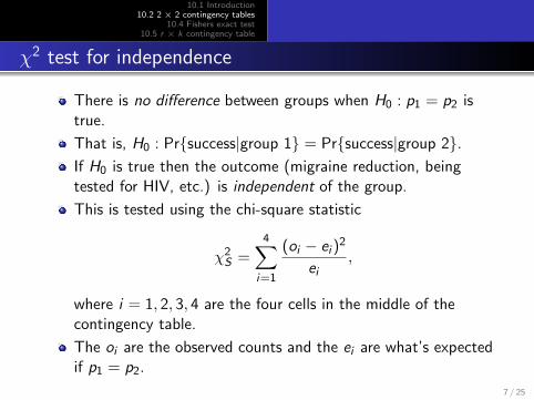
χ2 test for independence

There is no difference between groups when H0 : p1 = p2 istrue.

That is, H0 : Pr{success|group 1} = Pr{success|group 2}.If H0 is true then the outcome (migraine reduction, beingtested for HIV, etc.) is independent of the group.

This is tested using the chi-square statistic

χ2S =

4∑i=1

(oi − ei )2

ei,

where i = 1, 2, 3, 4 are the four cells in the middle of thecontingency table.

The oi are the observed counts and the ei are what’s expectedif p1 = p2.

7 / 25



Computing ei

If H0 : p1 = p2 is true then we can estimate the commonprobability p = p1 = p2 by p̂ = (y1 + y2)/(n1 + n2). This isp̂ = 56/75 = 0.747 for migraine data.

In the upper left corner we’d expect to seep̂n1 = 0.747(49) = 36.59 successes in the real surgery group,and so 49− 36.59 = 12.41 failures in the lower left.

In the upper right corner we’d expect to seep̂n2 = 0.747(26) = 19.41 successes in the sham surgerygroup, and so 26− 19.41 = 6.59 failures in the lower right.

8 / 25



Observed and expected under H0

χ2S =

(41− 36.59)2

36.59+

(15− 19.41)2

19.41+

(8− 12.41)2

12.41+

(11− 6.59)2

6.59= 6.06.

9 / 25



The P-value

When H0 : p1 = p2 is true, χ2S has a χ2

1 distribution,chi-square with 1 degree of freedom.

The P-value is the tail probability of a chi-square density with1 df greater than what we saw χ2

S . The P-value is theprobability of seeing p̂1 and p̂2 even further away from eachother than what we saw.

We can get the P-value out of R using chisq.test, but nowwe need to put in a contingency table in the form of a matrixto get our P-value.

10 / 25



Obtaining surgery data P-value in R

Need to create a 2× 2 matrix of values first> surgery=matrix(c(41,8,15,11),nrow=2)

> colnames(surgery)=c("Real","Sham")

> rownames(surgery)=c("Success","No success")

> surgery

Real Sham

Success 41 15

No success 8 11

The default chisq.test(surgery) uses

χ2Y =

∑4i=1

(|oi−ei |−0.5)2

ei. Called “Yates continuity correction”

& gives more accurate P-values in small samples.> chisq.test(surgery)

Pearson’s Chi-squared test with Yates’ continuity correction

data: surgery

X-squared = 4.7661, df = 1, p-value = 0.02902

11 / 25



Obtaining surgery data P-value in R

To get the statistic and P-value in your book, we have to turnthe Yates correction “off” usingchisq.test(surgery,correct=FALSE).> chisq.test(surgery,correct=FALSE)

Pearson’s Chi-squared test

data: surgery


We reject H0 : p1 = p2 at the 5% level. The surgerysignificantly reduces migraines.

Either P-value = 0.029 (using Yate’s) or P-value = 0.014(regular) is fine.

12 / 25



10.3 Two ways to collect data

There are two ways to collect 2× 2 contingency table data.

Cross-sectional data is collected by randomly sampling nindividuals and cross-classifying them on two variables.

Example Ask n = 143 random individuals two questions:salary high/low and education high-school/college.

The row and column totals are random.

Product binomial data is collected when a fixed numberfrom one group is sampled, and a fixed number from anothergroup is sampled.

Example: Real vs. sham surgery for migraine.

13 / 25



10.4 Fishers exact test

For the chi-square test to be valid, we cannot have very smallsample sizes, say less than 5 in any cell.

For small sample sizes there is an exact test, called Fisher’sexact test for testing H0 : p1 = p2.

Fisher’s test computes all possible 2× 2 tables with the samenumber of successes and failures (56 successes and 19 failuresfor the migraine study) that make p̂1 and p̂2 even furtherapart than what we saw, and adds up the probability of seeingeach table. Your book has details if you are interested on pp.381–383.

An alternative, that also works for small sample sizes, is theequivalent of the permutation test of Section 7.1, only forbinary data, given bychisq.test(surgery,simulate.p.value=TRUE).

14 / 25



Example 10.4.5 Flu shots

A random sample of college students found that 13 of them hadgotten a flu shot at the beginning of the winter and 28 had not.Of the 13 who had a flu shot, 3 got the flu during the winter. Ofthe 28 who did not get a flu shot, 15 got the flu.

Want to test H0 : p1 = p2 vs. H0 : p1 > p2 where p1 is probabilityof getting flu among those without shots and p2 is probability ofgetting flu among those that got shots.

15 / 25



P-value for flu shot data

Tables where p1 and p2 are even further apart in the direction ofHA : p1 > p2

P-value = 0.05298 + 0.01174 + 0.00138 + 0.00006 = 0.06616.

16 / 25



Fisher’s exact test

The probability of each table is given by the hypergeometricdistribution and is beyond the scope of this course, although yourbook does a nice job of explaining if you are interested. For the flushot data to carry out Fisher’s test we type> flu=matrix(c(15,13,3,10),nrow=2)

> fisher.test(flu,alternative="greater")

Fisher’s Exact Test for Count Data

data: flu

p-value = 0.06617

alternative hypothesis: true odds ratio is greater than 1

sample estimates:

odds ratio

3.721944

We’ll discuss what an odds ratio is next time. For now, we acceptH0 : p1 = p2 at the 5% level. There is not statistically significantevidence that getting a flu shot decreases the probability of gettingthe flu.

17 / 25



Directional alternatives

Using fisher.test we can test H0 : p1 = p2 versus one of(a) HA : p1 6= p2, (b) HA : p1 < p2, or (c) HA : p1 > p2.

Use alternative="two.sided" (the default) oralternative="less" or alternative="greater".

Fisher’s test is better than the chi-square test; just use theFisher test in your homework.

You will use chisq.test for tables larger than 2× 2 instead,our next topic...

18 / 25



10.5 r × k contingency table

The number of categories is generalized to r instead of 2.

The number of groups is generalized to k instead of 2.

Still want to test H0 : the probabilities of being in each of ther categories do not change across the k groups.

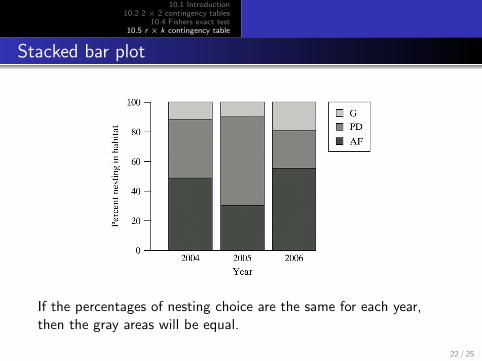
In the next example, r = 3 categories (agricultural field, prairiedog habitat, grassland) and k = 3 groups (2004, 2005, 2006).

19 / 25



Example 10.5.1 Plover Nesting

Wildlife ecologists monitored the breeding habitats of mountainplovers for three years and made note of where the plovers nested.

Question: do nesting choices vary over time?

20 / 25



Plover nesting percentages over time

21 / 25



Stacked bar plot

If the percentages of nesting choice are the same for each year,then the gray areas will be equal.

22 / 25



Chi-square test

H0 category percentages do not change across groups.

The chi-square test statistic is given by

χ2S =

∑all cells

(ei − oi )2

ei.

Here, ei is the total number in the group (column total) timesthe total row percentage, i.e.

e =row total× column total

grand total.

χ2S has a χ2

df where df = (r − 1)(k − 1). This is where theP-value comes from.

23 / 25



Plover data, observed & expected

Upper left 18.55 = 43(66)153 ,

χ2S =

(21− 18.55)2

18.55+ · · ·+ (9− 6.14)2

6.14= 14.09.

24 / 25



Chi-square test in R

> plover=matrix(c(21,17,5,19,38,6,26,12,9),nrow=3)

> plover

[,1] [,2] [,3]

[1,] 21 19 26

[2,] 17 38 12

[3,] 5 6 9

> chisq.test(plover)

Pearson’s Chi-squared test

data: plover


We reject H0 that nesting preference does not change over time atthe 5% level.

25 / 25

Chapter 10: Contingency tables I - Department of Statistics

Documents

Transcript of Chapter 10: Contingency tables I - Department of Statistics