CHAPTER 10DETERMINING HOW COSTS BEHAVE

10-1 The two assumptions are1. Variations in the level of a single activity (the cost driver) explain the variations in the

related total costs. 2. Cost behavior is approximated by a linear cost function within the relevant range. A

linear cost function is a cost function where, within the relevant range, the graph of total costs versus the level of a single activity forms a straight line.

10-2 Three alternative linear cost functions are1. Variable cost function––a cost function in which total costs change in proportion to the

changes in the level of activity in the relevant range.2. Fixed cost function––a cost function in which total costs do not change with changes in

the level of activity in the relevant range.3. Mixed cost function––a cost function that has both variable and fixed elements. Total

costs change but not in proportion to the changes in the level of activity in the relevant range.

10-3 A linear cost function is a cost function where, within the relevant range, the graph of total costs versus the level of a single activity related to that cost is a straight line. An example of a linear cost function is a cost function for use of a telephone line where the terms are a fixed charge of $10,000 per year plus a $2 per minute charge for phone use. A nonlinear cost function is a cost function where, within the relevant range, the graph of total costs versus the level of a single activity related to that cost is not a straight line. Examples include economies of scale in advertising where an agency can double the number of advertisements for less than twice the costs, step-cost functions, and learning-curve-based costs.

10-4 No. High correlation merely indicates that the two variables move together in the data examined. It is essential also to consider economic plausibility before making inferences about cause and effect. Without any economic plausibility for a relationship, it is less likely that a high level of correlation observed in one set of data will be similarly found in other sets of data.

10-5 Four approaches to estimating a cost function are1. Industrial engineering method.2. Conference method.3. Account analysis method.4. Quantitative analysis of current or past cost relationships.

10-6 The conference method estimates cost functions on the basis of analysis and opinions about costs and their drivers gathered from various departments of a company (purchasing, process engineering, manufacturing, employee relations, etc.). Advantages of the conference method include1. The speed with which cost estimates can be developed.2. The pooling of knowledge from experts across functional areas.3. The improved credibility of the cost function to all personnel.

10-1

10-7 The account analysis method estimates cost functions by classifying cost accounts in the subsidiary ledger as variable, fixed, or mixed with respect to the identified level of activity. Typically, managers use qualitative, rather than quantitative, analysis when making these cost-classification decisions.

10-8 The six steps are1. Choose the dependent variable (the variable to be predicted, which is some type of cost).2. Identify the independent variable or cost driver.3. Collect data on the dependent variable and the cost driver.4. Plot the data.5. Estimate the cost function.6. Evaluate the cost driver of the estimated cost function.Step 3 typically is the most difficult for a cost analyst.

10-9 Causality in a cost function runs from the cost driver to the dependent variable. Thus, choosing the highest observation and the lowest observation of the cost driver is appropriate in the high-low method.

10-10 Three criteria important when choosing among alternative cost functions are1. Economic plausibility.2. Goodness of fit.3. Slope of the regression line.

10-11 A learning curve is a function that measures how labor-hours per unit decline as units of production increase because workers are learning and becoming better at their jobs. Two models used to capture different forms of learning are1. Cumulative average-time learning model. The cumulative average time per unit declines

by a constant percentage each time the cumulative quantity of units produced doubles.2. Incremental unit-time learning model. The incremental time needed to produce the last

unit declines by a constant percentage each time the cumulative quantity of units produced doubles.

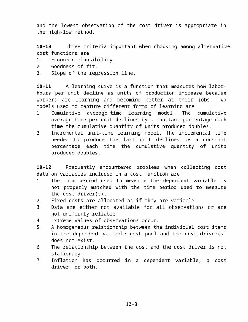
10-12 Frequently encountered problems when collecting cost data on variables included in a cost function are1. The time period used to measure the dependent variable is not properly matched with the

time period used to measure the cost driver(s).2. Fixed costs are allocated as if they are variable.3. Data are either not available for all observations or are not uniformly reliable.4. Extreme values of observations occur.5. A homogeneous relationship between the individual cost items in the dependent variable

cost pool and the cost driver(s) does not exist.6. The relationship between the cost and the cost driver is not stationary.7. Inflation has occurred in a dependent variable, a cost driver, or both.

10-2

10-13 Four key assumptions examined in specification analysis are1. Linearity of relationship between the dependent variable and the independent variable

within the relevant range.2. Constant variance of residuals for all values of the independent variable.3. Independence of residuals.4. Normal distribution of residuals.

10-14 No. A cost driver is any factor whose change causes a change in the total cost of a related cost object. A cause-and-effect relationship underlies selection of a cost driver. Some users of regression analysis include numerous independent variables in a regression model in an attempt to maximize goodness of fit, irrespective of the economic plausibility of the independent variables included. Some of the independent variables included may not be cost drivers.

10-15 No. Multicollinearity exists when two or more independent variables are highly correlated with each other.

10-16 (10 min.) Estimating a cost function.

1. Slope coefficient =

=

= = $0.35 per machine-hour

Constant = Total cost – (Slope coefficient Quantity of cost driver)

= $5,400 – ($0.35 10,000) = $1,900

= $4,000 – ($0.35 6,000) = $1,900

The cost function based on the two observations isMaintenance costs = $1,900 + $0.35 Machine-hours

2. The cost function in requirement 1 is an estimate of how costs behave within the relevant range, not at cost levels outside the relevant range. If there are no months with zero machine-hours represented in the maintenance account, data in that account cannot be used to estimate the fixed costs at the zero machine-hours level. Rather, the constant component of the cost function provides the best available starting point for a straight line that approximates how a cost behaves within the relevant range.

10-3

10-18 (20 min.) Various cost-behavior patterns.1. K2. B3. G4. J Note that A is incorrect because, although the cost per pound eventually equals a

constant at $9.20, the total dollars of cost increases linearly from that point onward.

5. I The total costs will be the same regardless of the volume level.6. L7. F This is a classic step-cost function.8. K9. C

10-20 (15 min.) Account analysis method.

1. Variable costs:Car wash labor $260,000Soap, cloth, and supplies 42,000Water 38,000Electric power to move conveyor belt 72,000

Total variable costs $412,000Fixed costs:

Depreciation $ 64,000Salaries 46,000

Total fixed costs $110,000Some costs are classified as variable because the total costs in these categories change in proportion to the number of cars washed in Lorenzo’s operation. Some costs are classified as fixed because the total costs in these categories do not vary with the number of cars washed. If the conveyor belt moves regardless of the number of cars on it, the electricity costs to power the conveyor belt would be a fixed cost.

2. Variable costs per car = = $5.15 per car

Total costs estimated for 90,000 cars = $110,000 + ($5.15 × 90,000) = $573,500

10-22(30 min.) Account analysis method.

1. Manufacturing cost classification for 2009:

Account

TotalCosts

(1)

% of Total Costs

That is Variable

(2)

VariableCosts

(3) = (1) (2)

FixedCosts

(4) = (1) – (3)

VariableCost per Unit

(5) = (3) ÷ 75,000

10-4

Direct materialsDirect manufacturing laborPowerSupervision laborMaterials-handling laborMaintenance laborDepreciationRent, property taxes, admin

$300,000225,00037,50056,25060,00075,00095,000

100,000

100%10010020504000

$300,000225,00037,50011,25030,00030,000

0 0

$ 000

45,00030,00045,00095,000

100,000

$4.003.000.500.150.400.400

0 Total $948,750 $633,750 $315,000 $8 .45

Total manufacturing cost for 2009 = $948,750

Variable costs in 2010:

Account

Unit Variable Cost per Unit for

2009(6)

Percentage Increase

(7)

Increase in Variable

Cost per Unit

(8) = (6) (7)

Variable Cost per Unit for 2010

(9) = (6) + (8)

Total Variable Costs for 2010

(10) = (9) 80,000

Direct materialsDirect manufacturing laborPowerSupervision laborMaterials-handling laborMaintenance laborDepreciationRent, property taxes, admin.

$4.003.000.500.150.400.400

0

5%10000000

$0.200.3000000

0

$4.203.300.500.150.400.400

0

$336,000264,00040,00012,00032,00032,000

0 0

Total $8 .45 $0 .50 $8 .95 $716,000

10-5

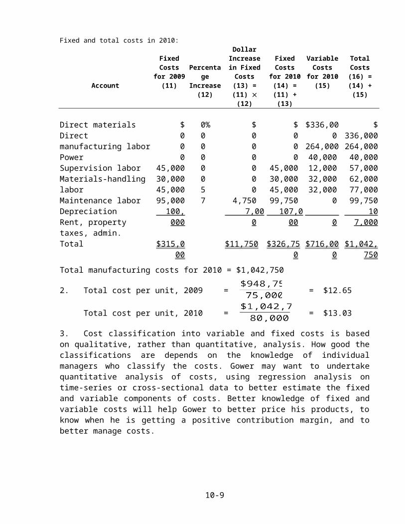
Fixed and total costs in 2010:

Account

Fixed Costs

for 2009(11)

PercentageIncrease

(12)

Dollar Increase in Fixed Costs

(13) =(11) (12)

Fixed Costsfor 2010

(14) =(11) + (13)

Variable Costs for

2010(15)

TotalCosts(16) =

(14) + (15)

Direct materialsDirect manufacturing laborPowerSupervision laborMaterials-handling laborMaintenance laborDepreciationRent, property taxes, admin.

$ 000

45,00030,00045,00095,000

100,000

0%0000057

$ 000000

4,750 7,000

$ 000

45,00030,00045,00099,750

107,000

$336,000264,00040,00012,00032,00032,000

0 0

$ 336,000264,00040,00057,00062,00077,00099,750

107,000 Total $315,000 $11,750 $326,750 $716,000 $1,042,750

Total manufacturing costs for 2010 = $1,042,750

2. Total cost per unit, 2009 = = $12.65

Total cost per unit, 2010 = = $13.03

3. Cost classification into variable and fixed costs is based on qualitative, rather than quantitative, analysis. How good the classifications are depends on the knowledge of individual managers who classify the costs. Gower may want to undertake quantitative analysis of costs, using regression analysis on time-series or cross-sectional data to better estimate the fixed and variable components of costs. Better knowledge of fixed and variable costs will help Gower to better price his products, to know when he is getting a positive contribution margin, and to better manage costs.

10-6

10-24 (20 min.) Estimating a cost function, high-low method.

1. See Solution Exhibit 10-24. There is a positive relationship between the number of service reports (a cost driver) and the customer-service department costs. This relationship is economically plausible.

2. Number of Customer-ServiceService Reports Department Costs

Highest observation of cost driver 436 $21,890Lowest observation of cost driver 122 12,941Difference 314 $ 8,949Customer-service department costs = a + b (number of service reports)

Slope coefficient (b) = = $28.50 per service report

Constant (a) = $21,890 – $28.50 436 = $9,464= $12,941 – $28.50 122 = $9,464

3. Other possible cost drivers of customer-service department costs are:a. Number of products replaced with a new product (and the dollar value of the new

products charged to the customer-service department).b. Number of products repaired and the time and cost of repairs.

SOLUTION EXHIBIT 10-24Plot of Number of Service Reports versus Customer-Service Dept. Costs for Capitol Products

10-7

$0

5,000

10,000

15,000

20,000

$25,000

0 100 200 300 400 500

Number of Service Reports

Cus

tom

er-S

ervi

ce D

epar

tmen

t Cos

ts

10-26 (20 min.) Cost-volume-profit and regression analysis.

1a. Average cost of manufacturing =

= = $30 per frame

This cost is greater than the $28.50 per frame that Ryan has quoted.

1b. Garvin cannot take the average manufacturing cost in 2009 of $30 per frame and multiply it by 36,000 bicycle frames to determine the total cost of manufacturing 36,000 bicycle frames. The reason is that some of the $900,000 (or equivalently the $30 cost per frame) are fixed costs and some are variable costs. Without distinguishing fixed from variable costs, Garvin cannot determine the cost of manufacturing 36,000 frames. For example, if all costs are fixed, the manufacturing costs of 36,000 frames will continue to be $900,000. If, however, all costs are variable, the cost of manufacturing 36,000 frames would be $30 36,000 = $1,080,000. If some costs are fixed and some are variable, the cost of manufacturing 36,000 frames will be somewhere between $900,000 and $1,080,000.

Some students could argue that another reason for not being able to determine the cost of manufacturing 36,000 bicycle frames is that not all costs are output unit-level costs. If some costs are, for example, batch-level costs, more information would be needed on the number of batches in which the 36,000 bicycle frames would be produced, in order to determine the cost of manufacturing 36,000 bicycle frames.

2. = $432,000 + $15 36,000

= $432,000 + $540,000 = $972,000

Purchasing bicycle frames from Ryan will cost $28.50 36,000 = $1,026,000. Hence, it will cost Garvin $1,026,000 $972,000 = $54,000 more to purchase the frames from Ryan rather than manufacture them in-house.

3. Garvin would need to consider several factors before being confident that the equation in requirement 2 accurately predicts the cost of manufacturing bicycle frames.

a. Is the relationship between total manufacturing costs and quantity of bicycle frames economically plausible? For example, is the quantity of bicycles made the only cost driver or are there other cost-drivers (for example batch-level costs of setups, production-orders or material handling) that affect manufacturing costs?

b. How good is the goodness of fit? That is, how well does the estimated line fit the data?

c. Is the relationship between the number of bicycle frames produced and total manufacturing costs linear?

d. Does the slope of the regression line indicate that a strong relationship exists between manufacturing costs and the number of bicycle frames produced?

e.Are there any data problems such as, for example, errors in measuring costs, trends in prices of materials, labor or overheads that might affect variable or fixed costs over

10-8

time, extreme values of observations, or a nonstationary relationship over time between total manufacturing costs and the quantity of bicycles produced?

f. How is inflation expected to affect costs?g. Will Ryan supply high-quality bicycle frames on time?

10-9

10-28 High-low, regression1. Pat will pick the highest point of activity, 3400 parts (August) at $20,500 of cost, and the lowest point of activity, 1910 parts (March) at $11560.

Cost driver:Quantity Purchased Cost

Highest observation of cost driver 3,400 $20,500Lowest observation of cost driver 1,910 11,560Difference 1,490 $ 8,940

Purchase costs = a + b Quantity purchased

Constant (a) = $20,500 ─ ($6 3,400) = $100

The equation Pat gets is:

Purchase costs = $100 + ($6 Quantity purchased)

2. Using the equation above, the expected purchase costs for each month will be:

Month

Purchase Quantity Expected Formula Expected cost

October 3,000 parts y = $100 + ($6 3,000) $18,100November 3,200 y = $100 + ($6 3,200) 19,300December 2,500 y = $100 + ($6 2,500) 15,100

3. Economic Plausibility: Clearly, the cost of purchasing a part is associated with the quantity purchased.

Goodness of Fit: As seen in Solution Exhibit 10-28, the regression line fits the data well. The vertical distance between the regression line and observations is small.

Significance of the Independent Variable: The relatively steep slope of the regression line suggests that the quantity purchased is correlated with purchasing cost for part #4599.

10-10

SOLUTION EXHIBIT 10-28

According to the regression, Pat’s original estimate of fixed cost is too low given all the data points. The original slope is too steep, but only by 16 cents. So, the variable rate is lower but the fixed cost is higher for the regression line than for the high-low cost equation.

The regression is the more accurate estimate because it uses all available data (all nine data points) while the high-low method only relies on two data points and may therefore miss some important information contained in the other data.

4. Using the regression equation, the purchase costs for each month will be:

Month

PurchaseQuantityExpected Formula Expected cost

October 3,000 parts y = $501.54 + ($5.84 3,000) $18,022November 3,200 y = $501.54 + ($5.84 3,200) 19,190December 2,500 y = $501.54 + ($5.84 2,500) 15,102

Although the two equations are different in both fixed element and variable rate, within the relevant range they give similar expected costs. In fact the estimated costs for December vary by only $2. This implies that the high and low points of the data are a reasonable representation of the total set of points within the relevant range.

10-11

10-30 (20 min.) Learning curve, incremental unit-time learning model.

1. The direct manufacturing labor-hours (DMLH) required to produce the first 2, 3, and 4 units, given the assumption of an incremental unit-time learning curve of 90%, is as follows:

90% Learning CurveCumulative

Number of Units (X)Individual Unit Time for Xth

Unit (y): Labor HoursCumulative Total Time:

Labor-Hours(1) (2) (3) 1 3,000 3,000 2 2,700 = (3,000 0.90) 5,700 3 2,539 8,239 4 2,430 = (2,700 0.90) 10,669

Values in column (2) are calculated using the formula y = aXb where a = 3,000, X = 2, 3, or 4, and b = – 0.152004, which gives

when X = 2, y = 3,000 2– 0.152004 = 2,700when X = 3, y = 3,000 3– 0.152004 = 2,539when X = 4, y = 3,000 4– 0.152004 = 2,430

Variable Costs of Producing2 Units 3 Units 4 Units

Direct materials $80,000 2; 3; 4Direct manufacturing labor $25 5,700; 8,239; 10,669Variable manufacturing overhead $15 5,700; 8,239; 10,669Total variable costs

$160,000

142,500

85,500 $388,000

$240,000

205,975

123,585 $569,560

$ 320,000

266,725

160,035 $746,760

2. Variable Costs of Producing

2 Units 4 UnitsIncremental unit-time learning model (from requirement 1)Cumulative average-time learning model (from Exercise 10-28)Difference

$388,000 376,000 $ 12,000

$746,760 708,800 $ 37,960

Total variable costs for manufacturing 2 and 4 units are lower under the cumulative average-time learning curve relative to the incremental unit-time learning curve. Direct manufacturing labor-hours required to make additional units decline more slowly in the incremental unit-time learning curve relative to the cumulative average-time learning curve when the same 90% factor is used for both curves. The reason is that, in the incremental unit-time learning curve, as the number of units double only the last unit produced has a cost of 90% of the initial cost. In the cumulative average-time learning model, doubling the number of units causes the average cost of all the additional units produced (not just the last unit) to be 90% of the initial cost.

10-12

10-32 (30min.) High-low method and regression analysis.1. See Solution Exhibit 10-32.

SOLUTION EXHIBIT 10-32Plot, High-low Line, and Regression Line for Number of Customers per Week versus Weekly Total Costs for Happy Business College Restaurant

10-13

High-low line

Regression line

2. Number of

Customers per weekWeekly

Total Costs

Highest observation of cost driver (Week 9) 925 $20,305Lowest observation of cost driver (Week 2) 745 16,597Difference 180 $ 3,708Weekly total costs = a + b (number of customers per week)

Slope coefficient (b) = = $20.60 per customer

Constant (a) = $20,305 – ($20.60 925) = $1,250= $16,597 – ($20.60 745) = $1,250

Weekly total costs = $1,250 + $20.60 (number of customers per week) See high-low line in Solution Exhibit 10-32.

3. Solution Exhibit 10-32 presents the regression line.

Economic Plausibility. The cost function shows a positive economically plausible relationship between number of customers per week and weekly total restaurant costs. Number of customers is a plausible cost driver since both cost of food served and amount of time the waiters must work (and hence their wages) increase with the number of customers served.

Goodness of fit. The regression line appears to fit the data well. The vertical differences between the actual costs and the regression line appear to be quite small.

Significance of independent variable. The regression line has a steep positive slope and increases by more than $19 for each additional customer. Because the slope is not flat, there is a strong relationship between number of customers and total restaurant costs.

The regression line is the more accurate estimate of the relationship between number of customers and total restaurant costs because it uses all available data points while the high-low method relies only on two data points and may therefore miss some information contained in the other data points. Nevertheless, the graphs of the two lines are fairly close to each other, so the cost function estimated using the high-low method appears to be a good approximation of the cost function estimated using the regression method.

4. The cost estimate by the two methods will be equal where the two lines intersect. You can find the number of customers by setting the two equations to be equal and solving for x. That is,

$1,250 + $20.60x = $2,453 + $19.04x$20.60 ─ $19.04 = $2,453 ─ $1,250

1.56 = 1,203 = 771.15 or ≈ 771customers.

10-14

10-34 (30 min.) Regression, activity-based costing, choosing cost drivers.1. Both number of units inspected and inspection labor-hours are plausible cost drivers for

inspection costs. The number of units inspected is likely related to test-kit usage, which is a significant component of inspection costs. Inspection labor-hours are a plausible cost driver if labor hours vary per unit inspected, because costs would be a function of how much time the inspectors spend on each unit. This is particularly true if the inspectors are paid a wage, and if they use electric or electronic machinery to test the units of product (cost of operating equipment increases with time spent).

2. Solution Exhibit 10-34 presents (a) the plots and regression line for number of units inspected versus inspection costs and (b) the plots and regression line for inspection labor-hours and inspection costs.

SOLUTION EXHIBIT 10-34APlot and Regression Line for Units Inspected versus Inspection Costs for Newroute Manufacturing

SOLUTION EXHIBIT 10-34BPlot and Regression Line for Inspection Labor-Hours and Inspection Costs for Newroute Manufacturing

Goodness of Fit. As you can see from the two graphs, the regression line based on number of units inspected better fits the data (has smaller vertical distances from the points to the line) than the regression line based on inspection labor-hours. The activity of inspection appears to

10-15

be more closely linearly related to the number of units inspected than inspection labor-hours. Hence number of units inspected is a better cost driver. This is probably because the number of units inspected is closely related to test-kit usage, which is a significant component of inspection costs.

Significance of independent variable. It is hard to visually compare the slopes because the graphs are not the same size, but both graphs have steep positive slopes indicating a strong relationship between number of units inspected and inspection costs, and inspection labor-hours and inspection costs. Indeed, if labor-hours per inspection do not vary much, number of units inspected and inspection labor-hours will be closely related. Overall, it is the significant cost of test-kits that is driven by the number of units inspected (not the inspection labor-hours spent on inspection) that makes units inspected the preferred cost driver.

3. At 150 inspection labor hours and 1200 units inspected,

Inspection costs using units inspected = $1,004 + ($2.02 × 1200) = $3,428

Inspection costs using inspection labor-hours = $626 + ($19.51 × 150) = $3,552.50

If Neela uses inspection-labor-hours she will estimate inspection costs to be $3,552.50, $124.50 ($3,552.50 ─$3,428) higher than if she had used number of units inspected. If actual costs equaled, say, $3,500, Neela would conclude that Newroute has performed efficiently in its inspection activity because actual inspection costs would be lower than budgeted amounts. In fact, based on the more accurate cost function, actual costs of $3,500 exceeded the budgeted amount of $3,428. Neela should find ways to improve inspection efficiency rather than mistakenly conclude that the inspection activity has been performing well.

10-16

10-36 (30–40 min.) Cost estimation, cumulative average-time learning curve.

1. Cost to produce the 2nd through the 8th troop deployment boats:

Direct materials, 7 $100,000 $ 700,000Direct manufacturing labor (DML), 39,1301 $30 1,173,900Variable manufacturing overhead, 39,130 $20 782,600Other manufacturing overhead, 25% of DML costs 293,475Total costs $2,949,975

1The direct manufacturing labor-hours to produce the second to eighth boats can be calculated in several ways, given the assumption of a cumulative average-time learning curve of 85%:

Use of table format:85% Learning Curve

Cumulative Number of Units (X)

(1)

Cumulative Average Time per Unit (y):

Labor Hours (2)

Cumulative Total Time:

Labor-Hours (3) = (1) (2)

1 10,000.00 10,0002 8,500.00 = (10,000 0.85) 17,0003 7,729.00 23,1874 7,225.00 = (8,500 0.85) 28,9005 6,856.71 34,2846 6,569.78 39,4197 6,336.56 44,3568 6,141.25 = (7,225 0.85) 49,130

The direct labor-hours required to produce the second through the eighth boats is 49,130 – 10,000 = 39,130 hours.

Use of formula: y = aXb

where a = 10,000, X = 8, and b = – 0.234465y = 10,000 8– 0.234465 = 6,141.25 hours

The total direct labor-hours for 8 units is 6,141.25 8 = 49,130 hours

The direct labor-hours required to produce the second through the eighth boats is 49,130 – 10,000 = 39,130 hours.

Note: Some students will debate the exclusion of the tooling cost. The question specifies that the tooling “cost was assigned to the first boat.” Although Nautilus may well seek to ensure its total revenue covers the $725,000 cost of the first boat, the concern in this question is only with the cost of producing seven more PT109s.

10-17

2. Cost to produce the 2nd through the 8th boats assuming linear function for direct labor- hours and units produced:

Direct materials, 7 $100,000 $ 700,000Direct manufacturing labor (DML), 7 10,000 hrs. $30 2,100,000Variable manufacturing overhead, 7 10,000 hrs. $20 1,400,000Other manufacturing overhead, 25% of DML costs 525,000Total costs $4,725,000

The difference in predicted costs is:Predicted cost in requirement 2   (based on linear cost function) $4,725,000Predicted cost in requirement 1   (based on 85% learning curve) 2,949,975Difference in favor of learning-curve based costs $1,775,025

Note that the linear cost function assumption leads to a total cost that is 60% higher than the cost predicted by the learning curve model. Learning curve effects are most prevalent in large manufacturing industries such as airplanes and boats where costs can run into the millions or hundreds of millions of dollars, resulting in very large and monetarily significant differences between the two models.

10-18

10-38 Regression; choosing among models. (chapter appendix)1. Solution Exhibit 10-38A presents the regression output for (a) setup costs and number of setups and (b) setup costs and number of setup-hours.

SOLUTION EXHIBIT 10-38ARegression Output for (a) Setup Costs and Number of Setups and (b) Setup Costs and Number of Setup-Hours

10-19

2. Solution Exhibit 10-38B presents the plots and regression lines for (a) number of setups versus setup costs and (b) number of setup hours versus setup costs.

SOLUTION EXHIBIT 10-38BPlots and Regression Lines for (a) Number of Setups versus Setup Costs and (b) Number of Setup-Hours versus Setup Costs

10-20

3. Number of Setups Number of Setup Hours

Economic plausibility

A positive relationship between setup costs and the number of setups is economically plausible.

A positive relationship between setup costs and the number of setup-hours is also economically plausible, especially since setup time is not uniform, and the longer it takes to setup, the greater the setup costs, such as costs of setup labor and setup equipment.

Goodness of fit r2 = 34%standard error of regression =$28,721Poor goodness of fit.

r2 = 85%standard error of regression =$13,558Excellent goodness of fit.

Significance of IndependentVariables

The t-value of 1.89 is not significant at the 0.05 level.

The t-value of 6.36 is significant at the 0.05 level.

Specification analysis of estimation assumptions

Based on a plot of the data, the linearity assumption holds, but the constant variance assumption may be violated. The Durbin-Watson statistic of 1.12 suggests the residuals are independent. The normality of residuals assumption appears to hold. However, inferences drawn from only 9 observations are not reliable.

Based on a plot of the data, the assumptions of linearity, constant variance, independence of residuals (Durbin-Watson = 1.50), and normality of residuals hold. However, inferences drawn from only 9 observations are not reliable.

4. The regression model using number of setup-hours should be used to estimate set up costs because number of setup-hours is a more economically plausible cost driver of setup costs (compared to number of setups). The setup time is different for different products and the longer it takes to setup, the greater the setup costs such as costs of setup-labor and setup equipment. The regression of number of setup-hours and setup costs also has a better fit, a significant independent variable, and better satisfies the assumptions of the estimation technique.

10-21

10-40 (40–50 min.) Purchasing Department cost drivers, activity-based costing, simple regression analysis.

The problem reports the exact t-values from the computer runs of the data. Because the coefficients and standard errors given in the problem are rounded to three decimal places, dividing the coefficient by the standard error may yield slightly different t-values.

1. Plots of the data used in Regressions 1 to 3 are in Solution Exhibit 10-40A. See Solution Exhibit 10-40B for a comparison of the three regression models.

2. Both Regressions 2 and 3 are well-specified regression models. The slope coefficients on their respective independent variables are significantly different from zero. These results support the Couture Fabrics’ presentation in which the number of purchase orders and the number of suppliers were reported to be drivers of purchasing department costs.

In designing an activity-based cost system, Fashion Flair should use number of purchase orders and number of suppliers as cost drivers of purchasing department costs. As the chapter appendix describes, Fashion Flair can either (a) estimate a multiple regression equation for purchasing department costs with number of purchase orders and number of suppliers as cost drivers, or (b) divide purchasing department costs into two separate cost pools, one for costs related to purchase orders and another for costs related to suppliers, and estimate a separate relationship for each cost pool.

3. Guidelines presented in the chapter could be used to gain additional evidence on cost drivers of purchasing department costs.

1. Use physical relationships or engineering relationships to establish cause-and-effect links. Lee could observe the purchasing department operations to gain insight into how costs are driven.

2. Use knowledge of operations. Lee could interview operating personnel in the purchasing department to obtain their insight on cost drivers.

10-22

SOLUTION EXHIBIT 10-40ARegression Lines of Various Cost Drivers on Purchasing Dept. Costs for Fashion Flair

Dollar Value of Merchandise Purchased(in millions)

50 100 150

500,000

1,000,000

1,500,000

2,000,000

$2,500,000

00

Number of Purchase Orders

2,000 4,000 6,000 8,000

500,000

1,000,000

1,500,000

2,000,000

$2,500,000

00

Number of Suppliers

100 200 300

500,000

1,000,000

1,500,000

2,000,000

$2,500,000

00

Purc

hasin

g D

epar

tmen

t Cos

tsPu

rcha

sing

D

epar

tmen

t Cos

tsPu

rcha

sing

D

epar

tmen

t Cos

ts

10-23

SOLUTION EXHIBIT 10-40BComparison of Alternative Cost Functions for Purchasing Department Costs Estimated with Simple Regression for Fashion Flair

CriterionRegression 1

PDC = a + (b MP$)

Regression 2PDC = a + (b # of POs)

Regression 3PDC = a + (b # of Ss)

1. Economic Plausibility

Result presented at seminar by Couture Fabrics found little support for MP$ as a driver. Purchasing personnel at the Miami store believe MP$ is not a significant cost driver.

Economically plausible. The higher the number of purchase orders, the more tasks undertaken.

Economically plausible. Increasing the number of suppliers increases the costs of certifying vendors and managing the Fashion Flair-supplier relationship.

2. Goodness of fit r2 = 0.08. Poor goodness of fit.

r2 = 0.42. Reasonable goodness of fit.

r2 = 0.39. Reasonable goodness of fit.

3. Significance of Independent Variables

t-value on MP$ of 0.84 is insignificant.

t-value on # of POs of 2.43 is significant.

t-value on # of Ss of 2.28 is significant.

4. Specification Analysis

A. Linearity within the relevant range

Appears questionable but no strong evidence against linearity.

Appears reasonable. Appears reasonable.

B. Constant variance of residuals

Appears questionable, but no strong evidence against constant variance.

Appears reasonable. Appears reasonable.

C. Independence of residuals

Durbin-WatsonStatistic = 2.41Assumption of independence is not rejected.

Durbin-WatsonStatistic = 1.98Assumption of independence is not rejected.

Durbin-WatsonStatistic = 1.97Assumption of independence is not rejected.

D. Normality of residuals

Data base too small to make reliable inferences.

Data base too small to make reliable inferences.

Data base too small to make reliable inferences.

10-24

10-42 (40 min.) High-low method, alternative regression functions, accrual accounting adjustments, ethics.

1. Solution Exhibit 10-42A presents the two data plots. The plot of engineering support reported costs and machine-hours shows two separate groups of data, each of which may be approximated by a separate cost function. The problem arises because the plant records materials and parts costs on an “as purchased” rather than an “as used” basis. The plot of engineering support restated costs and machine-hours shows a high positive correlation between the two variables (the coefficient of determination is 0.94); a single linear cost function provides a good fit to the data. Better estimates of the cost relation result because Kennedy adjusts the materials and parts costs to an accrual accounting basis.

2.Cost Driver

Machine-HoursReported Engineering

Support CostsHighest observation of cost driver (August)Lowest observation of cost driver (September)Difference

7319 54

$ 617 1,066 $ (449 )

Slope coefficient, b =

= = –$8.31 per machine-hourConstant (at highest observation of cost driver) = $ 617 – (–$8.31 73) = $1,224Constant (at lowest observation of cost driver) = $1,066 – (–$8.31 19) = $1,224The estimated cost function is y = $1,224 – $8.31X

Cost DriverMachine-Hours

Restated EngineeringSupport Costs

Highest observation of cost driver (August)Lowest observation of cost driver (September)Difference

7319 54

$966 370 $596

Slope coefficient, b =

= = $11.04 per machine-hour

Constant (at highest observation of cost driver) = $ 966 – ($11.04 73) = $160Constant (at lowest observation of cost driver) = $ 370 – ($11.04 19) = $160

The estimated cost function is y = $160 + $11.04 X

10-25

3. The cost function estimated with engineering support restated costs better approximates the regression analysis assumptions. See Solution Exhibit 10-42B for a comparison of the two regressions.

4. Of all the cost functions estimated in requirements 2 and 3, Kennedy should choose Regression 2 using engineering support restated costs as best representing the relationship between engineering support costs and machine-hours. The cost functions estimated using engineering support reported costs are mis-specified and not-economically plausible because materials and parts costs are reported on an “as-purchased” rather than on an “as-used” basis. With respect to engineering support restated costs, the high-low and regression approaches yield roughly similar estimates. The regression approach is technically superior because it determines the line that best fits all observations. In contrast, the high-low method considers only two points (observations with the highest and lowest cost drivers) when estimating the cost function. Solution Exhibit 10-42B shows that the cost function estimated using the regression approach has excellent goodness of fit (r2 = 0.94) and appears to be well specified.

5. Problems Kennedy might encounter includea. A perpetual inventory system may not be used in this case; the amounts requisitioned

likely will not permit an accurate matching of costs with the independent variable on a month-by-month basis.

b. Quality of the source records for usage by engineers may be relatively low; e.g., engineers may requisition materials and parts in batches, but not use them immediately.

c. Records may not distinguish materials and parts for maintenance from materials and parts used for repairs and breakdowns; separate cost functions may be appropriate for the two categories of materials and parts.

d. Year-end accounting adjustments to inventory may mask errors that gradually accumulate month-by-month.

6. Picking the correct cost function is important for cost prediction, cost management, and performance evaluation. For example, had United Packaging used Regression 1 (engineering support reported costs) to estimate the cost function, it would erroneously conclude that engineering support costs decrease with machine-hours. In a month with 60 machine-hours, Regression 1 would predict costs of $1,393.20 – ($14.23 60) = $539.40. If actual costs turn out to be $800, management would conclude that changes should be made to reduce costs. In fact, on the basis of the preferred Regression 2, support overhead costs are lower than the predicted amount of $176.38 + ($11.44 60) = $862.78––a performance that management should seek to replicate, not change.

On the other hand, if machine-hours worked in a month were low, say 25 hours, Regression 1 would erroneously predict support overhead costs of $1,393.20 – ($14.23 25) = $1,037.45. If actual costs are $700, management would conclude that its performance has been very good. In fact, compared to the costs predicted by the preferred Regression 2 of $176.38 + ($11.44 25) = $462.38, the actual performance is rather poor. Using Regression 1, management may feel costs are being managed very well when in fact they are much higher than what they should be and need to be managed “down.”

10-26

7. Because Kennedy is confident that the restated numbers are correct, he cannot change them just to please Mason. If he does, he is violating the standards of integrity and objectivity for management accountants. Kennedy should establish the correctness of the numbers with Mason, point out that he cannot change them, and also reason that this is a problem that could crop up each year and they should take a firm, ethical stand right away. If Mason continues to apply pressure, Kennedy has no option but to escalate the problem to higher levels in the organization. He should be prepared to resign, if necessary, rather than compromise his professional ethics.

SOLUTION EXHIBIT 10-42APlots and Regression Lines for Engineering SupportReported Costs and Engineering Support Restated Costs

10-27

0

200

400

600

800

1,000

1,200

$1,400

0 10 20 30 40 50 60 70 80

E

ngin

eeri

ng S

uppo

rt R

epor

ted

Cos

ts

Machine-Hours

200

400

600

800

1,000

$1,200

0

0 10 20 30 40 50 60 70 80

Eng

inee

ring

Sup

port

Res

tate

d C

osts

Machine-Hours

SOLUTION EXHIBIT 10-42BComparison of Alternative Cost Functions for Engineering Support Costs at United Packaging

Criterion

Regression 1Dependent Variable:Engineering Support

Reported Costs

Regression 2Dependent Variable:Engineering Support

Restated Costs1. Economic Plausibility Negative slope relationship is

economically implausible over the long run.

Positive slope relationship is economically plausible.

2. Goodness of Fit r2 = 0.43. Moderate goodness of fit.

r2 = 0.94. Excellent goodness of fit.

3. Significance of Independent Variables

t-statistic on machine-hours is statistically significant (t = –2.31), albeit economically implausible.

t-statistic on machine-hours is highly statistically significant (t=10.59).

4. Specification Analysis:A. Linearity Linearity does not describe

data very well.Linearity describes data very well.

B. Constant variance of residuals

Appears questionable, although 12 observations do not facilitate the drawing of reliable inferences.

Appears reasonable, although 12 observations do not facilitate the drawing of reliable inferences.

C. Independence of residuals

Durbin-Watson = 2.26. Residuals serially uncorrelated.

Durbin-Watson = 1.31. Some evidence of serial correlation in the residuals.

D. Normality of residuals

Database too small to make reliable inferences.

Database too small to make reliable inferences.

10-28