Chapter 1 Supplemental Text Material

S-1.1 More About Planning Experiments Coleman and Montgomery (1993) present a discussion of methodology and some guide sheets useful in the pre-experimental planning phases of designing and conducting an industrial experiment. The guide sheets are particularly appropriate for complex, high-payoff or high-consequence experiments involving (possibly) many factors or other issues that need careful consideration and (possibly) many responses. They are most likely to be useful in the earliest stages of experimentation with a process or system. Coleman and Montgomery suggest that the guide sheets work most effectively when they are filled out by a team of experimenters, including engineers and scientists with specialized process knowledge, operators and technicians, managers and (if available) individuals with specialized training and experience in designing experiments. The sheets are intended to encourage discussion and resolution of technical and logistical issues before the experiment is actually conducted.

Coleman and Montgomery give an example involving manufacturing impellers on a CNC-machine that are used in a jet turbine engine. To achieve the desired performance objectives, it is necessary to produce parts with blade profiles that closely match the engineering specifications. The objective of the experiment was to study the effect of different tool vendors and machine set-up parameters on the dimensional variability of the parts produced by the CNC-machines.

The master guide sheet is shown in Table 1 below. It contains information useful in filling out the individual sheets for a particular experiment. Writing the objective of the experiment is usually harder than it appears. Objectives should be unbiased, specific, measurable and of practical consequence. To be unbiased, the experimenters must encourage participation by knowledgeable and interested people with diverse perspectives. It is all too easy to design a very narrow experiment to “prove” a pet theory. To be specific and measurable the objectives should be detailed enough and stated so that it is clear when they have been met. To be of practical consequence, there should be something that will be done differently as a result of the experiment, such as a new set of operating conditions for the process, a new material source, or perhaps a new experiment will be conducted. All interested parties should agree that the proper objectives have been set.

The relevant background should contain information from previous experiments, if any, observational data that may have been collected routinely by process operating personnel, field quality or reliability data, knowledge based on physical laws or theories, and expert opinion. This information helps quantify what new knowledge could be gained by the present experiment and motivates discussion by all team members. Table 2 shows the beginning of the guide sheet for the CNC-machining experiment.

Response variables come to mind easily for most experimenters. When there is a choice, one should select continuous responses, because generally binary and ordinal data carry much less information and continuous responses measured on a well-defined numerical scale are typically easier to analyze. On the other hand, there are many situations where a count of defectives, a proportion, or even a subjective ranking must be used as a response.

Table 1. Master Guide Sheet. This guide can be used to help plan and design an experiment. It serves as a checklist to improve experimentation and ensures that results are not corrupted for lack of careful planning. Note that it may not be possible to answer all questions completely. If convenient, use supplementary sheets for topics 4-8

1.Experimenter's Name and Organization: Brief Title of Experiment: 2. Objectives of the experiment (should be unbiased, specific, measurable, and of practical consequence): 3. Relevant background on response and control variables: (a) theoretical relationships; (b) expert knowledge/experience; (c) previous experiments. Where does this experiment fit into the study of the process or system?: 4. List: (a) each response variable, (b) the normal response variable level at which the process runs, the distribution or range of normal operation, (c) the precision or range to which it can be measured (and how): 5. List: (a) each control variable, (b) the normal control variable level at which the process is run, and the distribution or range of normal operation, (c) the precision (s) or range to which it can be set (for the experiment, not ordinary plant operations) and the precision to which it can be measured, (d) the proposed control variable settings, and (e) the predicted effect (at least qualitative) that the settings will have on each response variable: 6. List: (a) each factor to be "held constant" in the experiment, (b) its desired level and allowable s or range of variation, (c) the precision or range to which it can measured (and how), (d) how it can be controlled, and (e) its expected impact, if any, on each of the responses: 7. List: (a) each nuisance factor (perhaps time-varying), (b) measurement precision, (c)strategy (e.g., blocking, randomization, or selection), and (d) anticipated effect: 8. List and label known or suspected interactions: 9. List restrictions on the experiment, e.g., ease of changing control variables, methods of data acquisition, materials, duration, number of runs, type of experimental unit (need for a split-plot design), “illegal” or irrelevant experimental regions, limits to randomization, run order, cost of changing a control variable setting, etc.: 10. Give current design preferences, if any, and reasons for preference, including blocking and randomization: 11. If possible, propose analysis and presentation techniques, e.g., plots, ANOVA, regression, plots, t tests, etc.: 12. Who will be responsible for the coordination of the experiment? 13. Should trial runs be conducted? Why / why not?

Table 2. Beginning of Guide Sheet for CNC-Machining Study.

l.Experimenter's Name and Organization: John Smith, Process Eng. Group Brief Title of Experiment: CNC Machining Study 2. Objectives of the experiment (should be unbiased, specific, measurable, and of practical consequence): For machined titanium forgings, quantify the effects of tool vendor; shifts in a-axis, x- axis, y-axis, and z-axis; spindle speed; fixture height; feed rate; and spindle position on the average and variability in blade profile for class X impellers, such as shown in Figure 1. 3. Relevant background on response and control variables: (a) theoretical relationships; (b) expert knowledge/experience; (c) previous experiments. Where does this experiment fit into the study of the process or system? (a) Because of tool geometry, x-axis shifts would be expected to produce thinner blades, an undesirable

characteristic of the airfoil. (b) This family of parts has been produced for over 10 years; historical experience indicates that

externally reground tools do not perform as well as those from the “internal” vendor (our own regrind operation).

(c) Smith (1987) observed in an internal process engineering study that current spindle speeds and feed rates work well in producing parts that are at the nominal profile required by the engineering drawings - but no study was done of the sensitivity to variations in set-up parameters.

Results of this experiment will be used to determine machine set-up parameters for impeller machining. A robust process is desirable; that is, on-target and low variability performance regardless of which tool vendor is used. Measurement precision is an important aspect of selecting the response variables in an experiment. Insuring that the measurement process is in a state of statistical control is highly desirable. That is, ideally there is a well-established system of insuring both accuracy and precision of the measurement methods to be used. The amount of error in measurement imparted by the gauges used should be understood. If the gauge error is large relative to the change in the response variable that is important to detect, then the experimenter will want to know this before conducting the experiment. Sometimes repeat measurements can be made on each experimental unit or test specimen to reduce the impact of measurement error. For example, when measuring the number average molecular weight of a polymer with a gel permeation chromatograph (GPC) each sample can be tested several times and the average of those molecular weight reading reported as the observation for that sample. When measurement precision is unacceptable, a measurement systems capability study may be performed to attempt to improve the system. These studies are often fairly complicated designed experiments. Chapter 13 presents an example of a factorial experiment used to study the capability of a measurement system. The impeller involved in this experiment is shown in Figure 1. Table 3 lists the information about the response variables. Notice that there are three response variables of interest here.

Figure 1. Jet engine impeller (side view). The z-axis is vertical, x-axis is horizontal, y-axis is into the page. 1 = height of wheel, 2 = diameter of wheel, 3 = inducer blade height, 4 = exducer blade height, 5 = z height of blade.

Table 3. Response Variables Response variable

(units) Normal operating level and range

Measurement precision, accuracy

how known?

Relationship of response variable to

objective Blade profile

(inches) Nominal (target) ±1 X 10-3 inches to ±2 X 10-3 inches at

all points

σE≈@ 1 X 10 -5 inches from a coordinate

measurement machine capability

study

Estimate mean absolute difference from target and standard deviation

Surface finish Smooth to rough

(requiring hand finish)

Visual criterion (compare to standards)

Should be as smooth as possible

Surface defect

count Typically 0 to 10 Visual criterion

(compare to standards)

Must not be excessive in number or magnitude

As with response variables, most experimenters can easily generate a list of candidate design factors to be studied in the experiment. Coleman and Montgomery call these control variables. We often call them controllable variables, design factors, or process variables in the text. Control variables can be continuous or categorical (discrete). The ability of the experimenters to measure and set these factors is important. Generally,

small errors in the ability to set, hold or measure the levels of control variables are of relatively little consequence. Sometimes when the measurement or setting error is large, a numerical control variable such as temperature will have to be treated as a categorical control variable (low or high temperature). Alternatively, there are errors-in-variables statistical models that can be employed, although their use is beyond the scope of this book. Information about the control variables for the CNC-machining example is shown in Table 4. Table 4. Control Variables Measurement Precision and Proposed settings, Predicted effects Control variable Normal level setting error- based on (for various (units) and range how known? predicted effects responses) x-axis shift* 0-.020 inches .001inches 0, .015 inches Difference (inches) (experience) y-axis shift* 0-.020 inches .001inches 0, .015 inches Difference (inches) (experience) z-axis shift* 0-.020 inches .001inches ? Difference (inches) (experience) Tool vendor Internal, external - Internal, external External is more variable a-axis shift* 0-.030 degrees .001 degrees 0, .030 degrees Unknown (degrees) (guess) Spindle speed 85-115% ∼1% 90%,110% None? (% of (indicator nominal) on control panel) Fixture height 0-.025 inches .002inches 0, .015 inches Unknown (guess) Feed rate (% of 90-110% ∼1% 90%,110% None? nominal) (indicator on control panel) 'The x, y, and z axes are used to refer to the part and the CNC machine. The a axis refers only to the machine. Held-constant factors are control variables whose effects are not of interest in this experiment. The worksheets can force meaningful discussion about which factors are adequately controlled, and if any potentially important factors (for purposes of the present experiment) have inadvertently been held constant when they should have been included as control variables. Sometimes subject-matter experts will elect to hold too many factors constant and as a result fail to identify useful new information. Often this information is in the form of interactions among process variables. In the CNC experiment, this worksheet helped the experimenters recognize that the machine had to be fully warmed up before cutting any blade forgings. The actual procedure used was to mount the forged blanks on the machine and run a 30-minute cycle

without the cutting tool engaged. This allowed all machine parts and the lubricant to reach normal, steady-state operating temperature. The use of a typical (i.e., mid-level) operator and the use of one lot of forgings ware decisions made for experimental “insurance”. Table 5 shows the held-constant factors for the CNC-machining experiment.

Table 5. Held-Constant Factors Desired experi- Measurement Factor mental level and precision-how How to control Anticipated (units) allowable range known? (in experiment) effects Type of cutting Standard type Not sure, but Use one type None fluid thought to be adequate Temperature of 100- 100°F. when 1-2° F. (estimate) Do runs after None cutting fluid machine is machine has (degrees F.) warmed up reached 100° Operator Several operators - Use one "mid- None normally work level" in the process operator Titanium Material Precision of lab Use one lot Slight forgings properties may tests unknown (or block on vary from unit forging lot, to unit only if necessary) Nuisance factors are variables that probably have some effect on the response, but which are of little or no interest to the experimenter. They differ from held-constant factors in that they either cannot be held entirely constant, or they cannot be controlled at all. For example, if two lots of forgings were required to run the experiment, then the potential lot-to-lot differences in the material would be a nuisance variable than could not be held entirely constant. In a chemical process we often cannot control the viscosity (say) of the incoming material feed stream—it may vary almost continuously over time. In these cases, nuisance variables must be considered in either the design or the analysis of the experiment. If a nuisance variable can be controlled, then we can use a design technique called blocking to eliminate its effect. Blocking is discussed initially in Chapter 4. If the nuisance variable cannot be controlled but it can be measured, then we can reduce its effect by an analysis technique called the analysis of covariance, discussed in Chapter 14. Table 6 shows the nuisance variables identified in the CNC-machining experiment. In this experiment, the only nuisance factor thought to have potentially serious effects was the machine spindle. The machine has four spindles, and ultimately a decision was made to run the experiment in four blocks. The other factors were held constant at levels below which problems might be encountered.

Table 6. Nuisance Factors Measurement Strategy (e.g., Nuisance factor precision-how randomization, (units) known? blocking, etc.) Anticipated effects Viscosity of Standard viscosity Measure viscosity at None to slight cutting fluid start and end Ambient 1-2° F. by room Make runs below Slight, unless very temperature (°F.) thermometer 80'F. hot weather (estimate) Spindle Block or randomize Spindle-to-spindle on machine spindle variation could be large Vibration of ? Do not move heavy Severe vibration can machine during objects in CNC introduce variation operation machine shop within an impeller Coleman and Montgomery also found it useful to introduce an interaction sheet. The concept of interactions among process variables is not an intuitive one, even to well-trained engineers and scientists. Now it is clearly unrealistic to think that the experimenters can identify all of the important interactions at the outset of the planning process. In most situations, the experimenters really don’t know which main effects are likely to be important, so asking them to make decisions about interactions is impractical. However, sometimes the statistically-trained team members can use this as an opportunity to teach others about the interaction phenomena. When more is known about the process, it might be possible to use the worksheet to motivate questions such as “are there certain interactions that must be estimated?” Table 7 shows the results of this exercise for the CNC-machining example.

Table 7. Interactions

Control variable

y shift

z shift

Vendor

a shift

Speed

Height

Feed

x shift P y shift - P z shift - - P Vendor - - - P a shift - - - - Speed - - - - - F,D Height - - - - - - NOTE: Response variables are P = profile difference, F = surface finish and D = surface defects Two final points: First, an experimenter without a coordinator will probably fail. Furthermore, if something can go wrong, it probably will, so he coordinator will actually have a significant responsibility on checking to ensure that the experiment is being conducted as planned. Second, concerning trial runs, this is often a very good idea—particularly if this is the first in a series of experiments, or if the experiment has high

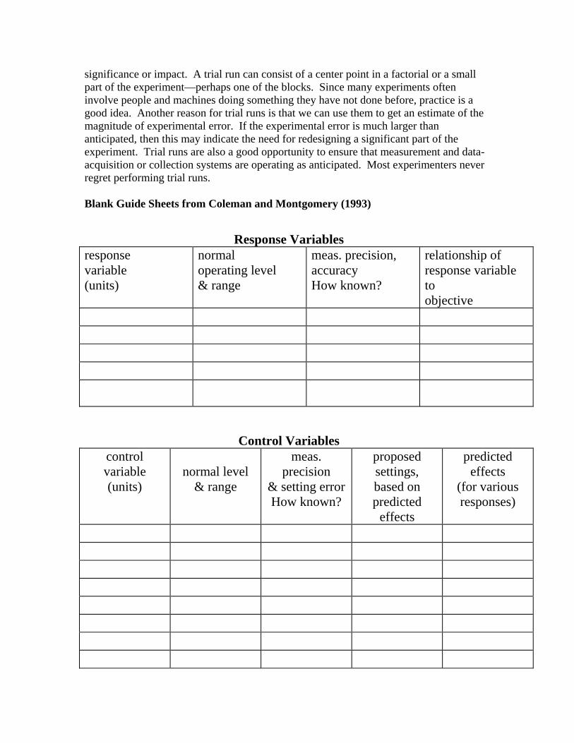
significance or impact. A trial run can consist of a center point in a factorial or a small part of the experiment—perhaps one of the blocks. Since many experiments often involve people and machines doing something they have not done before, practice is a good idea. Another reason for trial runs is that we can use them to get an estimate of the magnitude of experimental error. If the experimental error is much larger than anticipated, then this may indicate the need for redesigning a significant part of the experiment. Trial runs are also a good opportunity to ensure that measurement and data-acquisition or collection systems are operating as anticipated. Most experimenters never regret performing trial runs. Blank Guide Sheets from Coleman and Montgomery (1993)

Response Variables

response variable (units)

normal operating level & range

meas. precision, accuracy How known?

relationship of response variable to objective

Control Variables control variable (units)

normal level

& range

meas. precision

& setting error How known?

proposed settings, based on predicted

effects

predicted effects

(for various responses)

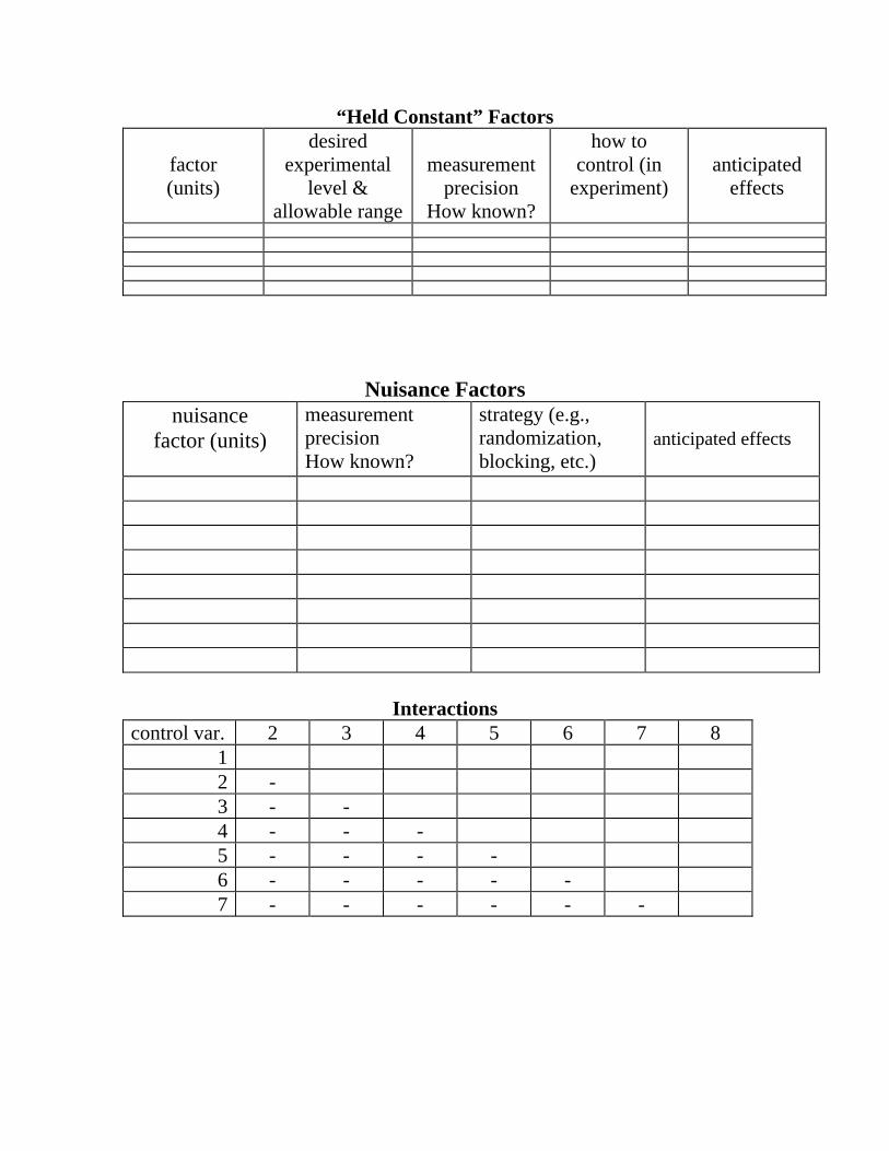
“Held Constant” Factors

factor (units)

desired experimental

level & allowable range

measurement

precision How known?

how to control (in

experiment)

anticipated

effects

Nuisance Factors nuisance

factor (units)

measurement precision How known?

strategy (e.g., randomization, blocking, etc.)

anticipated effects

Interactions control var. 2 3 4 5 6 7 8

1 2 - 3 - - 4 - - - 5 - - - - 6 - - - - - 7 - - - - - -

S-1.2 Other Graphical Aids for Planning Experiments In addition to the tables in Coleman and Montgomery’s Technometrics paper, there are a number of useful graphical aids to pre-experimental planing. Perhaps the first person to suggest graphical methods for planning an experiment was Andrews (1964), who proposed a schematic diagram of the system much like Figure 1-1 in the textbook, with inputs, experimental variables, and responses all clearly labeled. These diagrams can be very helpful in focusing attention on the broad aspects of the problem.

Barton (1997) (1998) (1999) has discussed a number of useful graphical aids in planning experiments. He suggests using IDEF0 diagrams to identify and classify variables. IDEF0 stands for Integrated Computer Aided Manufacturing Identification Language, Level 0. The U. S. Air Force developed it to represent the subroutines and functions of complex computer software systems. The IDEF0 diagram is a block diagram that resembles Figure 1-1 in the textbook. IDEF0 diagrams are hierarchical; that is, the process or system can be decomposed into a series of process steps or systems and represented as a sequence of lower-level boxes drawn within the main block diagram.

Figure 2 shows an IDEF0 diagram [from Barton (1999)] for a portion of a videodisk manufacturing process. This figure presents the details of the disk pressing activities. The primary process has been decomposed into five steps, and the primary output response of interest is the warp in the disk.

The cause-and-effect diagram (or fishbone) discussed in the textbook can also be useful in identifying and classifying variables in an experimental design problem. Figure 3 [from Barton (1999)] shows a cause-and-effect diagram for the videodisk process. These diagrams are very useful in organizing and conducting “brainstorming” or other problem-solving meetings in which process variables and their potential role in the experiment are discussed and decided.

Both of these techniques can be very helpful in uncovering intermediate variables. These are variables that are often confused with the directly adjustable process variables. For example, the burning rate of a rocket propellant may be affected by the presence of voids in the propellant material. However, the voids are the result of mixing techniques, curing temperature and other process variables and so the voids themselves cannot be directly controlled by the experimenter.

Some other useful papers on planning experiments include Bishop, Petersen and Trayser (1982), Hahn (1977) (1984), and Hunter (1977).

Figure 2. An IDEF0 Diagram for an Experiment in a Videodisk Manufacturing Process

Figure 2. A Cause-and-Effect Diagram for an Experiment in a Videodisk Manufacturing Process

S-1.3 Montgomery’s Theorems on Designed Experiments Statistics courses, even very practical ones like design of experiments, tend to be a little dull and dry. Even for engineers, who are accustomed to taking much more exciting courses on topics such as fluid mechanics, mechanical vibrations, and device physics. Consequently, I try to inject a little humor into the course whenever possible. For example, I tell them on the first class meeting that they shouldn’t look so unhappy. If they had one more day to live they should choose to spend it in a statistics class—that way it would seem twice as long.

I also use the following “theorems” at various times throughout the course. Most of them relate to non-statistical aspects of DOX, but they point out important issues and concerns. Theorem 1. If something can go wrong in conducting an experiment, it will. Theorem 2. The probability of successfully completing an experiment is inversely proportional to the number of runs. Theorem 3. Never let one person design and conduct an experiment alone, particularly if that person is a subject-matter expert in the field of study. Theorem 4. All experiments are designed experiments; some of them are designed well, and some of them are designed really badly. The badly designed ones often tell you nothing. Theorem 5. About 80 percent of your success in conducting a designed experiment results directly from how well you do the pre-experimental planning (steps 1-3 in the 7-step procedure in the textbook). Theorem 6. It is impossible to overestimate the logistical complexities associated with running an experiment in a “complex” setting, such as a factory or plant. Finally, my friend Stu Hunter has for many years said that without good experimental design, we often end up doing PARC analysis. This is an acronym for

Planning After the Research is Complete

What does PARC spell backwards?

Supplemental References Andrews, H. P. (1964). “The Role of Statistics in Setting Food Specifications”, Proceedings of the Sixteenth Annual Conference of the Research Council of the American Meat Institute, pp. 43-56. Reprinted in Experiments in Industry: Design, Analysis, and Interpretation of Results, eds. R. D. Snee, L. B. Hare and J. R. Trout, American Society for Quality Control, Milwaukee, WI 1985.

Barton, R. R. (1997). “Pre-experiment Planning for Designed Experiments: Graphical Methods”, Journal of Quality Technology, Vol. 29, pp. 307-316.

Barton, R. R. (1998). “Design-plots for Factorial and Fractional Factorial Designs”, Journal of Quality Technology, Vol. 30, pp. 40-54.

Barton, R. R. (1999). Graphical Methods for the Design of Experiments, Springer Lecture Notes in Statistics 143, Springer-Verlag, New York.

Bishop, T., Petersen, B. and Trayser, D. (1982). “Another Look at the Statistician’s Role in Experimental Planning and Design”, The American Statistician, Vol. 36, pp. 387-389.

Hahn, G. J. (1977). “Some Things Engineers Should Know About Experimental Design”, Journal of Quality Technology, Vol. 9, pp. 13-20.

Hahn, G. J. (1984). “Experimental Design in a Complex World”, Technometrics, Vol. 26, pp. 19-31.

Hunter, W. G. (1977). “Some Ideas About Teaching Design of Experiments With 25 Examples of Experiments Conducted by Students”, The American Statistician, Vol. 31, pp. 12-17.