CHAPTER 1ON THE REGULARITY OF THE GLOBAL ATTRACTOR OF A

WEAKLY DAMPED, FORCED KORTEWEG-DEVRIES EQUATION

1. Introduction

We are interested in the long time behavior of the solutions of the Korteweg-deVries

equation with a weak dissipation and an external forcing term. The Korteweg-

deVries equation (without dissipation or forcing term) was initially derived by D.

J. Korteweg and G. deVries [10] as a model for one directional long water waves

of small amplitude, and it was later shown to model a number of other physical

systems related to the propagation of one-directional waves in nonlinear, dispersive

media when the nonlinearity and dispersion have comparable effects, the dispersion

relation has a particular form, and the nonlinearity is weak and quadratic (e.g.

magnetosonic waves and ion-sound waves). In many real situations, however, one

cannot neglect energy dissipation mechanisms and external excitation, especially for

the long-time behavior. Several energy dissipation mechanisms were derived by E.

Ott and R. N. Sudan [15] depending on the physical situation. We consider here a

weak dissipation which has no smoothing effect.

More precisely, we consider the following nonlinear evolution equation for an un-

known scalar function u = u(x, t), x, t ∈ R:

ut + uux + uxxx + γu = f, (1.1)

7

with the external force f = f(x) and the dissipation coefficient γ, γ > 0, given. We

supplement this equation with the space-periodicity boundary condition

u(x+ L, t) = u(x, L), ∀x, t ∈ R. (1.2)

with L > 0 given.

Under the assumption that f ∈ H2per(0, L), the problem (1.1)-(1.2) was studied by

J. M. Ghidaglia [5, 6] as a dynamical system in H2per(0, L), and the existence of the

global attractor was obtained. Our aim in this work is to study the regularity of the

global attractor when the forcing term is more regular.

We assume f ∈ Hkper(0, L), k ∈ N, k ≥ 3 and we show that for each m = 3, . . . , k,

(1.1) and (1.2) define a dynamical system in Hmper(0, L) possessing a global attractor

Am. It is easy to see that Ak ⊂ . . . ⊂ A3, and a natural (regularity) question

is whether they are all equal. The answer is in general positive for parabolic-type

equations due to the regularization of the solutions. The answer is also positive

for some wave-type equations when there is a regularization of the solutions of the

linear part of the equation with respect to the nonhomogeneous term, in which case

the result is obtained through a splitting of the equation into two equations, one

absorbing the initial condition and the other with the nonlinear term as a forcing

term (see J. M. Ghidaglia and R. Temam [7]).

For the problem (1.1)-(1.2), however, there is no suitable regularization with re-

spect to either the initial condition or the forcing term, so that the argument used in

the previous cases do not apply directly and the result is not obvious. It turns out

thought that we can construct a different splitting of the equation which enables us

to deduce that, indeed, the attractors are equal and, hence, that the attractor is as

regular as the forcing term. This is our main result.

8

The splitting is obtained by writing the solution u of (1.1)-(1.2) with u(0) = u0 as

u = v + z where v solvesvt +Q(vvx) + vxxx + γv = f − P (uux),

v(0) = Pu0,

(1.3)

and z solves zt +Q((vz)x + zzx) + zxxx + γz = 0,

z(0) = Qu0,

(1.4)

and where P = PN is the orthogonal projection onto the first N Fourier components,

N ∈ N large enough, and Q = I − P .

We can then show that v is as regular as the forcing term while z decays ex-

ponentially to zero in an appropriate norm. Then, we can deduce that A3 is in-

cluded and bounded in Hkper(0, L), which implies that A3 = Ak, and hence that

A3 = A4 = . . . = Ak. Note, however, that since there is no regularization, if

u0 ∈ Hmper(0, L), 3 ≤ m ≤ k, then the solution u(t) is attracted to Ak ⊂ Hk

per(0, L)

in the topology of Hmper(0, L).

We should mention here that due to the lack of regularity we were not able to

show that the attractor in H2per(0, L) obtained by J. M. Ghidaglia [5, 6] is also more

regular and equal to A3, . . . ,Ak. We should also mention that in a recent work,

O. Goubet [8] considered the same regularity problem for the attractor of a weakly

damped nonlinear Schrodinger equation using a similar decomposition.

The article is organized as follows. In Section 2 we describe the equation and its

mathematical setting and state some preliminary results which will be used in the

sequel. Section 3 contains the proof of the existence of the attractors A3, . . . ,Ak.

In Section 4 the splitting described above is introduced and the regularity of the

9

attractors is obtained. The Appendix contains a sketch of the proofs of the results

stated in Section 2.

2. Preliminaries

In this section we describe the equation and its mathematical setting and state

some general results concerning the existence and uniqueness of solutions, the con-

tinuous dependence on the initial conditions, and the energy equations verified by

the solutions. The proofs of these results will be sketched in Section 5.

We consider the following nonlinear evolution equation for an unknown scalar

function u = u(x, t), x ∈ R, t ∈ R:

∂u

∂t+ u

∂u

∂x+∂3u

∂x3+ γu = f, (2.1)

where f and γ are given, with γ > 0 in the case of interest to us. We supplement

this equation with the space-periodicity boundary condition

u(x+ L, t) = u(x, t), ∀x ∈ R,∀t ∈ R, (2.2)

with L > 0 given, and with the initial condition

u(x, 0) = u0(x), ∀x ∈ R. (2.3)

For the functional setting of the problem we consider the Sobolev spaces Hkper(Ω)

of periodic functions, where k is a nonnegative integer and Ω = (0, L), endowed with

the following norm:

‖u‖k =

(k∑j=0

L2j|u|2j

)1/2

, (2.4)

where

|u|j =

(∫Ω

|Dju|2 dx)1/2

, D =∂

∂x. (2.5)

10

The space H0per(Ω) is simply L2(Ω), and for k ≥ 1, functions in Hk

per(Ω) are bounded

continuous functions on [0, L]. Indeed, it is easy to deduce the following explicit

form of the Agmon inequality:

‖u‖∞ = sup0≤x≤L

|u(x)| ≤ |u|1/20 (2|u|1 + L−1|u|0)1/2, ∀u ∈ Hkper(Ω), (2.6)

for k ≥ 1. In case the function has zero average, we have simply

‖u‖∞ ≤√

2|u|1/20 |u|1/21 , ∀u ∈ Hk

per(Ω),

∫Ω

u(x) dx = 0,

for k ≥ 1. We also write (·, ·)L2 for the usual inner-product in L2(Ω).

We assume u0, f ∈ Hkper(Ω), k ≥ 2 and study the problem (2.1), (2.2), (2.3) as

a dynamical system in Hkper(Ω). The existence and uniqueness of solutions for this

problem in H2per(Ω) for the case γ = 0 and f = 0 was proved by R. Temam [18] and

later by J. L. Bona and R. Smith [4] with the help of three polynomial invariants.

In the case γ and f are not zero, these polynomials are no longer invariant, but

satisfy some energy-like equations and are important (see Section 3) for the study of

the long time behavior of the solutions, as well as for the proof of the existence of

solutions. The original Korteweg-deVries(KdV) equation (equation(2.1) with γ = 0

and f = 0) possesses in fact an infinite number of polynomial invariants, which

follow in particular from its exact integrability via Inverse Scattering Theory (see,

e.g., [13], [11], [14]). The polynomial invariants are of the form

Im(u) =

∫Ω

[(Dmu)2 − αmu(Dm−1u)2 +Qm(u,Du, . . . , Dm−2u)] dx, m = 0, 1, 2, . . . ,

(2.7)

where D = ∂/∂x and Qm = Qm(u,Du, · · · , Dm−2u) is a polynomial composed only

of monomials of rank m + 2, where the rank of a monomial ua0(Du)a1 . . . (Dlu)al

(aj ≥ 0 integer, j = 0, 1, . . . , l) is defined as∑l

j=0(1 + j/2)aj. For m = 0, 1, we

11

simply set Qm ≡ 0 in formula (2.7). Because of the rapid proliferation of terms

with increasing rank, it is very difficult to find more explicit recursive formulas for

expressing these invariants Im(u).

We write Qm = Qm(u,Du, · · · , Dm−2u) as a linear combination of all possible

terms of rank m+2, but consider only the irreducible terms, i.e., the terms which do

not have the highest-derivative factor occurring linearly. This one for the following

reason: if a term is not irreducible, then it can be integrated by parts and expressed

as a combination of irreducible terms. The coefficients of Qm, as well as αm, can be

obtained through the method of undetermined coefficients [11], which is as follows:

We consider

d

dtIm(u) =

d

dt

∫Ω

[(Dmu)2 − αmu(Dm−1u)2 +Qm(u,Du, . . . , Dm−2u)

]dx

=

∫Ω

[2DmuDmut − αmut(Dm−1u)2 − 2αmuD

m−1uDm−1ut

+m−2∑j=0

∂Qm

∂yj(u,Du, . . . , Dm−2u)Djut

]dx

=

∫Ω

[2(−1)mD2mu− αm(Dm−1u)2 + 2αm(−1)mDm−1(uDm−1u)

+m−2∑j=0

(−1)jDj(∂Qm

∂yj(u,Du, . . . , Dm−2u))

]ut dx,

and denote

Lm(u) =2(−1)mD2mu− αm(Dm−1u)2 + 2αm(−1)mDm−1(uDm−1u)

+m−2∑j=0

(−1)jDj(∂Qm

∂yj(u,Du, . . . , Dm−2u)).

(2.8)

Then, we have

d

dtIm(u) =

∫Ω

Lm(u)ut dx. (2.9)

12

In order for Im(u) to be invariant for the KdV equation, we must impose

(Lm(u), uDu+D3u

)L2 = 0. (2.10)

After making several integrations by parts in order to obtain only irreducible terms

in (2.10), we demand that this final expression vanishes identically. Thus we find αm

and the polynomial Qm.

In case f and γ do not vanish, we obtain instead the following energy equation:

d

dtIm(u) + γ(u, Lm(u))L2 = (f, Lm(u))L2 .

Using (2.7) and (2.8), we obtain after integration by parts

d

dtIm(u) + 2γIm(u) = Km(u), (2.11)

where

Km(u) =

∫Ω

[2DmfDmu− αmf(Dm−1u)2 − 2αmuD

m−1uDm−1f

+ γαmu(Dm−1u)2 + 2γQm(u,Du, . . . , Dm−2u)

+m−2∑j=0

(Djf − γDju)∂Qm

∂yj(u,Du, . . . , Dm−2u)

]dx.

(2.12)

With the help of the energy equations (2.11) we have the following result (see also

[5]):

Theorem 2.1. For γ ∈ R, f ∈ Hkper(Ω) and u0 ∈ Hk

per(Ω), k ≥ 2, there exists a

unique solution u of (2.1)-(2.3) satisfying

u ∈ L∞(0, T ;Hkper(Ω)) ∩ C([0, T ], L2(Ω)), ∀T > 0. (2.13)

Note that replacing simultaneously x and t by −x and −t results in the same equa-

tion (2.1) with γ and f replaced by −γ and −f , respectively. Therefore, Theorem 2.1

says that the solutions exist for all t ∈ R. Then, we have

13

Theorem 2.2. Let γ ∈ R and f ∈ Hkper(Ω), k ≥ 2. Then, for every u0 ∈ Hk

per(Ω),

the solution u = u(t) of (2.1)-(2.3) restricted to [−T, T ] belongs to C([−T, T ], Hkper(Ω)),

for all T > 0. Hence, we can define on Hkper(Ω) the group S(k)(t)t∈R given by

S(k)(t)u0 = u(t), ∀t ∈ R, (2.14)

for all u0 ∈ Hkper(Ω), where u(t) is the solution of (2.1)-(2.3) at time t. For each

t ∈ R, S(k)(t) is weakly and strongly continuous on Hkper(Ω); moreover, the following

estimate holds:

sup|t|≤T‖u0‖k≤R

∥∥S(k)(t)u0

∥∥k≤ C(R, T ), ∀T,R > 0, (2.15)

where C(R, T ) is a constant depending on R and T , as well as on L, γ and ‖f‖k.

As a corollary of the proof of Theorem 2.2, we have the following result:

Corollary 2.3. For γ ∈ R, f ∈ Hkper(Ω) and u0 ∈ Hk

per(Ω), k ≥ 2, the solution

u(t) = S(k)(t)u0, t ∈ R, satisfies the energy equations (2.11) for m = 0, 1, . . . , k.

One way to prove Theorem 2.1 and Theorem 2.2 is to use the energy equation

(2.11) with m = 0, 1, . . . , k. However, a simpler way is to use (2.11) with m = 0, 1, 2

to prove the result for k = 2 and then to use some commutator estimates as done by

[17] for the original KdV equation to obtain the result for k > 2. These estimates

will also be useful for our study of the regularity of the global attractor and for this

reason we state them below.

Lemma 2.4. Let u, v belong to Hkper(Ω), k ∈ N, and let β ∈ R, β > 1/2. Then,

|Dk(uv)− uDkv|0 ≤ c(β, k, L) ‖u‖k‖v‖β + ‖u‖1+β‖v‖k−1 , (2.16)

14

where the norm ‖ · ‖s for a noninteger s ∈ R can be defined by

‖u‖2s = L

∑j∈Z

(1 + (2π)2|j|2

)s |uj|2, for u =∑j∈Z

uje2πijx/L,

which is equivalent to the norm defined previously when s in a nonnegative integer.

The proof follows easily from the Leibniz rule, the continuous imbedding ofHβper(Ω)

into L∞(Ω) for β > 1/2, and interpolation inequalities. The result is also true when

k is real (see [17]), k > 1, in which case Dk is replaced by the k/2 fractional power

of the positive operator −D2.

3. Existence of the global attractor

In this section we assume γ > 0 and consider f ∈ Hkper(Ω) given, with k ≥ 2 fixed.

First, we show in the following proposition that there exists a bounded absorbing

set in Hkper(Ω) for S(k)(t)t∈R.

Proposition 3.1. There exists a constant ρk = ρk(γ, L, ‖f‖k) such that for every

R > 0 there exists Tk = Tk(R, γ, L, ‖f‖k) such that

‖S(k)(t)u0‖k ≤ ρk, ∀t ≥ Tk,∀u0 ∈ Hkper(Ω), ‖u0‖k ≤ R.

Proof. The case k = 2 was done by J. M. Ghidaglia [5], but we include it here for

completeness. The proof is obtained using the energy equations (2.11) for m =

0, 1, . . . , k. We first need some intermediate results:

Step I. Time-uniform a priori estimates in L2(Ω) and H1per(Ω).

For m = 0, we have L0(u) = 2u, and thus the energy equation (2.11)m=0 becomes

d

dt|u|20 + 2γ|u|20 = 2

∫Ω

fu dx. (3.1)

15

Therefore,

d

dt|u|20 + 2γ|u|20 ≤ 2|f |0|u|0 ≤ γ|u|20 +

1

γ|f |20,

which gives

|u(t)|20 ≤ |u0|20e−γt +|f |20γ2

, ∀t ≥ 0. (3.2)

Consequently,

|u(t)|0 ≤2|f |0γ

, ∀t ≥ T0, (3.3)

where

T0 = T0(|u0|0, γ, |f |0) =1

γlog

(γ2|u0|203|f |20

).

For m = 1, a simple computation using the method of undetermined coefficients

described in Section 2 yields (see [5])

I1(u) =

∫Ω

[(Du)2 − 1

3u3

]dx (α1 =

1

3), (3.4)

and

L1(u) = −2D2u− u2. (3.5)

Hence, the energy equation (2.11) for m = 1 becomes

d

dtI1(u) + 2γI1(u) =

γ

3

∫Ω

u3 dx+

∫Ω

[2DfDu− fu2

]dx. (3.6)

We estimate∣∣∣∣∫Ω

u3 dx

∣∣∣∣ ≤|u|20‖u‖∞ ≤ (using the Agmon inequality (2.6))

≤|u|5/20

(2|u|1 +

1

L|u|0)1/2

≤√

2|u|5/20 |u|1/21 + L−1/2|u|30

≤(by the Young inequality) ≤ |u|21 +3

4|u|10/3

0 + L−1/2|u|30.

(3.7)

16

From (3.4) and (3.7) we deduce that

|u|21 ≤3

2I1(u) +

3

8|u|10/3

0 +1

2L1/2|u|30, (3.8)

and also

I1(u) ≤ 4

3|u|21 +

1

4|u|10/3

0 +1

3L1/2|u|30. (3.9)

We then estimate (3.6) as follows:

d

dtI1(u) + 2γI1(u) ≤γ

3

[|u|21 +

3

4|u|10/3

0 +1

L1/2|u|30]

+ 2|f |1|u|1 + ‖f‖∞|u|20

≤2γ

3|u|21 +

γ

4|u|10/3

0 +γ

3L1/2|u|30 +

3

γ|f |21 + ‖f‖∞|u|20

≤(using (3.8))

≤γI1(u) +γ

2|u|10/3

0 +2γ

3L1/2|u|30 +

3

γ|f |21 + ‖f‖∞|u|20.

Therefore,

d

dtI1(u) + γI1(u) ≤ γ

2|u|10/3

0 +2γ

3L1/2|u|30 +

3

γ|f |21 + ‖f‖∞|u|20. (3.10)

Using now (3.2) and (3.10), we find that

d

dtI1(u) + γI1(u) ≤cγ

[|u0|10/3

0 e−53γt +

|f |10/30

γ10/3

]

+cγ

L1/2

[|u0|30e−

32γt +

|f |30γ3

]+

3

γ|f |21 + ‖f‖∞

[|u0|20e−γt +

|f |20γ2

], ∀t ≥ 0,

(3.11)

for a numerical constant c > 0.

We deduce from (3.11) that

d

dtI1(u) + γI1(u) ≤ c1e

− γ2t + c2, ∀t ≥ 0, (3.12)

17

where

c1 = c[γ|u0|10/3

0 + γL−1/2|u0|30 + ‖f‖∞|u0|20]

and

c2 = c[γ−7/3|f |10/3

0 + γ−2L−1/2|f |30 + γ−1|f |21 + γ−2‖f‖∞|f |20].

Then, by the Gronwall Lemma we obtain

I1(u(t)) ≤ I1(u0)e−γt +2c1

γe−

γ2t +

c2

γ, ∀t ≥ 0. (3.13)

Using (3.8), (3.9) and (3.2) in (3.13), we deduce that

|u(t)|21 ≤3

2I1(u(t)) +

3

8|u(t)|10/3

0 +1

2L1/2|u(t)|30

≤3

2I1(u0)e−γt +

3c1

γe−

γ2t +

3c2

2γ+ c

[|u0|10/3

0 e−53γt +

|f |10/30

γ10/3

]

+ cL−1/2

[|u0|30e−

32γt +

|f |30γ3

]≤3

2

[4

3|u0|21 +

1

4|u0|10/3

0 +1

3L1/2|u0|30

]e−γt +

3c1

γe−

γ2t +

3c2

2γ

+ c

[|u0|10/3

0 e−53γt +

|f |10/30

γ10/3

]+ cL−1/2

[|u0|30e−

32γt +

|f |30γ3

], ∀t ≥ 0,

where, as before, c is a numerical constant. Hence,

|u(t)|21 ≤ X1e− γ

2t + X1, ∀t ≥ 0, (3.14)

where

X1 =2|u0|21 + c|u0|10/30 + cL−1/2|u0|30 +

3c1

γ

≤c(|u0|21 + |u0|10/3

0 + L−1/2|u0|30 + γ−1‖f‖∞|u0|20) (3.15)

18

and

X1 =3c2

γ+ cγ−10/3|f |10/3

0 + cL−1/2γ−3|f |30

≤c[γ−2|f |21 + γ−3‖f‖∞|f |20 + γ−10/3|f |10/3

0 + γ−3L−1/2|f |30],

(3.16)

and c in (3.15), (3.16) is a numerical constant.

We finally deduce from (3.14) that

|u(t)|1 ≤ ρ1 = ρ1(γ, L, |f |0, |f |1, ‖f‖∞), ∀t ≥ T1, (3.17)

where T1 = T1(γ, L, |f |0, |f |1, ‖f‖∞, |u0|0, |u0|1).

Step II. Absorbing sets in Hmper(Ω) for m = 2, 3, . . . , k.

We establish their existence by an inductive argument. Let m be fixed with

2 ≤ m ≤ k. Assume that for each j = 0, 1, . . . ,m−1 there exist Mj = Mj(γ, L, ‖f‖j)

and Tj = Tj(γ, L, ‖f‖j, R) such that

|u(t)|j ≤Mj, ∀t ≥ Tj, ∀u0 ∈ Hjper(Ω), ‖u0‖j ≤ R. (3.18)

We want to show that the same statement holds for j = m. Then, we will be able

to deduce that it holds up to m = k, which proves in particular the existence of an

absorbing ball in Hkper(Ω) for S(k)(t)t∈R.

In what follows, we denote by c a generic constant which may depend on γ, L and

f , but is independent of u0.

Consider the energy equation (2.11)m, i.e.,

d

dtIm(u) + 2γIm(u) = Km(u), (3.19)

where Im(u) and Km(u) are given by (2.7) and (2.12), respectively.

19

Using the Agmon inequality and the induction hypothesis (3.18), we deduce that

‖u(t)‖∞ ≤|u(t)|1/20 (2|u(t)|1 + L−1|u(t)|0)1/2

≤M1/20 (2M1 + L−1M0)1/2, ∀t ≥ maxT0, T1,

(3.20)

and also, since Dju has zero average for j ≥ 1,

‖Dju(t)‖∞ ≤c|u(t)|1/2j |u(t)|1/2j+1

≤cM1/2j M

1/2j+1, ∀t ≥ maxTj, Tj+1, j = 1, 2, . . . ,m− 2.

(3.21)

We then have the following estimate:∣∣∣∣∫Ω

(−αm(Dm−1u)2 +Qm(u,Du, . . . , Dm−2u)

)dx

∣∣∣∣≤ c|u|2m−1 + L‖Qm(u,Du, . . . , Dm−2u)‖∞

≤ (using (3.18), (3.20) and (3.21))

≤ c, ∀t ≥ maxT0, T1, . . . , Tm−1 = T ′.

(3.22)

Therefore, we deduce from (2.7) that

|u(t)|2m − c ≤ Im(u(t)) ≤ |u(t)|2m + c, ∀t ≥ T ′. (3.23)

Now, from (2.12), we find that

Km(u) ≤2|f |m|u|m + c‖f‖∞|u|2m−1 + c‖u‖∞|u|m−1|f |m−1

+ c‖u‖∞|u|2m−1 + cL‖Qm(u,Du, . . . , Dm−2u)‖∞

+m−2∑j=0

(|f |j + γ|u|j)L∥∥∥∥∂Qm

∂yj(u,Du, . . . , Dm−2u)

∥∥∥∥∞

≤(using again (3.18), (3.20) and (3.21))

≤γ|u|2m +1

γ|f |2m + c, ∀t ≥ T ′.

(3.24)

20

From (3.19), (3.23), and (3.24) we obtain

d

dtIm(u) + γIm(u) ≤ 1

γ|f |2m + c, ∀t ≥ T ′.

Hence, by the Gronwall Lemma it follows that

Im(u(t)) ≤ Im(u(T ′))e−γ(t−T ′) +1

γ|f |2m + c, ∀t ≥ T ′, (3.25)

which together with (3.23) gives

|u(t)|2m ≤ |u(T ′)|2me−γ(t−T ′) +1

γ|f |2m + c, ∀t ≥ T ′. (3.26)

By Theorem 2.2 we know that there exists c1 = c(R, T ′) such that

‖u(t)‖m ≤ c1, ∀u0 ∈ Hmper(Ω), ‖u0‖m ≤ R, ∀t ∈ [−T ′, T ′]. (3.27)

From (3.26) and (3.27) we then obtain

|u(t)|2m ≤ c1e−γ(t−T ′) +

1

γ|f |2m + c, ∀t ≥ T ′. (3.28)

Recall that c depends only on M0,M1, . . . ,Mm−1.

Define now

M2m = 2

(1

γ|f |2m + c

)and

Tm =1

γlog

1

c1

(1

γ|f |2m + c

)+ maxT0, T1, . . . , Tm−1,

and note that Mm = Mm(γ, L, ‖f‖m) and Tm = Tm(γ, L, ‖f‖m, R). We then have

from (3.28) that

|u(t)|m ≤Mm, ∀t ≥ Tm. (3.29)

21

Remark 3.1. A more careful computation using the particular structure of the

polynomials Qm leads to the following time-uniform a priory estimates: For each

j = 0, 1, . . . , k there exist two constants

κj = κj(γ, L, |f |0, |f |1, . . . .|f |j−1, |u0|0, |u0|1, . . . , |u0|j)

and

κj = κj(γ, L, |f |0, |f |1, . . . .|f |j)

such that

|u(t)|2j ≤ κje− γ

2jt + κj, ∀t ≥ 0,

which gives a more precise expression for the time necessary for the orbits to reach

the absorbing set.

We are now in position to prove the following theorem, which is the main result

of this section.

Theorem 3.2. The semigroup S(k)(t)t≥0 possesses a global attractor Ak in Hkper(Ω),

i.e., a set Ak compact in Hkper(Ω), invariant for S(k)(t)t≥0 and which attracts all

bounded subsets of Hkper(Ω) in the sense of the semidistance in Hk

per(Ω). Moreover,

Ak is also connected in Hkper(Ω).

In order to prove Theorem 3.2, we apply the following general result given by X.

Wang in [21]:

Theorem 3.3. Let X be a uniformly convex, separable Banach space. Let S(t)t≥0

be a continuous semigroup on X which possesses a bounded absorbing set B in X

and such that, for each fixed t, S(t) is also continuous in the weak topology on X.

22

Moreover, assume that there exist two weakly continuous functionals J and K on X

and two positive constants p, γ such that

d

dt(‖S(t)u0‖p + J(S(t)u0)) + γ (‖S(t)u0‖p + J(S(t)u0)) = K(S(t)u0), ∀u0 ∈ X.

(3.30)

Then S(t) possesses a global attractor A in X:

i. A is compact in X;

ii. S(t)A = A ∀t ≥ 0;

iii. A is connected in X; and

iv. A attracts the bounded sets in X.

For the proof, see [21].

The global attractor A is the ω-limit set of the absorbing set B, i.e.,

A = ∩t≥0∪s≥tS(s)B, (3.31)

where the closure is taken in the strong topology of X.

In our case, we consider X = Hkper(Ω), which is obviously uniformly convex and

separable; we endow it temporarily with the equivalent norm

‖u‖ =(|u|20 + |u|2k

)1/2.

Add the energy equations (2.11) for m = 0 and m = k to find

d

dt

(‖S(k)(t)u0‖2 + Jk(S

(k)(t)u0))

+ 2γ(‖S(k)(t)u0‖2 + Jk(S

(k)(t)u0))

= Kk(S(k)(t)u0), ∀u0 ∈ Hk

per(Ω),

(3.32)

where

Jk(S(k)(t)u0) = Jk(u(t)) =

∫Ω

[−αku(Dk−1u)2 +Qk(u,Du, . . . , D

k−2u)]dx,

(3.33)

23

and

Kk(S(k)(t)u0) =Kk(u(t)) = Kk(u(t)) +K0(u(t))

=

∫Ω

[2DkfDku− αkf(Dk−1u)2 + 2αkuD

k−1uDk−1f

+ γαku(Dk−1u)2 + 2γQk(u,Du, . . . , Dk−2u) + 2fu

+k−2∑j=0

(Djf − γDju)∂Qk

∂yj(u,Du, . . . , Dk−2u)

]dx.

(3.34)

Note that Jk and Kk are weakly continuous on Hkper(Ω) since the imbedding of

Hkper(Ω) into Hk−1

per (Ω) is compact. The existence of an absorbing ball in Hkper(Ω) was

proved in Proposition 3.1. Hence, we can apply Theorem 3.3 to conclude that there

exists a global attractor Ak in Hkper(Ω), which completes the proof of Theorem 3.2.

Remark 3.2. The idea of using energy equations to prove the existence of the global

attractor is due to J.M. Ball [3] and was later used by J.M. Ghidaglia [6] and X.

Wang [21]. In essence, it amounts to proving the so-called asymptotic compactness

property of the semigroup (see F. Abergel [1, 2]), O. Ladyzhenskaya [12], and R.

Rosa [16]).

4. Regularity of the attractor

Let f ∈ Hkper(Ω), k ≥ 2, and γ > 0 be given. For each j = 2, 3, . . . , k we can

consider the group S(j)(t)t∈R on Hjper(Ω) defined by

S(j)(t) : Hjper(Ω)→ Hj

per(Ω), S(j)(t)u0 = u(t) for t ∈ R,

where u(t) is the solution of (2.1)-(2.3) at time t. Clearly S(j)(t)|Hj+1per (Ω) = S(j+1)(t)

for j = 2, 3, . . . , k−1. By Theorem 3.2, there exists a global attractor Aj in Hjper(Ω)

for the group S(j)(t)t∈R. Obviously A2 ⊃ A3 ⊃ · · · ⊃ Ak. Since S(j)(t)t∈R is a

group, there is no smoothing effect. Thus, a natural, nontrivial question is whether

24

these attractors are equal. We will prove below that if k ≥ 4, then A3 = A4 = · · · =

Ak. The idea of the proof is to decompose S(3)(t) as S(3)1 (t) + S

(3)2 (t), where S

(3)1 (t)

and S(3)2 (t) are not necessarily semigroups, such that S

(3)1 (t)u0 is more regular than

the solution S(3)(t)u0 (more exactly as regular as f) and ‖S(3)2 (t)u0‖1 tends to zero

as t goes to infinity, uniformly for u0 bounded in H3per(Ω).

Set

v =∑l∈Z

vle2πilx/L.

For N ∈ N, N ≥ 1, consider

PNv =∑|l|≤N

vle2πilx/L

and

QNv = v − PNv =∑|l|>N

vle2πilx/L.

PN and QN are orthogonal projectors in any Hs, s ≥ 0.

From Lemma 5.1 (with ε−p = N) we have the following estimates:

‖PNv‖m+l ≤ clNl‖PNv‖m, ∀l > 0, (4.1)

‖QNv‖m−l ≤ clN−l‖QNv‖m, for l = 0, 1, . . . ,m, (4.2)

and also

|QNv|m−l ≤ clN−l|QNv|m, for l = 0, 1, . . . ,m. (4.3)

Consider now u0 ∈ H3per(Ω), u(t) = S(3)(t)u0 and set

y(t) = PNu(t). (4.4)

25

We split the high frequency part of u, QNu, as

QNu = q + z,

where q and z verify the following problems:dq

dt+D3q + γq +QN(qDq) +QND(yq) = QNf −QN(yDy),

q(0) = 0,

(4.5)

and dz

dt+D3z + γz +QN(zDz) +QND(vz) = 0,

z(0) = QNu0,

(4.6)

where v = y + q.

We now prove the following proposition:

Proposition 4.1. Given N ≥ 1 and u0 ∈ H3per(Ω), there exist a unique solution q

of (4.5) and a unique solution z of (4.6) satisfying

q, z ∈ L∞(0, T ;QNH3per(Ω)) ∩ C([0, T ], QNL

2(Ω)), ∀T > 0. (4.7)

Moreover, there exist N ∈ N large enough and a constant c > 0, which depend on

γ, L and f , such that the following estimates hold:

|q(t)|k ≤ cNk−2, ∀t ≥ 0, (4.8)

and

|z(t)|1 ≤ ce−γ2t, ∀t ≥ 0, (4.9)

uniformly for u0 in B3, the absorbing ball in H3per(Ω) for S(3)(t)t∈R.

26

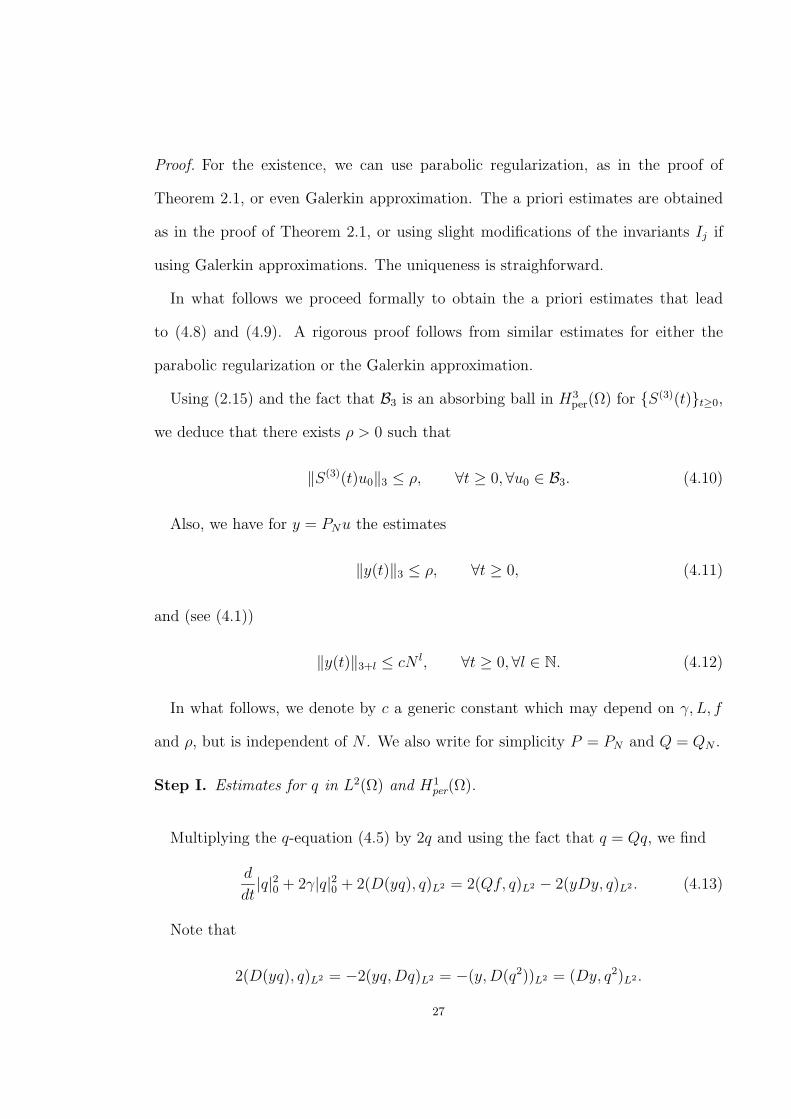
Proof. For the existence, we can use parabolic regularization, as in the proof of

Theorem 2.1, or even Galerkin approximation. The a priori estimates are obtained

as in the proof of Theorem 2.1, or using slight modifications of the invariants Ij if

using Galerkin approximations. The uniqueness is straighforward.

In what follows we proceed formally to obtain the a priori estimates that lead

to (4.8) and (4.9). A rigorous proof follows from similar estimates for either the

parabolic regularization or the Galerkin approximation.

Using (2.15) and the fact that B3 is an absorbing ball in H3per(Ω) for S(3)(t)t≥0,

we deduce that there exists ρ > 0 such that

‖S(3)(t)u0‖3 ≤ ρ, ∀t ≥ 0,∀u0 ∈ B3. (4.10)

Also, we have for y = PNu the estimates

‖y(t)‖3 ≤ ρ, ∀t ≥ 0, (4.11)

and (see (4.1))

‖y(t)‖3+l ≤ cN l, ∀t ≥ 0,∀l ∈ N. (4.12)

In what follows, we denote by c a generic constant which may depend on γ, L, f

and ρ, but is independent of N . We also write for simplicity P = PN and Q = QN .

Step I. Estimates for q in L2(Ω) and H1per(Ω).

Multiplying the q-equation (4.5) by 2q and using the fact that q = Qq, we find

d

dt|q|20 + 2γ|q|20 + 2(D(yq), q)L2 = 2(Qf, q)L2 − 2(yDy, q)L2 . (4.13)

Note that

2(D(yq), q)L2 = −2(yq,Dq)L2 = −(y,D(q2))L2 = (Dy, q2)L2 .

27

Thus, we estimate

2(Qf − yDy −D(yq), q)L2 ≤2|Qf |0|q|0 + 2‖y‖∞|y|1|q|0 + ‖Dy‖∞|q|20

≤γ|q|20 +2

γ|Qf |20 +

2

γ‖y‖2

∞|y|21 + c‖y‖2|q|20.

Hence, we deduce from (4.13) that

d

dt|q|20 + γ|q|20 ≤

2

γ|Qf |20 +

c

γρ4 + cρ|q|20.

Then,

d

dt|q|20 + γ|q|20 ≤ c1 + c2|q|20, (4.14)

where c1 = (2/γ)|Qf |20 + cρ4/γ and c2 = cρ.

Therefore, since q(0) = 0, we obtain

|q(t)|20 ≤c1

c2

ec2t, ∀t ≥ 0. (4.15)

By replacing c2 by maxc2, γ if necessary, we can assume c2 ≥ γ.

Multiply now the q-equation (4.5) by −2D2q −Q(q2)− 2Q(yq). We observe that

(D3q +Q(qDq) +QD(yq),−2D2q −Q(q2)− 2Q(yq)

)L2 = 0.

Also,

(qt,−2D2q −Q(q2)− 2Q(yq))L2 =(qt,−2D2q − q2 − 2yq)L2

=

∫Ω

(∂t(Dq)

2 − ∂t(q3

3)− y∂t(q2)

)dx

=d

dt

∫Ω

((Dq)2 − q3

3− yq2

)dx+ (yt, q

2)L2 ,

28

and

γ(q,−2D2q −Q(q2)− 2Q(yq))L2 =γ(q,−2D2q − q2 − 2yq)L2

=2γ

∫Ω

((Dq)2 − q3

2− yq2

)dx.

Therefore, we obtain

d

dt

∫Ω

((Dq)2 − q3

3− yq2

)dx+ 2γ

∫Ω

((Dq)2 − q3

2− yq2

)dx+ (yt, q

2)L2

=(Qf −Q(yDy),−2D2q −Q(q2)− 2Q(yq)

)L2 .

(4.16)

We estimate now

(Qf −Q(yDy),− 2D2q −Q(q2)− 2Q(yq))L2

=2(QDf,Dq)L2 − (Qf, q2)− 2(Qf, yq)L2 − 2(D(yDy), Dq)L2

+ (Q(yDy), q2)L2 + 2(Q(yDy), yq)L2

≤2|Qf |1|q|1 + ‖Qf‖∞|q|20 + 2|yQf |0|q|0 + |y2|2|q|1

+1

2‖QD(y2)‖∞|q|20 + |y2|1‖y‖∞|q|0

≤(2|Qf |1 + |y2|2)|q|1 + (‖Qf‖∞ +1

2‖QD(y2)‖∞)|q|20

+ (2|yQf |0 + |y2|1‖y‖∞)|q|0

≤(2|Qf |1 + c‖y‖22)|q|1 + (c‖Qf‖1 + c‖y‖2

2)|q|20

+ (2‖y‖∞|Qf |0 + c‖y‖31)|q|0

≤(using (4.11))

≤c|q|0 + c|q|20 + c|q|1.

From (4.3) we have

|q|0 ≤ c0N−1|q|1. (4.17)

29

Therefore,

(Qf −Q(yDy),−2D2q −Q(q2)− 2Q(yq)

)L2 ≤cN−1|q|1 + cN−2|q|21 + c|q|1

≤c|q|1 + cN−2|q|21.

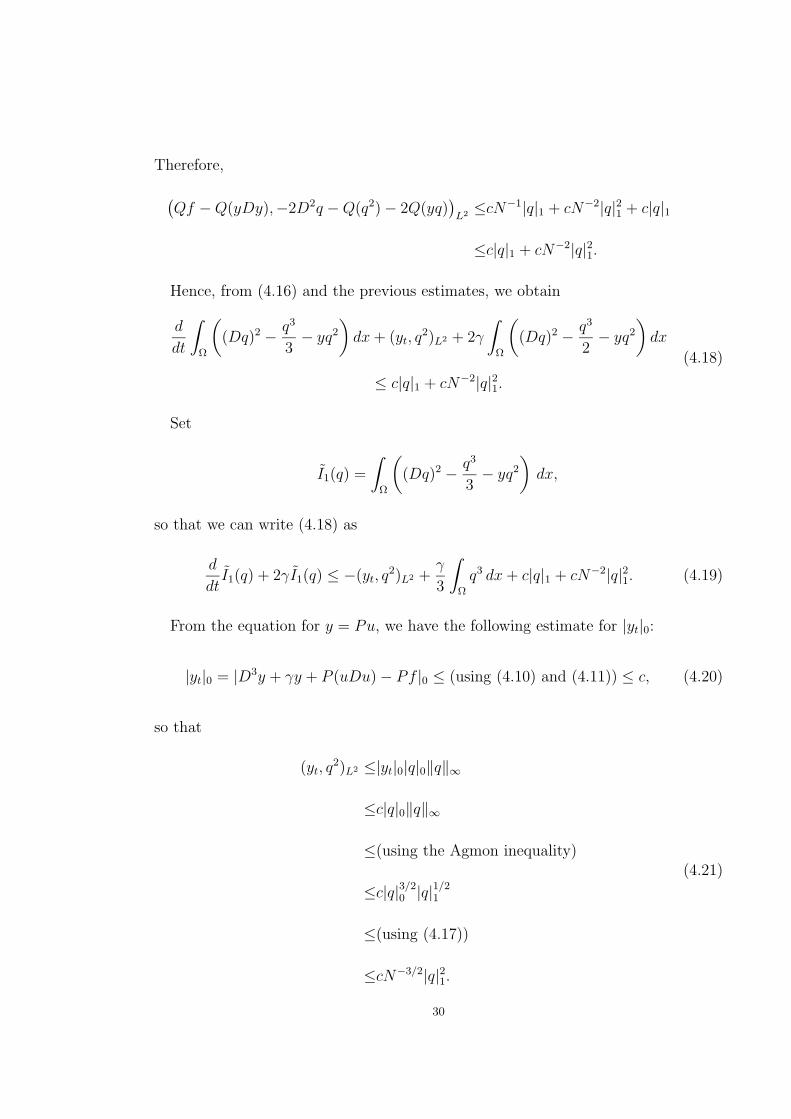
Hence, from (4.16) and the previous estimates, we obtain

d

dt

∫Ω

((Dq)2 − q3

3− yq2

)dx+ (yt, q

2)L2 + 2γ

∫Ω

((Dq)2 − q3

2− yq2

)dx

≤ c|q|1 + cN−2|q|21.(4.18)

Set

I1(q) =

∫Ω

((Dq)2 − q3

3− yq2

)dx,

so that we can write (4.18) as

d

dtI1(q) + 2γI1(q) ≤ −(yt, q

2)L2 +γ

3

∫Ω

q3 dx+ c|q|1 + cN−2|q|21. (4.19)

From the equation for y = Pu, we have the following estimate for |yt|0:

|yt|0 = |D3y + γy + P (uDu)− Pf |0 ≤ (using (4.10) and (4.11)) ≤ c, (4.20)

so that

(yt, q2)L2 ≤|yt|0|q|0‖q‖∞

≤c|q|0‖q‖∞

≤(using the Agmon inequality)

≤c|q|3/20 |q|1/21

≤(using (4.17))

≤cN−3/2|q|21.

(4.21)

30

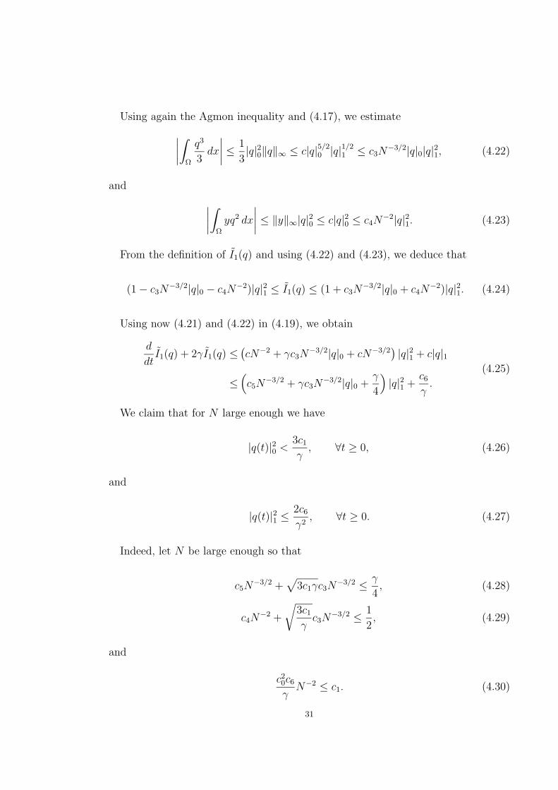
Using again the Agmon inequality and (4.17), we estimate∣∣∣∣∫Ω

q3

3dx

∣∣∣∣ ≤ 1

3|q|20‖q‖∞ ≤ c|q|5/20 |q|

1/21 ≤ c3N

−3/2|q|0|q|21, (4.22)

and ∣∣∣∣∫Ω

yq2 dx

∣∣∣∣ ≤ ‖y‖∞|q|20 ≤ c|q|20 ≤ c4N−2|q|21. (4.23)

From the definition of I1(q) and using (4.22) and (4.23), we deduce that

(1− c3N−3/2|q|0 − c4N

−2)|q|21 ≤ I1(q) ≤ (1 + c3N−3/2|q|0 + c4N

−2)|q|21. (4.24)

Using now (4.21) and (4.22) in (4.19), we obtain

d

dtI1(q) + 2γI1(q) ≤

(cN−2 + γc3N

−3/2|q|0 + cN−3/2)|q|21 + c|q|1

≤(c5N

−3/2 + γc3N−3/2|q|0 +

γ

4

)|q|21 +

c6

γ.

(4.25)

We claim that for N large enough we have

|q(t)|20 <3c1

γ, ∀t ≥ 0, (4.26)

and

|q(t)|21 ≤2c6

γ2, ∀t ≥ 0. (4.27)

Indeed, let N be large enough so that

c5N−3/2 +

√3c1γc3N

−3/2 ≤ γ

4, (4.28)

c4N−2 +

√3c1

γc3N

−3/2 ≤ 1

2, (4.29)

and

c20c6

γN−2 ≤ c1. (4.30)

31

From (4.15) we obtain

|q(t)|20 ≤c1

c2

ec2t <3c1

γ, for 0 ≤ t < t, (4.31)

where t = (1/c2) log(3c2/γ) (recall that c2 ≥ γ, so that 3c2/γ ≥ 3 > 1). Set now

T = sup

t ≥ 0; |q(t)|20 <

3c1

γ

.

Clearly T ≥ t > 0. We want to show that T =∞.

Below, consider t such that 0 ≤ t < T . For such t, we have

|q(t)|20 <3c1

γ, (4.32)

so that from (4.24) and (4.29) we deduce that

1

2|q|21 ≤ I1(q) ≤ 3

2|q|21, (4.33)

while from (4.25) and (4.28) we have

d

dtI1(q) + 2γI1(q) ≤ γ

2|q|21 +

c6

γ. (4.34)

Using now (4.33) and (4.34), we obtain

d

dtI1(q) + γI1(q) ≤ c6

γ, for 0 ≤ t < T. (4.35)

Hence, by the Gronwall Lemma,

I1(q(t)) ≤ I1(q(0))e−γt +c6

γ2=c6

γ2, for 0 ≤ t < T, (4.36)

since q(0) = 0.

Thus, from (4.36) and (4.33), we deduce that

|q(t)|21 ≤ 2I1(q(t)) ≤ 2c6

γ2, for 0 ≤ t < T. (4.37)

32

If T were finite, we would integrate (4.14) on [T − ε, T + ε], for some ε > 0, to find

|q(T + ε)|20 ≤ |q(T − ε)|20e2c2ε +c1

c2

(e2c2ε − 1). (4.38)

But from (4.17) and (4.37) we have

|q(T − ε)|20 ≤c20N−2|q(T − ε)|21

≤2c20c6

γ2N−2

≤(using (4.30))

≤2c1

γ.

(4.39)

Then, from (4.38) and (4.39), we would infer that

|q(T + ε)|20 ≤(

2c1

γ+c1

c2

)e2c2ε − c1

c2

<3c1

γ, for ε ∈

(0,

1

2c2

log3c2 + γ

2c2 + γ

),

contradicting the maximality of T . Therefore, T =∞ and

|q(t)|20 <3c1

γ, ∀t ≥ 0,

and then from (4.37),

|q(t)|21 ≤2c6

γ2, ∀t ≥ 0,

which proves the claim and gives a priori estimates for q in L2(Ω) and H1per(Ω).

Step II. Estimates for q in H2per(Ω).

Multiply the q-equation (4.5) by a special multiplier, namely L2(q) − a2D(yDq),

where a2 is a constant which will be specified in the sequel.

For m = 2 one can find that (2.8) and (2.7) can be written respectively as

L2(q) = 2D4q − α2(Dq)2 + 2α2qD2q + 4δq3, (4.40)

33

and

I2(q) =

∫Ω

((D2q)2 − α2q(Dq)

2 + δq4)dx, (4.41)

for appropriate real numbers α2 and δ (see [5]). From (2.9) and (2.10),

(qt, L2(q))L2 =d

dtI2(q),

and

(D3q + qDq, L2(q))L2 = 0.

Therefore, we obtain

d

dtI2(q) + (qt,−a2D(yDq))L2 + 2γI2(q) + γ(q,−a2D(yDq))L2 − (P (qDq), L2(q))L2

+ (D3q +Q(qDq),−a2D(yDq))L2 + (QD(yq), L2(q)− a2D(yDq))L2

= K2(q) + (Qf,−a2D(yDq))L2 − (Q(yDy), L2(q)− a2D(yDq))L2 ,

(4.42)

where

K2(q) =

∫Ω

(2QD2fD2q − α2f(Dq)2 − 2α2qDqQDf

+ 4δQfq3 + γα2q(Dq)2 − 2γδq4

)dx.

(4.43)

Note that

(qt,−a2D(yDq))L2 = a2(Dqt, yDq) =a2

2

d

dt

∫Ω

(Dq)2y dx− a2

2(yt, (Dq)

2)L2 , (4.44)

and

(D3q,−a2D(yDq))L2 =a2(D2q,D2(yDq))L2

=a2(D2q, yD3q + 2DyD2q +D2yDq)L2

=3a2

2

∫Ω

(D2q)2Dy dx+ a2(D2q,D2yDq)L2 .

(4.45)

34

Also, we have from (QD(yq), L2(q))L2 the term

(QD(yq), 2D4q)L2 =2(D2q,D3(yq))L2

=2(D2q, yD3q + 3DyD2q + 3D2yDq + qD3y)L2

=5

∫Ω

(D2q)2Dy dx+ 6(D2q,D2yDq)L2 + 2(D2q, qD3y)L2 .

(4.46)

Now, we choose a2 = −10/3 in order to cancel the term ((D2q)2, Dy)L2 , which we

cannot control. Using (4.44)-(4.46) in (4.42), we then obtain

d

dt

(I2(q)− 5

3

∫Ω

(Dq)2y dx

)+ 2γ

(I2(q)− 5

3

∫Ω

(Dq)2y dx

)+

5

3(yt, (Dq)

2)L2 + (−10

3+ 6)

∫Ω

D2qDqD2y dx

+ 2

∫Ω

qD2qD3y dx− (P (qDq), L2(q))L2 + (Q(qDq),10

3D(yDq))L2

+ (QD(yq), α2(Dq)2 + 2α2qD2q + 4δq3 +

10

3D(yDq))L2

= K2(q) + (Qf,10

3D(yDq))L2 − (Q(yDy), L2(q) +

10

3D(yDq))L2 .

(4.47)

We estimate below the terms in (4.47) using extensively (4.26) and (4.27) and the

fact that q has zero average, in which case |q|0, |q|1 ≤ c|q|2. We proceed as follows:

(yt, (Dq)2)L2 ≤ |yt|0|q|1‖Dq‖∞ ≤ (using also (4.20)) ≤ c|q|1|q|2 ≤ c|q|2; (4.48)∣∣∣∣∫

Ω

D2qDqD2y dx

∣∣∣∣ ≤|q|2|q|1‖D2y‖∞ ≤ c|q|2|q|1‖y‖3

≤(using (4.27)) ≤ c|q|2;

(4.49)

∣∣∣∣∫Ω

qD2qD3y dx

∣∣∣∣ ≤|q|2‖q‖∞|y|3 ≤ c|q|2|q|1/21 |q|1/20

≤(using (4.26) and (4.27)) ≤ c|q|2;

(4.50)

35

(P (qDq), L2(q))L2 =(P (qDq), 2D4q + α2(Dq)2 + 2α2qD

2q + 4δq3)L2

=(because P and Q are orthogonal)

=(P (qDq), α2(Dq)2 + 2α2qD

2q + 4δq3)L2

≤c|qDq|0(|(Dq)2|0 + |qD2q|0 + |q3|0

)≤c‖q‖∞|q|1

(|q|1‖Dq‖∞ + ‖q‖∞|q|2 + ‖q‖2

∞|q|0)

≤c|q|2;

(4.51)

(Q(qDq),

10

3D(yDq)

)L2

≤c|qDq|0|D(yDq)|0

≤c‖q‖∞|q|1‖y‖1|q|2 ≤ c|q|2;

(4.52)

and (QD(yq), α2(Dq)2 + 2α2qD

2q + 4δq3 +10

3D(yDq)

)L2

≤ c|D(yq)|0(|(Dq)2|0 + |qD2q|0 + |q|30 + |D(yDq)|0

)≤ c‖y‖1|q|1

(|q|1‖Dq‖∞ + ‖q‖∞|q|2 + ‖q‖2

∞|q|0 + ‖y‖1|q|2)

≤ c|q|2.

(4.53)

For the right hand side terms in (4.47) we have the following estimates:

K2(q) ≤2|Qf |2|q|2 + c‖f‖∞|q|1 + c|q|0|q|1‖QDf‖∞

+ c‖Qf‖∞‖q‖∞|q|20 + c‖q‖∞|q|21 + c‖q‖2∞|q|20

≤c|q|2;

(4.54)

(Qf,

10

3D(yDq)

)L2

≤c|Qf |0|D(yDq)|0 ≤ c|Qf |0‖y‖1|q|2

≤c|q|2;

(4.55)

36

and(Q(yDy), L2(q) +

10

3D(yDq)

)L2

= 2(D2(yDy), D2q)L2 +

(Q(yDy), α2(Dq)2 + 2α2qD

2q + 4δq3 +10

3D(yDq)

)L2

≤ c|D2(yDy)|0|q|2 + c|q|2

≤ c‖y‖3‖y‖2|q|2 + c|q|2

≤ c|q|2.

(4.56)

Using now (4.48)-(4.56) in (4.47), we obtain

d

dt

(I2(q)− 5

3

∫Ω

(Dq)2y dx

)+ 2γ

(I2(q)− 5

3

∫Ω

(Dq)2y dx

)≤ c|q|2 ≤ γ|q|22 + c.

(4.57)

Consider now∣∣∣∣∫Ω

(−α2(Dq)2 + δq4 − 5

3(Dq)2y) dx

∣∣∣∣ ≤c (|q|21 + ‖q‖2∞|q|20 + |q|1‖y‖∞

)≤(using again (4.26) and (4.27)) ≤ c,

(4.58)

so that

|q|22 − c ≤ I2(q)− 5

3

∫Ω

(Dq)2y dx ≤ |q|22 + c. (4.59)

Then, from (4.57) and (4.59), we obtain

d

dt

(I2(q)− 5

3(Dq)2y dx

)+ γ

(I2(q)− 5

3

∫Ω

(Dq)2y dx

)≤ c, ∀t ≥ 0.

Therefore, since q(0) = 0, we find that

I2(q(t))− 5

3

∫Ω

(Dq(t))2y(t) dx ≤ c, ∀t ≥ 0,

37

which, together with (4.59), gives

|q(t)|22 ≤ c, ∀t ≥ 0. (4.60)

Step III. Estimates for q in Hkper(Ω).

Multiply the q-equation (4.5) by

2(−1)kD2kq + ak(−1)k−1Dk−1(yDk−1q),

where ak will be specified later on. We obtain

d

dt

(|q|2k +

ak2

∫Ω

(Dk−1q)2y dx

)− ak

2

∫Ω

(Dk−1q)2yt dx

+(D3q, ak(−1)k−1Dk−1(yDk−1q)

)L2 + 2γ

(|q|2k +

ak2

∫Ω

(Dk−1q)2y dx

)+(Q(qDq), 2(−1)kD2kq + ak(−1)k−1Dk−1(yDk−1q)

)L2

+(Q(D(yq)), 2(−1)kD2kq + ak(−1)k−1Dk−1(yDk−1q)

)L2

=(Qf −Q(yDy), 2(−1)kD2kq + ak(−1)k−1Dk−1(yDk−1q)

)L2 .

(4.61)

Note that

(D3q, ak(−1)k−1Dk−1(yDk−1q)

)L2

=(Dkq, akD

2(yDk−1q))L2

=

∫Ω

akDkq(yDk+1q + 2DkqDy +Dk−1qD2y

)dx

=3ak2

∫Ω

(Dkq)2Dy dx+ ak

∫Ω

DkqDk−1qD2y dx,

(4.62)

38

and

(Q(D(yq), 2(−1)kD2kq

)L2

=(D(yq), 2(−1)kD2kq

)L2

= 2(Dk+1(yq), Dkq

)L2

= 2

(Dkq,

k+1∑j=0

(k + 1

j

)Dk+1−jqDjy

)L2

= (2k + 1)

∫Ω

(Dkq)2Dy dx+ 2k+1∑j=2

(k + 1

j

)(Dkq,Dk+1−jqDjy

)L2 .

(4.63)

We pass now to the estimates in (4.61), taking (4.62) and (4.63) into account. We

first have

∣∣∣∣∫Ω

DkqDk−1qD2y dx

∣∣∣∣ ≤|q|k|q|k−1‖D2y‖∞

≤c|q|k|q|k−1‖y‖3 ≤ c|q|k|q|k−1

≤(using (4.3)) ≤ cN−1|q|2k.

(4.64)

39

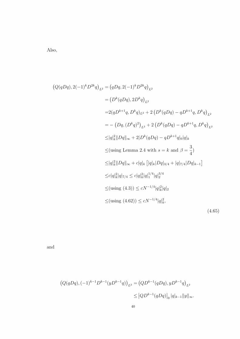
Also,

(Q(qDq), 2(−1)kD2kq

)L2 =

(qDq, 2(−1)kD2kq

)L2

=(Dk(qDq), 2Dkq

)L2

=2(qDk+1q,Dkq)L2 + 2(Dk(qDq)− qDk+1q,Dkq

)L2

=−(Dq, (Dkq)2

)L2 + 2

(Dk(qDq)− qDk+1q,Dkq

)L2

≤|q|2k‖Dq‖∞ + 2|Dk(qDq)− qDk+1q|0|q|k

≤(using Lemma 2.4 with s = k and β =3

4)

≤|q|2k‖Dq‖∞ + c|q|k[|q|k|Dq|3/4 + |q|7/4|Dq|k−1

]≤c|q|2k|q|7/4 ≤ c|q|2k|q|

1/41 |q|

3/42

≤(using (4.3)) ≤ cN−1/4|q|2k|q|2

≤(using (4.62)) ≤ cN−1/4|q|2k,

(4.65)

and

(Q(qDq), (−1)k−1Dk−1(yDk−1q)

)L2 =

(QDk−1(qDq), yDk−1q

)L2

≤∣∣QDk−1(qDq)

∣∣0|q|k−1‖y‖∞.

40

Since

|QDk−1(qDq)|0 ≤|Dk−1(qDq)|

≤|qDkq|0 + |Dk−1(qDq)− qDkq|0

≤(using Lemma 2.4 with s = k − 1 and β = 1)

≤‖q‖∞|q|k + c (|q|k−1|Dq|1 + |q|2|Dq|k−2)

≤c|q|1|q|k + c|q|k−1|q|2

≤(using (4.60))

≤c|q|k + c|q|k−1 ≤ c|q|k,

we also have(Q(qDq), (−1)k−1Dk−1(yDk−1q)

)L2 ≤c|q|k|q|k−1‖y‖∞

≤c|q|k|q|k−1 ≤ (using (4.3))

≤cN−1|q|2k.

(4.66)

Now, consider the remaining terms from (QD(yq), 2(−1)kD2kq)L2 in (4.63):∣∣∣∣∣k+1∑j=2

(k + 1

j

)∫Ω

Dk+1−jqDkqDjy dx

∣∣∣∣∣ ≤c|q|k(k+1∑j=2

|q|k+1−j‖Djy‖∞

)

≤c|q|k

(k+1∑j=2

|q|k+1−j‖y‖j+1

)

≤(using (4.1) and (4.3))

≤c|q|k

(k+1∑j=2

N−j+1|q|kN j−2‖y‖3

)

≤(using (4.11))

≤cN−1|q|2k.

(4.67)

41

We also have

(QD(yq), (−1)k−1Dk−1(yDk−1q)

)=(QDk(yq), yDk−1q

)L2

≤|QDk(yq)|0|q|k−1‖y‖∞.

But as in (4.67), we can estimate

|QDk(yq)|0 ≤|Dk(yq)|0 ≤ c

k∑j=0

|Dk−jqDjy|0

≤ck∑j=0

|q|k−j‖Djy‖∞

≤c

(|q|k‖y‖∞ + |q|k−1‖Dy‖∞ +

k∑j=2

N−j|q|kN j−2‖y‖3

)

≤c|q|k.

Hence,

(QD(yq), (−1)k−1Dk−1(yDk−1q)

)L2 ≤c|q|k|q|k−1‖y‖∞

≤c|q|k|q|k−1

≤cN−1|q|2k.

(4.68)

Moreover, using the Agmon inequality, (4.20), and (4.3),

(yt, (D

k−1q)2)L2 ≤|yt|0|q|k−1‖Dk−1q‖∞

≤c|yt|0|q|3/2k−1|q|1/2k

≤cN−3/2|q|2k.

(4.69)

42

For the right hand side of (4.61) we proceed as follows:

(Qf, 2(−1)kD2kq + ak(−1)k−1Dk−1(yDk−1q)

)L2

≤ (2QDkf,Dkq)L2 + (QDk−1f, akyDk−1q)L2

≤ 2|Qf |k|q|k + c|Qf |k−1|q|k−1‖y‖∞

≤ c|q|k + c|q|k−1 ≤ c|q|k,

(4.70)

and

(Q(yDy), 2(−1)kD2kq + ak(−1)k−1Dk−1(yDk−1q)

)L2

= 2(QDk(yDy), Dkq)L2 + ak(QDk−1(yDy), yDk−1q)L2

≤ 2|QDk(yDy)|0|q|k + c|QDk−1(yDy)|0|q|k−1‖y‖∞,

but

|QDk(yDy)|0 ≤|Dk(yDy)|0 ≤ |yDk+1y|0 + |Dk(yDy)− yDk+1y|0

≤(using again Lemma 2.4 with s = k and β = 1)

≤|y|k+1‖y‖∞ + c (‖y‖k‖Dy‖1 + ‖y‖2‖Dy‖k−1)

≤|y|k+1‖y‖∞ + c‖y‖k‖y‖2

≤c‖y‖k+1 + c‖y‖k ≤ (using (4.12) and (4.11))

≤cNk−2‖y‖3 + cNk−3‖y‖3 ≤ cNk−2,

and, similarly,

|QDk−1(yDy)|0 ≤ cNk−3,

43

so that (Q(yDy), 2(−1)kD2kq + ak(−1)k−1Dk−1(yDk−1q)

)L2

≤ cNk−2|q|k + cNk−3|q|k−1‖y‖∞

≤ (using (4.3)) ≤ cNk−2|q|k.

(4.71)

Choose now ak = −2(2k+ 1)/3 in order to cancel the term ((Dkq)2, Dy)L2 . Then,

using the estimates (4.64)-(4.71) in (4.61), we obtain

d

dt

(|q|2k −

2k + 1

3

∫Ω

(Dk−1q)2y dx

)+ 2γ

(|q|2k −

2k + 1

3

∫Ω

(Dk−1q)2y dx

)≤ cNk−2|q|k + c7N

−1/4|q|2k

≤ γ

4|q|2k + cN2(k−2) + c7N

−1/4|q|2k.

(4.72)

Note now that for some constant c8,∣∣∣∣2k + 1

3

∫Ω

(Dk−1q)2y dx

∣∣∣∣ ≤ c|q|2k−1‖y‖∞ ≤ c8N−2|q|2k.

Assume that N is large enough so that

c8N−2 ≤ 1

2(4.73)

and

c7N−1/4 ≤ γ

4. (4.74)

Then, we find

1

2|q|2k ≤ |q|2k −

2k + 1

3

∫Ω

(Dk−1q)2y dx ≤ 3

2|q|2k, (4.75)

which gives in (4.72) that

d

dt

(|q|2k −

2k + 1

3

∫Ω

(Dk−1q)2y dx

)+ γ

(|q|2k −

2k + 1

3

∫Ω

(Dk−1q)2y dx

)≤ cN2(k−2), ∀t ≥ 0.

(4.76)

44

Therefore, by the Gronwall Lemma,

|q(t)|2k −2k + 1

3

∫Ω

(Dk−1q)2y dx ≤(|q(0)|2k −

2k + 1

3

∫Ω

(Dk−1q(0))2y(0) dx

)e−γt

+ cN2(k−2)

=cN2(k−2), ∀t ≥ 0.

From this relation and (4.75), we deduce that

|q(t)|k ≤ cNk−2, ∀t ≥ 0, (4.77)

for N satisfying (4.28)-(4.30), (4.73) and (4.74).

Thus, we have proved (4.8).

Step IV. Decay of z in H1per(Ω).

Using (4.77) for k = 3 and the q-equation (4.5) we deduce that

|qt|0 ≤ cN, ∀t ≥ 0,

which, together with (4.20), implies the following estimates for v = y + q:

|vt|0 ≤ cN, ∀t ≥ 0, (4.78)

and

‖v(t)‖2 ≤ c, ∀t ≥ 0, (4.79)

Also, note that q + z solves the same equation as QNu, so that by uniqueness we

have q + z = QNu. Therefore, from (4.10) and the previous Step I, we find that

|z(t)|0 = |QNu(t)− q(t)|0 ≤ |u(t)|0 + |q(t)|0 ≤ c9, ∀t ≥ 0. (4.80)

45

Multiply now the z-equation (4.6) by −2D2z − Q(z2) − 2Q(vz). Similar compu-

tations as those for q yield

d

dt

∫Ω

((Dz)2 − z3

3− vz2

)dx+ 2γ

∫Ω

((Dz)2 − z3

3− vz2

)dx

+ (vt, z2)L2 − γ

3

∫Ω

z3 dx = 0.

(4.81)

We estimate

(vt, z2)L2 ≤|vt|0|z|0‖z‖∞ ≤ c|vt|0|z|3/20 |z|

1/21

≤(using (4.3) and (4.78))

≤cNN−3/2|z|21 = c10N−1/2|z|21,

(4.82)

and∣∣∣∣∫Ω

z3

3dx

∣∣∣∣ ≤ 1

3|z|20‖z‖∞ ≤ c|z|5/20 |z|

1/21 ≤ (using (4.3) and (4.80)) ≤ c11N

−3/2|z|21,

(4.83)

and also∣∣∣∣∫Ω

vz2 dx

∣∣∣∣ ≤ ‖v‖∞|z|20 ≤ c‖v‖1|z|20 ≤ (using (4.3) and (4.79)) ≤ c12N−2|z|21. (4.84)

We claim that for N large enough we have

|z(t)|21 ≤ ce−γt, ∀t ≥ 0, (4.85)

for some constant c.

Indeed, let N be large enough so that

c11N−3/2 + c12N

−2 ≤ 1

2, (4.86)

c10N−1/2 + γc11N

−3/2 ≤ γ

2. (4.87)

46

Using (4.83), (4.84), and (4.86), we deduce that

1

2|z|21 ≤ |z|21 −

∫Ω

z3

3dx+

∫z2v dx ≤ 3

2|z|21. (4.88)

Now, using (4.81), (4.82), (4.87), and (4.88), we obtain

d

dt

∫Ω

((Dz)2 − z3

3+ z2v

)dx+ 2γ

∫Ω

((Dz)2 − z3

3+ z2v

)dx

≤ γ

2|z|21

≤ γ

∫Ω

((Dz)2 − z3

3+ z2v

)dx,

and, hence,

d

dt

(∫Ω

((Dz)2 − z3

3+ z2v

)dx

)+ γ

∫Ω

((Dz)2 − z3

3+ z2v

)dx ≤ 0. (4.89)

Therefore, by the Gronwall Lemma,

|z(t)|21 −∫

Ω

(z(t))3

3dx+

∫Ω

(z(t))2v(t) dx

≤(|z(0)|21 −

∫Ω

(z(0))3

3dx+

∫Ω

(z(0))2v(0) dx

)e−γt, ∀t ≥ 0.

(4.90)

From (4.90) and (4.88), we deduce that

|z(t)|21 ≤ 3|z(0)|21e−γt, ∀t ≥ 0. (4.91)

Now, since z has zero average, the norm ‖ · ‖1 is equivalent to | · |1. Therefore, we

deduce from (4.91) that

‖z(t)‖21 ≤ ce−γt, ∀t ≥ 0. (4.92)

This finishes the proof of Proposition 4.1.

Thanks to Proposition 4.1, we can define the families S(3)1 (t)t≥0 and S(3)

2 (t)t≥0

of maps in H3per(Ω) given by

S(3)1 (t)u0 = y(t) + q(t) and S

(3)2 (t)u0 = z(t), ∀t ≥ 0, (4.93)

47

where y(t) = PNS(3)(t)u0 = PNu(t), and q and z are respectively the solutions of

problems (4.5) and (4.6) for a given u0 in H3per(Ω).

Note then that w = q + z is a solution of the following problem:dw

dt+D3w + γw +QN((y + w)D(y + w)) = QNf,

w(0) = QNu0.

(4.94)

Since QNu is also a solution of this problem, it follows by uniqueness that QNu =

q + z. In other words, we have that

S(3)(t) = S(3)1 (t) + S

(3)2 (t), ∀t ≥ 0, (4.95)

as operators defined in H3per(Ω).

We are now in position to show that A3 = Ak. Consider then u ∈ A3. From (3.31)

and a well-known characterization of ω-limit sets, there exist a sequence of elements

un ∈ B3 and a sequence of positive real numbers tn which tends to infinity as n goes

to infinity such that

S(3)(tn)un → u, in H3per(Ω), as n→∞. (4.96)

We also have from (4.95) that

S(3)(tn)un = S(3)1 (tn)un + S

(3)2 (tn)un, ∀n ∈ N. (4.97)

From the definition (4.93) and using (4.8), (4.9), and (4.11), we deduce that if N

is large enough (given by Proposition 4.1), then

‖S(3)1 (tn)un‖k ≤ cNk−2, ∀n ∈ N, (4.98)

and

‖S(3)2 (tn)un‖1 ≤ ce−

γ2tn , ∀n ∈ N, (4.99)

48

for some constant c.

From (4.98) we infer that there exist subsequences tn′ and un′ , and w ∈ Hkper(Ω)

such that

S(3)1 (tn′)un′ w, weakly in Hk

per(Ω). (4.100)

We also have

‖w‖k ≤ lim infn′→∞

‖S(3)1 (tn′)un′‖k ≤ cNk−2. (4.101)

Consider v ∈ L2(Ω). From (4.97) we can write

(S(3)(tn′)un′ , v

)L2 =

(S

(3)1 (tn′)un′ , v

)L2

+(S

(3)2 (tn′)un′ , v

)L2.

Passing the expression above to the limit n′ → ∞ and using (4.96), (4.99), and

(4.100) we obtain

(u, v)L2 = (w, v)L2 , ∀v ∈ L2(Ω).

Therefore, u = w in L2(Ω) and, consequently, u ∈ Hkper(Ω). From (4.101), we also

have

‖u‖k ≤ cNk−2, ∀u ∈ A3.

In other words, A3 is contained and bounded in Hkper(Ω). Since Ak attracts all

bounded sets in Hkper(Ω), we have, moreover,

distHk(A3,Ak) = distHk(S(k)(t)A3,Ak)→ 0, as t→∞.

Hence,

A3 ⊂ AkHk

per(Ω)= Ak.

Thus, we have proved the following result:

49

Theorem 4.2. Let f ∈ Hkper(Ω), k ≥ 4 and γ > 0 be given. Then A3 = A4 = · · · =

Ak, where A3, . . . ,Ak are the global attractors obtained in Theorem 3.2.

Remark 4.1. Note that Theorem 4.2 is a regularity result; it says that the global

attractors Aj for S(j)(t)t∈R with j ≥ 3 are as smooth as the forcing term.

Remark 4.2. For regularity reasons, we were not able to prove that A2 = A3 using

the techniques above.

5. Appendix to Section 2

In this section we prove the results stated in Section 2.

Proof of Theorem 2.1. The proof is by parabolic regularization as in [18]. We con-

sider for ε ∈ (0, 1] the following problem:

duεdt

+ uεDuε +D3uε + γuε + εD4uε = fε, (5.1)

uε(0) = u0ε, (5.2)

where fε and uε are respectively approximations in Hkper(Ω) of f and u0 by smooth

(C∞ and L-periodic) functions.

It is classical to deduce that there exists uε = uε(t), t ∈ [0,∞), satisfying (5.1)

and (5.2) and also

uε ∈ L∞(0, T ;L2(Ω)) ∩ L2(0, T ;H2per(Ω)), ∀T > 0. (5.3)

Then, Duε ∈ L2(0, T ;H1per(Ω)) ⊂ L2(0, T ;L∞(Ω)), so that uεDuε ∈ L2(0, T ;L2(Ω)).

Hence,

duεdt

+D3uε + γuε + εD4uε = fε − uεDuε ∈ L2(0, T ;L2(Ω)). (5.4)

50

By a classical regularity result for linear parabolic equations we obtain

uε ∈ L2(0, T ;H4per(Ω)),

duεdt∈ L2(0, T ;L2(Ω)). (5.5)

We remark that the right-hand side in (5.4) is actually more regular and we deduce

that uε is also more regular. We can continue this reasoning indefinitely to conclude

that uε is C∞ in (0,∞)× Ω. Hence, all the computations below will be justified.

We need now prove that uε remains bounded in L∞(0, T ;Hkper(Ω)) as ε goes to 0.

First, we find estimates for uε independent of ε in L∞(0, T ;H2per(Ω)). Using these esti-

mates it will be easy to obtain estimates for uε independent of ε in L∞(0, T ;Hkper(Ω)).

Since we are now interested in finite time estimates, we fix T > 0 and let c denote a

generic constant independent of ε, but which might depend on T and the other data

(including k). We will use the fact that u0ε and fε converge respectively to u0 and

f in Hkper(Ω), so that we can bound ‖u0ε‖k and ‖fε‖k independently of ε. We also

note that all the estimates obtained will be uniformly valid for ‖u0‖k bounded.

Step I. Estimates for uε in L∞(0, T ;H2per(Ω)).

First, multiply equation (5.1) by L0(uε) = 2uε and integrate the result on Ω. We

find

d

dt|uε|20 + 2γ|uε|20 + 2ε|D2uε|20 =2

∫Ω

fεuε dx

≤2|fε|0|uε|0

≤|γ||uε|20 +1

|γ||fε|20.

(5.6)

Hence,

d

dt|uε|20 + 2ε|D2uε|20 ≤ 3|γ||uε|20 +

1

|γ||fε|20.

51

By multiplying the above expression by exp(−3|γ|t) and integrating it on t, we obtain

|uε(t)|20 + 2ε

∫ t

0

|uε(s)|22 ds ≤ |u0ε|20e3|γ|t +|fε|203γ2

e3|γ|t,

so that for 0 ≤ t ≤ T ,

|uε(t)|20 + ε

∫ t

0

|uε(s)|22 ds ≤ c, (5.7)

for some constant c > 0.

Multiplying now equation (5.1) by L1(uε) = −2D2uε − u2ε, we find that

d

dt

∫Ω

((Duε)

2 − 1

3u3ε

)dx+ 2γ

∫Ω

((Duε)

2 − 1

2u3ε

)dx

+ 2ε

∫Ω

((D3uε)

2 + uεDuεD3uε)dx

=

∫Ω

(2DfεDuε − fεu2

ε

)dx.

(5.8)

Using now (3.7), (3.8) and (5.7), we can write for 0 ≤ t ≤ T that

γ

3

∫Ω

u3ε dx ≤

|γ|2

∫Ω

((Duε)

2 − 1

3u3ε

)dx+ c. (5.9)

Now we have∣∣∣∣2∫Ω

uεDuεD3uε dx

∣∣∣∣ ≤2‖uε‖L4‖Duε‖L4|D3uε|0

≤c‖uε‖H1/4‖Duε‖H1/4 |D3uε|0

≤(by interpolation inequalities)

≤c|uε|3/20 ‖uε‖1/23 |uε|3

≤c|uε|20|uε|3 + c|uε|3/20 |uε|3/23

≤|uε|23 + c|uε|40 + c|uε|60

≤(using (5.7))

≤|uε|23 + c, for 0 ≤ t ≤ T.

(5.10)

52

We also have∣∣∣∣∫Ω

(2DfεDuε − fεu2

ε

)dx

∣∣∣∣ ≤2|fε|1|uε|1 + ‖fε‖∞|uε|20

≤|γ|3|uε|21 +

3

|γ||fε|21 + ‖fε‖∞|uε|20

≤(using (5.7) and (3.8))

≤|γ|2I1(uε) + c, for 0 ≤ t ≤ T,

(5.11)

where

I1(uε) =

∫Ω

((Duε)

2 − 1

3u3ε

)dx.

Inserting (5.9), (5.10), and (5.11) in (5.8), we obtain

d

dtI1(uε) + 2γI1(uε) + ε|uε|23 ≤ |γ|I1(uε) + c, for 0 ≤ t ≤ T.

But from (3.8), (3.9), and (5.7) we find that

2

3|uε|21 − c ≤ I1(uε) ≤

4

3|uε|21 + c, for 0 ≤ t ≤ T,

from where we can deduce that

−2γI1(uε) ≤ 2|γ|I1(uε) + c, for 0 ≤ t ≤ T.

Therefore, we obtain

d

dtI1(uε) + ε|uε|23 ≤ 3|γ|I1(uε) + c, for 0 ≤ t ≤ T, (5.12)

which implies that

I1(uε(t)) + ε

∫ t

0

|uε(s)|23 ds ≤ I1(u0ε)e3|γ|t +

c

3|γ|e3|γ|t, for 0 ≤ t ≤ T. (5.13)

Using (3.8) and (3.9) we deduce from (5.13) that

|uε(t)|21 + ε

∫ t

0

|uε(s)|23 ds ≤ c, for 0 ≤ t ≤ T. (5.14)

53

A simple computation using the method of undetermined coefficients described in

Section 2 yields

L2(uε) = 2D4uε +5

3(Duε)

2 +10

3uεD

2uε +5

9u3ε, (5.15)

and

I2(uε) =

∫Ω

((D2uε)

2 − 5

3(Duε)

2 +5

36u4ε

)dx. (5.16)

Multiply the regularized equation (5.1) by L2(uε) to find that

d

dtI2(uε) + 2γI2(uε)

+ ε

∫Ω

(2(D4uε)

2 +5

3(Duε)

2D4uε +10

3uεD

2uεD4uε +

5

9u3εD

4uε

)dx

=

∫Ω

(2D2fεD

2uε +5

3(Duε)

2fε +10

3uεD

2uεfε +5

9u3εfε

)dx

+ γ

∫Ω

(5

3uε(Duε)

2 − 5

18u4ε

)dx.

(5.17)

We estimate now the terms in (5.17). First,

∣∣∣∣γ ∫Ω

(5

3uε(Duε)

2 − 5

18u4ε

)dx

∣∣∣∣ ≤c‖uε‖∞|uε|21 + c‖uε‖2∞|uε|20

≤(using (2.6), (5.7) and (5.14))

≤c, for 0 ≤ t ≤ T.

(5.18)

54

Using the continuous imbeddings H1per(Ω) ⊂ L∞(Ω) and H1/4(Ω) ⊂ L4(Ω), (5.7),

and (5.14), we estimate∣∣∣∣∫Ω

(5

3(Duε)

2 +10

3uεD

2uε +5

9u3ε

)D4uε dx

∣∣∣∣≤ c

(‖Duε‖2

H1/4 + ‖uε‖∞|uε|2 + ‖uε‖2∞|uε|0

)|uε|4

≤ c(‖uε‖2

H5/4 + |uε|2 + 1)|uε|4

≤ (by interpolation)

≤ c|uε|11/80 ‖uε‖5/8

4 |uε|4 + c|uε|1/20 ‖uε‖1/24 |uε|4 + c|uε|4

≤ (by the Young inequality)

≤ |uε|24 + c, for 0 ≤ t ≤ T.

(5.19)

We also have∣∣∣∣∫Ω

(2D2fεD

2uε +5

3(Duε)

2fε +10

3uεD

2uεfε +5

9u3εfε

)dx

∣∣∣∣≤ 2|fε|2|uε|2 + c‖fε‖∞|uε|21 + c|fε|1‖uε‖∞|uε|1 + c|fε|0|uε|0‖uε‖2

∞

≤ (using (5.14))

≤ |γ||uε|22 +1

|γ||fε|22 + c, for 0 ≤ t ≤ T.

(5.20)

We deduce from (5.16), (5.7) and (5.14) that

|uε|22 ≤ I2(uε) + c, for 0 ≤ t ≤ T, (5.21)

and also

|I2(uε)| ≤ |uε|22 + c ≤ (by (5.21)) ≤ I2(uε) + c, for 0 ≤ t ≤ T. (5.22)

Using (5.18)-(5.22), we infer from (5.17) that

d

dtI2(uε) + ε|uε|24 ≤ 3|γ|I2(uε) + c, for 0 ≤ t ≤ T. (5.23)

55

Therefore,

I2(uε(t)) + ε

∫ t

0

|uε(s)|24 ds ≤ I2(u0ε)e3|γ|t +

c

3|γ|e3|γ|t, for 0 ≤ t ≤ T,

which, together with (5.21) and (5.22), gives

|uε(t)|22 + ε

∫ t

0

|uε(s)|24 ds ≤ c, for 0 ≤ t ≤ T. (5.24)

Step II. Estimates for uε in L∞(0, T ;Hkper(Ω)), k ≥ 2.

Since we are now only interested in finite-time estimates, we can use Lemma

2.4 and the estimates (5.7), (5.14), and (5.24) in order to obtain estimates for uε

independent of ε in Hkper(Ω), for k ≥ 2, avoiding the use of the invariants Ik. Multiply

then equation (5.1) by 2(−1)kD2kuε to find

d

dt|uε|2k + 2

∫Ω

DkuεDk(uεDuε) dx+ 2γ|uε|2k + 2ε|uε|2k+2 = 2

∫Ω

DkfεDkuε dx.

(5.25)

We estimate∣∣∣∣2∫Ω

DkuεDk(uεDuε) dx

∣∣∣∣=

∣∣∣∣2∫Ω

DkuεDk+1uε uε dx+ 2

∫Ω

Dkuε(Dk(uεDuε)− uεDk+1uε

)dx

∣∣∣∣=

∣∣∣∣−∫Ω

(Dkuε)2Duε dx+ 2

∫Ω

Dkuε(Dk(uεDuε)− uεDk+1uε

)dx

∣∣∣∣≤ ‖Duε‖∞|uε|2k + 2|uε|k|Dk(uεDuε)− uεDk+1uε|0

≤ (using Lemma 2.4 with s = k and β = 1)

≤ ‖Duε‖∞|uε|2k + c|uε|k (‖uε‖k‖Duε‖1 + ‖u‖2‖Duε‖k−1)

≤ (using (5.7) and (5.24))

≤ c|uε|2k + c, for 0 ≤ t ≤ T.

(5.26)

56

Hence, we infer from (5.25) that

d

dt|uε|2k + ε|uε|2k+2 ≤ c|uε|2k + c|fε|2k + c, for 0 ≤ t ≤ T. (5.27)

Therefore,

|uε(t)|2k + ε

∫ t

0

|uε(s)|2k+2 ds ≤ c, for 0 ≤ t ≤ T. (5.28)

Now, thanks to (5.7), (5.14), and (5.24), and since

duεdt

= −uεDuε −D3uε − γuε − εD4uε + fε,

we deduce that, for any T > 0,

duεdt

remains bounded in L2(0, T ;H−1(Ω)), (5.29)

where H−1(Ω) denotes the dual space of H1per(Ω) when we identify L2(Ω) with its

dual.

From (5.28) and (5.29), there exist u and a subsequence of uε (still denoted by uε)

such that, for every T > 0,

uε → u in L∞(0, T ;Hkper(Ω)) weak star, (5.30)

and

duεdt→ du

dtin L2(0, T ;H−1(Ω)) weakly, (5.31)

as ε→ 0. Since the imbedding Hkper(Ω) ⊂ Hk−1

per (Ω) is compact, it follows from (5.30)

and (5.31) that

uε → u in L2(0, T ;Hk−1per (Ω)) strongly. (5.32)

Hence,

uεDuε → uDu in L2(0, T ;Hk−1per (Ω)) weakly. (5.33)

57

Then, we can pass to the limit in the equation (5.1) as ε goes to zero to find

du

dt+ uDu+D3u+ γu = f (5.34)

in H−1(Ω) and in particular in the distribution sense in Ω× (0,∞), with u satisfying

u ∈ L∞(0, T ;Hkper(Ω)), ∀T > 0, (5.35)

and

du

dt∈ L∞(0, T ;H−1(Ω)), ∀T > 0. (5.36)

The relation (5.36) follows from (5.35) and (5.34). From (5.35) and (5.36) it follows

by Lemma II.3.2 in [19] that u is almost everywhere equal to a continuous function

from [0, T ] into L2(Ω),

u ∈ C([0, T ], L2(Ω)), ∀T > 0. (5.37)

Similarly, it follows from (5.30) and (5.31) that uε(0) converges to u(0) in L2(Ω),

and since u0ε converges to u0 in Hkper(Ω), we conclude that

u(0) = u0. (5.38)

For the uniqueness, let u and v be two solutions satisfying (5.34), (5.35), and

(5.38). Then, u and v satisfy also (5.36) and (5.37), and w = u− v satisfies (5.35),

(5.36), (5.37), and

dw

dt+D3w + γw = −uDu+ vDv, (5.39)

w(0) = 0. (5.40)

Since w satisfies (5.35) and (5.36), it follows that

1

2

d

dt|w|20 = 〈dw

dt, w〉H−1,H1

per.

58

Then (5.39) implies

1

2

d

dt|w|20 + γ|w|20 = −

∫Ω

(uDu− vDv)w dx.

But note that∫Ω

(uDu− vDv)w dx =

∫Ω

(wDw +D(vw))w dx =

∫Ω

1

2w2Dv dx.

Hence,

d

dt|w|20 =− 2γ|w|20 −

1

2

∫Ω

w2Dv dx

≤1

2‖Dv‖∞|w|20 + 2|γ||w|20

≤(using (5.35))

≤c|w|20.

By the Gronwall Lemma and (5.40) we deduce that w = 0, i.e., u = v, which proves

the uniqueness. Thus, the proof of Theorem 2.1 is complete.

Proof of Theorem 2.2. We consider again the regularized problem (5.1)-(5.2), but we

now take particular regularizations of u0 and f . We consider the Fourier series of u0

and write

u0 =∑j∈Z

uj0e2πijx/L.

For ε ∈ (0, 1], set then

u0ε =∑|j|≤ε−p

uj0e2πjx/L,

where p > 0 will be fixed later on. We have u0ε ∈ C∞per(Ω) since the sum is finite. We

define similarly fε.

We need the following technical result:

59

Lemma 5.1. Let

v =∑j∈Z

vje2πijx/L.

For p > 0 and ε ∈ (0, 1] set

vε =∑|j|≤ε−p

vje2πijx/L.

Then the following estimates hold:

‖vε‖2m+l ≤

(1 + (2π)2l

)ε−2pl‖vε‖2

m, ∀l ≥ 0, (5.41)

and

‖v − vε‖2m−l ≤

(1

2π

)2l

ε2pl‖v − vε‖2m, for 0 ≤ l ≤ m. (5.42)

Proof. We have

‖v‖2m =

m∑n=0

L2n|v|2n,

where

|v|2n =

∫Ω

|Dnv|2 dx = L∑j∈Z

(2πj

L

)2n

|vj|2.

We first obtain

|vε|2m+l =L∑|j|≤ε−p

(2πj

L

)2(m+l)

|vj|2

≤L(

2πε−p

L

)2l ∑|j|≤ε−p

(2πj

L

)2m

|vj|2

=

(2π

L

)2l

ε−2pl|vε|2m.

60

Hence,

‖vε‖2m+l =‖vε‖2

m +m+l∑

n=m+1

L2n|vε|2n

=‖vε‖2m +

m∑n=m−l+1

L2(n+l)|vε|2n+l

≤‖vε‖2m +

m∑n=m−l+1

L2(n+l)

(2π

L

)2l

ε−2pl|vε|2n

=‖vε‖2m + (2π)2lε−2pl

m∑n=m−l+1

L2n|vε|2n

≤(1 + (2π)2lε−2pl

)‖vε‖2

m

≤(1 + (2π)2l

)ε−2pl‖vε‖2

m,

where we used that 0 < ε ≤ 1.

Also,

|v − vε|2m−l =L∑|j|>ε−p

(2πj

L

)2(m−l)

|vj|2

≤L(

2πε−p

L

)−2l ∑|j|>ε−p

(2πj

L

)2m

|vj|2

=

(L

2π

)2l

ε2pl|v − vε|2m,

61

and thus

‖v − vε‖2m−l =

m−l∑n=0

L2n|v − vε|2n

=m∑n=l

L2(n−l)|v − vε|2n−l

≤m∑n=l

L2(n−l)(L

2π

)2l

ε2pl|v − vε|2n

=ε2pl

(1

2π

)2l m∑n=l

L2n|v − vε|2n

≤(

1

2π

)2l

ε2pl‖v − vε‖2m.

Going back to the proof of Theorem 2.2, we find from (5.41) and (5.42) that

‖u0ε‖k+1, ‖fε‖k+1 ≤ cε−p, (5.43)

‖u0ε‖k+2, ‖fε‖k+2 ≤ cε−2p, (5.44)

|u0ε − u0|0, |fε − f |0 ≤ cεkp ≤ cε2p, (5.45)

‖u0ε − u0‖1, ‖fε − f‖1 ≤ cε(k−1)p ≤ cεp, (5.46)

for some constant c > 0, uniformly for u0 and f bounded in Hkper(Ω). It is also clear

that

u0ε → u0, fε → f in Hkper(Ω), as ε→ 0. (5.47)

Our purpose is to prove that the solutions of the regularized problems form a

Cauchy sequence in L∞(0, T ;Hkper(Ω)), so that they converge strongly in this space

to the solution of the original problem. As before, since we are interested in finite

62

time estimates, we fix T > 0 and let c denote a generic constant independent of

ε, but which might depend on T and all the data of the problem. Again all the

estimates obtained will be uniformly valid for u0 and f bounded in Hkper(Ω).

Consider 0 < δ < ε and set w = uε − uδ. We prove that uε is a Cauchy

sequence in L∞(0, T ;Hkper(Ω)) in several steps. First, we need some technical results

concerning estimates for the norm of uε in the spaces Hk+1per (Ω) and Hk+2

per (Ω). Then,

we deduce estimates for w in L2(Ω) and H1per(Ω) norms. In the last step we obtain

estimates for w in Hkper(Ω), which allow us to conclude that uε is a Cauchy sequence

in L∞(0, T ;Hkper(Ω)).

Step I. Estimates for the norm of uε in the spaces Hk+1per (Ω) and Hk+2

per (Ω).

Multiply the regularized equation (5.1) by 2(−1)k+1D2(k+1)uε to find

d

dt|uε|2k+1 + 2

∫Ω

Dk+1uεDk+1(uεDuε) dx+ 2γ|uε|2k+1 + 2ε|uε|2k+3

= 2

∫Ω

Dk+1fεDk+1uε dx.

(5.48)

63

We estimate

2

∫Ω

Dk+1uεDk+1(uεDuε) dx

=2

∫Ω

Dk+1uεDk+2uε uε dx

+ 2

∫Ω

Dk+1uε(Dk+1(uεDuε)− uεDk+2uε

)dx

=−∫

Ω

(Dk+1uε)2Duε dx

+ 2

∫Ω

Dk+1uε(Dk+1(uεDuε)− uεDk+2uε

)dx

≤(using Lemma 2.4 with s = k + 1 and β = 1)

≤|uε|2k+1‖Duε‖∞ + c|uε|k+1 (‖uε‖k+1‖Duε‖1 + ‖uε‖2‖Duε‖k)

≤c‖uε‖2k+1‖uε‖2

≤(using (5.7), (5.14), and (5.24))

≤c|uε|2k+1 + c, for 0 ≤ t ≤ T.

(5.49)

We infer from (5.48) and (5.49) that

d

dt|uε|2k+1 + 2ε|uε|2k+3 ≤ c|uε|2k+1 + |fε|2k+1 + c, for 0 ≤ t ≤ T. (5.50)

We find then using the Gronwall Lemma that

|uε(t)|2k+1 + ε

∫ t

0

|uε(s)|2k+3 ds ≤c|u0ε|2k+1 + c|fε|2k+1 + c

≤(using (5.43)) ≤ cε−2p, for 0 ≤ t ≤ T.

(5.51)

Similarly, multiply the regularized equation (5.1) by 2(−1)k+2D2(k+2)uε to find

d

dt|uε|2k+2 + 2ε|uε|2k+4 ≤ c|uε|2k+2 + |fε|2k+2 + c, for 0 ≤ t ≤ T. (5.52)

64

Hence,

|uε(t)|2k+2 + ε

∫ t

0

|uε(s)|2k+4 ds ≤c|u0ε|2k+2 + c|fε|2k+2 + c

≤(using (5.44))

≤cε−4p, for 0 ≤ t ≤ T.

(5.53)

Step II. Estimates for the norm of w = uε − uδ in the spaces L2(Ω) and H1per(Ω).

For w = uε − uδ, 0 < δ < ε, it follows from (5.45) and (5.46) that

|w(0)|0 =|u0ε − u0δ|0 ≤ |u0ε − u0|0 + |u0δ − u0|0

≤cε2p + cδ2p ≤ cε2p,

(5.54)

and

‖w(0)‖1 = ‖u0ε − u0δ‖1 ≤ cεp + cδp ≤ cεp. (5.55)

We find that w satisfies the following equation:

dw

dt+D(uεw)− wDw +D3w + γw + δD4w + (ε− δ)D4uε = fε − fδ. (5.56)

Multiply (5.56) by 2w to obtain

d

dt|w|20 − 2

∫Ω

uεwDw dx+ 2γ|w|20 + 2δ|w|22 + 2(ε− δ)∫

Ω

D2uεD2w dx

= 2

∫Ω

(fε − fδ)w dx.(5.57)

Therefore,

d

dt|w|20 + 2δ|w|22 ≤|w|20 + |fε − fδ|20 + ‖Duε‖∞|w|20 + cε|uε|2|w|2

≤(using (5.24))

≤c|w|20 + |fε − fδ|20 + cε, for 0 ≤ t ≤ T,

65

so that by the Gronwall Lemma we find

|w(t)|20 ≤c|w(0)|20 + c|fε − fδ|20 + cε

≤(using (5.45))

≤cε4p + cε ≤ cεmin(1,4p), for 0 ≤ t ≤ T.

(5.58)

Multiply now (5.56) by −2D2w and integrate the result in space to find

d

dt|w|21 − 2

∫Ω

D(uεw)D2w dx+ 2

∫Ω

wDwD2w dx

+ 2γ|w|21 + 2δ|w|23 − 2(ε− δ)∫

Ω

D4uεD2w dx

= 2

∫Ω

(Dfε −Dfδ)Dw dx.

(5.59)

We estimate the terms in (5.59) as follows:

2(ε− δ)∫

Ω

D4uεD2w dx ≤2ε|uε|4|w|2

≤(using (5.24)) ≤ cε|uε|4;

−2

∫Ω

wDwD2w dx =

∫Ω

(Dw)3 dx

≤|w|21‖Dw‖∞

≤(from (5.24)) ≤ c|w|21;

and

2

∫Ω

D(uεw)D2w dx =− 2

∫Ω

D2uεwDw dx− 3

∫Ω

Duε(Dw)2 dx

≤c|uε|2|w|1‖w‖∞ + c‖Duε‖∞|w|21

≤(using (5.24)) ≤ c|w|1‖w‖1 ≤ c|w|21 + c|w|20.

Using the above estimates, we infer from (5.59) that

d

dt|w|21 + 2δ|w|23 ≤ c|w|21 + c|w|20 + |fε − fδ|21 + cε|uε|4, for 0 ≤ t ≤ T. (5.60)

66

By the Gronwall Lemma we deduce that

|w(t)|21 ≤c|w(0)|21 + c sup0≤t≤T

|w(t)|20 + c|fε − fδ|21 + cε

∫ t

0

|uε(s)|4 ds

≤(using (5.58) and (5.46))

≤cε2p + cεmin(1,4p) + cε1/2

(ε

∫ t

0

|uε(s)|24 ds)1/2

≤(using (5.24)) ≤ cε2p + cεmin(1,4p) + cε1/2

≤cεmin( 12,2p), for 0 ≤ t ≤ T.

Thus, we have

|w(t)|21 ≤ cεmin( 12,2p), for 0 ≤ t ≤ T. (5.61)

Step III. Estimate for the norm of w in Hkper(Ω).

Multiply equation (5.56) by 2(−1)kD2kw and integrate the result in space to find

d

dt|w|2k + 2

∫Ω

DkwDk+1(uεw) dx− 2

∫Ω

DkwDk(wDw) dx

+ 2γ|w|2k + 2δ|w|2k+2 + 2(ε− δ)∫

Ω

Dk+4uεDkw dx

= 2

∫Ω

(Dkfε −Dkfδ

)Dkw dx.

(5.62)

67

We estimate the terms in (5.62) as follows:

2

∫Ω

DkwDk+1(uεw) dx =2

∫Ω

DkwDk+1w uε dx

+ 2

∫Ω

Dkw(Dk+1(uεw)− uεDk+1)

)dx

=−∫

Ω

(Dkw)2Duε dx

+ 2

∫Ω

Dkw(Dk+1(uεw)− uεDk+1w

)dx

≤‖Duε‖∞|w|2k + 2|w|k|Dk+1(uεw)− uεDk+1w|0

≤(by Lemma 2.4 with s = k + 1 and β =3

4)

≤‖Duε‖∞|w|2k + c|w|k (‖uε‖k+1‖w‖H3/4 + ‖uε‖H7/4‖w‖k)

≤c‖uε‖2|w|2k + c|w|k‖w‖k‖uε‖2 + c|w|k‖w‖H3/4‖uε‖k+1

≤c|w|2k + c|w|20 + c‖w‖2H3/4‖uε‖2

k+1

≤c|w|2k + c|w|20 + c|w|1/20 ‖w‖3/21 ‖uε‖2

k+1,

so that

∣∣∣∣2∫Ω

DkwDk+1(uεw) dx

∣∣∣∣ ≤ c|w|2k + c|w|20 + c‖uε‖2k+1|w|

1/20 ‖w‖

3/21 , for 0 ≤ t ≤ T ;

(5.63)

68

2

∫Ω

DkwDk(wDw) dx =2

∫Ω

DkwDk+1ww dx

+ 2

∫Ω

Dkw(Dk(wDw)− wDk+1w

)dx

=−∫

Ω

(Dkw)2Dw dx

+ 2

∫Ω

Dkw(Dk(wDw)− wDk+1w

)dx

≤‖Dw‖∞|w|2k + 2|w|k|Dk(wDw)− wDk+1w|0

≤(using Lemma 2.4 with s = k and β = 1)

≤‖Dw‖∞|w|2k + c|w|k (‖w‖k‖Dw‖1 + ‖w‖2‖Dw‖k−1)

≤c‖w‖2‖w‖2k ≤ c‖w‖2

k ≤ c|w|2k + c|w|20,

and, hence,

∣∣∣∣2∫Ω

DkwDk(wDw) dx

∣∣∣∣ ≤ c|w|2k + c|w|20, for 0 ≤ t ≤ T ; (5.64)

and, finally,

2(ε− δ)∫

Ω

Dk+4uεDkw dx ≤ 2ε|uε|k+4|w|k ≤ c|w|2k + cε2|uε|2k+4. (5.65)

Using (5.63), (5.64), and (5.65), we deduce from (5.62) that

d

dt|w|2k + 2δ|w|2k+2 ≤c|w|2k + c|w|20 + |fε − fδ|2k

+ cε2|uε|2k+4 + c‖uε‖2k+1|w|

1/20 ‖w‖

3/21 , for 0 ≤ t ≤ T.

(5.66)

69

Taking (5.58), (5.61), and (5.51) into account, we obtain from (5.66) that

d

dt|w|2k ≤c|w|2k + cεmin(1,4p) + |fε − fδ|2k + cε2|uε|2k+4 + cε−2pε

14

min(1,4p)ε34

min( 12,2p)

≤c|w|2k + |fε − fδ|2k + cε2|uε|2k+4 + cε−2p+ 58

min(1,4p), for 0 ≤ t ≤ T.

(5.67)

Therefore, by the Gronwall Lemma, we deduce that

|w(t)|2k ≤c|w(0)|2k + c|fε − fδ|2k + cε2

∫ t

0

|uε(s)|2k+4 ds+ cε−2p+ 58

min(1,4p)

≤(using (5.53))

≤c|w(0)|2k + c|fε − fδ|2k + cε1−4p + cε−2p+ 58

min(1,4p), for 0 ≤ t ≤ T.

Using (5.58) we find then

‖uε(t)− uδ(t)‖k ≤ c‖u0ε − u0δ‖k + c‖fε − fδ‖k + cε12

(1−4p) + cε−p+516

min(1,4p),

(5.68)

for t ∈ [0, T ] and for all 0 < δ < ε ≤ 1. Now we choose p < 1/4, say p = 1/6. We

then deduce from (5.68) that

‖uε(t)− uδ(t)‖k ≤ c‖u0ε − u0δ‖k + ‖fε − fδ‖k + cε124 , (5.69)

for t ∈ [0, T ] and for all 0 < δ < ε ≤ 1. Using (5.47) it follows from (5.69) that

uε is a Cauchy sequence in L∞(0, T ;Hkper(Ω)), and, consequently, uε converges

strongly to u in L∞(0, T ;Hkper(Ω)).

Now, note that

uε ∈ C([0, T ], Hkper(Ω)).

70

Then, since uε converges to u in L∞(0, T ;Hkper(Ω)) as proved above, we deduce

that u ∈ C([0, T ], Hkper(Ω)) and, by the time reversibility of the equation,

u ∈ C([−T, T ], Hkper(Ω)), ∀T > 0.

Hence, we can define on Hkper(Ω) the group S(k)(t)t∈R given by

S(k)(t)u0 = u(t), ∀t ∈ R, (5.70)

for all u0 ∈ Hkper(Ω), where u = u(t) is the solution of (2.1)-(2.3) at time t. Estimate

(2.15) follows from (5.7), (5.14), (5.24), and (5.28).

For the strong continuity of S(k)(t) as an operator from Hkper(Ω) into itself, note

first that the corresponding solution operator of the regularized problem (5.1)-(5.2)

is continuous from Hkper(Ω) into itself since it is a parabolic problem. In fact, it is

easy to show that given R > 0 and T > 0, there exists a constant c > 0 such that

for any u0, v0 ∈ Hkper(Ω), ‖u0‖k, ‖v0‖k ≤ R, we have

‖uε(t)− vε(t)‖k ≤ cε−1/4‖u0ε − v0ε‖k, 0 ≤ t ≤ T, (5.71)

where uε and vε are the solutions of the regularized problem with initial conditions

u0ε and v0ε, respectively; u0ε and v0ε being the regularizations of u0 and v0. If then

u = u(t) = S(k)(t)u0 and v = v(t) = S(k)(t)v0, we find

‖u(t)− v(t)‖k ≤ ‖u(t)− uε(t)‖k + ‖v(t)− vε(t)‖k + ‖uε(t)− vε(t)‖k.

From (5.69) we obtain, at the limit as δ goes to zero,

‖uε(t)− u(t)‖k ≤ c‖u0ε − u0‖k + cε124 ,

with a similar result for vε. Thus

‖u(t)− v(t)‖k ≤ cε124 + c‖u0ε − u0‖k + c‖v0ε − v0‖k + cε−1/4‖u0ε − v0ε‖k.

71

Assume now that v0 converges to u0 in Hkper(Ω). Then, clearly, v0ε converges to u0ε

in Hkper(Ω), for each ε, and, hence,

lim supv0→u0

in Hkper(Ω)

‖u(t)− v(t)‖k ≤ cε124 + 2c‖u0ε − u0‖k.

Let now ε go to zero to deduce that v(t) = S(k)(t)v0 converges to u(t) = S(k)(t)u0 in

Hkper(Ω) as v0 goes to u0 in Hk

per(Ω). This shows the strong continuity of S(k)(t) in

Hkper(Ω).

For the weak continuity of S(k)(t) in Hkper(Ω) at fixed t, first note from (5.39)

that S(k)(t) is strongly continuous in the L2(Ω) topology on bounded subsets of

Hkper(Ω). Now, let unn be a sequence in Hk

per(Ω) converging weakly in Hkper(Ω)

to some limit u ∈ Hkper(Ω). Then, unn is bounded in Hk

per(Ω), so that, thanks to

(2.15), S(k)(t)unn is also bounded in Hkper(Ω). Therefore, there exists a subsequence

S(k)(t)un′n′ converging weakly in Hkper(Ω) to some limit v ∈ Hk

per(Ω). Since the

embedding Hkper(Ω) ⊂ L2(Ω) is compact, S(k)(t)un′n′ converges strongly in L2(Ω)

to v. Then, from the strong continuity of S(k)(t) in L2(Ω) on bounded subsets

of Hkper(Ω), S(k)(t)unn converges strongly to S(k)(t)u in L2(Ω). Therefore, v =

S(k)(t)u, and S(k)(t)un′n′ converges weakly to S(k)(t)u in Hkper(Ω). Necessarily, the

whole sequence S(k)(t)unn converges weakly to S(k)(t)u in Hkper(Ω), which proves

the weak continuity of S(k)(t) in Hkper(Ω). This completes the proof of Theorem

2.2.

Proof of Corolary 2.3. As a consequence of the proof of Theorem 2.2, we prove that

u(t) = S(k)(t)u0, for u0 ∈ Hkper(Ω), satisfies the energy equations

d

dtIm(u) + 2γIm(u) = Km(u), for m = 0, 1, . . . , k, (5.71)m

where Im(u) and Km(u) are as in (2.7) and (2.12), respectively.

72

Consider the regularized problem (5.1)-(5.2) with u0ε, fε as in the proof of Theorem

2.2. Multiply equation (5.1) by Lm(uε), where Lm is given by (2.8), to find

d

dtIm(uε) + 2γIm(uε) + ε

∫Ω

D4uεLm(uε) dx = Km(uε). (5.72)m

We have

∫Ω

D4uεLm(uε) dx =

∫Ω

D4uε

[2(−1)mD2muε − αm(Dm−1uε)

2

+ 2αm(−1)mDm−1(uεDm−1uε)

+m−2∑j=0

(−1)jDj

(∂Qm

∂yj(uε, Duε, . . . , D

m−2uε)

)]dx

=2|uε|2m+2

+

∫Ω

D4uε

[−αm(Dm−1uε)

2 + 2αm(−1)mDm−1(uεDm−1uε)

]dx

+

∫Ω

m−2∑j=0

Dj+2uεD2

(∂Qm

∂yj(uε, Duε, . . . , D

m−2uε)

)dx.

We also have

∫Ω

D4uε[−(Dm−1uε)

2 + 2(−1)mDm−1(uεDm−1uε)

]dx

=

∫Ω

[DuεD

3((Dm−1uε)

2)

+ 2Dm+2uεD(uεDm−1uε)

]dx

=

∫Ω

[Duε

(2Dm+2uεD

m−1uε + 6Dm+1uεDmuε

)+2Dm+2uε

(Dmuε uε +Dm−1uεDuε

)]dx

=

∫Ω

(4Dm+2uεD

m−1uεDuε + 2Dm+2uεDmuε uε + 6Dm+1uεD

muεDuε)dx.

73

Thus, we find

d

dtIm(uε) + 2γIm(uε) + 2ε|uε|2m+2

+ ε

∫Ω

m−2∑j=0

Dj+2uεD2

(∂Qm

∂yj(uε, Duε, . . . , D

m−2uε)

)dx

+ εαm

∫Ω

(4Dm+2uεD

m−1uεDuε + 2Dm+2uεDmuε uε

+ 6Dm+1uεDmuεDuε

)dx = Km(uε),

(5.73)m

for m = 0, 1, . . . , k.

Since uε converges to u in L∞(0, T ;Hkper(Ω)) and |uε|k is bounded in L∞(0, T ), it

is easy to see that (5.73)m yields (5.71)m at the limit as ε goes to zero, for m =

0, 1, . . . , k − 2.

Consider now (5.73)k−1. After integration by parts, it reads

d

dtIk−1(uε) + 2γIk−1(uε) + 2ε|uε|2k+1

− 2εαk−1

∫Ω

((Dkuε)

2uε + 2DkuεDk−2uεD

2uε)dx

= Kk−1(uε).

(5.75)

Then, thanks to the estimate (5.51), it is also easy to see that (5.74) yields (5.71)k−1

at the limit as ε goes to zero.

Finally, consider (5.73)k. Using again that uε converges to u in L∞(0, T ;Hkper(Ω))

and that ‖uε‖k is bounded in L∞(0, T ), and using also the estimates (5.51) and

(5.53), we can pass to the limit in (5.73)k as ε goes to zero to obtain (5.71)k. Note

that for the energy equations (5.71)m with m = 0, 1, . . . , k − 1, we only need the

weak convergence (5.30) and the estimate (5.51), but for the energy equation (5.71)k,

we do need the strong convergence in L∞(0, T ;Hkper(Ω)), otherwise we would only

obtain an inequality.

74

References

[1] F. Abergel. Attractors for a Navier-Stokes flow in an unbounded domain. Math. Mod. and

Num. Anal., 23(3):359–370, 1989.

[2] F. Abergel. Existence and finite dimensionality of the global attractor for evolution equations

on unbounded domains. J. Diff. Eqs., 83(1):85–108, 1990.

[3] J. M. Ball. A proof of the existence of global attractors for damped semilinear wave equations.

To appear(cited in [6]).

[4] J. Bona and R. S. Smith. The initial value problem for the Korteweg-de Vries equation. Philos.

Trans. Roy. Soc. London Ser. A, 278:555–604, 1975.

[5] J. M. Ghidaglia. Weakly damped forced Korteweg-de Vries equations behave as a finite dimen-

sional dynamical system in the long time. J. Diff. Eqs., 74:369–390, 1988.

[6] J. M. Ghidaglia. A note on the strong convergence towards attractors of damped forced KdV

equations. J. Diff. Eqs., 110:356–359, 1994.

[7] J. M. Ghidaglia and R. Temam. Attractors for damped nonlinear hyperbolic equations. J.

Math. Pures Appl., 66:273–319, 1987.

[8] O. Goubet. Regularity of the attractor for the weakly damped nonlinear Schrodinger equation.

To appear in Applicable Analysis.

[9] C. E. Kenig, G. Ponce, and L. Vega. Well-posedness of the initial value problem for the

Kortweg-de Vries equation. J. Amer. Math. Soc., 4(2):323–347, 1991.

[10] D. J. Korteweg and G. de Vries. On the change of form of long waves advancing in a rectangular

channel and on a new type of long stationary wave. Phil. Mag., 39:422–443, 1895.

[11] M. D. Kruskal, R. M. Miura, C. S. Gardner, and N. J. Zabusky. Korteweg-de Vries equation

and generalizations V. Uniqueness and nonexistence of polynomial conservation laws. J. Math.

Phys., 11(3):952–960, 1970.

[12] O. Ladyzhenskaya. Attractors for semigroups and evolution equations. Lezioni Lincei, Cam-

bridge University Press, 1991.

[13] R. M. Miura, C. S. Gardner, and M. D. Kruskal. Kortweg-de Vries equation and generalizations

II. Existence of conservation laws and constants of motion. J. Math. Phys., 9(8):1204–1209,

1968.

75

[14] A. C. Newell. Solitons in Mathematics and Physics, volume 48 of CBMS-NSF Regional Con-

ference Series in Applied Mathematics. SIAM, Philadelphia, 1985.

[15] E. Ott and R. N. Sudan. Damping of solitary waves. Phys. Fluids, 13:1432–1434, 1970.

[16] R. Rosa. The global attractor for the 2D Navier-Stokes flow on some unbounded domains.

Submitted to Nonlinear Analysis-TMA.

[17] J. C. Saut and R. Temam. Remarks on the Korteweg-de Vries equation. Israel J. Math., 24(1),

78–87 1976.

[18] R. Temam. Sur un probleme non-lineaire. J. Math. Pures Appl., 48:159–172, 1969.

[19] R. Temam. Infinite Dimensional Dynamical Systems in Mechanics and Physics. Springer Ver-

lag, New York, 1988.

[20] M. Tsutsumi and T. Mukasa. Parabolic regularizations for the generalized Korteweg-de Vries

equation. Funkcialaj Ekvacioj, 14:89–110, 1971.

[21] X. Wang. An energy equation for the weakly damped driven nonlinear Schrodinger equations

and its applications to their attractors. To appear in Physica D .

76