Chapter 1 - Handbook of Optics -...
108
P d A d R d T d 1 GEOMETRIC OPTICS
Transcript of Chapter 1 - Handbook of Optics -...
P d A d R d T d 1
GEOMETRIC OPTICS

CHAPTER 1 GENERAL PRINCIPLES OF GEOMETRIC OPTICS
Douglas S . Goodman Polaroid Cambridge , Massachusetts
1 . 1 GLOSSARY
(NS) indicates nonstandard terminology italics definition or first usage
= gradient ( / x , / y , / z ) prime , unprime before and after , object and image space (not derivatives)
A auxiliary function for ray tracing A , A 9 area , total field areas , object and image points
AB directed distance from A to B a unit axis vector , vectors
a O , a B , a I coef ficients in characteristic function expansion B matrix element for symmetrical systems B auxiliary function for ray tracing
B , B 9 arbitrary object and image points b binormal unit vector of a ray path
@ interspace (between) term in expansion C matrix element for conjugacy
C ( 2 , @ , ( ) characteristic function c speed of light in vacuum c surface vertex curvature , spherical surface curvature
c s sagittal curvature c t tangential curvature D auxiliary distance function for ray tracing d distance from origin to mirror d nominal focal distance
d , d 9 arbitrary point to conjugate object , image points d 5 AO , d 9 5 A 9 O 9
d , d 9 axial distances , distances along rays d H hyperfocal distance
1 .3
1 .4 GEOMETRIC OPTICS
d N near focal distance d F far focal distance
dA dif ferential area ds dif ferential geometric path length E image irradiance
E 0 axial image irradiance E , E 9 entrance and exit pupil locations
e eccentricity e x , e y , e z coef ficients for collineation
F matrix element for front side F , F 9 front and rear focal points
FN F-number FN m F-number for magnification m F ( ) general function
F ( x , y , z ) general surface function f , f 9 front and rear focal lengths f 5 PF , f 9 5 P 9 F 9
G dif fraction order g , g 9 focal lengths in tilted planes h , h 9 ray heights at objects and images , field heights , 4 x 2 1 y 2
* hamiltonian I , I 9 incidence angles
I unit matrix i , i 9 paraxial incidence angles
( image space term in characteristic function expansion L surface x -direction cosine L paraxial invariant
l , l 9 principal points to object and image axial points l 5 PO , l 9 5 P 9 O 9 axial distances from vertices of refracting surface l 5 VO , l 9 5 V 9 O 9
+ lagrangian for heterogeneous media M lambertian emittance M surface z -direction cosine m transverse magnification
m L longitudinal magnification m a angular magnification m E paraxial pupil magnification m N nodal point magnification 5 n / n 9
m P pupil magnification in direction cosines m O magnification at axial point
m x , m y , m z magnifications in the x , y , and z directions N surface z -direction cosine
N , N 9 nodal points NA , NA 9 numerical aperture
n refractive index
GENERAL PRINCIPLES 1 .5
n normal unit vector of a ray path
O , O 9 axial object and image points
2 object space term in expansion
P power (radiometric)
P , P 9 principal points
P ( a , b ; x , y ) pupil shape functions
P 9 ( a 9 , b 9 ; x 9 , y 9 )
p period of grating
p ray vector , optical direction cosine p 5 n r 5 ( p x , p y , p z )
p pupil radius
p x , p y , p z optical direction cosines
Q ( a , b ; x , y ) pupil shape functions relative to principal direction cosines
Q 9 ( a 9 , b 9 ; x 9 , y 9 )
q resolution parameter
q i coordinate for Lagrange equations
q ~ i derivative with respect to parameter
q , q 9 auxiliary functions for collineation
q unit vector along grating lines
R matrix element for rear side
r radius of curvature , vertex radius of curvature
r ray unit direction vector r 5 ( a , b , g )
S surface normal S 5 ( L , M , N )
S ( x , y , x 9 , y 9 ) point eikonal V ( x , y , z 0 ; x 9 , y 9 , z 0 9 )
s geometric length
s axial length
s , s 9 distances associated with sagittal foci
6 skew invariant
T ( a , b ; a 9 , b 9 ) angle characteristic function
t thickness , vertex-to-vertex distance
t , t 9 distances associated with tangential foci
t time
t tangent unit vector of a ray path
U , U 9 meridional ray angles relative to axis
u , u 9 paraxial ray angles relative to axis
u M paraxial marginal ray angle
u C paraxial chief ray angle
u 1 , u 2 , u 3 , u 4 homogeneous coordinates for collineation
V optical path length
V ( x ; x 9 ) point characteristic function
V , V 9 vertex points
1 .6 GEOMETRIC OPTICS
v speed of light in medium
W L M N wavefront aberration term
W x , W y , W z wavefront aberration terms for reference shift
W ( j , h ; x , y , z ) wavefront aberration function
W 9 ( a , b ; x 9 , y 9 ) angle-point characteristic function
W ( x , y ; a 9 , b 9 ) point-angle characteristic function
x 5 ( x , y , z ) position vector
x ( s ) parametric description of ray path
x Ù ( s ) derivative with respect to parameter
x ̈ ( s ) second derivative with respect to parameter
y meridional ray height , paraxial ray height
y M paraxial marginal ray height
y C paraxial chief ray height
y P , y 9 P paraxial ray height at the principal planes
z axis of revolution
z ( r ) surface sag
z sphere sag of a sphere
z conic sag of a conic
z , z 9 focal point to object and image distances z 5 FO , z 9 5 F 9 O 9
a , b , g ray direction cosines
a , b , g entrance pupil directions
a 9 , b 9 , g 9 exit pupil direction cosines
a 0 , b 0 principal direction of entrance pupil
a 9 0 , b 9 0 principal direction of exit pupil
a m a x , a m i n extreme pupil directions
b m a x , b m i n extreme pupil directions
G n 9 cos I 9 2 n cos I
d x , d y , d z reference point shifts
D a , D b angular aberrations
D x , D y , D z shifts
» surface shape parameter
» x , » y transverse ray aberrations
j , h pupil coordinates—not specific
θ ray angle to surface normal marginal ray angle plane tilt angle
GENERAL PRINCIPLES 1 .7
k conic parameter
k curvature of a ray path
l wavelength
c aximuth angle field angle
f power , surface power azimuth
r radius of curvature of a ray path distance from axis radial pupil coordinate
s ray path parameter general parameter for a curve
τ reduced axial distances torsion of a ray path
τ ( a 9 , b 9 ; x 9 , y 9 ) pupil transmittance function
v , v 9 reduced angle v 5 nu , v 9 5 n 9 u 9
d v dif ferential solid angle
1 . 2 INTRODUCTION
The Subject
Geometrical optics is both the object of abstract study and a body of knowledge necessary for design and engineering . The subject of geometric optics is small , since so much can be derived from a single principle , that of Fermat , and large since the consequences are infinite and far from obvious . Geometric optics is deceptive in that much that seems simple is loaded with content and implications , as might be suggested by the fact that some of the most basic results required the likes of Newton and Gauss to discover them . Most of what appears complicated seems so because of obscuration with mathematical terminology and excessive abstraction . Since it is so old , geometric optics tends to be taken for granted and treated too casually by those who consider it to be ‘‘understood . ’’ One consequence is that what has been long known can be lost if it is not recirculated by successive generations of textbook authors , who are pressed to fit newer material in a fairly constant number of pages .
The Contents
The material in this chapter is intended to be that which is most fundamental , most general , and most useful to the greatest number of people . Some of this material is often thought to be more esoteric than practical , but this opinion is less related to its essence than to its typical presentation . There are no applications per se here , but everything is

1 .8 GEOMETRIC OPTICS
applicable , at least to understanding . An ef fort has been made to compensate here for what is lacking elsewhere and to correct some common errors . Many basic ideas and useful results have not found their way into textbooks , so are little known . Moreover , some basic principles are rarely stated explicitly . The contents are weighted toward the most common type of optical system , that with rotational symmetry consisting of mirrors and / or lens elements of homogeneous materials . There is a section on heterogeneous media , an application of which is gradient index optics discussed in another chapter . The treatment here is mostly monochromatic . The topics of caustics and anisotropic media are omitted , and there is little specifically about systems that are not figures of revolution . The section on aberrations is short and mostly descriptive , with no discussion of lens design , a vast field concerned with the practice of aberration control . Because of space limitations , there are too few diagrams .
Terminology
Because of the complicated history of geometric optics , its terminology is far from standardized . Geometric optics developed over centuries in many countries , and much of it has been rediscovered and renamed . Moreover , concepts have come into use without being named , and important terms are often used without formal definitions . This lack of standardization complicates communication between workers at dif ferent organizations , each of which tends to develop its own optical dialect . Accordingly , an attempt has been made here to provide precise definitions . Terms are italicized where defined or first used . Some needed nonstandard terms have been introduced , and these are likewise italicized , as well as indicated by ‘‘NS’’ for ‘‘nonstandard . ’’
Notation
As with terminology , there is little standardization . And , as usual , the alphabet has too few letters to represent all the needed quantities . The choice here has been to use some of the same symbols more than once , rather than to encumber them with superscripts and subscripts . No symbol is used in a given section with more than one meaning . As a general practice nonprimed and primed quantities are used to indicate before and after , input and output , and object and image space .
References
No ef fort has been made to provide complete references , either technical or historical . (Such a list would fill the entire section . ) The references were not chosen for priority , but for elucidation or interest , or because of their own references . Newer papers can be found by computer searches , so the older ones have been emphasized , especially since older work is receding from view beneath the current flood of papers . In geometric optics , nothing goes out of date , and much of what is included here has been known for a century or so—even if it has been subsequently forgotten .
Communication
Because of the confusion in terminology and notation , it is recommended that communica- tion involving geometric optics be augmented with diagrams , graphs , equations , and

GENERAL PRINCIPLES 1 .9
numeric results , as appropriate . It also helps to provide diagrams showing both first order properties of systems , with object and image positions , pupil positions , and principal planes , as well as direction cosine space diagrams , as required , to show angular subtenses of pupils .
1 . 3 FUNDAMENTALS
What Is a Ray?
Geometric optics , which might better be called ray optics , is concerned with the light ray , an entity that does not exist . It is customary , therefore , to begin discussions of geometric optics with a theoretical justification for the use of the ray . The real justification is that , like other successful models in physics , rays are indispensable to our thinking , not- withstanding their shortcomings . The ray is a model that works well in some cases and not at all in others , and light is necessarily thought about in terms of rays , scalar waves , electromagnetic waves , and with quantum physics—depending on the class of phenomena under consideration .
Rays have been defined with both corpuscular and wave theory . In corpuscular theory , some definitions are (1) the path of a corpuscle and (2) the path of a photon . A dif ficulty here is that energy densities can become infinite . Other ef forts have been made to define rays as quantities related to the wave theory , both scalar and electromagnetic . Some are (1) wavefront normals , (2) the Poynting vector , (3) a discontinuity in the electromagnetic field (Luneburg 1964 , 1 Kline & Kay 1965 2 ) , (4) a descriptor of wave behavior in short wavelength or high frequency limit , (Born & Wolf 1980 3 ) (5) quantum mechanically (Marcuse 1989 4 ) . One problem with these definitions is that there are many ordinary and simple cases where wavefronts and Poynting vectors become complicated and / or meaning- less . For example , in the simple case of two coherent plane waves interfering , there is no well-defined wavefront in the overlap region . In addition , rays defined in what seems to be a reasonble way can have undesirable properties . For example , if rays are defined as normals to wavefronts , then , in the case of gaussian beams , rays bend in a vacuum .
An approach that avoids the dif ficulties of a physical definition is that of treating rays as mathematical entities . From definitions and postulates , a variety of results is found , which may be more or less useful and valid for light . Even with this approach , it is virtually impossible to think ‘‘purely geometrically’’—unless rays are treated as objects of geometry , rather than optics . In fact , we often switch between ray thinking and wave thinking without noticing it , for instance in considering the dependence of refractive index on wavelength . Moreover , geometric optics makes use of quantities that must be calculated from other models , for example , the index of refraction . As usual , Rayleigh (Rayleigh 1884 5 ) has put it well : ‘‘We shall , however , find it advisable not to exclude altogether the conceptions of the wave theory , for on certain most important and practical questions no conclusion can be drawn without the use of facts which are scarcely otherwise interpretable . Indeed it is not to be denied that the too rigid separation of optics into geometrical and physical has done a good deal of harm , much that is essential to a proper comprehension of the subject having fallen between the two stools . ’’
The ray is inherently ill-defined , and attempts to refine a definition always break down . A definition that seems better in some ways is worse in others . Each definition provides some insight into the behavior of light , but does not give the full picture . There seems to be a problem associated with the uncertainty principle involved with attempts at definition , since what is really wanted from a ray is a specification of both position and direction , which is impossible by virtue of both classical wave properties and quantum behavior . So

1 .10 GEOMETRIC OPTICS
the approach taken here is to treat rays without precisely defining them , and there are few reminders hereafter that the predictions of ray optics are imperfect .
Refractive Index
For the purposes of this chapter , the optical characteristics of matter are completely specified by its refractive index . The index of refraction of a medium is defined in geometrical optics as
n 5 speed of light in vacuum speed of light in medium
5 c v
(1)
A homogeneous medium is one in which n is everywhere the same . In an inhomogeneous or heterogeneous medium the index varies with position . In an isotropic medium n is the same at each point for light traveling in all directions and with all polarizations , so the index is described by a scalar function of position . Anisotropic media are not treated here .
Care must be taken with equations using the symbol n , since it sometimes denotes the ratio of indices , sometimes with the implication that one of the two is unity . In many cases , the dif ference from unity of the index of air ( . 1 . 0003) is important . Index varies with wavelength , but this dependence is not made explicit in this section , most of which is implicitly limited to monochromatic light . The output of a system in polychromatic light is the sum of outputs at the constituent wavelengths .
Systems Considered
The optical systems considered here are those in which spatial variations of surface features or refractive indices are large compared to the wavelength . In such systems ray identity is preserved ; there is no ‘‘splitting’’ of one ray into many as occurs at a grating or scattering surface .
The term lens is used here to include a variety of systems . Dioptric or refracti y e systems employ only refraction . Catoptric or reflecti y e systems employ only reflection . Catadioptric systems employ both refraction and reflection . No distinction is made here insofar as refraction and reflection can be treated in a common way . And the term lens may refer here to anything from a single surface to a system of arbitrary complexity .
Summary of the Behavior and Attributes of Rays
Rays propagate in straight lines in homogeneous media and have curved paths in heterogeneous media . Rays have positions , directions , and speeds . Between any pair of points on a given ray there is a geometrical path length and an optical path length . At smooth interfaces between media with dif ferent indices rays refract and reflect . Ray paths are reversible . Rays carry energy , and power per area is approximated by ray density .
Reversibility
Rays are reversible ; a path can be taken in either direction , and reflection and refraction angles are the same in either direction . However , it is usually easier to think of light as traveling along rays in a particular direction , and , of course , in cases of real instruments there usually is such a direction . The solutions to some equations may have directional ambiguity .

GENERAL PRINCIPLES 1 .11
Groups of Rays
Certain types of groups of rays are of particular importance . Rays that originate at a single point are called a normal congruence or orthotomic system , since as they propagate in isotropic media they are associated with perpendicular wavefronts . Such groups are also of interest in image formation , where their reconvergence to a point is important , as is the path length of the rays to a reference surface used for dif fraction calculations . Important in radiometric considerations are groups of rays emanating from regions of a source over a range of angles . The changes of such groups as they propagate are constrained by conservation of brightness . Another group is that of two meridional paraxial rays , related by the two-ray invariant .
Invariance Properties
Individual rays and groups of rays may have in y ariance properties —relationships between the positions , directions , and path lengths—that remain constant as a ray or group of rays passes through an optical system (Welford 1986 , chap . 6 6 ) . Some of these properties are completely general , e . g ., the conservation of etendue and the perpendicularity of rays to wavefronts in isotropic media . Others arise from symmetries of the system , e . g ., the skew invariant for rotationally symmetric systems . Other invariances hold in the paraxial limit . There are also dif ferential invariance properties (Herzberger 1935 , 7 Stavroudis 1972 , chap . 13 8 ) . Some ray properties not ordinarily thought of in this way can be thought of as invariances . For example , Snell’s law can be thought of as a refraction invariant n sin I .
Description of Ray Paths
A ray path can be described parametrically as a locus of points x ( s ) , where s is any monotonic parameter that labels points along the ray . The description of curved rays is elaborated in the section on heterogeneous media .
Real Rays and Virtual Rays
Since rays in homogeneous media are straight , they can be extrapolated infinitely from a given region . The term real refers to the portion of the ray that ‘‘really’’ exists , or the accessible part , and the term y irtual refers to the extrapolated , or inaccessible , part .
Direction
At each position where the refractive index is continuous a ray has a unique direction . The direction is given by that of its unit direction y ector r , whose cartesian components are direction cosines ( a , b , g ) , i . e .,
r 5 ( a , b , g )
where u r u 2 5 a 2 1 b 2 1 g 2 5 1 . (2)
The three direction cosines are not independent , and one is often taken to depend implicitly on the other two . In this chapter it is usually g , which is
g ( a , b ) 5 4 1 2 a 2 2 b 2 (3)
1 .12 GEOMETRIC OPTICS
Another vector with the same direction as r is
p 5 n r 5 ( n a , n b , n g ) 5 ( p x , p y , p z ) where u p u 2 5 n 2 . (4)
Several names are used for this vector , including the optical direction cosine and the ray y ector .
Geometric Path Length
Geometric path length is geometric distance measured along a ray between any two points . The dif ferential unit of length is
ds 5 4 dx 2 1 dy 2 1 dz 2 (5)
The path length between points x 1 and x 2 on a ray described parametrically by x ( s ) , with derivative x Ù ( s ) 5 d x ( s ) / d s is
s ( x 1 ; x 2 ) 5 E x 2
x 1
ds 5 E x 2
x 1
ds
d s d s 5 E x 2
x 1
4 u x Ù ( s ) u 2 d s (6)
Optical Path Length
The optical path length between two points x 1 and x 2 through which a ray passes is
Optical path length 5 V ( x 1 ; x 2 ) 5 E x 2
x 1
n ( x ) ds 5 c E ds
v 5 c E d t (7)
The integral is taken along the ray path , which may traverse homogeneous and inhomogeneous media , and include any number of reflections and refractions . Path length can be defined for virtual rays . In some cases , path length should be considered positive definite , but in others it can be either positive or negative , depending on direction (Forbes & Stone 1993 9 ) . If x 0 , x 1 , and x 2 are three points on the same ray , then
V ( x 0 ; x 2 ) 5 V ( x 0 ; x 1 ) 1 V ( x 1 ; x 2 ) (8)
Equivalently , the time required for light to travel between the two points is
Time 5 optical path length
c 5
V c
5 1 c E x 2
x 1
n ( x ) ds 5 E x 2
x 1
ds v
(9)
In homogeneous media , rays are straight lines , and the optical path length is V 5 n e ds 5 (index) 3 (distance between the points) .
The optical path length integral has several interpretations , and much of geometrical optics involves the examination of its meanings . (1) With both points fixed , it is simply a scalar , the optical path length from one point to another . (2) With one point fixed , say x 0 , then treated as a function of x , the surfaces V ( x 0 ; x ) 5 constant are geometric wavefronts

GENERAL PRINCIPLES 1 .13
for light originating at x 0 . (3) Most generally , as a function of both arguments V ( x 1 ; x 2 ) is the point characteristic function , which contains all the information about the rays between the region containing x 1 and that containing x 2 . There may not be a ray between all pairs of points .
Fermat’s Principle
According to Fermat’s principle (Magie 1963 , 1 0 Fermat 1891 , 1 1 , 1 2 Feynman 1963 , 1 3 Rossi 1956 , 1 4 Hecht 1987 1 5 ) the optical path between two points through which a ray passes is an extremum . Light passing through these points along any other nearby path would take either more or less time . The principle applies to dif ferent neighboring paths . The optical path length of a ray may not be a global extremum . For example , the path lengths of rays through dif ferent facets of a Fresnel lens have no particular relationship . Fermat’s principle applies to entire systems , as well as to any portion of a system , for example to any section of a ray . In a homogeneous medium , the extremum is a straight line or , if there are reflections , a series of straight line segments .
The extremum principle can be described mathematically as follows (Klein 1986 1 6 ) . With the end points fixed , if a nonphysical path dif fers from a physical one by an amount proportional to d , the nonphysical optical path length dif fers from the actual one by a quantity proportional to d 2 or to a higher order . If the order is three or higher , the first point is imaged at the second-to-first order . Roughly speaking , the higher the order , the better the image . A point is imaged stigmatically when a continuum of neighboring paths have the same length , so the equality holds to all orders . If they are suf ficiently close , but vary slightly , the deviation from equality is a measure of the aberration of the imaging . An extension of Fermat’s principle is given by Hopkins (H . Hopkins 1970 1 7 ) .
Ray and wave optics are related by the importance of path length in both (Walther 1967 , 1 8 Walther 1969 1 9 ) . In wave optics , optical path length is proportional to phase change , and the extremum principle is associated with constructive interference . The more alike the path lengths are from an object point to its image , the less the dif ferences in phase of the wave contributions , and the greater the magnitude of the net field . In imaging this connection is manifested in the relationship of the wavefront aberration and the eikonal .
Fermat’s principle is a unifying principle of geometric optics that can be used to derive laws of reflection and refraction , and to find the equations that describe ray paths and geometric wavefronts in heterogeneous and homogeneous media . Fermat’s is one of a number of variational principles based historically on the idea that nature is economical , a unifying principle of physics . The idea that the path length is an extremum could be used mathematically without interpreting the refractive index in terms of the speed of light .
Geometric Wavefronts
For rays originating at a single point , a geometric wa y efront is a surface that is a locus of constant optical path length from the source . If the source point is located at x 0 and light leaves at time t 0 , then the wavefront at time t is given by
V ( x 0 ; x ) 5 c(t 2 t 0 ) (10)
The function V ( x ; x 0 ) , as a function of x , satisfies the eikonal equation
n ( x ) 2 5 S V
x D 2
1 S V
y D 2
1 S V
z D 2
5 u = V ( x ; x 0 ) u 2 (11)
1 .14 GEOMETRIC OPTICS
This equation can also be written in relativistic form , with a four-dimensional gradient as 0 5 o ( V / x i )
2 (Landau & Lifshitz 1951 , sec . 7 . 1 2 0 ) . For constant refractive index , the eikonal equation has some simple solutions , one of
which is V 5 n [ a ( x 2 x 0 ) 1 b ( y 2 y 0 ) 1 g ( z 2 z 0 )] , corresponding to a parallel bundle of rays with directions ( a , b , g ) . Another is V 5 n [( x 2 x 0 )
2 1 ( y 2 y 0 ) 2 1 ( z 2 z 0 )
2 ] 1 / 2 , describing rays traveling radially from a point ( x 0 , y 0 , z 0 ) .
In isotropic media , rays and wavefronts are everywhere perpendicular , a condition referred to as orthotomic . According to the Malus - Dupin principle , if a group of rays emanating fron a single point is reflected and / or refracted any number of times , the perpendicularity of rays to wavefronts is maintained . The direction of a ray from x 0 at x is that of the gradient of V ( x 0 ; x )
p 5 n r 5 = V or
n a 5 V
x n b 5
V
y n g 5
V
z (12)
In a homogeneous medium , all wavefronts can be found from any one wavefront by a construction . Wavefront normals , i . e ., rays , are projected from the known wavefront , and loci of points equidistant therefrom are other wavefronts . This gives wavefronts in both directions , that is , both subsequent and previous wavefronts . (A single wavefront contains no directional information . ) The construction also gives virtual wavefronts , those which would occur or would have occurred if the medium extended infinitely . This construction is related to that of Huygens for wave optics . At each point on a wavefront there are two principal curvatures , so there are two foci along each ray and two caustic surfaces (Stavroudis 1972 , 8 Kneisly 1964 2 1 ) .
The geometric wavefront is analogous to the surface of constant phase in wave optics , and the eikonal equation can be obtained from the wave equation in the limit of small wavelength (Born & Wolf 1980 , 3 Marcuse 1989 4 ) . A way in which wave optics dif fers from ray optics is that the phase fronts can be modified by phase changes that occur on reflection , transmission , or in passing through foci .
Fields of Rays
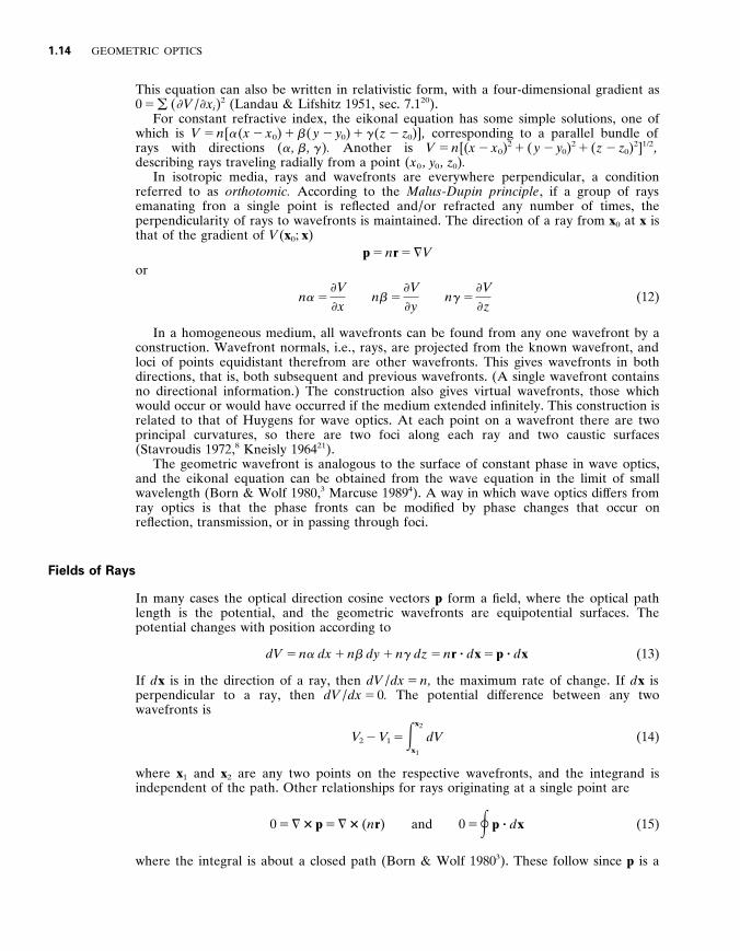
In many cases the optical direction cosine vectors p form a field , where the optical path length is the potential , and the geometric wavefronts are equipotential surfaces . The potential changes with position according to
dV 5 n a dx 1 n b dy 1 n g dz 5 n r ? d x 5 p ? d x (13)
If d x is in the direction of a ray , then dV / dx 5 n , the maximum rate of change . If d x is perpendicular to a ray , then dV / dx 5 0 . The potential dif ference between any two wavefronts is
V 2 2 V 1 5 E x 2
x 1
dV (14)
where x 1 and x 2 are any two points on the respective wavefronts , and the integrand is independent of the path . Other relationships for rays originating at a single point are
0 5 = 3 p 5 = 3 ( n r ) and 0 5 R p ? d x (15)
where the integral is about a closed path (Born & Wolf 1980 3 ) . These follow since p is a
GENERAL PRINCIPLES 1 .15
gradient , Eq . (13) . In regions where rays are folded onto themselves by refraction or reflections , p and V are not single-valued , so there is not a field .
1 . 4 CHARACTERISTIC FUNCTIONS
Introduction
Characteristic functions contain all the information about the path lengths between pairs of points , which may either be in a contiguous region or physically separated , e . g ., on the two sides of a lens . These functions were first considered by Hamilton (Hamilton 1931 2 2 ) , so their study is referred to as hamiltonian optics . They were rediscovered in somewhat dif ferent form by Bruns (Bruns 1895 , 2 3 Schwarzschild 1905 2 4 ) and referred to as eikonals , leading to a confusing set of names for the various functions . The subject is discussed in a number of books (Czapski-Eppenstein 1924 , 2 5 Steward 1928 , 2 6 Herzberger 1931 , 2 7 Synge 1937 , 2 8 Caratheodory 1937 , 2 9 Rayleigh 1908 , 3 0 Pegis 1961 , 3 1 Luneburg 1964 , 3 2 Brouwer and Walther 1967 , 3 3 Buchdahl 1970 , 3 4 Born & Wolf 1980 , 3 5 Herzberger 1958 3 6 ) .
Four parameters are required to specify a ray . For example , an input ray is defined in the z 5 0 plane by coordinates ( x , y ) and direction ( a , b ) . So four functions of four variables specify how an incident ray emerges from a system . In an output plane z 9 5 0 , the ray has coordinates x 9 5 x 9 ( x , y , a , b ) , y 9 5 y 9 ( x , y , a , b ) , and directions a 9 5 a 9 ( x , y , a , b ) , b 9 5 b 9 ( x , y , a , b ) . Because of Fermat’s principle , these four functions are not independent , and the geometrical optics properties of a system can be fully characterized by a single function (Luneburg 1964 , sec . 19 3 2 ) .
For any given system , there is a variety of characteristic functions related by Legendre transformations , with dif ferent combinations of spatial and angular variables (Buchdahl 1970 3 4 ) . The dif ferent functions are suited for dif ferent types of analysis . Mixed characteristic functions have both spatial and angular arguments . Those functions that are of most general use are discussed below . The others may be useful in special circum- stances . If the regions have constant refractive indices , the volumes over which the characteristic functions are defined can be extended virtually from physically accessible to inaccessible regions .
From any of its characteristic functions , all the properties of a system involving ray paths can be found , for example , ray positions , directions , and geometric wavefronts . An important use of characteristic functions is demonstrating general principles and fun- damental limitations . Much of this can be done by using the general properties , e . g ., symmetry under rotation . (Unfortunately , it is not always known how closely the impossible can be approached . )
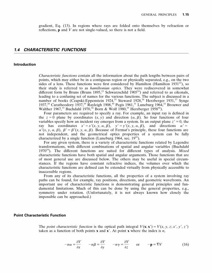
Point Characteristic Function
The point characteristic function is the optical path integral V ( x ; x 9 ) 5 V ( x , y , z ; x 9 , y 9 , z 9 ) taken as a function of both points x and x 9 . At point x where the index is n ,
2 n a 5 V
x 2 n b 5
V
y 2 n g 5
V
z or 2 p 5 = V (16)

1 .16 GEOMETRIC OPTICS
Similarly , at x 9 , where the index is n 9 ,
n 9 a 9 5 V x 9
n 9 b 9 5 V y 9
n 9 g 9 5 V z 9
or p 9 5 = 9 V (17)
It follows from the above equations and Eq . (4) that the point characteristic satisfies two conditions :
n 2 5 u = V u 2 and n 9 2 5 u = 9 V u 2 (18)
Therefore , the point characteristic is not an arbitrary function of six variables . The total dif ferential of V is
dV ( x ; x 9 ) 5 p 9 ? d x 9 2 p ? d x (19)
‘‘This expression can be said to contain all the basic laws of optics’’ (Herzberger 1958 3 6 ) .
Point Eikonal
If reference planes in object and image space are fixed , for which we use z 0 and z 9 0 , then the point eikonal is S ( x , y ; x 9 , y 9 ) 5 V ( x , y , z 0 ; x 9 , y 9 , z 9 0 ) . This is the optical path length between pairs of points on the two planes . The function is not useful if the planes are conjugate , since more than one ray through a pair of points can have the same path length . The function is arbitrary , except for the requirement (Herzberger 1936 3 8 ) that
2 S
x x 9
2 S
y y 9 2
2 S
x y 9
2 S
x 9 y ? 0 (20)
The partial derivatives of the point eikonal are
2 n a 5 S
x 2 n b 5
S
y and n 9 a 9 5
S
x 9 n 9 b 9 5
S
y 9 (21)
The relative merits of the point characteristic function and point eikonal have been debated . (Herzberger 1936 , 3 8 Herzberger 1937 , 3 9 Synge 1937 4 0 ) .
Angle Characteristic
The angle characteristic function T ( a , b ; a 9 , b 9 ) , also called the eikonal , is related to the point characteristic by
T ( a , b ; a 9 , b 9 ) 5 V ( x , y , z ; x 9 , y 9 , z 9 ) 1 n ( a x 1 b y 1 g z )
2 n 9 ( a 9 x 9 1 b 9 y 9 1 g 9 z 9 ) (22)
Here the input plane z and output plane z 9 are fixed and are implicit parameters of T .

GENERAL PRINCIPLES 1 .17
FIGURE 1 Geometrical interpretation of the angle characteristic function for constant object and image space indices . There is , in general , a single ray with directions ( a , b , g ) in object space and ( a 9 , b 9 , g 9 ) in image space . Point O is the coordinate origin in object space , and O 9 is that in image space . From the origins , perpendiculars to the ray are constructed , which intersect the ray at Q and Q 9 . The angle characteristic function T ( a , b ; a 9 , b 9 ) is the path length from Q to Q 9 .
This equation is really shorthand for a Legendre transformation to coordinates p x 5 V / x , etc . In principle , the expressions of Eq . (16) are used to solve for x and y in terms of a and b , and likewise Eq . (17) gives x 9 and y 9 in terms of a 9 and b 9 , so
T ( a , b ; a 9 , b 9 ) 5 V ( x ( a , b ) , y ( a , b ) , z ; x 9 ( a 9 , b 9 ) , y 9 ( a 9 , b 9 ) , z 9 )
1 n [ a x ( a , b ) 1 b y ( a , b ) 1 4 1 2 a 2 2 b 2 z ]
2 n 9 [ a 9 x 9 ( a 9 , b 9 ) 1 b 9 y 9 ( a 9 , b 9 ) 1 4 1 2 a 9 2 2 b 9 2 z 9 ] (23)
The angle characteristic is an arbitrary function of four variables that completely specify the directions of rays in two regions . This function is not useful if parallel incoming rays give rise to parallel outgoing rays , as is the case with afocal systems , since the relationship between incoming and outgoing directions is not unique . The partial derivatives of the angular characteristic function are
T a
5 n S x 2 a
g z D T
b 5 n S y 2
b
g z D (24)
T a 9
5 2 n 9 S x 9 2 a 9
g 9 z 9 D T
b 9 5 2 n 9 S y 9 2
b 9
g 9 z 9 D (25)
These expressions are simplified if the reference planes are taken to be z 5 0 and z 9 5 0 . The geometrical interpretation of T is that it is the path length between the intersection point of rays with perpendicular planes through the coordinate origins in the two spaces , as shown in Fig . 1 for the case of constant n and n 9 . If the indices are heterogeneous , the construction applies to the tangents to the rays . Of all the characteristic functions , T is most easily found for single surfaces and most easily concatenated for series of surfaces .
Point-Angle Characteristic
The point - angle characteristic function is a mixed function defined by
W ( x , y , z ; a 9 , b 9 ) 5 V ( x , y , z ; x 9 , y 9 , z 9 ) 2 n 9 ( a 9 x 9 1 b 9 y 9 1 g 9 z 9 )
5 T ( a , b ; a 9 , b 9 ) 2 n ( a x 1 b y 1 g z ) (26)
As with Eq . (22) , this equation is to be understood as shorthand for a Legendre transformation . The partial derivatives with respect to the spatial variables are related by
1 .18 GEOMETRIC OPTICS
equations like those of Eq . (16) , so n 2 5 u = W u 2 , and the derivatives with respect to the angular variables are like those of Eq . (25) . This function is useful for examining transverse ray aberrations for a given object point , since W / a 9 , W / b 9 give the intersection points ( x 9 , y 9 ) in plane z for rays originating at ( x , y ) in plane z .
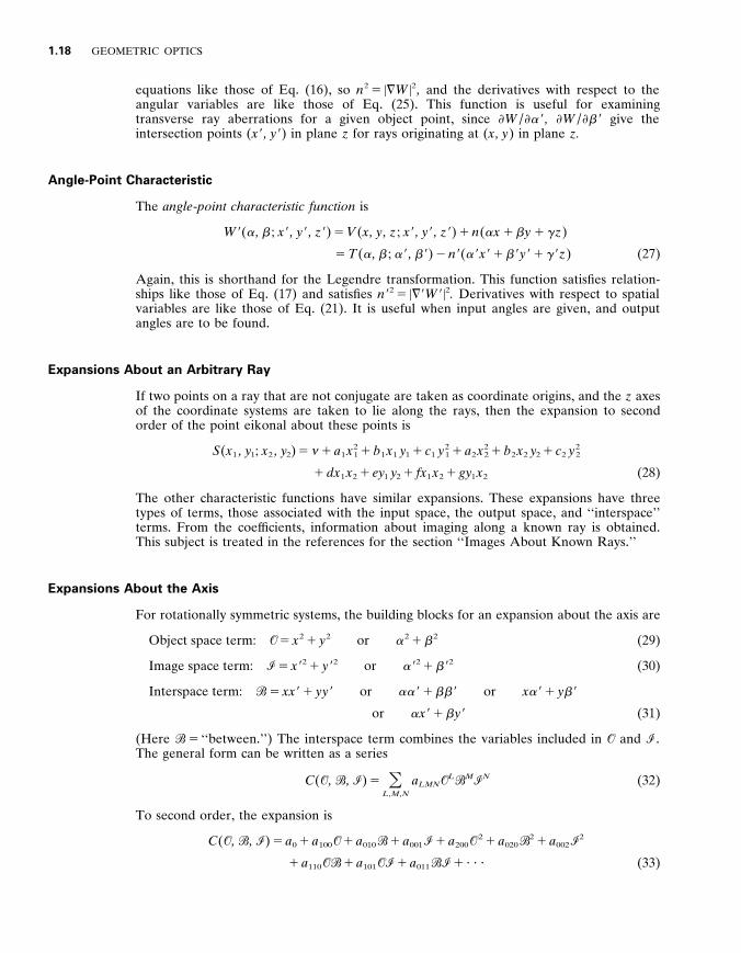
Angle-Point Characteristic
The angle - point characteristic function is
W 9 ( a , b ; x 9 , y 9 , z 9 ) 5 V ( x , y , z ; x 9 , y 9 , z 9 ) 1 n ( a x 1 b y 1 g z )
5 T ( a , b ; a 9 , b 9 ) 2 n 9 ( a 9 x 9 1 b 9 y 9 1 g 9 z ) (27)
Again , this is shorthand for the Legendre transformation . This function satisfies relation- ships like those of Eq . (17) and satisfies n 9 2 5 u = 9 W 9 u 2 . Derivatives with respect to spatial variables are like those of Eq . (21) . It is useful when input angles are given , and output angles are to be found .
Expansions About an Arbitrary Ray
If two points on a ray that are not conjugate are taken as coordinate origins , and the z axes of the coordinate systems are taken to lie along the rays , then the expansion to second order of the point eikonal about these points is
S ( x 1 , y 1 ; x 2 , y 2 ) 5 … 1 a 1 x 2 1 1 b 1 x 1 y 1 1 c 1 y 2
1 1 a 2 x 2 2 1 b 2 x 2 y 2 1 c 2 y 2
2
1 dx 1 x 2 1 ey 1 y 2 1 fx 1 x 2 1 gy 1 x 2 (28)
The other characteristic functions have similar expansions . These expansions have three types of terms , those associated with the input space , the output space , and ‘‘interspace’’ terms . From the coef ficients , information about imaging along a known ray is obtained . This subject is treated in the references for the section ‘‘Images About Known Rays . ’’
Expansions About the Axis
For rotationally symmetric systems , the building blocks for an expansion about the axis are
Object space term : 2 5 x 2 1 y 2 or a 2 1 b 2 (29)
Image space term : ( 5 x 9 2 1 y 9 2 or a 9 2 1 b 9 2 (30)
Interspace term : @ 5 xx 9 1 yy 9 or a a 9 1 b b 9 or x a 9 1 y b 9
or a x 9 1 b y 9 (31)
(Here @ 5 ‘‘between . ’’) The interspace term combines the variables included in 2 and ( . The general form can be written as a series
C ( 2 , @ , ( ) 5 O L ,M ,N
a L M N 2 L @ M ( N (32)
To second order , the expansion is
C ( 2 , @ , ( ) 5 a 0 1 a 1 0 0 2 1 a 0 1 0 @ 1 a 0 0 1 ( 1 a 2 0 0 2 2 1 a 0 2 0 @ 2 1 a 0 0 2 ( 2
1 a 1 1 0 2@ 1 a 1 0 1 2( 1 a 0 1 1 @( 1 ? ? ? (33)
GENERAL PRINCIPLES 1 .19
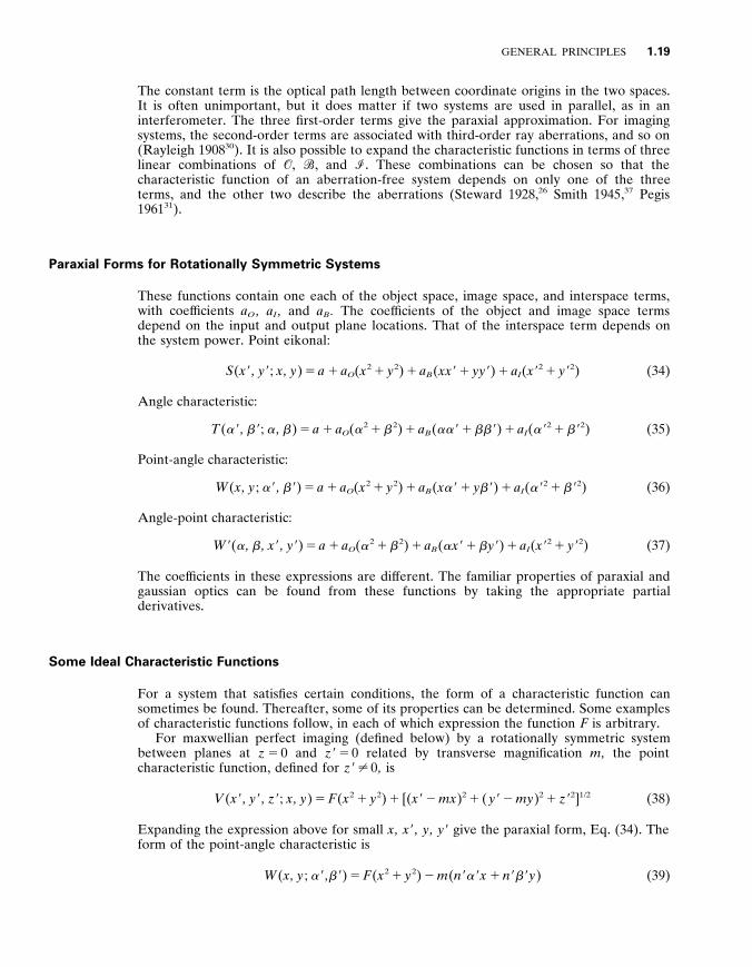
The constant term is the optical path length between coordinate origins in the two spaces . It is often unimportant , but it does matter if two systems are used in parallel , as in an interferometer . The three first-order terms give the paraxial approximation . For imaging systems , the second-order terms are associated with third-order ray aberrations , and so on (Rayleigh 1908 3 0 ) . It is also possible to expand the characteristic functions in terms of three linear combinations of 2 , @ , and ( . These combinations can be chosen so that the characteristic function of an aberration-free system depends on only one of the three terms , and the other two describe the aberrations (Steward 1928 , 2 6 Smith 1945 , 3 7 Pegis 1961 3 1 ) .
Paraxial Forms for Rotationally Symmetric Systems
These functions contain one each of the object space , image space , and interspace terms , with coef ficients a O , a I , and a B . The coef ficients of the object and image space terms depend on the input and output plane locations . That of the interspace term depends on the system power . Point eikonal :
S ( x 9 , y 9 ; x , y ) 5 a 1 a O ( x 2 1 y 2 ) 1 a B ( xx 9 1 yy 9 ) 1 a I ( x 9 2 1 y 9 2 ) (34)
Angle characteristic :
T ( a 9 , b 9 ; a , b ) 5 a 1 a O ( a 2 1 b 2 ) 1 a B ( a a 9 1 b b 9 ) 1 a I ( a 9 2 1 b 9 2 ) (35)
Point-angle characteristic :
W ( x , y ; a 9 , b 9 ) 5 a 1 a O ( x 2 1 y 2 ) 1 a B ( x a 9 1 y b 9 ) 1 a I ( a 9 2 1 b 9 2 ) (36)
Angle-point characteristic :
W 9 ( a , b , x 9 , y 9 ) 5 a 1 a O ( a 2 1 b 2 ) 1 a B ( a x 9 1 b y 9 ) 1 a I ( x 9 2 1 y 9 2 ) (37)
The coef ficients in these expressions are dif ferent . The familiar properties of paraxial and gaussian optics can be found from these functions by taking the appropriate partial derivatives .
Some Ideal Characteristic Functions
For a system that satisfies certain conditions , the form of a characteristic function can sometimes be found . Thereafter , some of its properties can be determined . Some examples of characteristic functions follow , in each of which expression the function F is arbitrary .
For maxwellian perfect imaging (defined below) by a rotationally symmetric system between planes at z 5 0 and z 9 5 0 related by transverse magnification m , the point characteristic function , defined for z 9 ? 0 , is
V ( x 9 , y 9 , z 9 ; x , y ) 5 F ( x 2 1 y 2 ) 1 [( x 9 2 mx ) 2 1 ( y 9 2 my ) 2 1 z 9 2 ] 1 / 2 (38)
Expanding the expression above for small x , x 9 , y , y 9 give the paraxial form , Eq . (34) . The form of the point-angle characteristic is
W ( x , y ; a 9 , b 9 ) 5 F ( x 2 1 y 2 ) 2 m ( n 9 a 9 x 1 n 9 b 9 y ) (39)

1 .20 GEOMETRIC OPTICS
The form of the angle-point characteristic is
W 9 ( a , b ; x 9 , y 9 ) 5 F ( x 9 2 1 y 9 2 ) 1 1 m
( n a x 9 1 n b y 9 ) (40)
The functions F are determined if the imaging is also stigmatic at one additional point , for example , at the center of the pupil (Steward 1928 , 2 6 T . Smith 1945 , 3 7 Buchdahl 1970 , 3 4
Velzel 1991 4 1 ) . The angular characteristic function has the form
T ( a , b ; a 9 , b 9 ) 5 F (( n a 2 mn 9 a 9 ) 2 1 ( n b 2 mn 9 b 9 ) 2 ) (41)
where F is any function . For a lens of power f that stigmatically images objects at infinity in a plane , and does so
in either direction ,
S ( x , y ; x 9 , y 9 ) 5 2 f ( xx 9 1 yy 9 ) and T ( a , b ; a 9 , b 9 ) 5 nn 9
f ( a a 9 1 b b 9 ) (42)
Partially dif ferentiating with respect to the appropriate variables shows that for such a system , the heights of point images in the rear focal plane are proportional to the sines of the incident angles , rather than the tangents .
1 . 5 RAYS IN HETEROGENEOUS MEDIA
Introduction
This section provides equations for describing and determining the curved ray paths in a heterogeneous or inhomogeneous medium , one whose refractive index varies with position . It is assumed here that n ( x ) and the other relevant functions are continuous and have continuous derivatives to whatever order is needed . Various aspects of this subject are discussed in a number of books and papers (Heath 1895 , 4 2 Herman 1900 , 4 3 Synge 1937 , 4 4 Luneburg 1964 , 4 5 Stavroudis 1972 , 4 6 Ghatak 1978 , 4 7 Born & Wolf 1980 , 4 8 Marcuse 1989 4 9 ) . This material is often discussed in the literature on gradient index lenses (Marchand 1973 , 5 0 Marchand 1978 , 5 1 Sharma , Kumar , & Ghatak 1982 , 5 2 Moore 1992 , 5 3
Moore 1994 5 4 ) and in discussions of microwave lenses (Brown 1953 , 5 5 Cornbleet 1976 , 5 6
Cornbleet 1983 , 5 7 Cornbleet 1984 5 8 ) .
Dif ferential Geometry of Space Curves
A curved ray path is a space curve , which can be described by a standard parametric description , x ( s ) 5 ( x ( s ) , y ( s ) , z ( s )) , where s is an arbitrary parameter (Blaschke 1945 , 5 9
Kreyszig 1991 , 6 0 Stoker 1969 , 6 1 Struik 1990 , 6 2 Stavroudis 1972 4 6 ) . Dif ferent parameters may be used according to the situation . The path length s along
the ray is sometimes used , as is the axial position z . Some equations change form according to the parameter , and those involving derivatives are simplest when the parameter is s . Derivatives with respect to the parameter are denoted by dots , so x Ù ( s ) 5 d x ( s ) / d s 5 ( x ~ ( s ) , y ~ ( s ) , z ~ ( s )) . A parameter other than s is a function of s , so d x ( s ) / ds 5 ( d x / d s )( d s / ds ) .
Associated with space curves are three mutually perpendicular unit vectors , the tangent

GENERAL PRINCIPLES 1 .21
vector t , the principal normal n , and the binormal b , as well as two scalars , the curvature and the torsion . The direction of a ray is that of its unit tangent y ector
t 5 x Ù ( s )
u x Ù ( s ) u 5 x Ù ( s ) 5 ( a , b , g ) (43)
The tangent vector t is the same as the direction vector r used elsewhere in this chapter . The rate of change of the tangent vector with respect to path length is
k n 5 t Ù ( s ) 5 x ̈ ( s ) 5 S d a
dx , d b
ds , d g
ds D (44)
The normal y ector is the unit vector in this direction
n 5 x ̈ ( s )
u x ̈ ( s ) u (45)
The vectors t and n define the osculating plane . The cur y ature k 5 u x ̈ ( s ) u is the rate of change of direction of t in the osculating plane .
k 2 5 u x Ù ( s ) 3 x ̈ ( s ) u 2
u x Ù ( s ) u 6 5 u x ̈ ( s ) u 2 5 S d a
ds D 2
1 S d b
ds D 2
1 S d g
ds D 2
(46)
The radius of curvature is r 5 1 / k . Perpendicular to the osculating plane is the unit binormal y ector
b 5 t 3 n 5 x Ù ( s ) 3 x ̈ ( s )
u x ̈ ( s ) u (47)
The torsion is the rate of change of the normal to the osculating plane
τ 5 b ( s ) ? d n ( s )
ds 5
( x Ù ( s ) 3 x ̈ ( s )) ? x & ( s ) u x Ù ( s ) 3 x ̈ ( s ) u 2
5 ( x Ù ( s ) 3 x ̈ ( s )) ? x & ( s )
u x ̈ ( s ) u 2 (48)
The quantity 1 / τ is the radius of torsion . For a plane curve , τ 5 0 and b is constant . The rates of change of t , n , and b are given by the Frenet equations :
t Ù ( s ) 5 k n n Ù ( s ) 5 2 k t 1 τ b b Ù ( s ) 5 2 τ n (49)
In some books , 1 / k and 1 / τ are used for what are denoted here by k and τ .
Dif ferential Geometry Equations Specific to Rays
From the general space curve equations above and the dif ferential equations below specific to rays , the following equations for rays are obtained . Note that n here is the refractive index , unrelated to n . The tangent and normal vectors are related by Eq . (59) , which can be written
= log n 5 k n 1 ( = log n ? t ) t (50)
The osculating plane always contains the vector = n . Taking the dot product with n in the above equation gives
k 5 log n
N 5 n ? = log n 5 b ? ( x Ù 3 = log n ) (51)

1 .22 GEOMETRIC OPTICS
The partial derivative / N is in the direction of the principal normal , so rays bend toward regions of higher refractive index . Other relations (Stavroudis 1972 4 6 ) are
n 5 r x Ù ( s ) 3 ( = log n 3 x Ù ( s )) (52)
b 5 r x Ù ( s ) 3 = log n and 0 5 b ? = n (53)
τ 5 ( x Ù ( s ) 3 = n ) ? = n ~
u = n 3 x Ù ( s ) u 2 (54)
Variational Integral
Written in terms of parameter s , the optical path length integral , Eq . (7) is
V 5 E n ds 5 E S n ds
d s D d s 5 E + d s (55)
The solution for ray paths involves the calculus of variations in a way analogous to that used in classical mechanics , where the time integral of the lagrangian + is an extremum (Goldstein 1980 6 3 ) . If + has no explicit dependence on s , the mechanical analogue to the optics case is that of no explicit time dependence .
Dif ferential Equations for Rays
General Dif ferential Equations . Because the optical path length integral is an extremum , the integrand + satisfies the Euler equations (Stavroudis 1972 4 6 ) . For an arbitrary coordinate system , with coordinates q 1 , q 2 , q 3 and the derivatives with respect to the parameter q ~ i 5 dq i / d s , the dif ferential equations for the path are
0 5 d
d s
+
q ~ i 2
+
q i 5
d d s
S n
q ~ i
ds d s
D 2
q i S n
ds d s
D i 5 1 , 2 , 3 (56)
Cartesian Coordinates with Unspecified Parameter . In cartesian coordinates ds / d s 5 ( x ~ 2 1 y ~ 2 1 z ~ 2 ) 1 / 2 , so the x equation is
0 5 d
d s S n
x ~ ds
d s D 2
ds
d s
n
x 5
d
d s F nx ~
( x ~ 2 1 y ~ 2 1 z ~ 2 ) 1 / 2 G 2 ( x ~ 2 1 y ~ 2 1 z ~ 2 ) 1 / 2 n
x (57)
Similar equations hold for y and z .
Cartesian Coordinates with Parameter s 5 s . With s 5 s , so ds / d s 5 1 , an expression , sometimes called the ray equation , is obtained (Synge 1937 2 8 ) .
= n 5 d
ds S n
d x ( s ) ds
D 5 n d 2 x ( s )
ds 2 1 dn ( x ( s ))
ds
d x ( s ) ds
(58)
Using dn / ds 5 = n ? x Ù , the ray equation can also be written
= n 5 n x ̈ 1 ( = n ? x Ù ) x Ù or = log n 5 x ̈ 1 ( = log n ? x Ù ) x Ù (59)
Only two of the component equations are independent , since u x Ù u 5 1 .
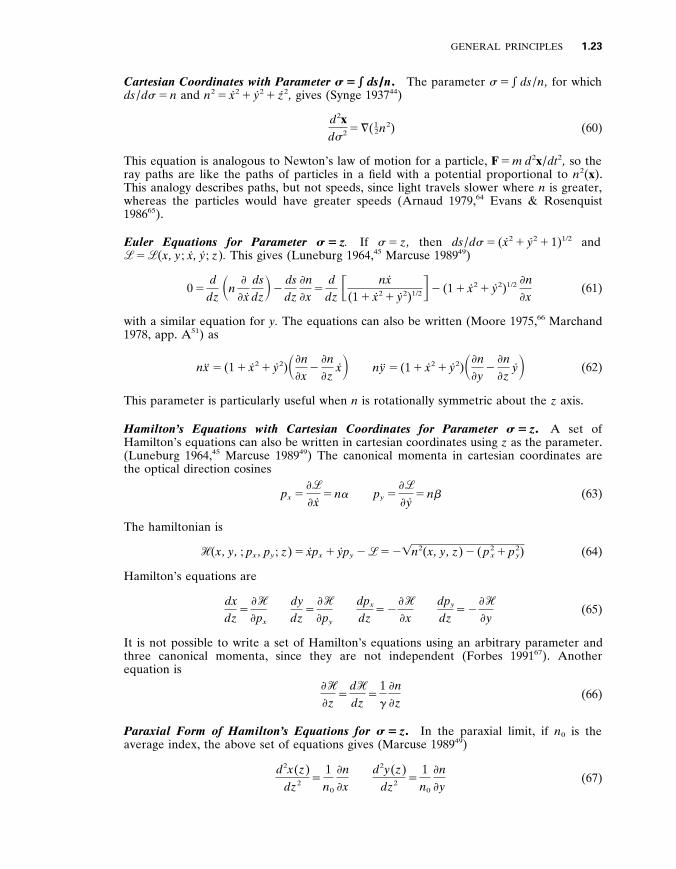
GENERAL PRINCIPLES 1 .23
Cartesian Coordinates with Parameter s 5 e e ds / n . The parameter s 5 e ds / n , for which ds / d s 5 n and n 2 5 x ~ 2 1 y ~ 2 1 z ~ 2 , gives (Synge 1937 4 4 )
d 2 x d s 2 5 = ( 1 – 2 n 2 ) (60)
This equation is analogous to Newton’s law of motion for a particle , F 5 m d 2 x / dt 2 , so the ray paths are like the paths of particles in a field with a potential proportional to n 2 ( x ) . This analogy describes paths , but not speeds , since light travels slower where n is greater , whereas the particles would have greater speeds (Arnaud 1979 , 6 4 Evans & Rosenquist 1986 6 5 ) .
Euler Equations for Parameter s 5 z . If s 5 z , then ds / d s 5 ( x ~ 2 1 y ~ 2 1 1) 1 / 2 and + 5 + ( x , y ; x ~ , y ~ ; z ) . This gives (Luneburg 1964 , 4 5 Marcuse 1989 4 9 )
0 5 d
dz S n
x ~ ds dz D 2
ds dz
n x
5 d
dz F nx ~
(1 1 x ~ 2 1 y ~ 2 ) 1 / 2 G 2 (1 1 x ~ 2 1 y ~ 2 ) 1 / 2 n x
(61)
with a similar equation for y . The equations can also be written (Moore 1975 , 6 6 Marchand 1978 , app . A 5 1 ) as
nx ̈ 5 (1 1 x ~ 2 1 y ~ 2 ) S n x
2 n z
x ~ D ny ̈ 5 (1 1 x ~ 2 1 y ~ 2 ) S n y
2 n z
y ~ D (62)
This parameter is particularly useful when n is rotationally symmetric about the z axis .
Hamilton’s Equations with Cartesian Coordinates for Parameter s 5 z . A set of Hamilton’s equations can also be written in cartesian coordinates using z as the parameter . (Luneburg 1964 , 4 5 Marcuse 1989 4 9 ) The canonical momenta in cartesian coordinates are the optical direction cosines
p x 5 +
x ~ 5 n a p y 5
+
y ~ 5 n b (63)
The hamiltonian is
* ( x , y , ; p x , p y ; z ) 5 x ~ p x 1 y ~ p y 2 + 5 2 4 n 2 ( x , y , z ) 2 ( p 2 x 1 p 2
y ) (64)
Hamilton’s equations are
dx dz
5 *
p x
dy dz
5 *
p y
dp x
dz 5 2
*
x dp y
dz 5 2
*
y (65)
It is not possible to write a set of Hamilton’s equations using an arbitrary parameter and three canonical momenta , since they are not independent (Forbes 1991 6 7 ) . Another equation is
*
z 5
d *
dz 5
1 g
n
z (66)
Paraxial Form of Hamilton’s Equations for s 5 z . In the paraxial limit , if n 0 is the average index , the above set of equations gives (Marcuse 1989 4 9 )
d 2 x ( z ) dz 2 5
1 n 0
n
x
d 2 y ( z ) dz 2 5
1 n 0
n
y (67)
1 .24 GEOMETRIC OPTICS
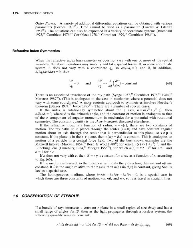
Other Forms . A variety of additional dif ferential equations can be obtained with various parameters (Forbes 1991 6 7 ) . Time cannot be used as a parameter (Landau & Lifshitz 1951 6 8 ) . The equations can also be expressed in a variety of coordinate systems (Buchdahl 1973 , 6 9 Cornbleet 1976 , 5 6 Cornbleet 1978 , 7 0 Cornbleet 1979 , 7 1 Cornbleet 1984 5 8 ) .
Refractive Index Symmetries
When the refractive index has symmetry or does not vary with one or more of the spatial variables , the above equations may simplify and take special forms . If , in some coordinate system , n does not vary with a coordinate q i , so n / q i 5 0 , and if , in addition , / q i ( ds / d s ) 5 0 , then
+
q i 5 0 and
+
q ~ 5 n
q ~ S ds
d s D 5 constant (68)
There is an associated invariance of the ray path (Synge 1937 , 4 4 Cornbleet 1976 , 5 6 1984 , 5 8
Marcuse 1989 4 9 ) . (This is analogous to the case in mechanics where a potential does not vary with some coordinate . ) A more esoteric approach to symmetries involves Noether’s theorem (Blaker 1974 , 7 2 Joyce 1975 7 3 ) . There are a number of special cases .
If the index is rotationally symmetric about the z axis , n 5 n ( x 2 1 y 2 , z ) , then + / f 5 0 , where f is the azimuth angle , and the constant of motion is analogous to that of the z component of angular momentum in mechanics for a potential with rotational symmetry . The constant quantity is the skew in y ariant , discussed elsewhere .
If the refractive index is a function of radius , n 5 n ( r ) , there are two constants of motion . The ray paths lie in planes through the center ( r 5 0) and have constant angular motion about an axis through the center that is perpendicular to this plane , so x 3 p is constant . If the plane is in the x - y plane , then n ( a y 2 b x ) is constant . This is analogous to motion of a particle in a central force field . Two of the best-known examples are the Maxwell fisheye (Maxwell 1854 , 7 4 Born & Wolf 1980 4 8 ) for which n ( r ) ~ (1 1 r 2 ) 2 1 , and the Luneburg lens (Luneburg 1964 , 4 5 Morgan 1958 7 5 ) , for which n ( r ) 5 4 2 2 r 2 for r # 1 and n 5 1 for r . 1 .
If n does not vary with z , then * 5 n g is constant for a ray as a function of z , according to Eq . (66) .
If the medium is layered , so the index varies in only the z direction , then n a and n b are constant . If θ is the angle relative to the z axis , then n ( z ) sin θ ( z ) is constant , giving Snell’s law as a special case .
The homogeneous medium , where n / x 5 n / y 5 n / z 5 0 , is a special case in which there are three constants of motion , n a , n b , and n g , so rays travel in straight lines .
1 . 6 CONSERVATION OF E ́ TENDUE
If a bundle of rays intersects a constant z plane in a small region of size dx dy and has a small range of angles d a d b , then as the light propagates through a lossless system , the following quantity remains constant :
n 2 dx dy d a d b 5 n 2 dA d a d b 5 n 2 dA cos θ d v 5 dx dy dp x dp y (69)

GENERAL PRINCIPLES 1 .25
Here dA 5 dx dy is the dif ferential area , d v is the solid angle , and θ is measured relative to the normal to the plane . The integral of this quantity
E n 2 dx dy d a d b 5 E n 2 dA d a d b 5 E n 2 dA cos θ d v 5 E dx dy dp x dp y (70)
is the e ́ tendue , and is also conserved . For lambertian radiation of radiance L e , the total power transferred is P 5 e L e n
2 d a d b dx dy . The e ́ tendue and related quantities are known by a variety of names (Steel 1974 7 6 ) , including generalized Lagrange in y ariant , luminosity , light - gathering power , light grasp , throughput , acceptance , optical extent , and area - solid - angle - product . The angle term is not actually a solid angle , but is weighted . It does approach a solid angle in the limit of small extent . In addition , the integrations can be over area , giving n 2 d a d b e dA , or over angle , giving n 2 dA e d a d b . A related quantity is the geometrical vector flux (Winston 1979 7 7 ) , with components ( e dp y dp z , e dp x dp z , e dp x dp y ) . In some cases these quantities include a brightness factor , and in others they are purely geometrical . The e ́ tendue is related to the information capacity of a system (Gabor 1961 7 8 ) .
As special case , if the initial and final planes are conjugate with transverse magnification m 5 dx 9 / dx 5 dy 9 / dy , then
n 2 d a d b 5 n 9 2 m 2 d a 9 d b 9 (71)
Consequently , the angular extents of the entrance and exit pupil in direction cosine coordinates are related by
n 2 E entrance pupil
d a d b 5 n 9 2 m 2 E exit pupil
d a 9 d b 9 (72)
See also the discussion of image irradiance in the section on apertures and pupils . This conservation law is general ; it does not depend on index homogeneity or on axial
symmetry . It can be proven in a variety of ways , one of which is with characteristic functions (Welford & Winston 1978 , 7 9 Welford 1986 , 8 0 Welford & Winston 1989 8 1 ) . Phase space arguments involving Liouville’s theorem can also be applied (di Francia 1950 , 8 2
Winston 1970 , 8 3 Jannson & Winston 1986 , 8 4 Marcuse 1989 8 5 ) . Another type of proof involves thermodynamics , using conservation of radiance (or brightness) or the principal of detailed balance (Clausius 1864 , 8 6 Clausius 1879 , 8 7 Helmholtz 1874 , 8 8 Liebes 1969 8 9 ) . Conversely , the thermodynamic principle can be proven from the geometric optics one (Nicodemus 1963 , 9 0 Boyd 1983 , 9 1 Klein 1986 9 2 ) . In the paraxial limit for systems of revolution the conservation of etendue between object and image planes is related to the two-ray paraxial invariant , Eq . (152) . Some historical aspects are discussed by Rayleigh (Rayleigh 1886 9 3 ) and Southall (Southall 1910 9 4 ) .
1 . 7 SKEW INVARIANT
In a rotationally symmetric system , whose indices may be constant or varying , a skew ray is one that does not lie in a plane containing the axis . The skewness of such a ray is
6 5 n ( a y 2 b x ) 5 n a y 2 n b x 5 p x y 2 p y x (73)
As a skew ray propagates through the system , this quantity , known as the skew in y ariant , does not change (T . Smith 1921 , 9 5 H . Hopkins 1947 , 9 6 Marshall 1952 , 9 7 Buchdahl 1954 , sec . 4 , 9 8 M . Herzberger 1958 , 9 9 Welford 1968 , 1 0 0 Stavroudis 1972 , p . 208 , 1 0 1 Welford 1974 , sec . 5 . 4 , 1 0 2 Welford 1986 , sec . 6 . 4 1 0 3 Welford & Winston 1989 , p . 228 1 0 4 ) . For a meridional ray ,

1 .26 GEOMETRIC OPTICS
one lying in a plane containing the axis , 6 5 0 . The skewness can be written in vector form as
6 5 a ? ( x 3 p ) (74)
where a is a unit vector along the axis , x is the position on a ray , and p is the optical cosine and vector at that position .
This invariance is analogous to the conservation of the axial component of angular momentum in a cylindrical force field , and it can be proven in several ways . One is by performing the rotation operations on a , b , x , and y (as discussed in the section on heterogeneous media) . Another is by means of characteristic functions . It can also be demonstrated that 6 is not changed by refraction or reflection by surfaces with radial gradients . The invariance holds also for dif fractive optics that are figures of rotation .
A special case of the invariant relates the intersection points of a skew ray with a given meridian . If a ray with directions ( a , b ) in a space of index n intersects the x 5 0 meridian with height y , then at another intersection with this meridian in a space with index n 9 , its height y 9 and direction cosine a 9 are related by
n a y 5 n 9 a 9 y 9 (75)
The points where rays intersect the same meridian are known as diapoints and the ratio y 9 / y as the diamagnification (Herzberger 1958 9 9 ) .
1 . 8 REFRACTION AND REFLECTION AT INTERFACES BETWEEN HOMOGENEOUS MEDIA
Introduction
The initial ray direction is specified by the unit vector r 5 ( a , b , g ) . After refraction or reflection the direction is r 9 5 ( a 9 , b 9 , g 9 ) . At the point where the ray intersects the surface , its normal has direction S 5 ( L , M , N ) .
The angle of incidence I is the angle between a ray and the surface normal at the intersection point . This angle and the corresponding outgoing angle I 9 are given by
(76) u cos I u 5 u r ? S u 5 u a L 1 b M 1 g N u
u cos I 9 u 5 u r 9 ? S u 5 u a 9 L 1 b 9 M 1 g 9 N u In addition
u sin I u 5 u r 3 S u u sin I 9 u 5 u r 9 3 S u (77)
The signs of these expressions depend on which way the surface normal vector is directed . The surface normal and the ray direction define the plane of incidence , which is perpendicular to the vector cross product S 3 r 5 ( M g 2 N b , N a 2 L g , L b 2 M a ) . After refraction or reflection , the outgoing ray is in the same plane . This symmetry is related to the fact that optical path length is an extremum .
The laws of reflection and refraction can be derived from Fermat’s principle , as is done in many books . At a planar interface , the reflection and refraction directions are derived from Maxwell’s equations using the boundary conditions . For scalar waves at a plane interface , the directions are related to the fact that the number of oscillation cycles is the same for incident and outgoing waves .

GENERAL PRINCIPLES 1 .27
Refraction
At an interface between two homogeneous and isotropic media , described by indices n and n 9 , the incidence angle I and the outgoing angle I 9 are related by Snell ’ s law (Magie 1963 1 0 5 ) :
n 9 sin I 9 5 n sin I (78)
If sin I 9 . 1 , there is total internal reflection . Another relationship is
n 9 cos I 9 5 4 n 9 2 2 n 2 sin 2 I 5 4 n 9 2 2 n 2 2 n 2 cos 2 I (79)
Snell’s law can be expressed in a number of ways , one of which is
n [ r 1 ( r ? S ) S ] 5 n 9 [ r 9 1 ( r 9 ? S ) S ] (80)
Taking the cross product of both sides with S gives another form
n 9 ( S 3 r 9 ) 5 n ( S 3 r ) (81)
A quantity that appears frequently in geometrical optics (but which has no common name or symbol) is
G 5 n 9 cos I 9 2 n cos I (82)
It can be written several ways
G 5 ( n r 2 n 9 r 9 ) ? S 5 2 n cos I 1 4 n 9 2 2 n 2 sin 2 I 5 2 n cos I 1 4 n 9 2 2 n 2 1 n 2 cos 2 I (83)
In terms of G , Snell’s law is n 9 r 9 5 n r 1 G S (84)
or n 9 a 9 5 n a 1 L G n 9 b 9 5 n b 1 M G n 9 g 9 5 n g 1 N G (85)
The outgoing direction is expressed explicitly as a function of incident direction by
n 9 r 9 5 n r 1 S [ n r ? S 2 4 n 9 2 2 n 2 1 ( n r ? S ) 2 ] (86)
If the surface normal is in the z direction , the equations simplify to
n 9 a 9 5 n a n 9 b 9 5 n b n 9 g 9 5 4 n 9 2 2 n 2 1 n 2 g 2 (87)
If b 5 0 , this reduces to n 9 a 9 5 n a , the familiar form of Snell’s law , written with direction cosines , with n 9 g 9 5 ( n 9 2 2 n 2 a 2 ) 1 / 2 , corresponding to Eq . (79) . Another relation is
n 9 a 9 2 n a
L 5
n 9 b 9 2 n b
M 5
n 9 g 9 2 n g
N 5 G (88)
All of the above expressions can be formally simplified by using p 5 n r and p 9 5 n 9 r 9 . For a succession of refractions by parallel surfaces ,
n 1 sin I 1 5 n 2 sin I 2 5 n 3 sin I 3 5 ? ? ? (89)
so the angles within any two media are related by their indices alone , regardless of the intervening layers . Refractive indices vary with wavelength , so the angles of refraction do likewise .
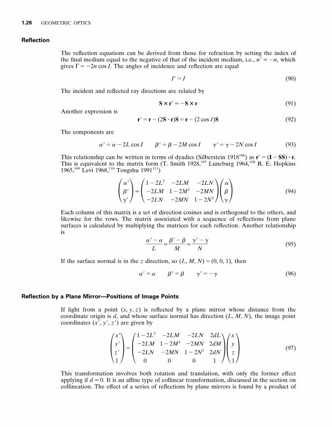
1 .28 GEOMETRIC OPTICS
Reflection
The reflection equations can be derived from those for refraction by setting the index of the final medium equal to the negative of that of the incident medium , i . e ., n 9 5 2 n , which gives G 5 2 2 n cos I . The angles of incidence and reflection are equal
I 9 5 I (90)
The incident and reflected ray directions are related by
S 3 r 9 5 2 S 3 r (91) Another expression is
r 9 5 r 2 (2 S ? r ) S 5 r 2 (2 cos I ) S (92)
The components are
a 9 5 a 2 2 L cos I b 9 5 b 2 2 M cos I g 9 5 g 2 2 N cos I (93)
This relationship can be written in terms of dyadics (Silberstein 1918 1 0 6 ) as r 9 5 ( I 2 SS ) ? r . This is equivalent to the matrix form (T . Smith 1928 , 1 0 7 Luneburg 1964 , 1 0 8 R . E . Hopkins 1965 , 1 0 9 Levi 1968 , 1 1 0 Tongshu 1991 1 1 1 )
1 a 9
b 9
g 9 2 5 1 1 2 2 L 2
2 2 LM
2 2 LN
2 2 LM 1 2 2 M 2
2 2 MN
2 2 LN 2 2 MN
1 2 2 N 2 2 1 a
b
g 2 (94)
Each column of this matrix is a set of direction cosines and is orthogonal to the others , and likewise for the rows . The matrix associated with a sequence of reflections from plane surfaces is calculated by multiplying the matrices for each reflection . Another relationship is
a 9 2 a
L 5
b 9 2 b
M 5
g 9 2 g
N (95)
If the surface normal is in the z direction , so ( L , M , N ) 5 (0 , 0 , 1) , then
a 9 5 a b 9 5 b g 9 5 2 g (96)
Reflection by a Plane Mirror—Positions of Image Points
If light from a point ( x , y , z ) is reflected by a plane mirror whose distance from the coordinate origin is d , and whose surface normal has direction ( L , M , N ) , the image point coordinates ( x 9 , y 9 , z 9 ) are given by
1 x 9
y 9
z 9
1 2 5 1
1 2 2 L 2
2 2 LM
2 2 LN
0
2 2 LM
1 2 2 M 2
2 2 MN
0
2 2 LN
2 2 MN
1 2 2 N 2
0
2 dL
2 dM
2 dN
1 2 1
x
y
z
1 2 (97)
This transformation involves both rotation and translation , with only the former ef fect applying if d 5 0 . It is an af fine type of collinear transformation , discussed in the section on collineation . The ef fect of a series of reflections by plane mirrors is found by a product of

GENERAL PRINCIPLES 1 .29
such matrices . The transformation can also be formulated in terms of quaternions (Wagner 1951 , 1 1 2 Levi 1968 , p . 367 1 1 0 ) .
Dif fractive Elements
The changes in directions produced by gratings or dif fractive elements can be handled in an ad hoc geometrical way (Spencer & Murty 1962 , 1 1 3 di Francia 1950 1 1 4 )
n 9 r 9 G 3 S 5 n r 3 S 1 G l
p q (98)
Here l is the vacuum wavelength , p is the grating period , q is a unit vector tangent to the surface and parallel to the rulings , and G is the dif fraction order . Equations (81) and (91) are special cases of this equation for the 0th order .
1 . 9 IMAGING
Introduction
Image formation is the principal use of lenses . Moreover , lenses form images even if this is not their intended purpose . This section provides definitions , and discusses basic concepts and limitations . The purposes of the geometric analysis of imaging include the following : (1) discovering the nominal relationship between an object and its image , principally the size , shape , and location of the image , which is usually done with paraxial optics ; (2) determining the deviations from the nominal image , i . e ., the aberrations ; (3) estimating image irradiance ; (4) understanding fundamental limitations—what is inherently possible and impossible ; (5) supplying information for dif fraction calculations , usually optical path lengths .
Images and Types of Images
A definition of image (Webster 1934 1 1 5 ) is : ‘‘The optical counterpart of an object produced by a lens , mirror , or other optical system . It is a geometrical system made up of foci corresponding to the parts of the object . ’’ The point-by-point correspondence is the key , since a given object can have a variety of dif ferent images .
Image irradiance can be found only approximately from geometric optics , the degree of accuracy of the predictions varying from case to case . In many instances wave optics is required , and for objects that are not self-luminous , an analysis involving partial coherence is also needed .
The term image is used in a variety of ways , so clarification is useful . The light from an object produces a three-dimensional distribution in image space . The aerial image is the distribution on a mathematical surface , often that of best focus , the locus of points of the images of object points . An aerial image is never the final goal ; ultimately , the light is to be captured . The recei y ing surface (NS) is that on which the light falls , the distribution of which there can be called the recei y ed image (NS) . This distinction is important in considerations of defocus , which is a relationship , not an absolute . The record thereby produced is the recorded image (NS) . The recorded image varies with the position of the receiving surface , which is usually intended to correspond with the aerial image surface . In this section , ‘‘image’’ means aerial image , unless otherwise stated .

1 .30 GEOMETRIC OPTICS
Object Space and Image Space
The object is said to exist in object space ; the image , in image space . Each space is infinite , with a physically accessible region called real , and an inaccessible region , referred to as y irtual . The two spaces may overlap physically , as with reflective systems . Corresponding quantities and locations associated with the object and image spaces are typically denoted by the same symbol , with a prime indicating image space . Positions are specified by a coordinate system ( x , y , z ) in object space and ( x 9 , y 9 , z 9 ) in image space . The refractive indices of the object and image spaces are n and n 9 .
Image of a Point
An object point is thought of as emitting rays in all directions , some of which are captured by the lens , whose internal action converges the rays , more or less , to an image point , the term ‘‘point’’ being used even if the ray convergence is imperfect . Object and image points are said to be conjugate . Since geometric optics is reversible , if A 9 is the image of A , then A is the image of A 9 .
Mapping Object Space to Image Space
If every point were imaged stigmatically , then the entire object space would be mapped into the image space according to a transformation
x 9 5 x 9 ( x , y , z ) y 9 5 y 9 ( x , y , z ) z 9 5 z 9 ( x , y , z ) (99)
The mapping is reciprocal , so the equations can be inverted . If n and n 9 are constant , then the mapping is a collinear transformation , discussed below .
Images of Extended Objects
An extended object can be thought of as a collection of points , a subset of the entire space , and its stigmatic image is the set of conjugate image points . A surface described by 0 5 F ( x , y , z ) has an image surface
0 5 F 9 ( x 9 , y 9 , z 9 ) 5 F ( x ( x 9 , y 9 , z 9 ) , y ( x 9 , y 9 , z 9 ) , z ( x 9 , y 9 , z 9 )) (100)
A curve described parametrically by x ( s ) 5 ( x ( s ) , y ( s ) , z ( s )) has an image curve
x 9 ( s ) 5 ( x 9 ( x ( s ) , y ( s ) , z ( s )) , y 9 ( x ( s ) , y ( s ) , z ( s )) , z 9 ( x ( s ) , y ( s ) , z ( s ))) (101)
Rotationally Symmetric Lenses
Rotationally symmetric lenses have an axis , which is a ray path (unless there is an obstruction) . All planes through the axis , the meridians or meridional planes , are planes with respect to which there is bilateral symmetry . An axial object point is conjugate to an axial image point . An axial image point is located with a single ray in addition to the axial one . Of f-axis object and image points are in the same meridian , and may be on the same or opposite sides of the axis . The object height is the distance of a point from the axis , and the

GENERAL PRINCIPLES 1 .31
image height is that for its image . It is possible to have rotational symmetry without bilateral symmetry , as in a system made of crystalline quartz (Buchdahl 1970 1 1 6 ) , but such systems are not discussed here . For stigmatic imaging by a lens rotationally symmetric about the z axis , Eq . (99) gives
x 9 5 x 9 ( x , z ) y 9 5 y 9 ( y , z ) z 9 5 z 9 ( z ) (102)
Planes Perpendicular to the Axis
The arrangement most often of interest is that of planar object and receiving surfaces , both perpendicular to the lens axis . When the terms object plane and image plane are used here without further elaboration , this is the meaning . (This arrangement is more common for manufactured systems with flat detectors , than for natural systems , for instance , eyes , with their curved retinas . )
Magnifications
The term magnification is used in a general way to denote the ratio of conjugate object and image dimensions , for example , heights , distances , areas , volumes , and angles . A single number is inadequate when object and image shapes are not geometrically similar . The term magnification implies an increase , but this is not the case in general .
Transverse Magnification
With object and image planes perpendicular to the axis , the relative scale factor of length is the trans y erse magnification or lateral magnification , denoted by m , and usually referred to simply as ‘‘the magnification . ’’ The transverse magnification is the ratio of image height to object height , m 5 h 9 / h . It can also be written in dif ferential form , e . g ., m 5 dx 9 / dx or m 5 D x 9 / D x . The transverse magnification is signed , and it can have any value from 2 ̀ to 1 ̀ . Areas in such planes are scaled by m 2 . A lens may contain plane mirrors that af fect the image parity or it may be accompanied by external plane mirrors that reorient images and change their parity , but these changes are independent of the magnification at which the lens works .
Longitudinal Magnification
Along the rotational axis , the longitudinal magnification , m L , also called axial magnification , is the ratio of image length to object length in the limit of small lengths , i . e ., m L 5 dz 9 / dz .
Visual Magnification
With visual instruments , the perceived size of the image depends on its angular subtense . Visual magnification is the ratio of the angular subtense of an image relative to that of the object viewed directly . Other terms are used for this quantity , including ‘‘magnification , ’’ ‘‘power , ’’ and ‘‘magnifying power . ’’ For objects whose positions can be controlled , there is arbitrariness in the subtense without the instrument , which is greatest when the object is located at the near-point of the observer . This distance varies from person to person , but for purposes of standardization the distance is taken to be 250 mm . For instruments that view distant objects there is no arbitrariness of subtense with direct viewing .
1 .32 GEOMETRIC OPTICS
Ideal Imaging and Disappointments in Imaging
Terms such as perfect imaging and ideal imaging are used in various ways . The ideal varies with the circumstances , and there are applications in which imaging is not the purpose , for instance , energy collection and Fourier transformation . The term desired imaging might be more appropriate in cases where that which is desired is fundamentally impossible . Some deviations from what is desired are called aberrations , whether their avoidance is possible or not . Any ideal that can be approximated must agree in its paraxial limit ideal with what a lens actually does in its paraxial limit .
Maxwellian Ideal for Single-Plane Imaging
The most common meaning of perfect imaging is that elucidated by Maxwell (Maxwell 1858 1 1 7 ) , and referred to here as maxwellian ideal or maxwellian perfection . This ideal is fundamentally possible . The three conditions for such imaging of points in a plane perpendicular to the lens axis are : (1) Each point is imaged stigmatically . (2) The images of all the points in a plane lie on a plane that is likewise perpendicular to the axis , so the field is flat , or free from field curvature . (3) The ratio of image heights to object heights is the same for all points in the plane . That is , transverse magnification is constant , or there is no distortion .
The Volume Imaging Ideal
A more demanding ideal is that points everywhere in regions of constant index be imaged stigmatically and that the imaging of every plane be flat and free from distortion . For planes perpendicular to the lens axis , such imaging is described mathematically by the collinear transformation , discussed below . It is inherently impossible for a lens to function in this way , but the mathematical apparatus of collineation is useful in obtaining approximate results .
Paraxial , First-Order , and Gaussian Optics
The terms ‘‘paraxial , ’’ ‘‘first order , ’’ and ‘‘gaussian’’ are often used interchangeably , and their consideration is merged with that of collineation . The distinction is often not made , probably because these descriptions agree in result , although dif fering in approach . One of the few discussions is that of Southall (Southall 1910 1 1 8 ) . A paraxial analysis has to do with the limiting case in which the distances of rays from the axis approach zero , as do the angles of the rays relative to the axis . The term first order refers to the associated mathematical approximation in which the positions and directions of such rays are computed with terms to the first order only in height and angle . Gaussian refers to certain results of the paraxial optics , where lenses are black boxes whose properties are summarized by the existence and locations of cardinal points . In the limit of small heights and angles , the equations of collineation are identical to those of paraxial optics . Each of these is discussed in greater detail below .
Fundamental Limitations
There are fundamental geometrical limitations on optical systems , relating to the fact that a given ray passes through many points and a given point lies on many rays . So the images of points on the same line or plane , or on dif ferent planes , are not independent . A set of rays intersecting at several points in object space cannot be made to satisfy arbitrary

GENERAL PRINCIPLES 1 .33
requirements in image space . Such limitations are best studied by the methods of hamiltonian optics .
Stigmatic Imaging
If all rays from an object point converge precisely to an image point , the imaging of this point is said to be stigmatic . The optical path lengths of all rays between two such points is identical . A stigmatic image point is located by the intersection of any two rays that pass through the points . An absolute instrument is one which images all points stigmatically (Born & Wolf 1980 1 1 9 ) . For such imaging
n d x 5 n 9 d x 9 n d y 5 n 9 d y 9 n d z 5 n 9 d z 9 (103)
where conjugate length elements are d x and d x 9 , d y and d y 9 , d z and d z 9 .
Path Lengths and Conjugate Points
All the rays from an object point to its stigmatic image point have the same optical path length . For focal lenses , the paths lengths for dif ferent pairs of conjugate points in a plane perpendicular to the axis are dif ferent , except for points on circles centered on the axis . For afocal lenses path lengths are nominally the same for all points in planes perpendicular to the axis . For afocal lenses with transverse magnification Ú n / n 9 , path lengths can be the same for all points . In general , the path lengths between dif ferent points on an object and image surface are equal only if the shape of the image surface is that of a wavefront that has propagated from a wavefront whose shape is that of the object surface .
The Cosine Condition
The cosine condition relates object space and image space ray angles , if the imaging is stigmatic over some area (T . Smith 1922 , 1 2 0 Steward 1928 , 1 2 1 Buchdahl 1970 1 1 6 ) . Let the x - y plane lie in the object surface and the x 9 - y 9 plane in the conjugate surface (Fig . 2) . Two
FIGURE 2 The cosine condition . A small area in object space about the origin in the x - y plane is imaged to the region around the origin of the x 9 - y 9 plane in image space . A pair of rays from the origin with direction cosines ( a 1 , b 1 ) and ( a 2 , b 2 ) arrive with ( a 9 1 , b 9 1 ) and ( a 9 2 , b 9 2 ) . The direction cosines and the transverse magnification in the planes are related by Eq . (104) .

1 .34 GEOMETRIC OPTICS
rays leaving a point in the object region have direction cosines ( a 1 , b 1 ) and ( a 2 , b 2 ) , and the rays on the image side have ( a 9 1 , b 9 1 ) and ( a 9 2 , b 9 2 ) . If the imaging is stigmatic , with local transverse magnification m on the surface , then
m 5 n ( a 1 2 a 2 ) n 9 ( a 9 1 2 a 9 2 )
5 n ( b 1 2 b 2 ) n 9 ( b 9 1 2 b 9 2 )
(104)
In the limit as a 1 5 a 2 and b 1 5 b 2 , the cosine condition gives
m 5 n d a
n 9 d a 9 5
n d b
n 9 d b 9 (105)
This condition also holds in the more general case of isoplanatic imaging , where there is aberration that is locally constant across the region in question (Welford 1976 , 1 2 2 Welford 1986 , sec . 94 1 2 3 ) .
The Abbe Sine Condition
The sine condition or Abbe sine condition (Abbe 1879 , 1 2 4 Born & Wolf 1980 1 1 9 ) is a special case of the cosine condition for object and image planes perpendicular to the axis in regions about the axis . For a plane with transverse magnification m , let θ be the angle relative to the axis made by a ray from an axial object point , and θ 9 be that in image space . If the lens is free of coma
m 5 n sin θ
n 9 sin θ 9 5
n a
n 9 a 9 5
n b
n 9 b 9 (106)
for all θ and θ 9 . There are signs associated with θ and θ 9 , so that m . 0 if they have the same sign , and m , 0 if the signs are opposite . This equation is sometimes written with m replaced by the ratio of paraxial angles . There is sometimes the implication that θ and θ 9 refer only to the extreme angles passing through the lens , when in fact the sine condition dictates that the ratio of the sines is the constant for all angles . For an object at infinity , the sine condition is
sin θ 9 5 2 y f 9
or n 9 b 9 5 2 y f (107)
where y is the height of a ray parallel to the axis , f is the power of the lens , and f 9 is the rear focal length . These relationships hold to a good approximation in most lenses , since small deviations are associated with large aberrations . A deviation from this relationship is called of fense against the sine condition , and is associated with coma (Conrady 1992 , 1 2 5 H . Hopkins 1946 , 1 2 6 T . Smith 1948 , 1 2 7 H . Hopkins 1950 , 1 2 8 Welford 1986 1 2 3 ) . The sine condition does not apply where there are discontinuities in ray behavior , for example , in devices like Fresnel lenses , or to dif fraction-based devices like zone plates .
The Herschel Condition
The Herschel condition is a relationship that holds if the imaging is stigmatic for nearby points along the axis (Herschel 1821 , 1 2 9 H . Hopkins 1946 , 1 3 0 Born & Wolf 1980 1 1 9 ) . The two equivalent relations are
m 5 n sin ( 1 – 2 θ )
n 9 sin ( 1 – 2 θ 9 ) and m L 5
n sin 2 ( 1 – 2 θ ) n 9 sin 2 ( 1 – 2 θ 9 )
5 n (1 2 g )
n 9 (1 2 g 9 ) (108)

GENERAL PRINCIPLES 1 .35
The Herschel condition is inconsistent with the sine condition unless m Ú n / n 9 . So , in general , stigmatic imaging in one plane precludes that in others .
Sine and Herschel Conditions for Afocal Systems
For afocal systems the sine condition and Herschel condition are identical . For rays entering parallel to the axis at y and leaving at y 9 they are
m 5 y 9
y (109)
That is , the ratio of incoming and outgoing heights is independent of the incoming height . (H . Hopkins , 1 2 8 Chap . III ‘‘The Sine Condition and Herschel’s Condition . ’’)
Stigmatic Imaging Possibilities
For object and image spaces with constant refractive indices , stigmatic imaging is only possible for the entire spaces for afocal lenses with identical transverse and longitudinal magnifications m 5 Ú n / n 9 and u m L u 5 u m u . Such lenses re-create not only the intersection points , but the wavefronts , since the corresponding optical path lengths are the same in both spaces , Eq . (103) . For other lenses with constant object and image space indices , the maxwellian ideal can be met for only a single surface . In addition , a single point elsewhere can be imaged stigmatically (T . Smith 1948 , 1 2 7 Velzel 1991 1 3 1 ) . Nonplanar surfaces can be imaged stigmatically , a well-known example being the imaging of spherical surfaces by a spherical refracting surface , for a particular magnification (Born & Wolf 1980 , sec . 4 . 2 . 3 1 1 9 ) . For systems with spherical symmetry , it is possible that two nonplanar surfaces be stigmatically imaged (T . Smith 1927 1 3 2 ) . In addition , various systems with heterogeneous indices can image stigmatically over a volume .
1 . 1 0 DESCRIPTION OF SYSTEMS OF REVOLUTION
Introduction
This section is concerned with the optical description of lens and mirror systems that are figures of revolution . 133–145 From a mechanical viewpoint , optical systems are comprised of lenses and mirrors . From the point of view of the light , the system is regions of media with dif ferent indices , separated by interfaces of various shapes . This section is limited to homogeneous isotropic media . It is further restricted to reflecting and refracting surfaces that are nominally smooth , and to surfaces that are figures of revolution arranged so their axes are collinear , so the entire system is a figure of revolution about the lens axis . (The often-used term ‘‘optical axis’’ is also used in crystallography . Moreover , the axis is often mechanical as well as ‘‘optical . ’’) The lens axis is the z axis of an orthogonal coordinate system , with the x - y plane perpendicular . The distance from a point to the axis is r 5 4 x 2 1 y 2 . Along the axis , the positive direction is from left to right .
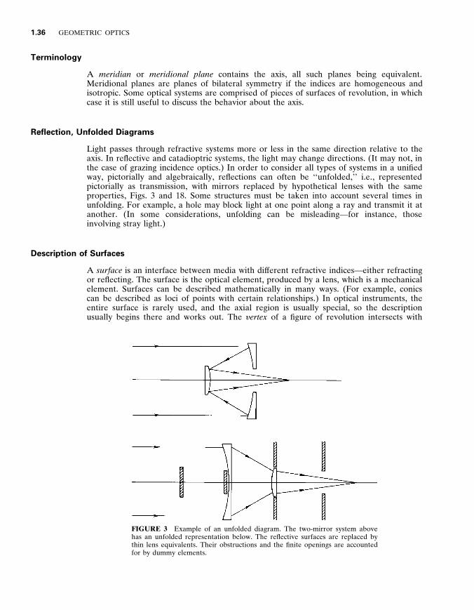
1 .36 GEOMETRIC OPTICS
Terminology
A meridian or meridional plane contains the axis , all such planes being equivalent . Meridional planes are planes of bilateral symmetry if the indices are homogeneous and isotropic . Some optical systems are comprised of pieces of surfaces of revolution , in which case it is still useful to discuss the behavior about the axis .
Reflection , Unfolded Diagrams
Light passes through refractive systems more or less in the same direction relative to the axis . In reflective and catadioptric systems , the light may change directions . (It may not , in the case of grazing incidence optics . ) In order to consider all types of systems in a unified way , pictorially and algebraically , reflections can often be ‘‘unfolded , ’’ i . e ., represented pictorially as transmission , with mirrors replaced by hypothetical lenses with the same properties , Figs . 3 and 18 . Some structures must be taken into account several times in unfolding . For example , a hole may block light at one point along a ray and transmit it at another . (In some considerations , unfolding can be misleading—for instance , those involving stray light . )
Description of Surfaces
A surface is an interface between media with dif ferent refractive indices—either refracting or reflecting . The surface is the optical element , produced by a lens , which is a mechanical element . Surfaces can be described mathematically in many ways . (For example , conics can be described as loci of points with certain relationships . ) In optical instruments , the entire surface is rarely used , and the axial region is usually special , so the description usually begins there and works out . The y ertex of a figure of revolution intersects with
FIGURE 3 Example of an unfolded diagram . The two-mirror system above has an unfolded representation below . The reflective surfaces are replaced by thin lens equivalents . Their obstructions and the finite openings are accounted for by dummy elements .
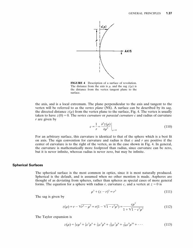
GENERAL PRINCIPLES 1 .37
FIGURE 4 Description of a surface of revolution . The distance from the axis is r , and the sag z ( r ) is the distance from the vertex tangent plane to the surface .
the axis , and is a local extremum . The plane perpendicular to the axis and tangent to the vertex will be referred to as the y ertex plane (NS) . A surface can be described by its sag , the directed distance z ( r ) from the vertex plane to the surface , Fig . 4 . The vertex is usually taken to have z (0) 5 0 . The y ertex cur y ature or paraxial cur y ature c and radius of curvature r are given by
c 5 1 r
5 2 z ( r )
r 2 U r 5 0
(110)
For an arbitrary surface , this curvature is identical to that of the sphere which is a best fit on axis . The sign convention for curvature and radius is that c and r are positive if the center of curvature is to the right of the vertex , as in the case shown in Fig . 4 . In general , the curvature is mathematically more foolproof than radius , since curvature can be zero , but it is never infinite , whereas radius is never zero , but may be infinite .
Spherical Surfaces
The spherical surface is the most common in optics , since it is most naturally produced . Spherical is the default , and is assumed when no other mention is made . Aspheres are thought of as deviating from spheres , rather than spheres as special cases of more general forms . The equation for a sphere with radius r , curvature c , and a vertex at z 5 0 is
r 2 1 ( z 2 r ) 2 5 r 2 (111) The sag is given by
z ( r ) 5 r 2 4 r 2 2 r 2 5 r (1 2 4 1 2 c 2 r 2 ) 5 c r 2
1 1 4 1 2 c 2 r 2 (112)
The Taylor expansion is
z ( r ) 5 1 – 2 c r 2 1 1 – 8 c 3 r 4 1 1 – 16 c 5 r 6 1 5 – 128 c 7 r 8 1 7 – 256 c 9 r 1 0 1 ? ? ? (113)

1 .38 GEOMETRIC OPTICS
At the point ( x , y , z ) on the surface of the sphere , the surface normal has direction cosines
( L , M , N ) 5 S x r
, y r
, z 2 r
r D 5 ( cx , cy , cz 2 1) (114)
Conics of Rotation
The general form of a conic of rotation about the z axis is
z ( r ) 5 r »
(1 2 4 1 2 » c 2 r 2 ) 5 c r 2
1 1 4 1 2 » c 2 r 2 (115)
The value of » determines the type of conic , as given in the table below . It is common in optics to use k , the conic parameter or conic constant , related by
k 5 » 2 1 or » 5 1 1 k (116)
Another parameter used to describe conics is the eccentricity e , used in the polar coordinate form for conics about their focus : r ( θ ) 5 a / (1 1 e cos θ ) where e 2 5 2 k . In the case of paraboloids , the first form of Eq . (115) breaks down . A cone can be approximated by a hyperbola with k 5 2 sec 2 θ , where θ is the cone half angle .
Conic Type and Value of Parameter
Parameter » k e
Oblate ellipsoid Sphere Prolate ellipsoid Paraboloid Hyperboloid
» . 1 » 5 1
0 , » , 1 » 5 0 » , 0
k . 0 k 5 0
2 1 , k , 0 k 5 2 1 k , 2 1
— 0
0 , e , 1 e 5 1 e . 1
The Taylor expansion for the sag is
z ( r ) 5 1 – 2 c r 2 1 1 – 8 » c 3 r 4 1 1 – 16 » 2 c 5 r 6 1 5 – 128 » 3 c 7 r 8 1 7 – 256 » 5 c 9 r 1 0 1 ? ? ? (117)
The surface normals are
( L , M , N ) 5 [1 2 2 c ( » 2 1) z 1 c 2 » ( » 2 1) z 2 ] 2 1 / 2 ( cx , cy , cz 2 1) (118)
The sagittal and tangential curvatures are
c s 5 c
[1 1 (1 2 » ) c 2 r 2 ] 1 / 2 c t 5 c
[1 1 (1 2 » ) c 2 r 2 ] 3 / 2 (119)
General Asphere of Revolution
For an arbitrary figure of revolution all of whose derivatives are continuous , the Taylor expansion is
z ( r ) 5 1 – 2 c r 2 1 q 4 r 4 1 q 6 r 6 1 ? ? ? (120)

GENERAL PRINCIPLES 1 .39
An asphere is often treated as a sphere that matches at the vertex and a deviation therefrom :
z ( r ) 5 z sphere ( r ) 1 a 4 r 4 1 a 6 r 6 1 ? ? ? (121)
Alternatively , nonconic aspheres can be treated as conics and a deviation therefrom :
z ( r ) 5 z conic ( r ) 1 b 4 r 4 1 b 6 r 6 1 ? ? ? (122)
The expansion coef ficients are dif ferent in each case . Additional information on the coef ficients is given by Malacara (Malacara 1992 1 4 4 ) and Brueggemann (Brueggemann 1968 1 3 5 ) . The sagittal and tangential curvatures are given in general by
c s 5 z ~ ( r )
r [1 1 z ~ ( r ) 2 ] 1 / 2 c t 5 z ̈ ( r )
[1 1 z ~ ( r ) 2 ] 3 / 2 (123)
Here z ~ ( r ) 5 dz ( r ) / d r and z ̈ ( r ) 5 d 2 z ( r ) / d r 2 .
1 . 1 1 TRACING RAYS IN CENTERED SYSTEMS OF SPHERICAL SURFACES
Introduction
Ray tracing is the process of calculating the paths of rays through optical systems . Two operations are involved , propagation from one surface to the next and refraction or reflection at the surfaces . Exact equations can be written for spherical surfaces and conics of revolution with homogeneous media (Spencer & Murty 1962 , 1 4 6 Welford 1974 , chap . 4 , 1 4 7 Kingslake 1978 , 1 4 8 Kinglake 1983 , 1 4 9 Slyusarev 1984 , 1 5 0 Klein & Furtak 1986 , sec . 3 . 1 , 1 5 1 Welford 1986 , chap . 4 , 1 5 2 W . J . Smith 1992 , chap . 10 1 5 3 ) . Conics are discussed by Welford (Welford 1986 , sec . 4 . 7 1 5 2 ) . For general aspheres , the intersection position is found by iterating (Nussbaum & Phillips , p . 95 , 1 5 4 W . J . Smith 1992 , sec . 10 . 5 1 5 3 ) . Nonsymmetric systems are discussed by Welford (Welford 1986 , chap . 5 1 5 2 ) .
Description and Classification of Rays in a Lens
For optical systems with rotational symmetry , rays are typically described in terms of the axial parameter z . A ray crosses each constant z plane at a point ( x , y ) with direction cosines ( a , b , g ) , where g is not independent . Thus a ray is described by ( x ( z ) , y ( z )) and ( a ( z ) , b ( z )) .
For systems that are figures of revolution , meridional rays are those lying in a meridional plane , a plane that includes the axis , and other rays are skew rays . The axial ray corresponds to the axis of revolution . Rays are also classified according to their proximity to the axis . Paraxial rays are those in the limit of having small angles and small distances from the axis . Nonparaxial rays are sometimes referred to as finite rays or real rays . Ray fans are groups of rays lying in a plane . A tangential fan lies in a meridian , and intersects

1 .40 GEOMETRIC OPTICS
at a tangential focus . A sagittal fan lies in a plane perpendicular to a meridian , and intersects at a sagittal focus .
Transfer
In propagating through a homogeneous medium , a ray originating at ( x 1 , y 1 , z 1 ) with directions ( a , b , g ) intersects a z 2 plane at
x 2 5 x 1 1 a
g ( z 2 2 z 1 ) and y 2 5 y 1 1
b
g ( z 2 2 z 1 ) (124)
Intersection Points
Let the intersection points of the ray with the vertex plane at z 5 0 be ( x 0 , y 0 , 0) , Fig . 5 . Define auxiliary functions
A ( x 0 , y 0 ; a , b ; c ) 5 g 2 c ( a x 0 1 b y 0 ) and B ( x 0 , y 0 , c ) 5 c 2 ( x 2 0 1 y 2
0 ) (125)
The distance D along the ray from this point to the surface is given by
cD 5 A 2 4 A 2 2 B 5 B
A 1 4 A 2 2 B (126)
The intersection point has the coordinates
x 5 x 0 1 a D y 5 y 0 1 b D z 5 g D (127)
The incidence angle I at the intersection point is given by
cos I 5 4 A 2 2 B (128) so
G 5 2 n 4 A 2 2 B 1 4 n 9 2 2 n 2 1 n 2 ( A 2 2 B ) (129)
Mathematically , double intersection points are possible , so they must be checked for . If
FIGURE 5 Intersection points . A ray with direc- tion cosines ( a , b , g ) intersects the vertex tangent plane at ( x 0 , y 0 , 0) and the optical surface at ( x , y , z ) . The distance between these points is D , given by Eq . (126) .
GENERAL PRINCIPLES 1 .41
the ray misses the surface , then A 2 , B . If there is total internal reflection , the second square root in Eq . (129) is imaginary .
Refraction and Reflection by Spherical Surfaces
Rays refract or reflect at surfaces with reference to the local normal at the intersection point . The surface normal given by Eq . (114) is substituted in the general form for refraction , Eq . (85) , to give
n 9 a 9 5 n a 2 G cx n 9 b 9 5 n b 2 G cy n 9 g 9 5 ny 2 G (1 2 cz ) (130)
For reflection , the above equations are used , with n 9 5 2 n , so G 5 2 n cos I 5 2 n 4 A 2 2 B .
Meridianal Rays
The meridian is customarily taken to be that for which x 5 0 , so the direction cosines are (0 , b , g ) . Let U be the angle between the axis and the ray , so b 5 sin U and g 5 cos U . The transfer equation , Eq . (124) becomes
y 2 5 y 1 1 tan U ( z 2 2 z 1 ) (131)
The second equation of Eq . (130) can be written
n 9 sin U 9 2 n sin U 5 2 cy ( n 9 cos I 9 2 n cos I ) (132)
If the directed distance from the vertex to the intersection point of the incident ray with the axis is l , the outgoing angle is
U 9 5 U 1 arcsin [( lc 2 1) sin U ] 2 arcsin F n n 9
( lc 2 1) sin U G (133)
The directed distance l 9 from the vertex to the axial intersection of the refracted ray is given by
cl 9 5 1 1 ( cl 2 1) n n 9
sin U sin U 9
(134)
For reflection , setting n 9 5 2 n gives
U 9 5 U 1 2 arcsin [( lc 2 1) sin U ] (135)
1 . 1 2 PARAXIAL OPTICS OF SYSTEMS OF REVOLUTION
Introduction
The term paraxial is used in dif ferent ways . In one , paraxial rays are those whose distances from the axis and whose angles relative to the axis are small . This leaves questions of how small is small enough and how this varies from system to system . The other interpretation of the term , which is used here , is that paraxial rays represent a limiting case in which the
1 .42 GEOMETRIC OPTICS
distances from the axis and angles relative to the axis vanish . Paraxial optics then describes the behavior of systems in this limit . The ray-tracing equations in the paraxial limit are linear in angle and in distance from the axis , hence the term first - order optics , which is often considered equivalent to paraxial . (There are no 0th-order terms since the expansion is taken about the axis , so a ray with an initial height and angle of zero , i . e ., a ray along the axis , has the same outgoing height and angle . ) The linearity of the paraxial equations makes them simple and understandable , as well as expressible in matrix form . Paraxial ray tracing is discussed to some extent by almost every book that treats geometrical optics .
Paraxial ray tracing is done to determine the gaussian properties of lenses , to locate image positions and magnifications , and to locate pupils and determine their sizes . Another use of paraxial ray tracing , not discussed here , is the computation of third-order aberrations (W . Smith 1992 1 5 5 ) .
Paraxial imaging is perfect in the sense that it agrees with the Maxwell ideal and with that of collineation . Point images everywhere are stigmatic , fields are flat , and there is no distortion . Aberration is often thought of as the dif ference between the behavior of finite rays and that of paraxial rays . If this approach is taken , then in the process of lens design , finite rays are made to agree , insofar as possible , with the paraxial ones , which cannot be similarly changed . In the paraxial limit , surfaces are described by their vertex curvatures , so conics , aspheres , and spheres are indistinguishable , the dif ference being in the fourth power and above . Consequently , aberrations can be altered by changing the surface asphericity without changing paraxial properties . A paraxial treatment can be done even if a system is missing the axial region , as in the case with central obstructions and of f-axis sections of figures of revolution .
This section is concerned with systems of mirrors and lenses with rotational symmetry and homogeneous refractive indices . In this case , it suf fices to work in a single meridian . Generalizations are found in the sections in this chapter on images about known rays and rays in heterogeneous media . Other generalizations involve expansions about given rays in systems that are not rotationally symmetric .
The Paraxial Limit
The lens axis is the z axis , and rays in the x 5 0 meridian are considered . Ray heights are y , and angles relative to the axis are u . In the paraxial limit , the quantities u , tan u , and sin u 5 b are indistinguishable . The z -direction cosine is g 5 cos u . 1 . Since the ray angles and heights are small , incidence angles are likewise , so i . sin i , cos I . 1 , cos I 9 . 1 , and G 5 n 9 cos I 9 2 n cos I . n 9 2 n .
Transfer
In traversing a distance t between two planes , the height of a meridional ray changes from y to y 9 according to Eq . (124) , y 9 5 y 1 t b / g . In the paraxial limit , this equation becomes
y 9 5 y 1 tu (136)
If a ray travels from one curved surface to the next , the distance t equals the vertex separation to first order , since the correction for the surface sag is of second order in height and angle . This term is given above in Eq . (127) .

GENERAL PRINCIPLES 1 .43
Refraction
The paraxial form of Snell’s law , Eq . (78) , is
n 9 i 9 5 ni (137)
Reflection
The law of reflection is the same for paraxial as for finite rays ,
i 9 5 2 i (138)
Angle of Incidence at a Surface
A ray with an angle u , which intersects a surface of curvature c at height y , makes an angle i with the local surface normal of the surface given by
i 5 u 1 yc (139)
This equation is easily remembered from two special cases . When y 5 0 , the intersection is at the vertex , so i 5 u . When u 5 2 cy , the ray is directed through the center of curvature , so i 5 0 .
Refraction at a Surface
The above equation combined with that for Snell’s law gives
n 9 u 9 5 nu 2 yc ( n 9 2 n ) (140)
This equation can also be obtained from the exact equation , n 9 b 9 5 n b 2 G cy , Eq . (125) . In the paraxial limit , G 5 n 9 2 n , and the intersection height y is that in the vertex plane .
Reflection at a Surface
The relationship between incident and outgoing angles at a reflecting surface is found by combining Eqs . (138) and (139) , to be
u 9 5 2 u 2 2 cy (141)
Refraction and Reflection United—Surface Power
Reflection and refraction can be treated the same way mathematically by thinking of reflection as refraction with n 9 5 2 n , in which case Eq . (140) gives Eq . (141) . A reflecting surface can be represented graphically as a thin convex-plano or concave-plano thin lens with index 2 n , where n is the index of the medium , Fig . 18 . For both refraction and reflection ,
n 9 u 9 5 nu 2 y f (142) where the surface power f is
f 5 c ( n 9 2 n ) (143)
If the surface is approached from the opposite direction , then n and n 9 are switched , as is the sign of c , so f is the same in both directions . Thus f is a scalar property of the interface , which can be positive , negative , or zero . The power is zero if n 9 5 n or c 5 0 . If n 9 5 n , the surface is ‘‘invisible , ’’ and the rays are not bent . If c 5 0 , the rays are bent . For a planar refracting surface n 9 u 9 5 nu , and a planar reflecting surface gives u 9 5 2 u .
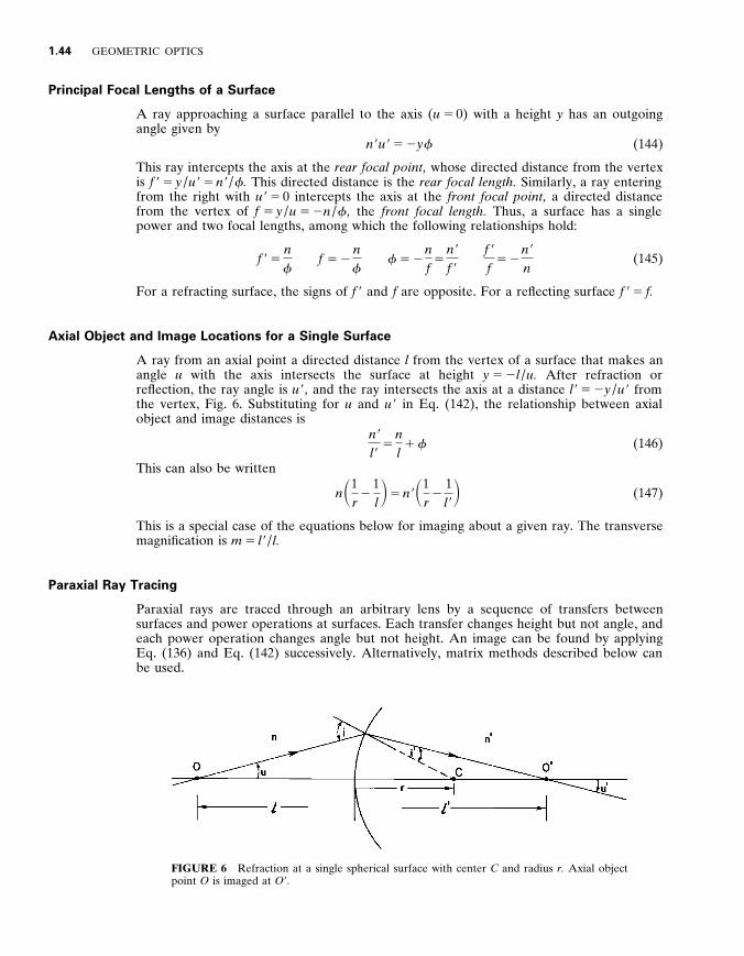
1 .44 GEOMETRIC OPTICS
Principal Focal Lengths of a Surface
A ray approaching a surface parallel to the axis ( u 5 0) with a height y has an outgoing angle given by
n 9 u 9 5 2 y f (144)
This ray intercepts the axis at the rear focal point , whose directed distance from the vertex is f 9 5 y / u 9 5 n 9 / f . This directed distance is the rear focal length . Similarly , a ray entering from the right with u 9 5 0 intercepts the axis at the front focal point , a directed distance from the vertex of f 5 y / u 5 2 n / f , the front focal length . Thus , a surface has a single power and two focal lengths , among which the following relationships hold :
f 9 5 n f
f 5 2 n f
f 5 2 n f
5 n 9
f 9
f 9
f 5 2
n 9
n (145)
For a refracting surface , the signs of f 9 and f are opposite . For a reflecting surface f 9 5 f .
Axial Object and Image Locations for a Single Surface
A ray from an axial point a directed distance l from the vertex of a surface that makes an angle u with the axis intersects the surface at height y 5 2 l / u . After refraction or reflection , the ray angle is u 9 , and the ray intersects the axis at a distance l 9 5 2 y / u 9 from the vertex , Fig . 6 . Substituting for u and u 9 in Eq . (142) , the relationship between axial object and image distances is
n 9
l 9 5
n l
1 f (146)
This can also be written
n S 1 r
2 1 l D 5 n 9 S 1
r 2
1 l 9 D (147)
This is a special case of the equations below for imaging about a given ray . The transverse magnification is m 5 l 9 / l .
Paraxial Ray Tracing
Paraxial rays are traced through an arbitrary lens by a sequence of transfers between surfaces and power operations at surfaces . Each transfer changes height but not angle , and each power operation changes angle but not height . An image can be found by applying Eq . (136) and Eq . (142) successively . Alternatively , matrix methods described below can be used .
FIGURE 6 Refraction at a single spherical surface with center C and radius r . Axial object point O is imaged at O 9 .
GENERAL PRINCIPLES 1 .45
Linearity of Paraxial Optics
For both the transfer and power operations , the outgoing heights and angles depend linearly on the incoming heights and angles . So a system described by a sequence of such operations is also linear . Therefore , a ray that enters with height y and angle u leaves with y 9 ( y , u ) and u 9 ( y , u ) given by
y 9 5 S y 9
y D y 1 S y 9
u D u and u 9 5 S u 9
y D y 1 S u 9
u D u (148)
These equations can also be thought of as the first terms of Taylor expansions of exact expressions for y 9 ( y , u ) and u 9 ( y , u ) . These partial derivatives depend on the structure of the system , and they can be determined by tracing two rays through the system . The partial derivatives , other than u 9 / y , also depend on the axial locations of the input and output surfaces . The changes with respect to these locations are treated easily by matrix methods .
The Two-Ray Paraxial Invariant
The various rays that pass through a lens are not acted upon independently , so there are several invariants that involve groups of rays . Consider two meridional paraxial rays that pass through a lens . At a given plane , where the medium has an index n , one ray has height y 1 and angle u 1 , and the other has y 2 and u 2 . The quantity
L 5 ny 1 u 2 2 ny 2 u 1 5 n ( y 1 u 2 2 y 2 u 1 ) (149)
which we refer to as the paraxial in y ariant (NS) , is unchanged as the rays pass through the system . Applying Eq . (136) and Eq . (142) to the above expression shows that this quantity does not change upon transfer or upon refraction and reflection . The invariant is also related to the general skew invariant , Eq . (73) , since a paraxial skew ray can be decomposed into two meridional rays .
Another version of the invariance relationship is as follows . Two objects with heights y 1 and y 2 are separated axially by d 1 2 . If their image heights are y 9 1 and y 9 2 , and the image separation is d 9 1 2 , then
n y 1 y 2
d 1 2 5 n 9
y 9 1 y 9 2
d 9 1 2 (150)
An additional version of the invariance relationship is
S y 9
y D S u 9
u D 2 S y 9
u D S u 9
y D 5
n n 9
(151)
where the partial derivatives , Eq . (148) , describe the action of any system . The invariant applies regardless of the system . Thus , for example , if the lens changes ,
as with a zoom system , so that both of the outgoing rays change , their invariant remains . The invariant arises from basic physical principles that are manifested in a variety of ways , for example , as conservation of brightness and Liouville’s theorem , discussed above in the section on conservation of etendue . This invariance shows that there are fundamental limits on what optical systems can do . Given the paraxial heights and angles of two input rays , only three of the four output heights and angles can be chosen arbitrarily . Likewise , only three of the four partial derivatives above can be freely chosen . The invariant is not useful if it vanishes identically . This occurs if the two rays are scaled versions of one another , which happens if both u 1 5 0 and u 2 5 0 for some z , or if both rays pass through the same axial object point , in which case y 1 5 0 and y 2 5 0 . The invariant also vanishes if one of the rays lies along the axis , so that y 1 5 0 and u 1 5 0 .
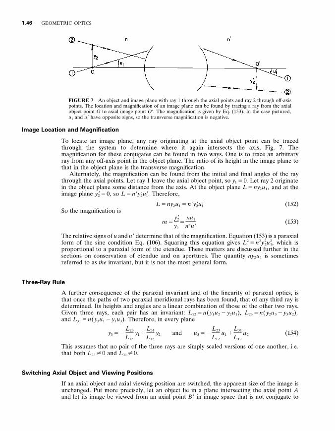
1 .46 GEOMETRIC OPTICS
FIGURE 7 An object and image plane with ray 1 through the axial points and ray 2 through of f-axis points . The location and magnification of an image plane can be found by tracing a ray from the axial object point O to axial image point O 9 . The magnification is given by Eq . (153) . In the case pictured , u 1 and u 9 1 have opposite signs , so the transverse magnification is negative .
Image Location and Magnification
To locate an image plane , any ray originating at the axial object point can be traced through the system to determine where it again intersects the axis , Fig . 7 . The magnification for these conjugates can be found in two ways . One is to trace an arbitrary ray from any of f-axis point in the object plane . The ratio of its height in the image plane to that in the object plane is the transverse magnification .
Alternately , the magnification can be found from the initial and final angles of the ray through the axial points . Let ray 1 leave the axial object point , so y 1 5 0 . Let ray 2 originate in the object plane some distance from the axis . At the object plane L 5 ny 2 u 1 , and at the image plane y 9 2 5 0 , so L 5 n 9 y 9 2 u 9 1 . Therefore ,
L 5 ny 2 u 1 5 n 9 y 9 2 u 9 1 (152) So the magnification is
m 5 y 9 2
y 2 5
nu 1
n 9 u 9 1 (153)
The relative signs of u and u 9 determine that of the magnification . Equation (153) is a paraxial form of the sine condition Eq . (106) . Squaring this equation gives L 2 5 n 2 y 2
2 u 2 1 , which is
proportional to a paraxial form of the etendue . These matters are discussed further in the sections on conservation of etendue and on apertures . The quantity ny 2 u 1 is sometimes referred to as the invariant , but it is not the most general form .
Three-Ray Rule
A further consequence of the paraxial invariant and of the linearity of paraxial optics , is that once the paths of two paraxial meridional rays has been found , that of any third ray is determined . Its heights and angles are a linear combination of those of the other two rays . Given three rays , each pair has an invariant : L 1 2 5 n ( y 1 u 2 2 y 2 u 1 ) , L 2 3 5 n ( y 2 u 3 2 y 3 u 2 ) , and L 3 1 5 n ( y 3 u 1 2 y 1 u 3 ) . Therefore , in every plane
y 3 5 2 L 2 3
L 1 2 y 1 1
L 3 1
L 1 2 y 2 and u 3 5 2
L 2 3
L 1 2 u 1 1
L 3 1
L 1 2 u 2 (154)
This assumes that no pair of the three rays are simply scaled versions of one another , i . e . that both L 2 3 ? 0 and L 3 1 ? 0 .
Switching Axial Object and Viewing Positions
If an axial object and axial viewing position are switched , the apparent size of the image is unchanged . Put more precisely , let an object lie in a plane intersecting the axial point A and let its image be viewed from an axial point B 9 in image space that is not conjugate to
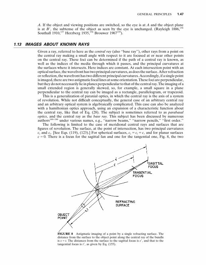
GENERAL PRINCIPLES 1 .47
A . If the object and viewing positions are switched , so the eye is at A and the object plane is at B 9 , the subtense of the object as seen by the eye is unchanged . (Rayleigh 1886 , 1 5 6
Southall 1910 , 1 5 7 Herzberg 1935 , 1 5 8 Brouwer 1967 1 5 9 ) .
1 . 1 3 IMAGES ABOUT KNOWN RAYS
Given a ray , referred to here as the central ray (also ‘‘base ray’’) , other rays from a point on the central ray making a small angle with respect to it are focused at or near other points on the central ray . These foci can be determined if the path of a central ray is known , as well as the indices of the media through which it passes , and the principal curvatures at the surfaces where it intersects . Here indices are constant . At each intersection point with an optical surface , the wavefront has two principal curvatures , as does the surface . After refraction or reflection , the wavefront has two dif ferent principal curvatures . Accordingly , if a single point is imaged , there are two astigmatic focal lines at some orientation . These foci are perpendicular , but they do not necessarily lie in planes perpendicular to that of the central ray . The imaging of a small extended region is generally skewed , so , for example , a small square in a plane perpendicular to the central ray can be imaged as a rectangle , parallelogram , or trapezoid .
This is a generalization of paraxial optics , in which the central ray is the axis of a system of revolution . While not dif ficult conceptually , the general case of an arbitrary central ray and an arbitrary optical system is algebraically complicated . This case can also be analyzed with a hamiltonian optics approach , using an expansion of a characteristic function about the central ray , like that of Eq . (28) . The subject is sometimes referred to as parabasal optics , and the central ray as the base ray . This subject has been discussed by numerous authors 160–186 under various names , e . g ., ‘‘narrow beams , ’’ ‘‘narrow pencils , ’’ ‘‘first order . ’’
The following is limited to the case of meridional central rays and surfaces that are figures of revolution . The surface , at the point of intersection , has two principal curvatures c s and c t . [See Eqs . (119) , (123) . ] For spherical surfaces , c s 5 c t 5 c , and for planar surfaces c 5 0 . There is a focus for the sagittal fan and one for the tangential one , Fig . 8 , the two
FIGURE 8 Astigmatic imaging of a point by a single refracting surface . The distance from the surface to the object point along the central ray of the bundle is s 5 t . The distances from the surface to the sagittal focus is s 9 , and that to the tangential focus is t 9 , as given by Eq . (155) .

1 .48 GEOMETRIC OPTICS
foci coinciding if the imaging is stigmatic . After one or more surfaces are encountered , the separated foci are the sources for subsequent imaging . Let s and t be the directed distances from the intersection point of the central ray and the surface to the object point , and s 9 and t 9 be the distances from intersection point to the foci . The separation u s 9 2 t 9 u is known as the astigmatic dif ference .
For refraction n 9
s 9 5
n
s 1 c s G and
n 9 cos 2 I 9
t 9 5
n cos 2 I
t 1 c t G (155)
where G 5 n 9 cos I 9 2 n cos I , Eq . (82) . The sagittal equation is simpler , providing a mnemonic for remembering which equation is which : ‘‘S’’ 5 sagittal 5 simpler . If the surface is spherical , and the ray fan makes an arbitrary angle of c with the meridian , then (H . Hopkins 1950 1 7 5 )
n 9
d 9 (1 2 cos 2 c sin 2 I 9 ) 5
n d
(1 2 cos 2 c sin 2 I ) 1 c G (156)
where d and d 9 are the distances along the central ray from the surface to the object and image points . For normal incidence at a spherical surface G 5 n 9 2 n , so both equations become
n 9
d 9 5
n d
1 c ( n 9 2 n ) (157)
This also applies to surfaces of revolution if the central ray lies along the axis . This equation is identical to the paraxial equation , Eq . (146) .
The corresponding relations for reflection are obtained by setting n 9 5 2 n and I 9 5 I in the refraction equations , giving
1 s 9
5 2 1 s
1 2 c s cos I and 1 t 9
5 2 1 t
1 2 c t
cos I (158)
For stigmatic imaging between the foci of reflective conics , s 5 t is the distance from one focus to a point on the surface , and s 9 5 t 9 is that from the surface to the other focus . Therefore , c t 5 c s cos 2 I . The reflection analogue to Eq . (156) , for a spherical surface is
1 d 9
5 2 1 d
1 2 c cos I
1 2 cos 2 c sin 2 I (159)
These equations are known by several names , including Coddington ’ s equations , Young ’ s astigmatic formulae , and the s - and t - trace formulae .
1 . 1 4 GAUSSIAN LENS PROPERTIES
Introduction
The meaning of the term gaussian optics is not universally agreed upon , and it is often taken to be indistinguishable from paraxial optics or first-order optics , as well as collineation . Here the term is considered to apply to those aspects of paraxial optics discovered by Gauss (Gauss 1840 1 8 7 ) , who recognized that all rotationally symmetric systems of lens elements can be described paraxially by certain system properties . In particular , lenses can be treated as black boxes described by two axial length parameters and the locations of special points , called cardinal points , also called Gauss points . Once a lens is so characterized , knowledge of its actual makeup is unnecessary for many purposes , and repeated ray traces need not be performed . For example , given the object location , the image location and magnification are determined from the gaussian parameters . From the

GENERAL PRINCIPLES 1 .49
gaussian description of two or more lenses , that of a coaxial combination can be found . Another consequence of Gauss’s discovery is that there is an infinity of specific embodiments for any external prescription .
The lenses considered in this section are figures of revolution with uniform object space and image space indices n and n 9 . All quantities discussed in this section are paraxial , so the prefix ‘‘paraxial’’ is not repeated . For the purposes of this section , no distinction is made between real and virtual rays . Those in each space are considered to extend infinitely , and intersection points may be either accessible or inaccessible . The quantities used in this section are found in Table 1 .
Power , Focal Lenses , and Afocal Lenses
A paraxial ray entering a lens parallel to the axis height y leaves with some angle u 9 , Fig . 9 . Likewise , a ray entering from the opposite side with height y 9 leaves with angle u . The power of the lens is defined by
f 5 2 n 9 u 9
y 5 n
u y 9
(160)
The outgoing ray can have any angle , and the power can be positive , negative , or zero . If u 9 5 0 , then f 5 0 and the lens is afocal or telescopic . Lenses for which f ? 0 are referred to here as focal , although the term ‘‘nonafocal’’ is more common . Afocal lenses are fundamentally dif ferent from focal ones , and are treated separately below . Power is the same in both directions , i . e . whether the ray enters from left to right or from right to left . The lens in Fig . 9 has f . 0 , and that in Fig . 10 has f , 0 . Diagrams such as Fig . 11 show the location of the principal focal point , but not the sign of the power ; two rays enter and two leave , but there is no indication of which is which . (Note that some negative lenses have accessible rear focal points . ) Another expression for power involves two rays at arbitrary angles and heights . If two incident rays have ( y 1 , u 1 ) and ( y 2 , u 2 ) , and a nonzero invariant L 5 n ( y 1 u 2 2 y 2 u 1 ) , and the outgoing ray angles are u 9 1 and u 9 2 , then
f 5 2 nn 9
L ( u 9 1 u 2 2 u 9 2 u 1 ) (161)
Focal Lenses
Focal lenses are those for which f ? 0 . Their cardinal points are the principal focal points , the principal points , and the nodal points . These points may be located anywhere on axis relative to the physical lens system . If they are inside a lens , then the intersection points referred to below are virtual . The cardinal points are pairs consisting of a member in object space and one in image space . The one in object space is often referred to as front , and the one in image space as rear , but this terminology may be misleading , since the points can be any sequence along the axis .
Principal Focal Points . Rays entering a lens parallel to its axis cross the axis at the principal focal points or focal points . Rays parallel to the axis in object space intersect the axis at the rear focal point F 9 in image space and those parallel in image space intersect at the front focal point F in object space , Fig . 9 . The principal focal planes or focal planes are the planes perpendicular to the axis at the focal points . The terms focal point and focal plane are often used to refer to the images of any point or plane . In this chapter , image point is used for other points where rays are focused and image plane for other planes .
Principal Planes . The principal planes are the conjugate planes for which the transverse

1 .50 GEOMETRIC OPTICS
TABLE 1 Gaussian Notation and Definitions
By convention , in the diagrams the object space is to the left of the lens , image space is to the right , and rays go left to right . Object space quantities are unprimed , and image space quantities are primed , and quantities or positions that correspond in some way have same symbol , primed and unprimed . This correspondence can have several forms , e . g ., the same type of thing or conjugate . The term front refers to object space , or left side , and rear to image space , or right side . A ‘‘front’’ entity may actually be behind a ‘‘rear’’ one . For example , a negative singlet has its object space focal point behind lens .
Scalars
n and n 9 object and image space refractive indices f power m transverse magnification m N nodal point magnification 5 n / n 9 m L longitudinal magnification m a angular magnification u and u 9 paraxial ray angles (the positive direction is counterclockwise from the axis) y and y 9 paraxial ray heights y P paraxial ray height at the principal planes 5 y 9 P
Axial points
Cardinal points : Focal points F and F 9 , not conjugate Principal points P and P 9 , conjugate m 5 1 1 Nodal points N and N 9 , conjugate m N 5 n / n 9
Other points : Axial object and image points O and O 9 , conjugate Arbitrary object and image points A and A 9 , B and B 9 Vertices V and V 9 , not conjugate , in general
Directed axial distances
These distances here are between axial points and are directed . Their signs are positive if from left to right and vice versa . Types of distances : entirely in object or image space , between spaces Principal focal lengths : f 5 PF and f 9 5 P 9 F 9 Principal points to object and image axial points : l 5 PO and l 9 5 P 9 O 9 Front and rear focal points to object and image axial points : z 5 FO and z 9 5 F 9 O 9
Relations : l 5 f 1 z and l 9 5 f 9 1 z 9 Arbitrary point to conjugate object and image points : d 5 AO and d 9 5 A 9 O 9
Distances between object space and image space points involve distances within both spaces , as well as a distance between the spaces , e . g ., PP 9 , FF 9 , VV 9 , and OO 9 . The distances between spaces depend on the particular structure of the lens . They can be found by paraxial ray tracing .
magnification is unity , Fig . 12 . The intersections of the principal planes and the axis are the principal points , denoted by P and P 9 . The rear principal plane is the locus of intersections between u 5 0 rays incident from the left and their outgoing portions , Fig . 9 . Likewise , the front principal plane is the intersection so formed with the rays for which u 9 5 0 . A ray intersecting the first principal plane with height y P and angle u leaves the second principal plane with height y 9 5 y P and an angle given by
n 9 u 9 5 nu 2 y P f (162)

GENERAL PRINCIPLES 1 .51
FIGURE 9 Diagrams for determining power , focal points , and focal lengths . Rays parallel to the axis in one space cross the axis in the other space at the focal points . The principal planes are at the intersections of entering and leaving rays . The power is given by Eq . (159) . The lens in this diagram has positive power , a positive rear focal length , and a negative front focal length .
FIGURE 10 A lens with negative power and negative rear focal length . An incoming ray parallel to the axis with a positive height leaves the lens with a positive angle . The rear focal plane precedes the rear principal plane .
FIGURE 11 An ambiguous diagram . Two rays that enter a lens parallel to its axis converge at the rear focal point F 9 . Without specifying which ray is which , the sign of the power is not known .

1 .52 GEOMETRIC OPTICS
FIGURE 12 Principal planes as ef fective ray-bending surfaces . In- coming and outgoing paraxial rays intersect the object and image space principal planes at the same height y P . The angles are related by Eq . (161) .
The lens behaves as if the incoming ray intercepts the front principal plane , is transferred to the second with its height unchanged , and is bent at the second by an amount proportional to its height and to the power of lens . The power of the lens determines the amount of bending . For rays passing through the principal points , y p 5 0 , so u 9 / u 5 n / n 9 .
Principal Focal Lengths . The focal lengths , also called ef fecti y e focal lengths , are the directed distances from the principal points to the focal points . The front and rear focal lengths are
PF 5 f 5 2 n f
and P 9 F 9 5 f 9 5 n 9
f (163)
The two focal lengths are related by
f 5 2 n f
5 n 9
f 9 and
f f 9
5 2 n n 9
(164)
This ratio is required by the paraxial invariant (Kingslake 1965 , p . 214 1 8 8 ) . If n 5 n 9 , then f 9 5 2 f . If n 5 n 9 5 1 , then
f 9 5 2 f 5 1 f
(165)
The focal lengths are the axial scaling factors for the lens , so axial distances in all equations can be scaled to them .
Nodal Points . The nodal points are points of unit angular magnification . A paraxial ray entering the object space nodal point N leaves the image space point N 9 at the same angle , Fig . 13 . The planes containing the nodal points are called nodal planes . A nodal ray is one that passes through the nodal points . Such a ray must cross the axis , and the point where it does so physically is sometimes called the lens center . In general , this point has no special properties . (Gauss suggested an alternate ‘‘lens center , ’’ the point midway between the
FIGURE 13 Nodal points . A paraxial ray through the object space nodal point N passes through image space nodal point N 9 with the same angle .

GENERAL PRINCIPLES 1 .53
principal points . Rotating a lens front to rear about this point would leave object and image positions and magnifications unchanged . )
If the refractive indices of the object space and image space are the same , the nodal points correspond to the principal points . If not , both nodal points are shifted according to
PN 5 P 9 N 9 5 n 9 2 n
f 5 f 1 f 9 (166)
The distances from the nodal points to the focal points are
N 9 F 9 5 2 f and NF 5 2 f 9 (167)
The nodal points are conjugate , and the transverse magnification of the nodal planes is
m N 5 n
n 9 (168)
These equations can be recalled by the simple example of the single refracting surface , for which both nodal points correspond to the center of curvature .
Conjugate Equations . For an object plane perpendicular to the axis at point O , there is an image plane perpendicular to the axis at O 9 , in which the transverse magnification is m . Note that specifying magnification implies both object and image positions . There is a variety of conjugate equations (NS) that relate their positions and magnifications . The equations dif fer in which object space and image space reference points are used from which to measure the directed distances to the object and image . These equations can be written in several ways , as given below , and with reference to Fig . 14 . Axial distances can be scaled to the focal lengths , or the distances can be scaled to the indices , with a common power term remaining .
The simplest conjugate equation is Newton ’ s equation , for which the reference points are the focal points and the lengths therefrom are z 5 FO and z 9 5 F 9 O 9 . The equation can be written in several forms :
zz 9 5 ff 9 or z 9
f 9
z f
5 1 or z 9
n 9
z n
5 1
f 2 (169)
More generally , if A and A 9 are any pair of axial conjugate points , as are B and B 9 , then
FA 3 F 9 A 9 5 FB 3 F 9 B 9 (170)
Another form is that for which the reference points are the principal points and the
1 .54 GEOMETRIC OPTICS
If the reference points are arbitrary conjugates with magnification m A and the axial distances are d 5 AO and d 9 5 A 9 O 9 , then
m A n 9
d 9 5
1 m A
n d
1 f or d 9
f 9 5
m 2 A
d f
1 2 m A d f
(172)
This equation also relates the curvatures of a wavefront at conjugate points . For a point source at A the radius of the wavefront at O is d , so at O 9 the radius is d 9 .
If the reference points are the nodal points , m A 5 m N 5 n / n 9 , and the axial distances are d 5 NO and d 9 5 N 9 O 9 , then
1 5 f
d 9 1
f 9
d or
n
d 9 5
n 9
d 1 f (173)
The most general equation relating conjugate points is obtained when both reference points are arbitrary . Let the reference point in object space be a point A , at which the magnification is m A , and that in image space be B 9 , associated with magnification m 9 B . If d 5 AO and d 9 5 B 9 O 9 , then
(174)
1 f S 1 2
m 9 B
m A D 5
1 m A
d 2 m 9 B d 9 1 f d d 9 or
d 9 5
1 m A
d 1 S m 9 B
m A 2 1 D 1
f
f d 2 m 9 B
All the other conjugate equations are special cases of this one with the appropriate choice of m A and m 9 B .
If the reference point in object space is the focal point , and that in image space is the principal plane , then m A 5 ̀ and m 9 B 5 1 , giving
n 9
z 9 f 5
l f
n 1 1 or
f 9
z 9 5
l
f 1 1 (175)
Likewise , if the object space reference point is P and the image space reference is F 9 , then
n 9
l 9 f 5
z f
n 1 1 or
f 9
l 9 5
z
f 1 1 (176)
A relationship between distances to the object and image from the principal points and those from the focal points is
1 5 z 9
l 9 1
z
l 5
F 9 O 9
P 9 O 9 1
FO
PO (177)
Trans y erse Magnification . In planes perpendicular to the axis , the trans y erse magnification , usually referred to simply as the magnification , is
m 5 x 9
x 5
y 9
y 5
dx 9
dx 5
dy 9
dy (178)
There are several equations for magnification as a function of object position or image position , or as a relationship between the two . Newton’s equations are
m 5 2 f
z 5 2
z 9
f 9 5
f
f 2 l 5
f 9 2 l 9
f 9 (179)
GENERAL PRINCIPLES 1 .55
Other relationships are
m 5 n
n 9
l 9
l 5 2
f
f 9
l 9
l 5
z 9
l 9
l
z (180)
If n 5 n 9 , then m 5 l 9 / l . Another form , with respect to conjugate planes of magnification m A is
mm A 5 n
d
d 9
n 9 5
f
d
d 9
f 9 (181)
If d and d 9 are distances from the nodal points , m 5 d 9 / d . The change of magnification with respect to object or image positions with conjugacy maintained is
dm
dz 9 5 2
1 f 9
5 m
z 9 and
dm
dz 5
f
z 2 5 m 2
f 5
m
z (182)
Images of Distant Objects . If an object at a great distance from the lens subtends an angle c from the axis at the lens , then its paraxial linear extent is y 5 z c . The image height is
y 9 5 my 5 2 f
z y 5 2 f c 5
n
n 9 f 9 c and
dy 9
d c 5
n
n 9 f 9 (183)
If a distant object moves perpendicularly to the axis , then its image moves in the opposite direction if f 9 . 0 and in the same direction if f 9 , 0 , so long as n and n 9 have the same sign .
Distance Between Object and Image . The directed distance from an axial object point to its image contains three terms , one in object space , one in image space , and one relating the two spaces . The first two depend on the magnification and focal lengths . The interspace term depends on the particular structure of the lens , and is found by paraxial ray tracing . The most commonly used interspace distance is PP 9 , since it equals zero for a thin lens , but the equations using FF 9 are simpler . Newton’s equations give z 5 2 f / m and z 9 5 2 mf 9 , so the object-to-image distance is
OO 9 5 FF 9 2 z 1 z 9 5 FF 9 2 f 9 m 1 f
m 5 FF 9 2
1 f S n 9 m 1
n
m D (184)
This is the basic equation from which all others are derived . If the reference points are the principal points , then
OO 9 5 PP 9 1 f 9 (1 2 m ) 2 f S 1 2 1 m D 5 PP 9 1
1 f F n 9 (1 2 m ) 1 n S 1 2
1 m D G (185)
If the object-to-image distance is given , the magnification is
m 5 1
2 n 9 ( 2 q Ú 4 q 2 2 4 nn 9 )
where q 5 f ( OO 9 2 PP 9 ) 2 n 2 n 9 . (186)
There are two magnifications for which OO 9 is the same . The magnitude of their product is n / n 9 . The derivative of the object-to-image distance with respect to the magnification is
d
dm OO 9 5 2 f 9 2
f
m 2 5 2 f 9 2 z 2
f 5
1 f S n
m 2 2 n 9 D (187)

1 .56 GEOMETRIC OPTICS
Extrema occur at m Ú 4 n / n 9 , giving m 5 Ú 1 if n 5 n 9 . The extrema are
OO 9 2 FF 9 5 Ú
2 f
4 nn 9 5 Ú 2 4 2 ff 9 (188)
or
OO 9 2 PP 9 5 1 f
( n 1 n 9 Ú 2 4 nn 9 ) 5 f 9 2 f Ú 2 4 2 ff 9 (189)
For the common case of n 9 5 n , the object-to-image distance is
OO 9 5 PP 9 1 f 9 S 2 2 m 2 1 m D (190)
OO 9 is the same for magnifications m and 1 / m . For a lens with f 9 . 0 , the extremum object-to-image distances are OO 9 2 PP 9 5 4 f 9 with m 5 2 1 and OO 9 2 PP 9 5 0 for m 5 1 1 . If the object-to-image distance and the focal length are given , then the magnification is
m 5 2 1 – 2 s Ú 4 1 – 4 s 2 2 1
where s 5 1 f 9
( OO 9 2 PP 9 ) 2 2 . (191)
The two values of m are reciprocal .
Axial Separations and Longitudinal Magnification . Two axial points A and B are imaged at A 9 and B 9 with magnifications m A and m B . Newton’s equations give the object separation
D z 5 z A 2 z B 5 m A m B
m B 2 m A f (192)
The separation of their images is
D z 9 5 z 9 A 2 z 9 B 5 ( m B 2 m A ) f 9 (193)
The ratio of the image and object separations is
D z 9
D z 5
z 9 A 2 z 9 B
z A 2 z B 5
A 9 B 9
AB 5
n 9
n m A m B 5 2
f 9
f m A m B (194)
If m A and m B have dif ferent signs , then the direction of A 9 B 9 is opposite that of AB . This occurs when A and B are on opposite sides of the front focal point . In the limit as the separation between A and B vanishes , m A and m B both approach the same magnification m . The longitudinal magnification m L is the ratio of axial separations in the limit of small separations
m L 5 LIMIT A 5 B
A 9 B 9
AB 5
dz 9
dz 5
n 9
n m 2 5 2
z 9
z (195)
This quantity is also called the axial magnification . Since m 2 is always positive , as an object moves axially in a given direction , its image moves in a constant direction . There is a discontinuity in image position when the object crosses the focal point , but the direction of motion stays the same . At the nodal points , the transverse and longitudinal magnifications are equal .
Angular Magnification . The ratio of the outgoing to incoming ray angles , u 9 / u is

GENERAL PRINCIPLES 1 .57
sometimes called the angular magnification m a . If the ray passes through conjugate axial points with magnification m , then the angular magnification is
m a 5 u 9
u 5
n
n 9
1 m
(196)
If the ray leaves an object point with height y in a plane for which the magnification is m , the outgoing ray angle is given by
n 9 u 9 5 1 m
nu 2 y f 5 1 m
( nu 2 y 9 f ) (197)
The ratio u 9 / u is not constant unless y 5 0 or f 5 0 .
Relationship Between Magnifications . The transverse , angular , and longitudinal mag- nifications are related by
m a m L 5 m (198)
This relationship is connected to the paraxial invariant and also holds for afocal lenses .
Reduced Coordinates . Many relationships are formally simplified by using reduced axial distances τ 5 z / n and τ 9 5 z 9 / n 9 and reduced angles v 5 nu , v 9 5 n 9 u 9 , which are paraxial optical direction cosines . For example , the angular magnification is v 9 / v 5 1 / m , and the longitudinal magnification is d τ 9 / d τ 5 m 2 .
Mechanical Distances . The cardinal points can be located anywhere on axis relative to the physical structure of the lens . The y ertex of a lens is its extreme physical point on axis . The object space vertex is denoted by V and the image space vertex by V 9 . The two vertices are not , in general , conjugate . The front focal distance FV is that from the vertex to the front focal point , and the rear focal distance V 9 F 9 is that from the rear vertex to the rear focal point . Likewise , the front working distance OV is the distance from the object to the vertex , and the rear working distance V 9 O 9 is that from the vertex to the image . These lengths have no significance to the gaussian description of a lens . For example , a lens of a given focal length can have any focal distance and vice versa . For a telephoto lens the focal length is greater than the focal distance , and for a retrofocus lens the focal distance is greater than the focal length .
Afocal Lenses
An afocal or telescopic lens (Wetherell 1987 , 1 8 9 Wetherell 1994 , 1 9 0 Goodman 1988 1 9 1 ) is one for which f 5 0 . A ray entering with u 5 0 leaves with u 9 5 0 , Fig . 15 . There are no
FIGURE 15 Afocal lens . Paraxial rays entering parallel to the axis leave parallel , in general at a dif ferent height . The ratio of the heights is the transverse magnification , which is constant .

1 .58 GEOMETRIC OPTICS
FIGURE 16 Afocal lens . Groups of paraxial rays entering parallel leave parallel , in general at a dif ferent angle . The ratio of the angles is the angular magnifica- tion , which is constant .
principal focal points or focal lengths . In general , the u 5 0 ray leaves at a dif ferent height than that at which it enters . The ratio y 9 / y is the same for all such rays , so the transverse magnification m is constant . Likewise , the longitudinal magnification is constant , equaling m L 5 ( n 9 / n ) m 2 , as is the angular magnification u 9 / u 5 m a 5 n / ( n 9 m ) . A parallel bundle of rays entering at angle u leaves as a parallel bundle at u 9 5 m a u , Fig . 16 . Summarizing :
m 5 const m L 5 n 9
n m 2 5 const m a 5
n
n 9
1 m
5 const m 5 m L m a (199)
Any two of these magnifications provide the two scaling factors that describe the system . If m 5 n / n 9 , then m L 5 m and m a 5 1 , so image space is a scaled version of object space .
Afocal lenses dif fer fundamentally from focal lenses . Objects at infinity are imaged by afocal lenses at infinity , and objects at finite distances are imaged at finite distances . An afocal lens has no cardinal points and the focal length is undefined . Afocal lenses have no principal planes . If m ? 1 there are no unit magnification conjugates , and if m 5 1 there is only unit magnification . Likewise , there are no nodal points ; the angular magnification is either always unity or always dif fers from unity . It is sometimes stated or implied that an afocal lens is a focal one with an infinite focal length , but this description is dubious . For example , the above equations relating magnification and conjugate positions to focal length are meaningless for afocal lenses , and they cannot be made useful by substituting f 5 ̀ . The equations for the afocal lenses can be obtained from those for focal lenses with a limiting process , but for most purposes this approach is not helpful .
If the positions for a single axial conjugate pair A and A 9 are known , other pairs are located from the property of constant longitudinal magnification . If O and O 9 are another pair of conjugates , then
A 9 O 9 5 m L AO (200)
As a function of distance AO , the object-to-image distance OO 9 is
OO 9 5 AA 9 1 ( m L 2 1) AO (201)
where AA 9 is the separation between the initially known conjugates . If m L 5 1 , the object-to-image distance is constant . Otherwise , it can take any value . For all afocal lenses , except those for which m L 5 1 , there is a position , sometimes called the center , at which OO 9 5 0 , so the object and image planes coincide .
A principal use of afocal lenses is in viewing distant objects , as with binoculars . An object of height h a great distance d from the lens subtends an angle c . h / d . The image height is h 9 5 mh , and the image distance is approximately d 9 5 m 2 d . So the image subtends an angle c 9 . m c 5 c / m a . Thus a telescope used visually produces an image which is actually smaller , but which is closer by a greater factor , so the subtense increases .

GENERAL PRINCIPLES 1 .59
Determination of Gaussian Parameters
If a lens prescription is given , its gaussian properties can be obtained by paraxially tracing any two meridional rays whose invariant is not zero . A common choice for focal lenses is the rays with u 5 0 and u 9 5 0 , which give F , P , F 9 , and P 9 . If a lens is known to be afocal , a single ray not parallel to the axis suf fices , since such a ray gives a pair of conjugates and the angular magnification . If it is not known that the lens is afocal , two rays show that it is , as well as giving the required information about conjugates . Alternately , a matrix representation of the lens can be determined , from which the cardinal points are found , as described in the matrix section . The gaussian properties can also be determined experimentally in a number of ways .
Basic Systems
Single Refracting Surface . Media of indices n and n 9 are separated by a surface of curvature c and radius r . The power is f 5 ( n 9 2 n ) c . The principal points coincide at the vertex . The nodal points coincide at the center of curvature . The distance from principal points to nodal points is r .
Thick Lens . The term thick lens usually denotes a singlet whose vertex-to-vertex distant is not negligible , where negligibility depends on the application . For a singlet of index n in vacuum with curvatures c 1 and c 2 and thickness t , measured from vertex to vertex
f 5 1 f 9
5 ( n 2 1) F c 1 2 c 2 2 n 2 1
n tc 1 c 2 G (202)
A given power may be obtained with a variety of curvatures and indices . For a given power , higher refractive index gives lower curvatures . The principal planes are located relative to the vertices by
VP 5 n 2 1
n tc 2
f and V 9 P 9 5 2
n 2 1 n
tc 1
f (203)
These equations can be derived by treating the lens as the combination of two refracting surfaces . Two additional relationships are
PP 9 5 VV 9 2 n 2 1
n t ( c 1 1 c 2 )
f and
V 9 P 9
VP 5
r 2
r 1 5
c 1
c 2 (204)
Thin Lens . A thin lens is the limiting case of a refracting element whose thickness is negligible , so the principal planes coincide , and the ray bending occurs at a single surface , Fig . 17 . In the limit as t 5 0 , for a lens in vacuum the thick lens expressions give
f 5 1 f 9
5 ( n 2 1)( c 1 2 c 2 ) VP 5 V 9 P 9 5 0 PP 9 5 0 (205)
Single Reflecting Surface . A reflecting surface has power f 5 2 n / r 5 2 nc . The principal points are located at the vertex . The nodal points are at the center of curvature .
Mirror as a Thin Lens . In unfolding systems , a mirror can be thought of as a convex or
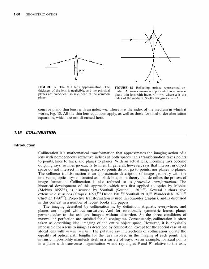
1 .60 GEOMETRIC OPTICS
FIGURE 17 The thin lens approximation . The thickness of the lens is negligible , and the principal planes are coincident , so rays bend at the common plane .
FIGURE 18 Reflecting surface represented un- folded . A convex mirror is represented as a convex- plano thin lens with index n 9 5 2 n , where n is the index of the medium . Snell’s law gives I 9 5 2 I .
concave plano thin lens , with an index 2 n , where n is the index of the medium in which it works , Fig . 18 . All the thin lens equations apply , as well as those for third-order aberration equations , which are not discussed here .
1 . 1 5 COLLINEATION
Introduction
Collineation is a mathematical transformation that approximates the imaging action of a lens with homogeneous refractive indices in both spaces . This transformation takes points to points , lines to lines , and planes to planes . With an actual lens , incoming rays become outgoing rays , so lines go exactly to lines . In general , however , rays that interest in object space do not intersect in image space , so points do not go to points , nor planes to planes . The collinear transformation is an approximate description of image geometry with the intervening optical system treated as a black box , not a theory that describes the process of image formation . Collineation is also referred to as projecti y e transformation . The historical development of this approach , which was first applied to optics by Mo ̈ bius (Mo ̈ bius 1855 1 9 2 ) , is discussed by Southall (Southall , 1910 1 9 3 ) . Several authors give extensive discussions (Czapski 1893 , 1 9 4 Drude 1901 1 9 5 Southall 1910 , 1 9 3 Wandersleb 1920 , 1 9 6
Chre ́ tien 1980 1 9 7 ) . Projective transformation is used in computer graphics , and is discussed in this context in a number of recent books and papers .
The imaging described by collineation is , by definition , stigmatic everywhere , and planes are imaged without curvature . And for rotationally symmetric lenses , planes perpendicular to the axis are imaged without distortion . So the three conditions of maxwellian perfection are satisfied for all conjugates . Consequently , collineation is often taken as describing ideal imaging of the entire object space . However , it is physically impossible for a lens to image as described by collineation , except for the special case of an afocal lens with m 5 m L 5 n / n 9 . The putative ray intersections of collineation violate the equality of optical path lengths for the rays involved in the imaging of each point . The intrinsic impossibility manifests itself in a variety of ways . As an example , for axial points in a plane with transverse magnification m and ray angles θ and θ 9 relative to the axis ,
GENERAL PRINCIPLES 1 .61
collineation gives m ~ tan θ / tan θ 9 , but optical path length considerations require that m ~ sin θ / sin θ 9 . Another violation is that of the skew invariant 6 5 n ( a y 2 b x ) . The ratio of this quantity before and after collineation is not unity , but 6 9 / 6 5 g 9 / g , where g is the axial direction cosine in object space and g 9 is that in image space .
The expressions for collineation do not contain refractive indices , another manifestation of their not accounting for optical path length . Rather than the refractive index ratio n 9 / n , which occurs in many imaging equations , the expressions of collineation involve ratios of focal lengths . For afocal lenses there are ratios of transverse and longitudinal magnifica- tions or ratios of the focal lengths of the lenses making up the afocal system .
The expressions for actual ray behavior take the form of collineation in the paraxial , and , more generally , parabasal limits . So paraxial calculations provide the coef ficients of the transformation for any particular system .
Collineation is most often treated by starting with the general form , and then reducing its complexity by applying the symmetries of a rotationally symmetric system , to give familiar simple equations such as Newton’s (Born & Wolf 1980 1 9 8 ) . Alternatively , it is possible to begin with the simple forms and to derive the general ones therefrom with a succession of images , along with translations and rotations . However , the more important use of these properties is in treating lenses lacking rotational symmetry . This includes those comprised of elements that are arbitrarily oriented , that is , tilted or decentered— either intentionally or unintentionally . Other examples are nonplanar objects , tilted object planes , and arbitrary three-dimensional object surfaces .
Lenses , along with plane mirror systems , can form a succession of images and can produce translations and rotations . Correspondingly , a succession of collinear transforma- tions is a collinear transformation , and these transformations form a group . It is associative , corresponding to the fact that a series of imaging operations can be associated pairwise in any way . There is a unit transformation , correspondingly physically to nothing or to a unit magnification afocal lens . There is an inverse , so an image distorted as a result of object or lens tilt can be rectified by an appropriately designed system—to the extent that collineation validly describes the ef fects .
General Equations
The general form of the collinear transformation is
x 9 5 a 1 x 1 b 1 y 1 c 1 z 1 d 1
ax 1 by 1 cz 1 d y 9 5
a 2 x 1 b 2 y 1 c 2 z 1 d 2
ax 1 by 1 cz 1 d z 9 5
a 3 x 1 b 3 y 1 c 3 z 1 d 3
ax 1 by 1 cz 1 d
(206)
At least one of the denominator coef ficients , a , b , c , d , is not zero . The equations can be inverted , so there is a one-to-one correspondence between a point ( x , y , z ) in object space and a point ( x 9 , y 9 , z 9 ) in image space . The inverted equations are formally identical , and can be written by replacing unprimed quantities with primed ones and vice versa in the above equation . It is seen that a plane is transformed to a plane , since a 9 x 9 1 b 9 y 9 1 c 9 z 9 1 d 9 5 0 has the same form as a function of ( x , y , z ) . An intersection of two planes gives a line . It can also be shown that a line transforms to a line by writing the equation for a line in parametric form , with parameter s , x ( s ) 5 x 0 1 a s , y ( s ) 5 y 0 1 b s , z ( s ) 5 z 0 1 g s . Substituting in the transformation equations , it is found that dx 9 / dy 9 5 ( dx 9 / d s ) / ( dy 9 / d s ) is constant , as are other such ratios .
These equations contain 16 coef ficients , but it is possible to divide all three equations through by one of the coef ficients , so there are 15 independent coef ficients in general . Since the location of an image point is described by three coordinates , five points that are not coplanar determine the transformation .
1 .62 GEOMETRIC OPTICS
The ratios of the coef ficient dimensions are determined by the fact that x , y , z and x 9 , y 9 , z 9 are lengths . A variety of schemes can be used and , in the expressions below , a given symbol may have dif ferent dimensions .
There are two major categories of the transformation , according to whether the denominator varies or is constant . That with a varying denominator corresponds to focal lenses . For afocal lenses , the demonimator is constant , and the general form of the transformation is
x 9 5 a 1 x 1 b 1 y 1 c 1 z 1 d 1 y 9 5 a 2 x 1 b 2 y 1 c 2 z 1 d 2 z 9 5 a 3 x 1 b 3 y 1 c 3 z 1 d 3
(207)
Here coef ficient d has been normalized to unity . Such a transformation is called af fine or telescopic .
Coordinate Systems and Degrees of Freedom
The transformation involves two coordinate systems . The origin of each is located by three parameters , as is the orientation of each . This leaves three parameters that describe the other aspects of the transformation for the most general case of no symmetry . The number is reduced to two if there is rotational symmetry .
In addition to considering the transformation of the entire space , there are other cases , especially the imaging of planes . In each situation , there are specific coordinate systems in which the aspects of the relationship , other than position and orientation , are most simply expressed . Accordingly , dif ferent coordinate systems are used in the following sections . Thus , for example , the z axis in one expression may not be the same as that for another .
Simplest Form of the General Transformation
For focal lenses , the denominators are constant for a set of parallel planes
ax 1 by 1 cz 1 d 5 constant (208)
Each such plane is conjugate to one of a set of parallel planes in the other space . Within each of these planes , the quantities x 9 / x , x 9 / y , x 9 / z are constant , as are the other such derivatives . Therefore , magnifications do not vary with position over these planes , although they do vary with direction . There is one line that is perpendicular to these planes in one space whose conjugate is perpendicular to the conjugate planes in the other space . It can be taken to be the z axis in one space and the z 9 axis in the other . The aximuths of the x - y and x 9 - y 9 axes are found by imaging a circle in each space , which gives an ellipse in the other . The directions of the major and minor axes determine the orientations of these coordinate axes . The principal focal planes , are the members of this family of planes for which
0 5 ax 1 by 1 cz 1 d (209)
Lines that are parallel in one space have conjugates that intersect at the principal focal plane in the other . The principal focal points are the intersection of the axes with the focal planes .

GENERAL PRINCIPLES 1 .63
Using these simplifying coordinate systems , the general transformation is
x 9 5 a 1 x
cz 1 d y 9 5
b 1 y
cz 1 d z 9 5
c 3 z 1 d 3
cz 1 d (210)
One of the six coef ficients can be eliminated , and two of the others are determined by the choice of origins for the z axis and z 9 axis . If the origins are taken to be at the principal focal points , the transformation equations are
x 9 5 e x x
z y 9 5
e y y
z z 9 5
e z
z (211)
where e x , e y , e z are constants . Unless e x 5 e y , the images of shapes in constant z planes vary with their orientations . Squares in one orientation are imaged as rectangles , and in others as parallelograms . Squares in planes not perpendicular to the axes are imaged , in general , with four unequal sides .
For afocal lenses , the simplest form is
x 9 5 m x x y 9 5 m y y z 9 5 m z z (212)
Spheres in one space are imaged as ellipsoids in the other . The principal axes of the ellipsoids give the directions of the axes for which the imaging equations are simplest .
Conjugate Planes
A pair of conjugate planes can be taken to have x 5 0 and x 9 5 0 , so the general transformation between such planes is
y 9 5 b 2 y 1 c 2 z 1 d 2
by 1 cz 1 d z 9 5
b 3 y 1 c 3 z 1 d 3
by 1 cz 1 d (213)
There are eight independent coef ficients , so four points that are not in a line define the transformation . In each space , two parameters specify the coordinate origins and one the orientation . Two parameters describe the other aspects of the transformation .
The simplest set of coordinates is found by a process like that described above . For focal lenses , constant denominators define a line set of parallel lines
by 1 cz 1 d 5 constant (214)
with similar conjugate lines in the other space . There is a line that is perpendicular to this family in one space , whose conjugate is perpendicular in the other , which can be taken as the z axis on one side and the z 9 axis on the other . There is a principal focal line in the plane in each space , and a principal focal point , at its intersection with the axis . In this coordinate system the transformation is
y 9 5 b 2 y
cz 1 d z 9 5
c 3 z 1 d 3
cz 1 d (215)
Of the five coef ficients , four are independent and two are fixed by the choice of origins . If z 5 0 and z 9 5 0 are at the principal focal points , then
y 9 5 e y y
z z 9 5
e z
z (216)
where e y and e z are constants .

1 .64 GEOMETRIC OPTICS
For afocal lenses , the general transformation between conjugate planes is
y 9 5 b 2 y 1 c 2 z 1 d 2 z 9 5 b 3 y 1 c 3 z 1 d 3 (217)
The simplest form of the transformation is
y 9 5 m y y z 9 5 m z z (218)
where m y and m z are constants .
Conjugate Lines
A line can be taken to have x 5 0 , y 5 0 , x 9 5 0 , y 9 5 0 , so its transformation is
z 9 5 c 3 z 1 d 3
cz 1 d (219)
There are three independent coef ficients , so three points determine them . The origins in the two spaces account for two of the parameters , leaving one to describe the relative scaling . The simplest forms are
Focal : z 9 5 e z
z Afocal : z 9 5 m z z (220)
There is a relationship between distances along a line (or ray) that is unchanged in collineation (Southall 1910 , 1 9 3 Southall 1933 1 9 9 ) . If four points on a line A , B , C , D have images A 9 , B 9 , C 9 , D 9 , the double ratio or cross ratio is invariant under projective transformation , that is ,
AC BC
BD AD
5 A 9 C 9
B 9 C 9
B 9 D A 9 D
(221)
where AC is the distance from A to C , and likewise for other pairs .
Matrix Representation of the Transformation
The transformation can be expressed in linear form by using the variables ( u 1 , u 2 , u 3 , u 4 ) and ( u 9 1 , u 9 2 , u 9 3 , u 9 4 ) , where x 5 u 1 / u 4 , y 5 u 2 / u 4 , z 5 u 3 / u 4 and x 9 5 u 9 1 / u 9 4 , y 9 5 u 9 2 / u 9 4 , z 9 5 u 9 3 / u 9 4 . These are referred to as homogeneous coordinates . The transformation can be written
1 u 9 1
u 9 2
u 9 3
u 9 4 2 5 1
a 1 b 1 c 1 d 1
a 2 b 2 c 2 d 2
a 3 b 3 c 3 d 3
a b c d 2 1
u 1
u 2
u 3
u 4
2 (222)
In terms of the cartesian coordinates and an additional pair of terms q and q 9 , the transformation can be expressed as
1 q 9 x 9
q 9 y 9
q 9 z 9
q 9 2 5 1
a 1 b 1 c 1 d 1
a 2 b 2 c 2 d 2
a 3 b 3 c 3 d 3
a b c d 2 1
qx
qy
qz
q 2 (223)

GENERAL PRINCIPLES 1 .65
The dimensions of q and q 9 depend on the choice of coef ficient dimensions . Here q 9 / q 5 ax 1 by 1 cz 1 d , the equation for the special set of planes .
Certain sections of the matrix are associated with various aspects the transformation (Penna & Patterson 1986 2 0 0 ) . The first three elements in the rightmost column have to do with translation . This is shown by setting ( x , y , z ) 5 (0 , 0 , 0) to locate the conjugate in the other space . The first three elements in the bottom row are related to perspective transformation . The upper left-hand 3 3 3 array expresses rotation , skew , and local magnification variation .
For the simple form of the transformation expressed in Eq . (211) , a 1 5 e x , b 2 5 e y , d 3 5 e z , c 5 1 , and the rest of the coef ficients vanish . The general matrix representation for the afocal transformation is
1 x 9
y 9
z 9
1 2 5 1
a 1 b 1 c 1 d 1
a 2 b 2 c 2 d 2
a 3 b 3 c 3 d 3
0 0 0 1 2 1
x
y
z
1 2 (224)
The quantities q and q 9 can also be included , in which case q 9 5 q . In the simplest afocal form , Eq . (212) , the matrix is diagonal with a 1 5 m x , b 2 5 m y , d 3 5 m z , and the rest of the nondiagonal coef ficients vanishing . A succession of collineations can be treated by multiplying the matrices that describe them (Chastang 1990 2 0 1 ) . To combine lenses with arbitrary orientations and to change coordinate systems , compatible rotation and transla- tion matrices are required . The transformation for a pure rotation with direction cosines ( L , M , N ) is
1 x 9
y 9
z 9
1 2 5 1
1 2 2 L 2
2 2 LM
2 2 LN
0
2 2 LM
1 2 2 M 2
2 2 MN
0
2 2 LN
2 2 MN
1 2 2 N 2
0
0 0 0 1 2 1
x
y
z
1 2 (225)
The transformation for translation by ( D x , D y , D z ) is
1 x 9
y 9
z 9
1 2 5 1
1 0 0 0 1 0 0 0 1 0 0 0
D x
D y
D z
1 2 1
x
y
z
1 2 (226)
The quantities q and q 9 can be included if necessary . The transformations associated with conjugate planes can likewise be expressed with 3 3 3 matrices , and the transforma- tions of lines with 2 3 2 matrices .
Rotationally Symmetric Lenses
For rotationally symmetric lenses , the simplest forms are obtained with the z and z 9 axes corresponding to the lens axis in the two spaces , and the x and x 9 meridians corresponding . There is one less degree of freedom than in the general case , and a 1 5 b 2 in Eq . (210) . The general transformation is thus
x 9 5 a 1 x
cz 1 d y 9 5
a 1 y
cz 1 d z 9 5
c 3 z 1 d 3
cz 1 d (227)
There are four degrees of freedom , two associated with the lens and two with the
1 .66 GEOMETRIC OPTICS
choice of coordinate origins . For focal lenses , the two axial length parameters are f and f 9 . If the coordinate origins are at the focal points ,
x 9 5 2 fx
z y 9 5 2
fy
z z 9 5
f 9 f
z (228)
If the coordinate origins are conjugate and related by magnification m 0 , then
x 9 5 m 0 x
1 1 z / f y 9 5
m 0 y
1 1 z / f z 9 5
( f 9 / f ) m 2 0 z
1 1 z / f (229)
The constant term in the numerator of the z 9 expression is the longitudinal magnification for z 5 0 , for which point dz 9 / dz 5 ( f 9 / f ) m 2
0 . A special case of these equations is that for which the principal points are the origins , so m 0 5 1 .
For rotationally symmetric afocal lenses , the two degrees of freedom are the transverse magnification m x 5 m y 5 m , and the longitudinal magnification m z 5 m L . The simplest set of transformation equations is
x 9 5 mx y 9 5 my z 9 5 m L z (230)
where z 5 0 and z 9 5 0 are conjugate . If m 5 Ú 1 and m L 5 Ú 1 the image space replicates object space , except possibly for orientation . If m L 5 m , the spaces are identical except for overall scaling and orientation . The m and m L appear as functions of ratios of focal lengths of the lenses that make up the afocal system .
Rays for Rotationally Symmetric Lenses
A skew ray with direction cosines ( a , b , g ) in object space is described in parametric form with parameter z as follows
x ( z ) 5 x 0 1 a
g z y ( z ) 5 x 0 1
b
g z (231)
For a focal lens , if z 5 0 is taken to be the front focal plane , and z 9 5 0 is the rear focal plane , the parametric form of the ray in image space is
x 9 ( z 9 ) 5 S 2 f a
g D 1 S 2
x 0
f 9 D z 9 y 9 ( z 9 ) 5 S 2 f
b
g D 1 S 2
y 0
f 9 D z 9 (232)
So x 9 0 5 2 f a / g , y 9 0 5 2 f b / g , a 9 / g 9 5 2 x 0 / f 9 , b 9 / g 9 5 2 y 0 / f 9 . For meridional rays with x 5 0 , if θ and θ 9 are the ray angles in the two spaces , then tan θ 5 b / g , tan θ 9 5 2 y 0 / f 9 , and
tan θ tan θ 9
5 f 9
f m (233)
where m is the transverse magnification in a plane where the meridional ray crosses the axis .
For afocal lenses , if z 5 0 and z 9 5 0 are conjugate planes , the ray in image space is given by
x 9 ( z 9 ) 5 mx 0 1 S m
m L
a
g D z 9 y 9 ( z 9 ) 5 my 0 1 S m
m L
b
g D z 9 (234)
For meridianal rays with x 5 0 , tan θ tan θ 9
5 m L
m (235)
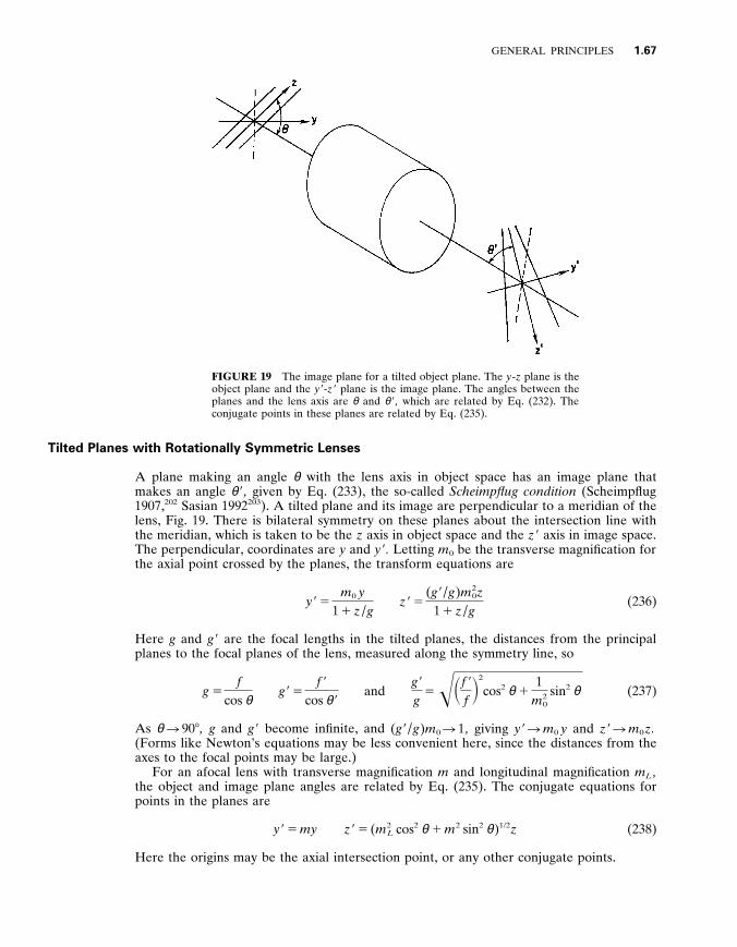
GENERAL PRINCIPLES 1 .67
FIGURE 19 The image plane for a tilted object plane . The y - z plane is the object plane and the y 9 - z 9 plane is the image plane . The angles between the planes and the lens axis are θ and θ 9 , which are related by Eq . (232) . The conjugate points in these planes are related by Eq . (235) .
Tilted Planes with Rotationally Symmetric Lenses
A plane making an angle θ with the lens axis in object space has an image plane that makes an angle θ 9 , given by Eq . (233) , the so-called Scheimpflug condition (Scheimpflug 1907 , 2 0 2 Sasian 1992 2 0 3 ) . A tilted plane and its image are perpendicular to a meridian of the lens , Fig . 19 . There is bilateral symmetry on these planes about the intersection line with the meridian , which is taken to be the z axis in object space and the z 9 axis in image space . The perpendicular , coordinates are y and y 9 . Letting m 0 be the transverse magnification for the axial point crossed by the planes , the transform equations are
y 9 5 m 0 y
1 1 z / g z 9 5
( g 9 / g ) m 2 0 z
1 1 z / g (236)
Here g and g 9 are the focal lengths in the tilted planes , the distances from the principal planes to the focal planes of the lens , measured along the symmetry line , so
g 5 f
cos θ g 9 5
f 9
cos θ 9 and
g 9
g 5 – S f 9
f D 2
cos 2 θ 1 1
m 2 0
sin 2 θ (237)
As θ 5 90 8 , g and g 9 become infinite , and ( g 9 / g ) m 0 5 1 , giving y 9 5 m 0 y and z 9 5 m 0 z . (Forms like Newton’s equations may be less convenient here , since the distances from the axes to the focal points may be large . )
For an afocal lens with transverse magnification m and longitudinal magnification m L , the object and image plane angles are related by Eq . (235) . The conjugate equations for points in the planes are
y 9 5 my z 9 5 ( m 2 L cos 2 θ 1 m 2 sin 2 θ ) 1 / 2 z (238)
Here the origins may be the axial intersection point , or any other conjugate points .
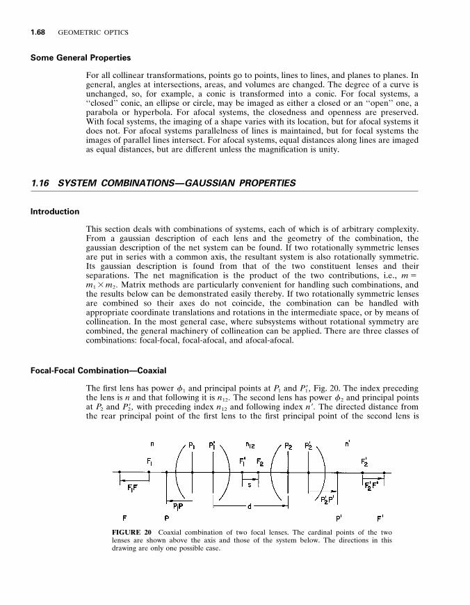
1 .68 GEOMETRIC OPTICS
Some General Properties
For all collinear transformations , points go to points , lines to lines , and planes to planes . In general , angles at intersections , areas , and volumes are changed . The degree of a curve is unchanged , so , for example , a conic is transformed into a conic . For focal systems , a ‘‘closed’’ conic , an ellipse or circle , may be imaged as either a closed or an ‘‘open’’ one , a parabola or hyperbola . For afocal systems , the closedness and openness are preserved . With focal systems , the imaging of a shape varies with its location , but for afocal systems it does not . For afocal systems parallelness of lines is maintained , but for focal systems the images of parallel lines intersect . For afocal systems , equal distances along lines are imaged as equal distances , but are dif ferent unless the magnification is unity .
1 . 1 6 SYSTEM COMBINATIONS — GAUSSIAN PROPERTIES
Introduction
This section deals with combinations of systems , each of which is of arbitrary complexity . From a gaussian description of each lens and the geometry of the combination , the gaussian description of the net system can be found . If two rotationally symmetric lenses are put in series with a common axis , the resultant system is also rotationally symmetric . Its gaussian description is found from that of the two constituent lenses and their separations . The net magnification is the product of the two contributions , i . e ., m 5 m 1 3 m 2 . Matrix methods are particularly convenient for handling such combinations , and the results below can be demonstrated easily thereby . If two rotationally symmetric lenses are combined so their axes do not coincide , the combination can be handled with appropriate coordinate translations and rotations in the intermediate space , or by means of collineation . In the most general case , where subsystems without rotational symmetry are combined , the general machinery of collineation can be applied . There are three classes of combinations : focal-focal , focal-afocal , and afocal-afocal .
Focal-Focal Combination—Coaxial
The first lens has power f 1 and principal points at P 1 and P 9 1 , Fig . 20 . The index preceding the lens is n and that following it is n 1 2 . The second lens has power f 2 and principal points at P 2 and P 9 2 , with preceding index n 1 2 and following index n 9 . The directed distance from the rear principal point of the first lens to the first principal point of the second lens is
FIGURE 20 Coaxial combination of two focal lenses . The cardinal points of the two lenses are shown above the axis and those of the system below . The directions in this drawing are only one possible case .
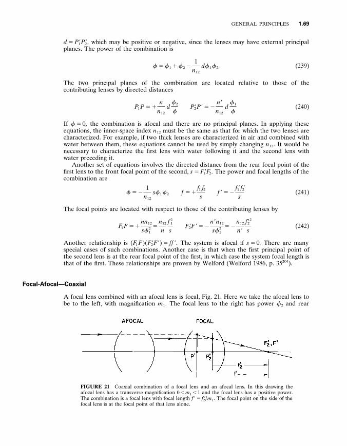
GENERAL PRINCIPLES 1 .69
d 5 P 9 1 P 9 2 , which may be positive or negative , since the lenses may have external principal planes . The power of the combination is
f 5 f 1 1 f 2 2 1
n 1 2 d f 1 f 2 (239)
The two principal planes of the combination are located relative to those of the contributing lenses by directed distances
P 1 P 5 1 n
n 1 2 d
f 2
f P 9 2 P 9 5 2
n 9
n 1 2 d
f 1
f (240)
If f 5 0 , the combination is afocal and there are no principal planes . In applying these equations , the inner-space index n 1 2 must be the same as that for which the two lenses are characterized . For example , if two thick lenses are characterized in air and combined with water between them , these equations cannot be used by simply changing n 1 2 . It would be necessary to characterize the first lens with water following it and the second lens with water preceding it .
Another set of equations involves the directed distance from the rear focal point of the first lens to the front focal point of the second , s 5 F 9 1 F 2 . The power and focal lengths of the combination are
f 5 2 1
n 1 2 s f 1 f 2 f 5 1
f 1 f 2
s f 9 5 2
f 9 1 f 9 2
s (241)
The focal points are located with respect to those of the contributing lenses by
F 1 F 5 1 nn 1 2
s f 2 1
5 n 1 2
n f 2
1
s F 9 2 F 9 5 2
n 9 n 1 2
s f 2 2
5 2 n 1 2
n 9
f 2 9 2
s (242)
Another relationship is ( F 1 F )( F 9 2 F 9 ) 5 ff 9 . The system is afocal if s 5 0 . There are many special cases of such combinations . Another case is that when the first principal point of the second lens is at the rear focal point of the first , in which case the system focal length is that of the first . These relationships are proven by Welford (Welford 1986 , p . 35 2 0 4 ) .
Focal-Afocal—Coaxial
A focal lens combined with an afocal lens is focal , Fig . 21 . Here we take the afocal lens to be to the left , with magnification m 1 . The focal lens to the right has power f 2 and rear
FIGURE 21 Coaxial combination of a focal lens and an afocal lens . In this drawing the afocal lens has a transverse magnification 0 , m 1 , 1 and the focal lens has a positive power . The combination is a focal lens with focal length f 9 5 f 9 2 / m 1 . The focal point on the side of the focal lens is at the focal point of that lens alone .

1 .70 GEOMETRIC OPTICS
FIGURE 22 Coaxial combination of two afocal lenses . An internal point A 9 has an object space conjugate A and an image space conjugate A 0 . These two points can be used for position references in the overall object and image spaces .
focal length f 9 2 . The power of the combination is f 2 m 1 , and the rear focal length of the combination is f 9 5 f 9 2 / m 1 . On the side of the focal lens , the location of the principal focal point is unchanged . On the side of the afocal lens , the system focal point is located at the image of the focal point of the focal lens in the space between the two . Changing the separation between the lenses does not change the power or the position of the principal focal point relative to that of the focal lens . The principal focal point on the afocal lens side does move .
Afocal-Afocal—Coaxial
The combination of two afocal lenses is itself afocal , Fig . 22 . If the two lenses have transverse magnifications m 1 and m 2 , the combination has m 5 m 1 m 2 . A pair of conjugate reference positions is found from the conjugates in the outer regions to any axial point in the inner space . If the separation between the two lenses changes , the combination remains afocal and the magnification is fixed , but the conjugate positions change . This result extends to a combination of any number of afocal lenses .
Noncoaxial Combinations—General
The most general combinations can be handled by the machinery of collineation . The net collineation can be found by multiplying the matrices that describe the constituents , with additional rotation and translation matrices to account for their relative positions . After obtaining the overall matrix , object and image space coordinate systems can be found in which the transformation is simplest . This approach can also be used to demonstrate general properties of system combinations . For example , by multiplying matrices for afocal systems , it is seen that a succession of afocal lenses with any orientation is afocal .
1 . 1 7 PARAXIAL MATRIX METHODS
Introduction
Matrix methods provide a simple way of representing and calculating the paraxial properties of lenses and their actions on rays . These methods contain no physics beyond that contained in the paraxial power and transfer equations , Eq . (136) and Eq . (142) , but they permit many useful results to be derived mechanically , and are especially useful for lens combinations . The matrix description of systems is also useful in elucidating fundamental paraxial properties . With the symbolic manipulation programs now available , matrix methods also provide a means of obtaining useful expressions .

GENERAL PRINCIPLES 1 .71
The optical system is treated as a black box represented by a matrix . The axial positions of the input and output planes are arbitrary . The matrix describes the relationship between what enters and what leaves , but contains no information about the specifics of the system within , and there is an infinity of systems with the same matrix representation .
The origin of matrix methods in optics is not clear . Matrices were used by Samson (Samson 1897 2 0 5 ) who referred to them as ‘‘schemes . ’’ Matrices appear without comment in a 1908 book (Leathem 1908 2 0 6 ) . Matrix methods are treated in papers (Halbach 1964 , 2 0 7
Sinclair 1973 2 0 8 ) and in many books (O 9 Neil 1963 , 2 0 9 Brouwer 1964 , 2 1 0 Blaker 1971 , 2 1 1
Longhurst 1973 , 2 1 2 Gerrard & Burch 1974 , 2 1 3 Naussbaum & Phillips 1976 , 2 1 4 Kogelnik 1979 , 2 1 5 Klein & Furtak 1986 , 2 1 6 Moller 1988 , 2 1 7 Guenther 1990 2 1 8 ) . Notation is not standardized , and many treatments are complicated by notation that conceals the basic structures .
This section is limited to rotationally symmetric lenses with homogeneous media . References are provided for systems with cylindrical elements . This treatment is monochromatic , with the wavelength dependence of index not made explicit .
The matrices are simplified by using reduced axial distances τ 5 t / n and reduced angles v 5 nu . The paraxial angles u are equivalent to direction cosines , and the reduced angles are optical direction cosines in the paraxial limit . For brevity , v and τ are usually referred to in this section simply as ‘‘angle’’ and ‘‘distance . ’’
Basic Idea—Linearity
Paraxial optics is concerned with the paraxial heights and paraxial angles of rays . A meridional ray entering a system has a given height y and angle v and leaves with another height y 9 and angle v 9 . Paraxial optics is linear , as discussed above , in the sense that both the outgoing height and angle depend linearly on the incoming height and angle . Writing Eq . (148) in terms of v 9 s gives
y 9 5 S y 9
y D y 1 S y 9
v D v and v 9 5 S v 9
y D y 1 S v 9
v D v (243)
The partial derivatives are constant for a given system . This linearity is the basis of the matrix treatment , since these equations can be written in matrix form :
1 y 9
v 9 2 5 1 y 9
y
v 9
y
y 9
v
v 9
v 2 1 y
v 2 (244)
Basic Operations
The basic operations in paraxial ray tracing are transfer , Eq . (136) , between surfaces and refraction or reflection at surfaces , Eq . (142) .
Transfer Matrix
Transfer changes the height of a ray , in general , leaving the angle unchanged . In terms of reduced quantities , the relationships are :
y 9 5 y 1 tu 5 y 1 t
n un 5 y 1 τ v and v 9 5 v (245)

1 .72 GEOMETRIC OPTICS
The transfer matrix is :
S 1 0
τ 1 D (246)
For left-to-right transfer , τ . 0 . This gives a dif ference in signs between some of the terms in expressions here and those in the gaussian section , where directed distances are measured from a reference point related to the lens to the object .
Power Matrix
Refraction or reflection changes the angle of a ray , but not its height . The equations for reduced quantities are
n 9 u 9 5 nu 2 y f 5 v 9 5 v 2 y f and y 9 5 y (247)
Here f 5 c ( n 9 2 n ) for refraction and f 5 2 2 nc for reflection , where c is the surface curvature , Eq . (143) . The power matrix is :
S 1 2 f
0 1 D (248)
A planar reflecting or refracting surface has f 5 0 , so it is represented by the unit matrix .
Arbitrary System
A general system consists of a series of surfaces with powers f 1 , f 2 , . . . that are separated from one another by distances τ 1 , τ 2 , . . . . Its matrix is the product
S 1 0
τ N
1 D ? ? ? S 1
2 f 2
0 1 D S 1
0 τ 2
1 D S 1
2 f 1
0 1 D S 1
0 τ 1
1 D (249)
By convention , the successive matrices are concatenated from right to left , whereas ray tracing is done left to right .
A special case is a succession of transfers , itself a transfer .
Succession of transfers : S 1 0
τ 1 1 τ 2 1 ? ? ?
1 D (250)
Another is a series of refractions with no intervening transfer , itself a power operation .
Succession of powers : S 1 2 ( f 1 1 f 2 1 ? ? ? )
0 1 D (251)
Matrix Elements
Each matrix element has a physical significance , and the terms can be given mnemonic symbols associated with the conditions under which they are zero . (This practice is not standard . ) If the initial ray angle is zero , the outgoing angles depend on the incident ray heights and the power of the system , according to v 9 5 2 f y , so v 9 / y 5 2 f . If the initial surface is at the front focal plane , the outgoing ray angles depend only on the incident

GENERAL PRINCIPLES 1 .73
height , so v 9 / v 5 0 . This term is denoted by F for ‘‘front . ’’ Similarly , if the final surface is at the real focal plane , the outgoing ray heights depend only on the incoming angles , so y 9 / y 5 R for ‘‘rear . ’’ If the initial and final planes are conjugate , then all incoming rays at a given height y have the outgoing height y 9 5 my , regardless of their angle , so y 9 / v 5 0 for conjugate planes . Since this term is related to the condition of conjugacy , y 9 / v 5 C for ‘‘conjugate . ’’ With this notation , the general matrix is
S R 2 f
C F D (252)
Dimensions
The terms R and F are dimensionless . C has the dimensions of length , and those of f are inverse length . Dimensional analysis , as well as the consideration of Eq . (248) , shows that the F and R terms will always contain products of equal numbers of f l ’s and τ k ’s , such as f k τ l . The f expression contains terms like f k and τ k f l f m , with one more power term than distance terms . Similarly , C has terms like τ k and τ k τ l f m .
Determinant
Both the transfer and power matrices have unit determinants . Therefore , any product of such matrices has a unit determinant , a fact that is related to the two-ray paraxial invariant .
U R 2 f
C F U 5 FR 1 C f 5 1 (253)
This provides an algebraic check . For afocal lenses and conjugate arrangements , FR 5 1 .
Possible Zeros
The possible arrangements of zeros in a system matrix is limited by the unit determinant restriction . There can be a single zero anywhere . In this case , either C 5 1 / f or F 5 1 / R , and the remaining nonzero term can have any value . There can be two zeros on either diagonal . No row or column can contain two zeros , since a system represented by such a matrix would violate conservation of brightness . A matrix with double zeros in the bottom row would collimate all rays , regardless of their incoming position and direction . A matrix with all zeros in the top row represents a system that would bring all incoming light to a single point . A system whose matrix has double zeros in the first column would bring all incoming light to a focus on the axis . For double zeros in the second row , the system would concentrate all light diverging from an input point in a single output point with a single direction .
Operation on Two Rays
Instead of considering a single input and output ray , the matrix formalism can be used to treat a pair of rays , represented by a 2 3 2 matrix . In this case
S y 9 1
v 9 1
y 9 2
v 9 2 D 5 S R
2 f
C
F D S y 1
v 1
y 2
v 2 D (254)

1 .74 GEOMETRIC OPTICS
Since the system matrix has a unit determinant , the determinants of the incoming and outgoing ray matrices are identical :
L 1 2 5 y 9 1 v 9 2 2 y 9 2 v 9 1 5 y 1 v 2 2 y 2 v 1 (255)
This is the paraxial invariant , Eq . (149) . It is possible to operate on more than two rays , but never necessary , since any third ray is a linear combination of two , Eq . (154) . Operations on two rays can also be handled with a complex notation in which two ray heights and two angles are each represented by a complex number (Marechal 1956 , 2 1 9
Marechal 1961 2 2 0 ) .
Conjugate Matrix
For conjugate planes , y 9 5 my , so C 5 0 , R 5 m , and F 5 1 / m , giving
S m 2 f
0 1 / m
D (256)
The 1 / m term gives the angular magnification , u 9 / u 5 n / n 9 m , Eq . (196) . This matrix also holds for afocal lenses , in which case f 5 0 .
Translated Input and Output Planes
For a given system , the locations of the input and output planes are arbitrary . If the input plane is translated by τ and the output plane by τ 9 , the resultant matrix is
S R 2 τ 9 f
2 f
C 1 τ R 1 τ 9 F 2 τ τ 9 f
F 2 τ f D (257)
Note that the object-space translation term τ is grouped with F and the image-space term τ 9 with R . The equation C 5 0 5 τ R 2 τ 9 F 2 τ τ 9 f gives all pairs of τ and τ 9 for which the input and output surfaces are conjugate .
Principal Plane-to-Principal Plane
If the input and output planes are the principal planes , then the matrix is a conjugate one , for which m 5 1 1 .
S 1 2 f
0 1 D (258)
This is also the matrix representing a thin lens .
Nodal Plane-to-Nodal Plane
The nodal points are conjugate , with unit angular magnification , so u 9 5 u and v 9 5 n 9 v / n . Thus
S n / n 9
2 f
0 n 9 / n
D (259)

GENERAL PRINCIPLES 1 .75
The transverse magnification m N 5 n / n 9 equals unity when n 5 n 9 . This matrix has no meaning for afocal lenses .
Focal Plane-to-Focal Plane
If the initial surface is at the front principal focal plane and the final surface is at the rear focal plane , the matrix is
S 0 2 f
1 / f 0 D (260)
This is the ‘‘Fourier transform’’ arrangement , in which incident heights are mapped as angles and vice versa .
Translation from Conjugate Positions
If the input plane is translated τ from a plane associated with magnification m and the output plane is translated a distance τ 9 from the conjugate plane , the matrix is
S m 2 τ 9 f
2 f
m τ 1 τ 9 / m 2 τ τ 9 f
1 / m 2 τ f D (261)
Setting C 5 0 gives an equation that locates all other pairs of conjugate planes relative to the first one , Eq . (172) .
Translation from Principal Planes
If the initial conjugate planes are the principal planes , then
S 1 2 τ 9 f
2 f
τ 1 τ 9 2 τ τ 9 f
1 2 τ f D (262)
The equation for other conjugates is C 5 0 5 τ 1 τ 9 2 τ τ 9 f , corresponding to Eq . (170) . It follows that the distance from the input surface to the first principal plane is τ 5 (1 2 F ) / f and the distance from the output surface to the second principal plane is τ 9 5 (1 2 R ) / f .
Translation from Focal Planes
If the input plane is a distance τ from the front focal plane and the output plane a distance τ 9 from the rear focal plane , the matrix is
1 2 f τ 9
2 f
1 f
(1 2 f 2 τ τ 9 )
2 f τ 2 (263)
Thus F and R are proportional to the distances of the input and output surfaces from the

1 .76 GEOMETRIC OPTICS
object space and image space focal planes . Using Newton’s formulas , this can also be written
1 m 9
2 f
1 f S 1 2
m 9
m D
1 m
2 (264)
Here m 9 is the magnification that would obtain if the image point were as located by R , and m is that if the object point were located by F . The conjugate term vanishes when m 5 m 9 .
Conjugate Relative to Principal Focal Planes
If Eq . (263) is a conjugate matrix , it becomes
S 2 f τ 9
2 f
0 2 f τ D (265)
The vanishing C term gives 0 5 1 / f 2 f τ τ 9 , which is the Newton equation usually written as zz 9 5 ff 9 . The magnification terms are the other Newton’s equations , m 5 2 f τ 9 and 1 / m 5 2 f τ , which are usually written as m 5 2 z 9 / f 9 5 2 f / z .
Afocal Lens
For afocal lenses f 5 0 . Since the determinant is unity , F 5 1 / R . And since the transverse magnification is constant , R 5 m , giving
S m
0 C
1 / m D (266)
A ray with v 5 0 has y 9 5 my , and v 9 5 v / m for all y . At conjugate positions , an afocal lens has the matrix
S m
0 0
1 / m D (267)
Performing a translation in both object and images spaces from the conjugate position gives
1 m
0
m τ 1 τ 9
m
1 / m 2 (268)
Setting C 5 0 gives τ 9 5 2 m 2 τ , which relates the location of a single conjugate pair to all others , Eq . (200) .

GENERAL PRINCIPLES 1 .77
Symmetrical Lenses
For lenses with symmetry about a central plane and symmetrically located input and output surfaces , F 5 R , so the matrix has the form
S B 2 f
C B D (269)
where B 2 5 1 2 f C . The conjugate matrix has m 5 Ú 1 .
Reversing Lenses
When a lens is flipped left to right , the matrix of the reversed system is obtained from that of the original one by switching the F and R terms .
S F
2 f
C
R D (270)
This reversal maintains the exterior references planes , that is , the input surface for the initial system becomes the output surface for the flipped one and vice versa .
Inverse Systems
By the ‘‘inverse’’ of a lens is meant a second system that undoes the ef fect of a given one . That is , the rays at the output surface of the second system have the same height and angle as those at the input of the first system . The combination of a system and its inverse is afocal with unit magnification . The matrix representing the inverse system is the inverse of that representing the system .
S F f
2 C R
D (271)
The matrix provides no instruction as to how such a lens is made up . Alternatively , the inverse matrix can be interpreted as that whose input is y 9 and v 9 , with outputs y and v .
Series of Arbitrary Lenses
The matrix for two successive lenses is
S R 1 R 2 2 C 2 f 1
2 f 1 F 2 2 f 2 R 1
C 1 R 2 1 C 2 F 1
F 1 F 2 2 C 1 f 2 D 5 S R 2
2 f 2
C 2
F 2 D S R 1
2 f 1
C 1
F 1 D (272)
For example , two given lenses separated by some distance have the matrix
S R 2
2 f 2
C 2
F 2 D S 1
0 τ 1 D S R 1
2 f 1
C 1
F 1 D (273)

1 .78 GEOMETRIC OPTICS
Multiplying from right to left gives a running product or ‘‘cumulative matrix , ’’ that shows the ef fect of the system up to a given plane .
Decomposition
Matrix multiplication is associative , so the system representation can be broken up in a number of ways . For example , the portion of a lens before and after the aperture stop can be used to find the pupil locations and magnifications . An arbitrary lens matrix can be written as a product of three matrices (Macukow & Arsenault 1983 2 2 1 ) :
S R 2 f
C F D 5 S 1
2 f / R 0 1 D S R
0 0
1 / R D S 1
0 C / R
1 D (274)
or
S R 2 f
C F D 5 S 1
0 C / F
1 D S 1 / F
0 0 F D S 1
2 f / F 0 1 D (275)
Thus a general lens is equivalent to a succession of three systems . One has power and works at unit magnification . The second is a conjugate afocal matrix . The third is a translation . Each of these systems is defined by one of the three terms , either R , f / R , C / R or F , f / F , C / F . This is another manifestation of the three degrees of freedom of paraxial systems .
Matrix Determination by Two-Ray Specification
If a two-ray input matrix is given along with the desired output , or the two input and output rays are measured to determine the matrix of an unknown lens , Eq . (254) gives
S R
2 f
C
F D 5 S y 9 1
v 9 1
y 9 2
v 9 2 D S y 1
v 1
y 2
v 2 D 2 1
(276)
so
S R 2 f
C F D 5
1 y 1 v 2 2 y 2 v 1
S y 9 1 v 2 2 y 9 2 v 1
v 9 1 v 2 2 v 9 2 v 1
y 9 2 y 1 2 y 9 1 y 2
v 9 2 y 1 2 y 2 v 9 1 D (277)
The denominator of the multiplicative factor is the paraxial invariant associated with the two rays , Eq . (149) . As a special case , the two rays could be the marginal and chief rays . The input and output pairs must have the same invariant , or the matrix thus found will not have a unit determinant .
Experimental Determination of Matrix Elements
The matrix elements for an unknown lens can , in principle , be determined experimentally . One method , as mentioned in the preceding section , is to measure the heights and angles of an arbitrary pair of rays . Another method is as follows . The power term is found in the usual way by sending a ray into the lens parallel to the axis and measuring its outgoing angle . To find C 5 y 9 / v , the input ray angle is varied , while its height is unchanged . If the output height is graphed , its slope is C . Likewise , the other partial derivatives in Eq . (243) can be found by changing one of the input parameters while the other is fixed . The four measurements are redundant , the unit determinant providing a check of consistency .
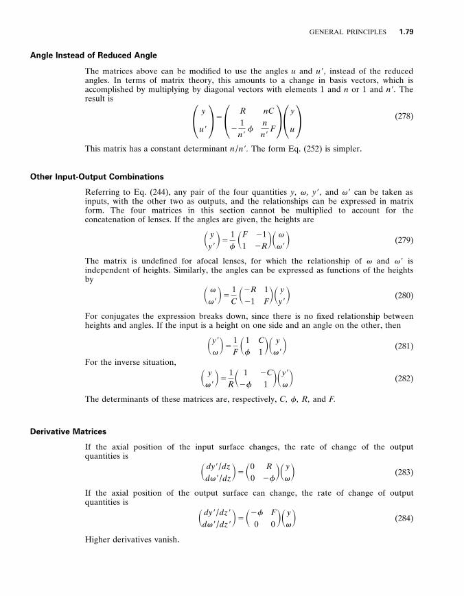
GENERAL PRINCIPLES 1 .79
Angle Instead of Reduced Angle
The matrices above can be modified to use the angles u and u 9 , instead of the reduced angles . In terms of matrix theory , this amounts to a change in basis vectors , which is accomplished by multiplying by diagonal vectors with elements 1 and n or 1 and n 9 . The result is
1 y
u 9 2 5 1 R
2 1
n 9 f
nC
n n 9
F 2 1 y
u 2 (278)
This matrix has a constant determinant n / n 9 . The form Eq . (252) is simpler .
Other Input-Output Combinations
Referring to Eq . (244) , any pair of the four quantities y , v , y 9 , and v 9 can be taken as inputs , with the other two as outputs , and the relationships can be expressed in matrix form . The four matrices in this section cannot be multiplied to account for the concatenation of lenses . If the angles are given , the heights are
S y y 9 D 5
1 f S F
1 2 1 2 R
D S v
v 9 D (279)
The matrix is undefined for afocal lenses , for which the relationship of v and v 9 is independent of heights . Similarly , the angles can be expressed as functions of the heights by
S v
v 9 D 5
1 C S 2 R
2 1 1 F D S y
y 9 D (280)
For conjugates the expression breaks down , since there is no fixed relationship between heights and angles . If the input is a height on one side and an angle on the other , then
S y 9
v D 5
1 F S 1
f
C 1 D S y
v 9 D (281)
For the inverse situation ,
S y v 9 D 5
1 R S 1
2 f
2 C 1 D S y 9
v D (282)
The determinants of these matrices are , respectively , C , f , R , and F .
Derivative Matrices
If the axial position of the input surface changes , the rate of change of the output quantities is
S dy 9 / dz d v 9 / dz
D 5 S 0 0
R 2 f
D S y v D (283)
If the axial position of the output surface can change , the rate of change of output quantities is
S dy 9 / dz 9
d v 9 / dz 9 D 5 S 2 f
0 F 0 D S y
v D (284)
Higher derivatives vanish .
1 .80 GEOMETRIC OPTICS
Skew rays
The matrix formalism can be used to treat a paraxial skew ray , represented by a 2 3 2 matrix of x and y positions and directions a and b . In this case
S x 9
n 9 a 9
y 9
n 9 b 9 D 5 S R
2 f
C F D S x
n a
y n b
D (285)
Since the lens matrix has a unit determinant , the determinants of the incoming and outgoing ray matrices are identical :
n 9 ( y 9 a 9 2 x 9 b 9 ) 5 n ( y a 2 x b ) (286)
From Eq . (73) , this is the skew invariant .
Relationship to Characteristic Functions
A lens matrix can be related to any one of the four paraxial characteristic functions , Eqs . (34) through (37) , each of which has three first coef ficients , associated with the three degrees of freedom of the matrix . Brouwer and Walther (Brouwer & Walther 1967 2 2 2 ) derive the paraxial matrices from more general matrices based on the point angle characteristic function .
Nonrotationally Symmetric Systems
Systems comprised of cylindrical lenses can also be treated paraxially by matrices (Arsenault 1979 , 2 2 3 Arsenault 1980 , 2 2 4 Arsenault 1980 , 2 2 5 Keating 1981 , 2 2 6 Arsenault & Macukow 1983 , 2 2 7 Macukow & Arsenault 1983 , 2 2 1 Attard 1984 2 2 8 ) . The more general case of a treatment around an arbitrary ray is also represented by a 4 3 4 matrix (Stone & Forbes 1992 2 2 9 ) . This is treated by several of the references to the section ‘‘Images About Known Rays . ’’
1 . 1 8 APERTURES , PUPILS , STOPS , FIELDS , AND RELATED MATTERS
Introduction
This section is concerned with the finite sizes of lens and their fields , as expressed in various limitations of linear dimensions and angles , and with some of the consequences of these limits . (Other consequences , for example , resolution limitations , are in the domain of wave optics . ) Terminology in this area is not well defined , and the terms typically used are insuf ficient for all the aspects of the subject , so this section deals considerably with definitions .
Field Size and Field Stop
The field or field of y iew of a lens is the region of object space from which light is captured or the region of image space that is used . The field size may be described in angular , linear , or area units , depending on the circumstances . (It can be described in still other ways , e . g ., the number of pixels . ) In and of itself , a lens does not have a definite field size , but
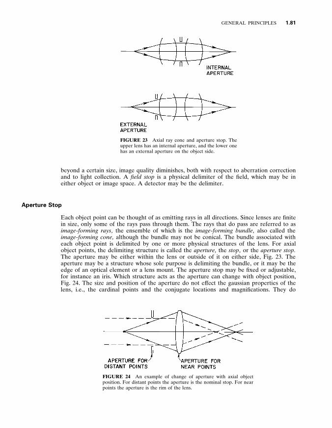
GENERAL PRINCIPLES 1 .81
FIGURE 23 Axial ray cone and aperture stop . The upper lens has an internal aperture , and the lower one has an external aperture on the object side .
beyond a certain size , image quality diminishes , both with respect to aberration correction and to light collection . A field stop is a physical delimiter of the field , which may be in either object or image space . A detector may be the delimiter .
Aperture Stop
Each object point can be thought of as emitting rays in all directions . Since lenses are finite in size , only some of the rays pass through them . The rays that do pass are referred to as image - forming rays , the ensemble of which is the image - forming bundle , also called the image - forming cone , although the bundle may not be conical . The bundle associated with each object point is delimited by one or more physical structures of the lens . For axial object points , the delimiting structure is called the aperture , the stop , or the aperture stop . The aperture may be either within the lens or outside of it on either side , Fig . 23 . The aperture may be a structure whose sole purpose is delimiting the bundle , or it may be the edge of an optical element or a lens mount . The aperture stop may be fixed or adjustable , for instance an iris . Which structure acts as the aperture can change with object position , Fig . 24 . The size and position of the aperture do not ef fect the gaussian properties of the lens , i . e ., the cardinal points and the conjugate locations and magnifications . They do
FIGURE 24 An example of change of aperture with axial object position . For distant points the aperture is the nominal stop . For near points the aperture is the rim of the lens .

1 .82 GEOMETRIC OPTICS
FIGURE 25 Schematic diagram of a lens with object and image planes , entrance and exit pupils , and marginal and chief rays . The entrance pupil is located at E and the exit pupil at E 9 . The chief ray passes through the edges of the fields and the centers of the pupils . The marginal ray passes through the axial object and image points and the edges of the pupils .
af fect the image irradiance , the aberrations , and the ef fects of defocus . The aperture is most commonly centered on axis , but this is not always so . With visual instruments , the aperture stop for the entire system may be either an aperture in the optics or the iris of the observer’s eye .
Marginal Rays and Chief Rays
Ray bundles are described to a considerable extent by specifying their central and extreme rays . For object planes perpendicular to the lens axis , there are two meridional rays of particular importance , defining the extremities of field and aperture , Fig . 25 . These rays are reciprocal in that one is to the pupil what the other is to the field .
The marginal ray originates at the axial object point , intersects the conjugate image point , and passes through the edge of the aperture . This term is also used for rays from other field points that pass through the extremes of the aperture . The paraxial marginal ray is the marginal ray in the paraxial limit .
The chief ray or principal ray originates at the edge of the object field , intersects the edge of the image field , and passes approximately through the center of the aperture , and hence approximately through the center of the pupils . (Here we use ‘‘chief ray , ’’ since the prefix ‘‘principal’’ is so commonly used for other entities . ) The term is also used for the central ray of other bundles . The paraxial chief ray passes exactly through the centers of the aperture and both paraxial pupils .
Field Angle
The field angle is that subtended by the field of view at the lens . This term is ambiguous , since several angles can be used , as well as angles in both object and image space . A nodal ray angle is the same in both spaces . If the nodal points are not at the pupils , the chief ray angle dif fers on the two sides . The ratio of paraxial chief ray angles is proportional to the paraxial pupil magnification , as discussed later , Eq . (289) . If the lens is telecentric , the chief ray angle is zero . An afocal lens has no nodal points , and the paraxial ratio of output angles to input angles is constant . The concept of field angle is most useful with objects and / or images at large distances , in which case on the long conjugate side the various ray angles are nearly identical . On the short conjugate side , ambiguity is removed by giving the
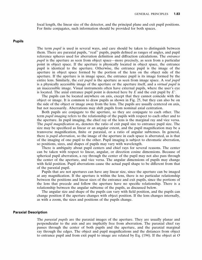
GENERAL PRINCIPLES 1 .83
focal length , the linear size of the detector , and the principal plane and exit pupil positions . For finite conjugates , such information should be provided for both spaces .
Pupils
The term pupil is used in several ways , and care should be taken to distinguish between them . There are paraxial pupils , ‘‘real’’ pupils , pupils defined as ranges of angles , and pupil reference spheres used for aberration definition and dif fraction calculations . The entrance pupil is the aperture as seen from object space—more precisely , as seen from a particular point in object space . If the aperture is physically located in object space , the entrance pupil is identical to the aperture . Otherwise , the entrance pupil is the image of the aperture in object space formed by the portion of the lens on the object side of the aperture . If the aperture is in image space , the entrance pupil is its image formed by the entire lens . Similarly , the exit pupil is the aperture as seen from image space . A real pupil is a physically accessible image of the aperture or the aperture itself , and a y irtual pupil is an inaccessible image . Visual instruments often have external pupils , where the user’s eye is located . The axial entrance pupil point is denoted here by E and the exit pupil by E 9 .
The pupils can be located anywhere on axis , except that they cannot coincide with the object or image . It is common to draw pupils as shown in Fig . 25 , but they can also be on the side of the object or image away from the lens . The pupils are usually centered on axis , but not necessarily . Aberrations may shift pupils from nominal axial centration .
Both pupils are conjugate to the aperture , so they are conjugate to each other . The term pupil imaging refers to the relationship of the pupils with respect to each other and to the aperture . In pupil imaging , the chief ray of the lens is the marginal ray and vice versa . The pupil magnification m P denotes the ratio of exit pupil size to entrance pupil size . The size may be specificed as linear or an angular extent , and the pupil magnification may be a transverse magnification , finite or paraxial , or a ratio of angular subtenses . In general , there is pupil aberration , so the image of the aperture in each space is aberrated , as is that of the imaging of one pupil to the other . Pupil imaging is subject to chromatic aberration , so positions , sizes , and shapes of pupils may vary with wavelength .
There is ambiguity about pupil centers and chief rays for several reasons . The center can be taken with respect to linear , angular , or direction cosine dimensions . Because of spherical pupil aberration , a ray through the center of the pupil may not also pass through the center of the aperture , and vice versa . The angular dimensions of pupils may change with field position . Pupil aberrations cause the actual pupil shape to be dif ferent from that of the paraxial pupil .
Pupils that are not apertures can have any linear size , since the aperture can be imaged at any magnification . If the aperture is within the lens , there is no particular relationship between the positions and linear sizes of the entrance and exit pupils , since the portions of the lens that precede and follow the aperture have no specific relationship . There is a relationship between the angular subtense of the pupils , as discussed below .
The angular size and shape of the pupils can vary with field position , and the pupils can change position if the aperture changes with object position . If the lens changes internally , as with a zoom , the sizes and positions of the pupils change .
Paraxial Description
The paraxial pupils are the paraxial images of the aperture . They are usually planar and perpendicular to the axis and are implicitly free from aberration . The paraxial chief ray passes through the center of both pupils and the aperture , and the paraxial marginal ray through the edges . The object and pupil magnifications and the distances from object to entrance pupil and from exit pupil to image are related by Eq . (194) . If the object at O

1 .84 GEOMETRIC OPTICS
is imaged at O 9 with magnification m , and the pupil magnification from entrance pupil at E to exit pupil at E 9 is m E , then from Eq . (194)
O 9 E 9 5 n 9
n mm E OE (287)
Paraxial Invariant for Full Field and Full Aperture
Let the height of the paraxial marginal ray be y M at the entrance pupil and y 9 M at the exit pupil , and that of the paraxial chief ray by y C , at the object plane and y 9 C at the image plane , Fig . 25 . Let the angles of these rays be u M , u C , u 9 M , u 9 C . The two-ray paraxial invariant , Eq . (149) , is
L 5 ny C u M 5 ny M u C 5 n 9 y 9 M u 9 C 5 n 9 y 9 C u 9 M (288)
This relationship was rediscovered several times , so the conserved quantity is referred to by a variety of names , including the Lagrange in y ariant , the Helmholtz in y ariant , the Smith in y ariant , and with various hyphenated combinations of the proper names (Rayleigh 1886 , 2 3 0 Southall 1910 2 3 1 ) . Further discussions are found in the sections on paraxial optics and on the e ́ tendue . The paraxial transverse magnification and paraxial pupil magnifica- tions are related to the paraxial marginal and chief ray angles by
m 5 y 9 C
y C 5
nu M
n 9 u 9 M and m P 5
y 9 M
y M 5
nu C
n 9 u 9 C (289)
Pupil Directions
For some purposes , pupils are best described as ranges of directions , specified in direction cosines , rather than by linear extents of aperture images . Here the term pupil directions (NS) is used . This is particularly the case when dealing with a given region of the object . The construction for this description is shown in Fig . 26 . The x and y axes of the
FIGURE 26 Construction for the description of the pupils with direction cosines . An x - y plane is tangent to the object surface at the object point , and a unit sphere is centered on the point . The intersections with the unit sphere of the rays are projected to the tangent plane to give the pupil direction cosines .

GENERAL PRINCIPLES 1 .85
object-space coordinate system lie in the object surface , and the x 9 and y 9 axes . From a point on the object plane , the extreme set of rays that passes through the lens is found . Its intersection with a unit sphere about the object point is found , and perpendiculars are dropped to the unit circle on (or tangent to) the object plane , giving the extent in direction cosines .
The entrance pupil is delimited by a closed curve described by a relationship 0 5 P ( a , b ; x , y ) , and the exit pupil is likewise defined by 0 5 P 9 ( a 9 , b 9 ; x 9 , y 9 ) . The spatial argument is included to indicate that the shape varies , in general , with the field position . There may be multiple regions , as in the case of central obstructions . It is usually preferable to define the pupils relative to principal directions (NS) ( a 0 , b 0 ) in object space and ( a 9 0 , b 9 0 ) in image space , where the two directions are those of the same ray in the two spaces , usually a meridional ray . The principal directions are analogous to the chief rays . The entrance pupil is then given by 0 5 Q ( a 2 a 0 , b 2 b 0 ; x , y ) and the exit pupil by 0 5 Q 9 ( a 9 2 a 9 0 , b 9 2 b 9 0 ; x 9 , y 9 ) . For example , for a field point on the x 5 0 meridian , the expression for the pupil might be well approximated by an ellipse , 0 5 a a 2 1 b ( b 2 b 0 )
2 , where (0 , b 0 ) is the chief ray direction . If the imaging is stigmatic , the relationship between entrance and exit pupil angular shapes is provided by the cosine condition , Eq . (104) .
Q 9 ( a 9 , b 9 ; x 9 , y 9 ) 5 Q ( m P a 9 2 a 9 0 , m P b 9 2 b 9 0 ; x , y ) (290)
The entrance and exit pupils have the same shapes when described in direction cosine space . They are scaled according to the pupil angular magnification (NS) m P 5 n / n 9 m . The orientations may be the same or rotated 180 8 . There is no particular relationship between ( a 0 , b 0 ) and ( a 9 0 , b 9 0 ) , which can , for example , be changed by field lenses . The principal directions are , however , usually in the same meridian as the object and image points , in which case a 0 / b 0 5 a 9 0 / b 9 0 . If the field point is in the x meridian , and the central ray is in this meridian , then a 0 5 0 and a 9 0 5 0 . Even with aberrations , Eq . (290) usually holds to a good approximation . The aberration pupil distortion refers to a deviation from this shape constancy .
Pupil Directional Extent : Numerical Aperture and Its Generalizations
The angular extent of a pupil extent is limited by some extreme directions . In the example above of the elliptical shape , for instance , there are two half widths
1 – 2 ( a m a x 2 a m i n ) and 1 – 2 ( b m a x 2 b m i n ) (291)
For a rotationally symmetric lens with a circular aperture , the light from an axial object point in a medium of index n is accepted over a cone whose vertex angle is θ m a x . The object space numerical aperture is defined as
NA 5 n sin θ m a x 5 n 4 ( a 2 1 b 2 ) max 5 n a m a x 5 n b m a x (292)
Likewise , on the image side , where the index is n 9 and the maximum angle is θ 9 m a x , the image space numerical aperture is
NA 9 5 n 9 sin θ 9 m a x 5 n 9 4 ( a 9 2 1 b 9 2 ) m a x 5 n 9 a 9 m a x 5 n 9 b 9 m a x (293)
1 .86 GEOMETRIC OPTICS
If the lens is free of coma , the sine condition , Eq . (106) , gives for finite conjugates
m 5 n sin θ m a x
n 9 sin θ 9 m a x 5
NA
NA 9 (294)
For infinite conjugates
sin θ 9 m a x 5 2 y m a x
f 9 or n 9 sin θ 9 m a x 5 NA 9 5 n b max 5 2 y m a x f (295)
If there is coma , these relationships are still good approximations . For a given lens and a given aperture size , the numerical aperture varies with the axial object position .
F-Number and Its Problems
The F - number is written in a variety of ways , including F / no . and F / 4 . It is denoted here by FN . The F-number is not a natural physical quantity , is not defined and used consistently in the literature , and is often used in ways that are both wrong and confusing (Hatch 1980 , 2 3 2 Goodman 1993 2 3 3 ) . Moreover , there is no need to use the F-number , since everything that it purports to describe or approximately describes is treated properly with direction cosines . The most common definition for F-number , applied to the case of an object at infinity , is
FN 5 focal length
entrance pupil diameter 5
1 2 tan θ 9
(296)
where θ 9 is the outgoing angle of the axial imaging done . In general , the F-number is associated with the tangents of collinear transformations , rather than the sines (or direction cosines) that are physically appropriate . It presumes that a nonparaxial ray entering parallel to the axis at height y leaves the rear principal plane at the same height and intersects the rear focal point , so that tan θ 9 5 y / f 9 . However , this particular presumption contradicts Eq . (294) , and in general , collineation does not accurately describe lens behavior , as discussed above .
Other problems with F-number , as it is used in the literature , include the following : (1) It is not defined consistently . For example , the literature also contains the definition F-number 5 (focal length) / (exit pupil diameter) . (2) For lenses used at finite conjugates , the F-number is often stated for an object at infinity . In fact , given only the numerical aperture for an object at infinity , that for other conjugates cannot be determined . (3) There are confusing descriptions of variation of F-number with conjugates , for example , the equation FN m 5 (1 1 m ) FN ̀ , where FN m is the F-number for magnification m and FN ̀
is that for an object at infinity . In fact , numerical apertures for various magnification are not so related . (4) The object and image space numerical apertures are related by Eq . (293) , but there is no such relationship for tangents of angles , except that predicted by collineation , Eq . (232) , which is approximate . (5) With of f-axis field points and noncircular pupils , the interpretation of F-number is more ambiguous . (6) Afocal systems have finite numerical apertures when used at finite conjugates , but they have no analogue to Eq . (295) . (7) Object and image space refractive indices are not accounted for by the F-number , whereas they are by the numerical aperture . (8) The F-number is often used as a descriptor of radiometric throughput , rather than of ray angles per se .
A related quantity is the T - number (W . J . Smith 1992 2 3 4 ) , which accounts for both the convergence angle of the imaging cone and the fraction of power transmitted by the lens .
GENERAL PRINCIPLES 1 .87
This is useful as a single-number descriptor , but it is subject to all the confusion associated with the F-number .
Image Irradiance for Lambertian Objects
If the light from a region of an object is lambertian with a power / area M , then the emitted power per angle with angle according to ( M / π ) cos θ d v 5 ( M / π ) d a d b . The power captured by the entrance pupil from a small object area dA is
dP 5 1 π
M dA E entrance pupil
d a d b (297)
(For a full hemisphere e d a d b 5 π , giving dP 5 M dA . ) If there are no losses within the lens , the power reaching the conjugate image region dA 9 is the same . Using the conservation of e ́ tendue equation , Eq . (72) , the image irradiance is
E 5 dP
dA 9 5
1 π
M n 9 2
n 2 E exit pupil
d a 9 d b 9 (298)
The image irradiance does not depend explicitly on the magnification , but magnification is included implicitly , since , for a given lens , the subtense of the exit pupil varies with conjugates .
This equation obtains everywhere in the field , and it applies to arbitrary object surface positions and orientations , so long as the direction cosines are defined with respect to the local object and image surface normals . These equations apply regardless of the chief ray angles , so they are applicable , for example , with telecentricity . In general , the pupil shape and principal direction vary with field position , so there is a gradation of irradiance in the image of a uniform lambertian object .
These equations do not account for all that influences image irradiance , for example lens absorption and reflection . These ef fects can be included in the above expressions by adding an appropriate weighting function of angle and field in the above integrals , giving
E ( x 9 , y 9 ) 5 dP
dA 9 5
1 π
M ( x , y ) n 9 2
n 2 E τ ( a 9 , b 9 ; x 9 , y 9 ) d a 9 d b 9 (299)
where τ ( a 9 , b 9 ; x 9 , y 9 ) is the lens transmittance as a function of the direction cosines for the image point ( x 9 , y 9 ) . With externally illuminated objects that are not lambertian scatterers , these relationships do not hold . For example , in optical projectors the illumination is matched to the object and imaging lens to give nominally uniform image irradiance .
Axial Image Irradiance for Lambertian Objects
In the special case of circular pupils and axial object surfaces perpendicular to the axis , the collected power and image irradiance given above are
dP 5 M dA sin 2 θ and E 5 M n 9 2
n 2 sin 2 θ 9 (300)

1 .88 GEOMETRIC OPTICS
Power / Pixel
From wave optics , a lens working at the ‘‘resolution limit’’ has an image pixel size q l / n 9 sin θ 9 , where l is the vacuum wavelength and q is a dimensionless factor , typically of the order of unity . Applying Eq . (300) , this gives
Power / pixel 5 q 2 M S l
n D 2
(301)
M ( l / n ) 2 is the energy emitted per square wavelength of object area . This is a fundamental radiometric quantity . Increasing q gives a greater numerical aperture than is nominally required for resolution , but in practice the aberration correction may be such that the actual resolution is not greater .
Cosine-to-the-Fourth Approximation
For distant , planar , uniform lambertian objects perpendicular to the lens axis , if the entrance pupil is well approximated by a circle , then the image irradiance varies approximately with the object space field angle c according to the cosine - to - the - fourth relationship
E ( c ) 5 E 0 cos 4 c (302)
where E 0 is the axial irradiance . There are three contributions to this dependence . (1) The angular distribution of a lambertian emitter varies as cos c . (2) The distance from the field point to the entrance pupil varies as 1 / d 2 ~ cos 2 c . (3) Insofar as the pupil behaves as a rigid circle , its projected solid angle varies approximately as cos c . The cosine-to-the- fourth relationship should be used only as a guideline , since ray tracing permits more accurate calculations , and because of the ambiguities in the meaning of the field angle , as discussed above , and elsewhere (Kingslake 1945 , 2 3 5 Reiss 1945 , 2 3 6 Gardner 1947 , 2 3 7 Reiss 1948 , 2 3 8 Kingslake 1965 2 3 9 ) . For example , field angle is meaningless with telecentricity . Some lenses , especially wide-angle ones , are specifically designed so the pupil subtense increases with the field angle in order to compensate for ef fects (1) and (2) above , to produce a suf ficiently uniform image (Slyusarev 1941 2 4 0 ) .
Total Lens E ́ tendue
The total amount of power from a lambertian object that can be transferred through a lens is
1 π
M E field
dx dy E pupil
d a d b (303)
The pupil integral may vary over the field . If the pupil is round and constant over the field , the e ́ tendue is proportional to A(NA) 2 , where A is the area of the field . This quantity is also related to the total number of pixels in the field , and the ability of the lens to transfer information (Gabor 1961 2 4 1 ) . The term ‘‘area-solid angle product’’ is sometimes used , but this is an approximation . The total etendue is proportional paraxially to , L 2 , where L is given by Eq . (288) .

GENERAL PRINCIPLES 1 .89
FIGURE 27 Example of vignetting . The dashed ray passes through the aperture , but misses the lens .
Vignetting
Vignetting occurs when an image-forming bundle is truncated by two or more physical structures in dif ferent planes , Fig . 27 . Typically , one is the nominal aperture and another is the edge of a lens . Another case is that of central obstructions away from the aperture . When vignetting occurs , the image irradiance is changed , and its diminution with field height is faster than it otherwise would be . Aberration properties are also changed , so vignetting is sometimes used to eliminate light that would unacceptably blur the image .
Lens Combinations and Field Lenses
When lenses are used to relay images , the light is transferred without loss only if the exit pupil of one corresponds with the entrance pupil of the next . An example of the failure to meet this requirement is shown in Fig . 28 . The axial point is reimaged satisfactorily , but of f-axis bundles are vignetted . To transfer the light properly , a field lens in the vicinity
FIGURE 28 A pair of lenses relaying an image with and without a field lens . In the top figure , there is no field lens , and some of the light forming the intermediate image does not pass through the second lens . The amount lost depends on the two numerical apertures and increases with distance from the axis . In the lower figure , a field lens at the intermediate image forms an image of the exit pupil of the first lens into the entrance pupil of the next . No light is lost unless the numerical aperture of the second lens is less than that of the first .

1 .90 GEOMETRIC OPTICS
of the intermediate image is used to image the exit pupil of the preceding lens into the entrance pupil of the next one . If the field lens is a thin lens in the image plane , then its magnification with respect to the image is unity . In practice , the field lens is usually shifted axially , so scratches or dust on its surface are out of focus . Its magnification then dif fers from unity . The focal length of a thin field lens in air is given by 1 / f 9 5 1 / a 1 1 / b , where a is the distance from exit pupil of first lens to the field lens , and b is that from field lens to the entrance pupil of the second lens . The exit pupil is reimaged with a magnification b / a . If the sizes of the various pupils and their images are not matched , then the aperture of the combination is determined by the smallest . Field lenses af fect aberrations .
Defocus
When the object and image-receiving surface are not conjugate there is defocus . If either the object or the receiving surface is considered to be correctly positioned , the defocus is associated with the other . Another situation is that in which the object and receiving surfaces are conjugate , but both are wrongly located , so that the image is sharp but the magnification is not what is desired , a condition that might be called misfocus (NS) .
Defocus has two basic geometric ef fects , if there are no aberrations , Fig . 29 . One is blurring , since the rays from an object point do not converge to a single point on the receiving surface . The blur size varies linearly with the axial defocus in image space and with the cone angle of the image-forming bundle . The shape of the blur is that of the exit pupil , projected on the receiving surface . The other ef fect of defocus is a lateral shift in position of the blur’s centroid relative to that of the correctly focused point . The shift depends on the chief ray angle on the side of the lens where the defocus occurs . In the simplest case , the shift is approximately linear with field height , so acts as a change of magnification . If the object is tilted or is not flat , the ef fects of defocus vary across the field in a more complicated way . Aberrations af fect the nature of the blur . With some aberrations , the blur is dif ferent on the two sides of focus . With spherical aberration , the blur changes in quality , and with astigmatism the orientation of the blur changes .
In considering the geometrical imaging of a small region of a lambertian object , there is an implict assumption that the pupil is filled uniformly with light . In imaging an extended object that is externally illuminated , the light from a given region may not fill the pupil uniformly , so the character of the blurring is af fected by the angular properties of the illumination and scattering properties of the object .
The amount of defocus can be described in either object or image space , and it can be measured in a variety of ways , for example , axial displacement , displacement along a chief ray , geometrical blur size , and wavefront aberration . The axial displacements in object
FIGURE 29 Defocus of the receiving surface . A receiving surface is shown in focus and shifted axially . The image of a point on the shifted surface is blurred , and its centroid is translated radially .
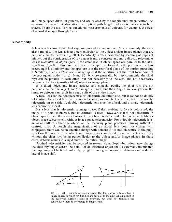
GENERAL PRINCIPLES 1 .91
and image space dif fer , in general , and are related by the longitudinal magnification . As expressed in wavefront aberration , i . e ., optical path length , defocus is the same in both spaces . There are also various functional measurements of defocus , for example , the sizes of recorded images through focus .
Telecentricity
A lens is telecentric if the chief rays are parallel to one another . Most commonly , they are also parallel to the lens axis and perpendicular to the object and / or image planes that are perpendicular to the axis , Fig . 30 . Telecentricity is often described by speaking of pupils at infinity , but the consideration of ray angles is more concrete and more directly relevant . A lens is telecentric in object space if the chief rays in object space are parallel to the axis , a 0 5 0 and b 0 5 0 . In this case the image of the aperture formed by the portion of the lens preceding it is at infinity and the aperture is at the rear focal plane of the portion preceding it . Similarly , a lens is telecentric in image space if the aperture is at the front focal point of the subsequent optics , so a 9 0 5 0 and b 9 0 5 0 . More generally , but less commonly , the chief rays can be parallel to each other , but not necessarily to the axis , and not necessarily perpendicular to a (possibly tilted) object or image plane .
With tilted object and image surfaces and nonaxial pupils , the chief rays are not perpendicular to the object and / or image surfaces , but their angles are everywhere the same , so defocus can result in a rigid shift of the entire image .
A focal lens can be nontelecentric or telecentric on either side , but it cannot be doubly telecentric . An afocal lens can be nontelecentric , or doubly telecentric , but it cannot be telecentric on one side . A doubly telecentric lens must be afocal , and a singly telecentric lens cannot be afocal .
For a lens that is telecentric in image space , if the receiving surface is defocused , the image of a point is blurred , but its centroid is fixed . However , if it is not telecentric in object space , then the scale changes if the object is defocused . The converse holds for object-space telecentricity without image-space telecentricity . For a doubly telecentric lens , an axial shift of either the object or the receiving plane produces blurring without a centroid shift . Although the magnification of an afocal lens does not change with conjugates , there can be an ef fective change with defocus if it is not telecentric . If the pupil is not on the axis or if the object and image planes are tilted , there can be telecentricity without the chief rays being perpendicular to the object and / or image planes . In these cases , defocus results in a rigid shift of the entire image .
Nominal telecentricity can be negated in several ways . Pupil aberrations may change the chief ray angles across the field . For an extended object that is externally illuminated the pupil may not be filled uniformly by light from a given region , so defocus can product a lateral image shift .
FIGURE 30 Example of telecentricity . The lens shown is telecentric in image space , in which ray bundles are parallel to the axis . An axial shift in the receiving surface results in blurring , but does not translate the centroid , so there is no change in image scale .

1 .92 GEOMETRIC OPTICS
Depth of Focus and Depth of Field
The depth of focus and depth of field are the amounts of defocus that the receiving surface or object may undergo before the recorded image becomes unacceptable . The criterion depends on the application—the nature of the object , the method of image detection , and so on , and there are both ray and wave optics criteria for goodness of focus . For example , a field of separated point objects dif fers from that of extended objects . Depth of focus is usually discussed in terms of blurring , but there are cases where lateral shifts become unacceptable before blurring . For example , in nature photography blurring is more critical than geometrical deformation , while the opposite may be true in metrology .
Range of Focus and Hyperfocal Distance
In some cases , a geometrical description of defocus is applicable , and the allowable blur is specified as an angle (Ray 1988 , 2 4 2 Kingslake 1992 , 2 4 3 W . Smith 1992 2 3 4 ) . The hyperfocal distance is
Hyperfocal distance 5 diameter of the entrance pupil
maximum acceptable angular blur 5 d H (304)
Let the object distance at which the lens is focused be d , the nearest distance at which the image is acceptable be d N , and the furthest distance be d F . All of these quantities are positive definite . The following relations obtain :
d F 5 d H d
d H 2 d and d N 5
d H d
d H 1 d (305)
The distances to either side of best focus are
d F 2 d 5 d 2
d H 2 d and d 2 d N 5
d 2
d H 1 d (306)
The total range of focus is
d F 2 d N 5 2 d 2 d H
d 2 H 2 d 2 5
2 d
( d H / d ) 2 2 1 (307)
For d . d H the above quantities involving d F are infinite (not negative) . If the lens is focused at the hyperfocal distance or beyond , then everything more distant is adequately focused . If the lens is focused at the hyperfocal distance , i . e ., d 5 d H , the focus is adequate everywhere beyond half this distance , and this setting gives the greatest total range . If the lens is focused at infinity , then objects beyond hyperfocal distance are adequately focused . The hyperfocal distance decreases as the lens is stopped down .
1 . 1 9 GEOMETRIC ABERRATIONS OF POINT IMAGES — DESCRIPTION
Introduction
In instrumental optics , the term aberration refers to a departure from what is desired , whether or not it is physically possible . Terms such as ‘‘perfect system’’ and ‘‘ideal system’’ indicate what the actual is compared to , and these terms themselves are not absolute , but depend on what is wished for . The ideal may be intrinsically impossible , in which case a deviation therefrom is not a defect . A further distinction is between aberrations inherent in a design and those that result from shortcomings in fabrication .
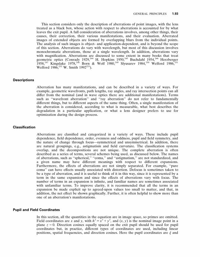
GENERAL PRINCIPLES 1 .93
This section considers only the description of aberrations of point images , with the lens treated as a black box , whose action with respect to aberrations is accounted for by what leaves the exit pupil . A full consideration of aberrations involves , among other things , their causes , their correction , their various manifestations , and their evaluation . Aberrated images of extended objects are formed by overlapping blurs from the individual points . The analysis of such images is object- and application-dependent , and is beyond the scope of this section . Aberrations do vary with wavelength , but most of this discussion involves monochromatic aberrations , those at a single wavelength . In addition , aberrations vary with magnification . Aberrations are discussed to some extent in many books that treat geometric optics (Conrady 1929 , 2 4 4 H . Hopkins 1950 , 2 4 5 Buchdahl 1954 , 2 4 6 Herzberger 1958 , 2 4 7 Kingslake 1978 , 2 4 8 Born & Wolf 1980 , 2 4 9 Slyusarev 1984 , 2 5 0 Welford 1986 , 2 5 1
Welford 1986 , 2 5 2 W . Smith 1992 2 5 3 ) .
Descriptions
Aberration has many manifestations , and can be described in a variety of ways . For example , geometric wavefronts , path lengths , ray angles , and ray intersection points can all dif fer from the nominal (and in wave optics there are additional manifestations) . Terms such as ‘‘wavefront aberration’’ and ‘‘ray aberration’’ do not refer to fundamentally dif ferent things , but to dif ferent aspects of the same thing . Often , a single manifestation of the aberration is considered , according to what is measurable , what best describes the degradation in a particular application , or what a lens designer prefers to use for optimization during the design process .
Classification
Aberrations are classified and categorized in a variety of ways . These include pupil dependence , field dependence , order , evenness and oddness , pupil and field symmetry , and the nature of change through focus—symmetrical and unsymmetrical . In addition , there are natural groupings , e . g ., astigmatism and field curvature . The classification systems overlap , and the decompositions are not unique . The complete aberration is often described as a series of terms , several schemes being used , as discussed below . The names of aberrations , such as ‘‘spherical , ’’ ‘‘coma , ’’ and ‘‘astigmatism , ’’ are not standardized , and a given name may have dif ferent meanings with respect to dif ferent expansions . Furthermore , the ef fects of aberrations are not simply separated . For example , ‘‘pure coma’’ can have ef fects usually associated with distortion . Defocus is sometimes taken to be a type of aberration , and it is useful to think of it in this way , since it is represented by a term in the same expansion and since the ef fects of aberrations vary with focus . The number of terms in an expansion is infinite , and familiar names are sometimes associated with unfamiliar terms . To improve clarity , it is recommended that all the terms in an expansion be made explicit up to agreed-upon values too small to matter , and that , in addition , the net ef fect be shown graphically . Further , it is often helpful to show more than one of an aberration’s manifestations .
Pupil and Field Coordinates
In this section , all the quantities in the equation are in image space , so primes are omitted . Field coordinates are x and y , with h 2 5 x 2 1 y 2 , and ( x , y ) is the nominal image point in a plane z 5 0 . Direction cosines equally spaced on the exit pupil should be used for pupil coordinates but , in practice , dif ferent types of coordinates are used , including linear positions , spatial frequencies , and direction cosines . Here the pupil coordinates are j and

1 .94 GEOMETRIC OPTICS
h , which are dimensionless , with r 2 5 j 2 1 h 2 . The overall direction of the pupil may vary with field . Here the ( j , h ) 5 (0 , 0) is always taken at the pupil center , the meaning of which may not be simple , as discussed in the section on pupils above . The angle of a meridian in the pupil is c . Entrance and exit pupil coordinates must be distinguished . For dif fraction calculations , the exit pupil should be sampled at equal intervals in direction cosines , but a set of rays from an object point that is equally spaced in direction cosines may leave with uneven spacing , as a result of aberrations .
Wavefront Aberration
If an object point is imaged stigmatically , then the optical path lengths of all rays from the object point to its image are identical , and the geometric wavefronts leaving the exit pupil are spherical . In the presence of aberrations , the wavefront is no longer spherical . Rather than describing the wavefront shape , it is usually preferable to consider the dif ference between the actual wavefront , and a nominal wavefront , often called the reference sphere , centered at a reference point that is usually the nominal image point . This reference sphere is usually taken to intersect the center of the pupil , since this gives the most accurate dif fraction calculations . The wa y efront aberration W is the optical path length from reference sphere to wavefront , or vice versa , according to the convention used , Fig . 31 . Two sign conventions are in use ; a positive wavefront aberration may correspond either to a wavefront which lags or leads the reference sphere . For each nominal image point ( x , y , z ) , the wavefront aberration is a function of the pupil coordinates ( j , h ) , so the functional form is W ( j , h ; x , y , z ) , with the z usually suppressed , since the image plane is usually taken to be fixed . For a given lens prescription , W is found by tracing a set of rays from each object point to the reference sphere and calculating their path lengths . If the absolute path length is unimportant , the choice of the reference sphere’s radius is not critical . Considered from the point of view of wave optics , the image of a point is degraded by phase dif ferences across the reference sphere , so absolute phase is of no consequence , and the zero of the wavefront aberration can be chosen arbitrarily . By convention and convenience , the zero is usually taken at the center of the pupil , so W (0 , 0 , x , y ) 5 0 .
FIGURE 31 Wavefront aberration . The reference sphere is concentric with the nominal image point . The wavefront is taken that is tangent to the reference sphere in the center of the pupil . The wavefront aberration function is the distance from the reference sphere to the wavefront as a function of pupil coordiantes .

GENERAL PRINCIPLES 1 .95
Absolute optical path lengths are significant for imaging systems with paths that separate between object and image in cases where there is coherence between the various image contributions . An error in absolute optical path length is called piston error . This results in no ray aberrations , so it is omitted from some discussions .
Ray Aberrations
In the presence of aberrations , the rays intersect any surface at dif ferent points than they would otherwise . The intersection of the rays with the receiving surface , usually a plane perpendicular to the axis , is most often of interest . The trans y erse ray aberration is the vectorial displacement ( » x , » y ) between a nominal intersection point and the actual one . The displacement is a function of the position of the nominal image point ( x , y ) and the position in the pupil through which the ray passes ( j , h ) . A complete description of transverse ray aberrations is given by
» x ( j , h ; x , y ) and » y ( j , h ; x , y ) (308)
The longitudinal aberration is the axial displacement from nominal of an axial intersection point . This description is useful for points on the axis of rotationally symmetrical systems , in which case all rays intersect the axis . Such aberrations have both transverse and longitudinal aspects . The intersection with a meridian can also be used . The diapoint is the point where a ray intersects the same meridian as that containing the object point (Herzberger 1958 2 4 7 ) . For an image nominally located at infinity , aberrations can be described by the slope of the wavefront relative to that of the nominal , that is , by ray angles rather than intersection points . A hypothetical ideal focusing lens can also be imagined to convert to transverse aberrations .
A ray intercept diagram shows the intersection points of a group of rays with the receiving surface (O’Shea 1994 2 5 4 ) . The rays are usually taken to arise from a single object point and to uniformly sample the pupil , with square or hexagonal arrays commonly used . The ray intercept diagrams can suf fer from artifacts of the sampling array , which can be checked for by using more than one type of array . Other pupil loci , for instance , principal meridians and annuli , can be employed to show particular aspects of the aberration . Intercept diagrams can also be produced for a series of surfaces through focus . Image quality may be better than ray diagrams suggest , since destructive interference can reduce the irradiance in a region relative to that predicted by the ray density .
Relationship of Wavefront and Ray Aberrations
Since rays are normal to geometric wavefronts , Fig . 32 , transverse ray aberrations are proportional to the slope of the wavefront aberration function . For systems of rotation
FIGURE 32 Ray aberration . Rays intersect the receiving plane at positions shifted from the nominal .
1 .96 GEOMETRIC OPTICS
with image space index n and marginal ray angle θ , the transverse aberrations are to a good approximation (Welford 1986 2 5 1 )
» x 5 1
n sin θ W
j » y 5
1 n sin θ
W
h (309)
The refractive index appears since W is an optical path length . If the rays are nominally parallel , then the partial derivatives give the angular ray errors
D a 5 1
np
W
j D b 5
1 np
W
h (310)
where p is the linear radius of the exit pupil , which cannot be infinite if the image is at infinity . These expressions may also have a multiplicative factor of 2 1 , depending on the sign conventions . A sum of wavefront aberrations gives a transverse aberration that is the sum of the contributing ones .
Ray Densities
The density of rays near the nominal image point is (Welford 1986 2 5 1 )
1 Density
~ S 2 W
j 2 D S 2 W
h 2 D 2 2 S 2 W
j h D 2
(311)
Caustics are the surfaces where ray densities are infinite . Here , geometric optics predicts infinite power / area , so the ray model is quantitatively inaccurate in this case .
Change of Reference Points
The center of the reference sphere may be displaced from the nominal image point . If the reference point is changed by linear displacement ( d x , d y , d z ) , then the wavefront aberration function changes from W to W 9 according to
W 9 ( j , h ; x , y ; d x , d y , d z ) 5 W ( j , h ; x , y ) 1 W x j 1 W y h 1 W z ( j 2 1 h 2 ) (312)
where W x 5 n sin θ d x ,
W y 5 n sin θ d y (313)
W z 5 1 – 2 n sin 2 θ d z
The transverse ray aberration » 9 x and » 9 y with respect to the new reference points are
» 9 x 5 » x 1 d x 1 sin θ d z » 9 y 5 » y 1 d y 1 sin θ d z (314)
The change through focus is accounted for by varying d z . Setting » 9 x 5 » 9 y 5 0 gives the
GENERAL PRINCIPLES 1 .97
parametric equations x ( d z ) and y ( d z ) for a ray with pupil coordinates ( j , h ) , relative to the nominal ray near the nominal image point .
Aberration Symmetries for Systems with Rotational Symmetry
If the lens , including the aperture , is a figure of rotation , only certain aberration forms are possible . For object points on axis , the wavefront aberration and the image blur are figures of revolution . For of f-axis points , both wavefront aberration and blur are bilaterally symmetrical about the meridional plane containing the object point . For object points on a circle centered on the axis , the wavefront and ray aberrations are independent of azimuth , relative to the local meridian . In practice , there is always some imperfection , so the symmetries are imperfect and additional aberration forms arise .
Wavefront Aberration Forms for Systems with Rotational Symmetry
Here the pupil is taken to be circular , with the coordinate zero taken at the center . The field coordinates are normalized so x 2 1 y 2 5 h 2 5 1 at the edge of the field . The pupil coordinates are normalized , so that j 2 1 h 2 5 r 2 5 1 on the rim of the pupil . The algebra is simplified by using dimensionless coordinates . To add dimensions and actual sizes , replace the j by j / j max , and likewise for other variables . The simplest combinations of pupil and field coordinates with rotational symmetry are
x 2 1 y 2 5 h 2 j 2 1 h 2 5 r 2 j x 1 h y (315)
The general wavefront aberration function can be expressed as a series of such terms raised to integral powers ,
W ( x , y ; j , h ) 5 O L ,M ,N 5 0
W L M N ( x 2 1 y 2 ) L ( j 2 1 h 2 ) M ( x j 1 y h ) N (316)
where L , M , N are positive integers . The terms can be grouped in orders according to the sum L 1 M 1 N , where , by convention , the order equals 2( L 1 M 1 N ) 2 1 . The order number refers more directly to ray aberration forms than to wavefront forms , and it is always odd . The first-order terms are those for which L 1 M 1 N 5 1 , for the third-order terms the sum is two , and so on . The number of terms in the Q th order is 1 1 ( Q 1 1)( Q 1 7) / 8 . For orders 1 , 3 , 5 , 7 , 9 the number of terms is 3 , 6 , 10 , 15 , 21 . For each order , one contribution is a piston error , which is sometimes excluded from the count .
The expression of Eq . (316) is related to the characteristic function for a rotationally symmetrical system , Eq . (32) . If the spatial coordinates are taken to be those of the object point , this is the point-angle characteristic function . In the hamiltonian optics viewpoint , the characteristic function is a sum of two parts . The first-order terms specify the nominal properties , and those of higher orders the deviation therefrom . This is discussed in the references given in that section . The term for which L 5 M 5 N 5 0 has to do with absolute optical path length .
Since there is bilateral symmetry about all meridians , the expansion can be simplified by considering object points in a single meridian , customarily taken to be that for which x 5 0 . Doing so and letting the fractional field height be y 5 h gives the wavefront aberration function
W ( h ; r , h ) 5 O L ,M ,N 5 0
W L M N h 2 L 1 N r 2 M h N 5 O A ,B ,C
W 9 A B C h A r B h C (317)
where A 5 2 L 1 N , B 5 2 M , C 5 N , and the order equals ( A 1 B 1 C ) 2 1 . Another form is obtained with the fractional pupil radius r and the pupil azimuth c , the angle from

1 .98 GEOMETRIC OPTICS
the x 5 0 meridian , so h 5 r cos c . With these pupil variables the wavefront aberration function is
W ( h ; r , c ) 5 O L ,M ,N 5 0
W L M N h 2 L 1 N r 2 M 1 N cos N c 5 O A ,B ,C
W 0 ABC h A r B cos C c (318)
where A 5 2 L 1 N , B 5 2 M 1 N , C 5 N , and the order is A 1 B 2 1 . For orders above the first , the W LMN , W 9 ABC , and W 0 ABC are the wa y efront aberration coef ficients .
For a given field position , the wavefront aberration function for circular pupils can also be decomposed into the Zernike polynomials , also called circle polynomials , a set of functions complete and orthonormal on a circle (Zernike 1934 , 2 5 5 Kim & Shannon 1987 , 2 5 6
Malacara 1978 , 2 5 7 Born & Wolf 1980 2 4 9 ) .
Third-Order Aberrations and Their Near Relatives
There are six third-order terms . The Seidel aberrations are spherical , coma , astigmatism , field curvature , distortion , and there is also a piston-error term . Expressions for these aberrations are given below , along with some higher-order ones that fall in the same classification . The terminology of higher-order aberrations is not standardized , and there are forms that do not have third-order analogues . This section uses the notation of the second expression of Eq . (318) , without the primes on the coef ficients .
It is useful to include defocus as a term in aberration expansions . Its wavefront aberration and transverse ray aberrations are
W 5 W 0 2 0 r 2 » x ~ 2 W 0 2 0 j » y ~ 2 W 0 2 0 h (319)
Coef ficient W 0 2 0 is identical to W z , Eq . (313) . In spherical aberration the wavefront error is a figure of revolution in the pupil . The
individual terms of the expansion have the form r 2 N . The form that appears on axis , and which is independent of field position is
W 5 W 0 2 0 r 2 1 W 0 4 0 r 4 1 W 0 6 0 r 6 1 ? ? ? (320)
where defocus has been included . The W 0 4 0 term is the third-order term , the W 0 6 0 is the fifth-order term , etc . The ray aberrations are
(321) » x ~ 2 W 0 2 0 j 1 4 W 0 4 0 r 2 j 1 6 W 0 6 0 r 4 j 1 ? ? ?
» y ~ 2 W 0 2 0 h 1 4 W 0 4 0 r 2 h 1 6 W 0 6 0 r 4 h 1 ? ? ?
There are also higher-order of f-axis terms , called oblique spherical aberration , with forms h 2 L r 2 M . Spherical is an even aberration .
In coma , the wavefront aberration varies linearly with field height , so the general form is h r 2 M h 5 h r 2 M 1 1 cos c . Coma is an odd aberration . The wavefront expansion is
W 5 ( W 1 3 1 r 2 1 W 1 5 1 r 4 1 ? ? ? ) h h 5 ( W 1 3 1 r 3 1 W 1 5 1 r 5 1 ? ? ? ) cos c h (322)
The ray aberrations are
(323) » x ~ [ W 1 3 1 (2 j h ) 1 4 W 1 5 1 ( j 2 1 h 2 ) j h 1 ? ? ? ] h
» y ~ [ W 1 3 1 ( j 2 1 3 h 2 ) 1 W 1 5 1 ( j 4 1 5 j 2 h 2 1 6 h 4 ) 1 ? ? ? ] h
In astigmatism the wavefront aberration is cylindrical . The third-order term is
W 5 W 2 2 2 h 2 h 2 5 W 2 2 2 h 2 r 2 cos 2 c (324)

GENERAL PRINCIPLES 1 .99
with ray aberration » x 5 0 » y ~ 2 W 2 2 2 h 2 h (325)
Field cur y ature , also known as Petz y al cur y ature , is a variation of focal position in the axial direction with field height . In its presence , the best image of a planar object lies on a nonplanar surface . Its absence is called field flatness . The wavefront aberration form is
W 5 ( W 2 2 0 h 2 1 W 4 2 0 h 4 1 W 6 2 0 h 6 1 ? ? ? ) r 2 (326)
with symmetrical blurs given by
(327) » x ~ ( W 2 2 0 h 2 1 W 4 2 0 h 4 1 W 6 2 0 h 6 1 ? ? ? ) j
» y ~ ( W 2 2 0 h 2 1 W 4 2 0 h 4 1 W 6 2 0 h 6 1 ? ? ? ) h
The curvature of the best focus surface may have the same sign across the field , or there may be curvatures of both signs .
Astigmatism and field curvature are often grouped together . Combining defocus , third-order astigmatism , and third-order field curvature , the wavefront aberration can be written
W 5 W 0 2 0 ( j 2 1 h 2 ) 1 [ W 2 2 0 j 2 1 ( W 2 2 0 1 W 2 2 2 ) h 2 ] h 2 (328)
The resultant ray aberration is
» x ~ [ W 0 2 0 1 W 2 2 0 h 2 ] j » y ~ [ W 0 2 0 1 ( W 2 2 2 1 W 2 2 0 ) h 2 ] h (329)
A tangential fan of rays , one that lies in the x 5 0 meridian , has j 5 0 , so » x 5 0 . The tangential focus occurs where » y 5 0 , which occurs for a defocus of W 0 2 0 5 2 ( W 2 2 0 1 W 2 2 2 ) h 2 . Combining this result with Eq . (314) gives d z ~ h 2 , the equation for the tangential focal surface . A sagittal fan of rays crosses the pupil in the h 5 0 meridian , so » y 5 0 . The sagittal focus occurs where » x 5 0 , i . e ., on the surface given by W 0 2 0 5 2 W 2 2 0 h 2 .
In general , distortion is a deviation from geometric similarity between object and image . For rotationally symmetrical lenses and object and image planes perpendicular to the axis , the error is purely radial , and can be thought of as a variation of magnification with field height . The aberration forms are
W 5 ( W 1 1 1 h 1 W 3 1 1 h 3 1 W 5 1 1 h 5 1 ? ? ? ) h (330) with
» x 5 0 » y ~ W 1 1 1 h 1 W 3 1 1 h 3 1 W 5 1 1 h 5 1 ? ? ? (331)
In pincushion distortion the magnitude of magnification increases monotonically with field height , so the image is stretched radially . In barrel distortion the magnitude decreases , so the image is squeezed . In general , the aberration coef ficients can be both positive and negative , so the direction of distortion can change as a function of field height and the distortion may vanish for one or more field heights .
For piston error the wavefront dif fers uniformly across the pupil from its nominal in a way that varies with field height .
W 5 W 0 0 0 1 W 2 0 0 h 2 1 W 4 0 0 h 4 1 W 6 0 0 h 6 1 ? ? ? » x 5 » y 5 0 (332)
There are no transverse ray aberrations .
1 .100 GEOMETRIC OPTICS
Chromatic Aberrations
In general , the properties of optical systems vary with wavelength . The term chromatic aberration often refers to the variation in paraxial properties as a function of wavelength . Thus , axial color is related to dif ferences of focal length and principal plane location with wavelength , and lateral color is related to variations of magnification with wavelength . Also , the monochromatic aberrations vary in magnitude with wavelength . Reflective systems have identical ray properties at all wavelengths , but their wave properties vary with color , since a given variation in path length has an ef fect on phase that varies with wavelength .
Stop Size and Aberration Variation
For a given system , if the size of the aperture is changed , the marginal ray is changed , but not the chief ray . If the aperture is reduced , depth of focus and depth of field increase and image irradiance decreases . The rays from axial object points are more nearly paraxial , so the imaging tends to be better corrected . For of f-axis points , some aberrations are changed and others are not . Distortion , as defined with respect to the chief ray , is not changed . Field curvature per se does not change , since the aperture size does not change the location of the best image surface (if there are no other aberrations) , but the depth of focus does change , so a flat detector can cover a larger field .
Stop Position and Aberration Variation
For a given system , if the aperture is moved axially , the image-forming bundle passes through dif ferent portions of the lens elements . Accordingly , some aberrations vary with the position of the stop . Lens design involves an operation called the stop shift , in which the aperture is moved axially while its size is adjusted to keep the numerical apertures constant . In this operation , the marginal ray is fixed , while the chief ray is changed . This does not change the aberrations on axis . Most of those for of f-axis points are changed , but third-order field curvature is unchanged .
REFERENCES
1 . R . K . Luneburg , Mathematical Theory of Optics , University of California Press , Berkeley , 1964 chap . 1 .
2 . M . Kline and I . W . Kay , Electromagnetic Theory and Geometrical Optics , Interscience Publishers , New York , 1965 .
3 . M . Born and E . Wolf , Principles of Optics , Pergamon , New York , 1980 .
4 . D . Marcuse , Light Transmission Optics , Van Nostrand Reinhold , New York , 1989 chap . 3 . 6 .
5 . L . Rayleigh , ‘‘Optics , ’’ Encyclopedia Britannica vol . XVII , 1884 , and Scientific Papers , Dover , New York , 1964 , sec . 119 , p . 385 .
6 . W . T . Welford , Aberrations of Optical Systems , Hilger , Bristol , 1986 , chap . 6 .

GENERAL PRINCIPLES 1 .101
7 . M . Herzberger , ‘‘On the Fundamental Optical Invariant , the Optical Tetrality Principle , and on the New Development of Gaussian Optics Based on This Law , ’’ J . Opt . Soc . Am . , vol . 25 , 1935 , pp . 295 – 304 .
8 . O . N . Stavroudis , The Optics of Rays , Wa y efronts , and Caustics , Academic , New York , 1972 , chap . 13 , ‘‘The Fundamental Optical Invariant . ’’
9 . G . Forbes and B . D . Stone , ‘‘Restricted Characteristic Functions for General Optical Configurations , ’’ J . Opt . Soc . Am . , vol . 10 , 1993 , pp . 1263 – 1269 .
10 . P . Fermat , ‘‘Fermat’s principle , ’’ A Source Book in Physics , W . F . Magie , Harvard , Cambridge , Mass ., 1963 , p . 278 .
11 . P . de Fermat , Oeu y res , vol . II , P . Tomnery et C . Henry (eds . ) , Paris , 1891 . 12 . P . de Fermat , Oeu y res de Fermat , C . Henry , P . Tannery (eds . ) , vols . i – iv and supplement
Gauthier-Villars , Paris , 1854 – 1922 vols . I – IV and supplement vol . III , French translations of Latin papers .
13 . R . P . Feynman , R . B . Leighton , and M . Sands , The Feynman Lectures on Physics , Addison Wesley , Reading , Mass ., 1963 vol 1 , chap . 6 , ‘‘Optics : The Principle of Least Time . ’’
14 . B . B . Rossi , Optics , Addison-Wesley , Reading , Mass ., 1957 . 15 . E . Hecht , Optics , Addison-Wesley , Reading , Mass ., 1987 . 16 . M . V . Klein and T . E . Furtak , Optics , 2d ed . Wiley , New York , 1986 . 17 . H . H . Hopkins , ‘‘An Extension of Fermat’s Theorem , ’’ Optica Acta , 1970 , vol . 17 , pp . 223 – 225 . 18 . A . Walther , ‘‘Systematic Approach to the Teaching of Lens Theory , ’’ Am . J . Phys . , 1967 , vol . 35 ,
pp . 808 – 816 . 19 . A . Walther , ‘‘Lenses , Wave Optics , and Eikonal Functions , ’’ J . Opt . Soc . Am . , 1969 , vol . 59 , pp .
1325 – 1333 . 20 . L . Landau and E . Lifshitz , Classical Theory of Fields , Addison-Wesley , Reading , Mass ., 1951 ,
sec . 7 . 1 , ‘‘Geometrical Optics . ’’ 21 . J . A . Kneisly , ‘‘Local Curvature of Wavefronts in an Optical System , ’’ J . Opt . Soc . Am . , 1965 ,
vol . 54 , pp . 229 – 235 . 22 . W . R . Hamilton , Geometrical Optics . Mathematical Papers of Sir William Rowan Hamilton , vol .
1 , A . W . Conway and J . L . Synge (eds . ) , Cambridge University Press , 1931 . 23 . H . Bruns , ‘‘Das Eikonal , ’’ Abh . Ko ̈ nigl . sa ̈ chs . Abhand . Ges . Wiss ., Leipzig , Math Phys K1 ,
1895 , vol . 21 , pp . 325 – 436 . 24 . K . Schwarzschild , Untersuchungen zu ̈ r geometrischen Optik , I – II , Abh . Ko ̈ nigl . Ges . Wiss .
Goettingen , Math Phys . K1 , Neue Folge 4 , 1905 , pp 1 – 54 . 25 . Czapski-Eppenstein , Grundzuge der Theorie der Optische Instrumente , Leipzig , 1924 . 26 . C . G . Steward , The Symmetrical Optical System , Cambridge University Press ., 1928 . 27 . M . Herzberger , Strahlenoptik , Springer , Berlin , 1931 . 28 . J . L . Synge , Geometrical Optics . An Introduction to Hamilton ’ s Method , Cambridge University
Press , 1937 . 29 . C . Caratheodory , Geometrische Optik , Springer-Verlag , Berlin , 1937 . 30 . L . Rayleigh , ‘‘Hamilton’s Principle and the Five Aberrations of Von Seidel , ’’ Phil . Mag . , vol .
XV , 1908 , pp . 677 – 687 , or Scientific Papers , Dover , New York , 1964 . 31 . R . J . Pegis , ‘‘The Modern Development of Hamiltonian Optics’’ Progress in Optics , E . Wolf
(ed . ) , vol . 1 , North Holland , 1961 , pp . 1 – 29 . 32 . R . K . Luneburg , Mathematical Theory of Optics , University of California Press , Berkeley , 1964 . 33 . W . Brouwer and A . Walther , ‘‘Geometrical Optics , ’’ Ad y anced Optical Techniques , A . C . S . Van
Heel (ed . ) , North-Holland , Amsterdam , 1967 , pp . 503 – 570 . 34 . H . A . Buchdahl , An Introduction to Hamiltonian Optics , Cambridge U . P ., 1970 . 35 . M . Born and E . Wolf , Principles of Optics , Pergamon , New York , 1980 chap . 4 . 36 . M . Herzberger , ‘‘Geometrical Optics , ’’ Handbook of Physics , E . U . Condon and H . Odishaw
(ed . ) , McGraw-Hill , 1958 , chap . 6-2 . 37 . T . Smith , ‘‘On Perfect Optical Instruments , ’’ Proc . Roy . Soc . , vol . 55 , 1945 , pp . 293 – 304 .
1 .102 GEOMETRIC OPTICS
38 . M . Herzberger , ‘‘On the Characteristic Function of Hamilton , the Eiconal of Bruns , and Their Use in Optics , ’’ J . Opt . Soc . Am . , vol . 26 , 1936 , pp . 177 – 180 .
39 . M . Herzberger , ‘‘Hamilton’s Characteristic Function and Bruns Eiconal , ’’ J . Opt . Soc . Am . , vol . 27 , 1937 , pp . 133 – 317 .
40 . J . L . Synge , ‘‘Hamilton’s Method in Geometrical Optics , ’’ J . Opt . Soc . Am . , vol . 27 , 1937 , pp . 75 – 82 .
41 . C . H . F . Velzel , ‘‘Breaking the Boundaries of Optical System Design and Construction , ’’ Trends in Modern Optics , J . W . Goodman (ed . ) , Academic , Boston , 1991 , pp . 325 – 338 .
42 . R . S . Heath , A Treatise on Geometrical Optics , Cambridge University Press , 1895 , chap . 13 , ‘‘Refraction through Media of Varying Density . ’’
43 . R . A . Herman , A Treatise on Geometrical Optics , Cambridge University Press , 1900 , chap . 13 ‘‘Heterogeneous Media . ’’
44 . J . L . Synge , Geometrical Optics . An Introduction to Hamilton ’ s Method , Cambridge University Press , 1937 , chap . 5 , ‘‘Heterogeneous Isotropic Media . ’’
45 . R . K . Luneburg , Mathematical Theory of Optics , University of California Press , Berkeley , 1964 , chaps . 2 , 3 .
46 . O . N . Stavroudis , The Optics of Rays , Wa y efronts , and Caustics , Academic , New York , 1972 , chap . 11 ‘‘The Inhomogeneous Medium . ’’
47 . A . K . Ghatak and K . Thyagarajan , Contemporary Optics , Plenum , New York , 1978 .
48 . M . Born and E . Wolf , Principles of Optics , Pergamon , New York , 1980 , chap . 3 . 2 .
49 . D . Marcuse , Light Transmission Optics , Van Nostrand Reinhold , New York , 1989 , chap . 3 .
50 . E . W . Marchand , ‘‘Gradient Index Lenses , ’’ Progress in Optics , vol . 11 , North Holland , Amsterdam , 1973 , pp . 305 – 337 .
51 . E . W . Marchand , Gradient Index Optics , Academic , New York , 1978 .
52 . A . Sharma , D . V . Kumar , and A . K . Ghatak , ‘‘Tracing Rays Through Graded-Index Media : A New Method , ’’ Appl . Opt . vol . 21 , 1982 , pp . 984 – 987 .
53 . D . T . Moore , ed ., Selected Papers on Gradient - Index Optics , SPIE , 1992 .
54 . D . Moore , ‘‘Gradient Index Optics , ’’ Handbook of Optics , vol . II , chap . 9 , McGraw-Hill , New York , 2d ed ., 1994 .
55 . J . Brown , Microwa y e Lenses , Methuen , London , 1953 .
56 . S . Cornbleet , Microwa y e Optics , Academic , New York , 1976 , chap . 2 , ‘‘Non-Uniform Media . ’’
57 . S . Cornbleet , ‘‘Geometrical Optics Reviewed : A New Light on an Old Subject , ’’ Proc . IEEE , vol . 71 , 1983 , pp . 471 – 502 .
58 . S . Cornbleet , Microwa y e and Optical Ray Geometry , Wiley , New York , 1984 .
59 . W . Blaschke , Vorlesungen u ̈ ber Dif ferentialgeometrie , Springer , 1930 , Dover , 1945 .
60 . E . Kreyszig , Dif ferential Geometry , Univ . Toronto , 1959 , Dover , New York , 1991 .
61 . J . J . Stoker , Dif ferential Geometry , Wiley , New York , 1969 .
62 . D . J . Struik , Lectures in Classical Dif ferential Geometry , Addison-Wesley , 1961 , Dover , 1990 .
63 . H . Goldstein , Classical Mechanics Addison-Wesley , Reading , Mass ., 1980 , 2d edition . Varia- tional principles in physics are discussed in many books on classical mechanics , a good reference list is supplied by Goldstein .
64 . J . A . Arnaud , ‘‘Analogy Between Optical Rays and Nonrelativistic Particle Trajectory : A Comment , ’’ Am . J . Phys . , vol . 44 , 1976 , pp . 1067 – 1069 .
65 . J . Evans , M . Rosenquist , ‘‘ ‘ F 5 ma ’ Optics , ’’ Am . J . Phys . , vol . 54 , 1986 , pp . 876 – 883 .
66 . D . T . Moore , ‘‘Ray Tracing in Gradient-Index Media , ’’ J . Opt . Soc . Am . , vol . 65 , 1975 , pp . 451 – 455 .

GENERAL PRINCIPLES 1 .103
67 . G . W . Forbes , ‘‘On Variational Problems in Parametric Form , ’’ Am . J . Phys . , vol . 59 , 1991 , pp . 1130 – 1140 .
68 . L . Landau and E . Lifshitz , Classical Theory of Fields , Addison-Wesley , Reading , Mass ., 1951 , sec . 7 . 1 , ‘‘Geometrical Optics . ’’
69 . H . A . Buchdahl , ‘‘Rays in Gradient Index Media : Separable Systems , ’’ J . Opt . Soc . Am . , vol . 63 , 1973 , pp . 46 – 49 .
70 . S . Cornbleet , ‘‘Ray Paths in Nonuniform Axially Symmetric Medium , ’’ IEE Journal of Microwa y es Optics and Acoustics , vol . 2 , 1978 , pp . 194 – 200 .
71 . S . Cornbleet , ‘‘Ray Tracing in a General Inhomogeneous Cylindrical Medium , ’’ IEE Journal of Microwa y es Optics and Acoustics , vol . 3 , 1979 , pp . 181 – 185 .
72 . J . W . Blaker and M . A . Tavel , ‘‘The Application of Noether’s Theorem to Optical Systems , ’’ Amer . Jour . Phys . , vol . 42 , 1974 , pp . 857 – 861 .
73 . W . B . Joyce , ‘‘Comments on ‘The Application of Noether’s Theorem to Optical Systems , ’ ’’ Amer . Jour . Phys . , vol . 43 , 1975 , p . 455 .
74 . J . C . Maxwell , ‘‘Solutions of Problems , ’’ problem no . 2 , Cambridge and Dublin Math . Journal , vol . 8 , 1854 , p . 188 , and The Scientific Papers of James Clerk Maxwell , Cambridge University Press , 1890 , Dover , New York , 1965 , pp . 74 – 79 .
75 . S . P . Morgan , ‘‘General Solution of the Luneberg Lens Problem , ’’ J . Appl . Phys . , vol . 29 , 1958 , pp . 1358 – 1368 .
76 . W . H . Steel , ‘‘Luminosity , Throughput , or Etendue?’’ Appl . Opt . , vol . 13 , 1974 , pp . 704 – 705 . 77 . R . Winston , W . T . Welford , ‘‘Geometrical Vector Flux and Some Nonimaging Concentrators , ’’ J .
Opt . Soc . Am . , vol . 69 , 1979 , pp . 532 – 536 . 78 . D . Gabor , ‘‘Light and Information , ’’ Progress in Optics , vol . 1 , North-Holland , Amsterdam ,
1961 , chap . 4 , pp . 111 – 153 . 79 . W . T . Welford , R . Winston , The Optics of Nonimaging Concentrators , Academic , New York ,
1978 , app . A . 80 . W . T . Welford , Aberrations of Optical Systems , Hilger , Bristol , 1986 . 81 . W . T . Welford and R . Winston , High Collection Nonimaging Optics , Academic , New York , 1989 ,
app . A . 82 . G . T . di Francia , ‘‘Parageometrical Optics , ’’ J . Opt . Soc . Am . , vol . 40 , 1950 , pp . 600 – 602 . 83 . R . Winston , ‘‘Light Collection within the Framework of Geometrical Optics , ’’ J . Opt . Soc . Am . ,
vol . 60 , 1970 , pp . 245 – 247 . 84 . T . Jannson and R . Winston , ‘‘Liouville’s Theorem and Concentrator Optics , ’’ J . Opt . Soc . Am .
A ., vol . 3 , 1986 , pp . 7 – 8 . 85 . D . Marcuse , Light Transmission Optics , Van Nostrand Reinhold , New York , 1989 , chap . 3 . 7 ,
‘‘Liouville’s Theorem , ’’ pp . 112 – 124 . 86 . R . Clausius , ‘‘Die Concentration von Wa ̈ rme und Lichstrahlen und die Grenzen ihrer Wirkung , ’’
Pogg . Ann . , cxxi , S . 1 , 1864 . 87 . R . Clausius , The Mechanical Theory of Heat , Macmillan , London , 1879 , ‘‘On the Concentration
of Rays of Heat and Light and on the Limits of its Action . ’’ (English translation . ) 88 . H . Helmholtz , ‘‘Die theoretische Grenze fu ̈ r die Leitungsfo ̈ higkeit der Mikroskope , ’’ Pogg . Ann .
Jubelband , 1874 , pp . 556 – 584 . 89 . S . Liebes , ‘‘Brightness—On the Ray Invariance of B / n 2 , ’’ Am . J . Phys . , vol . 37 , 1969 , pp .
932 – 934 . 90 . Nicodemus , ‘‘Radiance , ’’ Am . J . Phys . , vol . 31 , 1963 , pp . 368 – 377 . 91 . R . W . Boyd , Radiometry and the Detection of Optical Radiation , Wiley , New York , 1983 , chap . 5 . 92 . M . V . Klein , T . E . Furtak , Optics , 2d ed ., Wiley , New York , 1986 , sec . 4 . 2 , ‘‘Radiometry and
Photometry . ’’ 93 . L . Rayleigh , ‘‘Notes , Chiefly Historical , on Some Fundamental Propositions in Optics , ’’ Phil .
Mag , vol . 21 , 1886 , pp . 466 – 476 . Collected works , vol . II , Dover , New York , 1964 , article 137 , pp . 513 – 521 .

1 .104 GEOMETRIC OPTICS
94 . J . P . C . Southall , Principles and Methods of Geometric Optics , Macmillan , London , 1910 . 95 . T . Smith , ‘‘On Tracing Rays through an Optical System , ’’ Proc . Phys . Soc . London , vol . 33 ,
1921 , pp . 174 – 178 . 96 . H . H . Hopkins , ‘‘An Optical Magnification for Finite Objects , ’’ Nature , vol . 159 , 1947 , pp .
573 – 574 . 97 . J . Marshall , ‘‘Particle Counting by Cerenkov Radiation , ’’ Phys . Re y . , vol . 86 , 1952 , pp . 685 – 693 . 98 . H . A . Buchdahl , Optical Aberration Coef ficients , Oxford , London , 1954 , sec . 4 . 99 . M . Herzberger , Modern Geometrical Optics , Interscience Publishers , New York , 1958 .
100 . W . T . Welford , ‘‘A Note on the Skew Invariant of Optical Systems , ’’ Optica Acta , vol . 15 , 1968 , pp . 621 – 623 .
101 . O . N . Stavroudis , The Optics of Rays , Wa y efronts , and Caustics , Academic , New York , 1972 , p . 208 .
102 . W . T . Welford , Aberrations of the Symmetrical Optical System , Academic Press , London , 1974 , sec . 5 . 4 , p . 66 .
103 . W . T . Welford , Aberrations of Optical Systems , Hilger , Bristol , 1986 , sec . 6 . 4 , p . 84 . 104 . W . T . Welford and R . Winston , High Collection Nonimaging Optics , Academic , New York , 1989 ,
p . 228 . 105 . R . Descartes , ‘‘Snell’s Law , ’’ A Source Book in Physics , W . F . Magie , ed ., Harvard , Cambridge ,
Mass ., 1963 , p . 265 . 106 . L . Silberstein , Simplified Methods of Tracing Rays through any Optical System of Lenses , Prisms ,
and Mirrors , Longmans , Green , and Co ., London , 1918 , sec . 8 , ‘‘Dyadic Representing the Most General Reflector . ’’
107 . T . Smith , ‘‘On Systems of Plane Reflecting Surfaces , ’’ Trans . Opt . Society , vol . 30 , 1928 , pp . 68 – 78 .
108 . R . K . Luneburg , Mathematical Theory of Optics , University of California Press , Berkeley , 1964 , app . II .
109 . R . E . Hopkins , Applied Optics and Optical Engineering , R . Kingslake (ed . ) , vol . 3 , Academic , New York , 1965 , chap . 7 , pp . 269 – 308 . ‘‘Mirror and Prism Systems . ’’
110 . L . Levi , Applied Optics : A Guide to Modern Optical System Design , vol . 1 , Wiley , New York , 1968 , pp . 346 – 354 .
111 . Lian Tongshu , Theory of Conjugation for Reflecting Prisms : Adjustment and Image Stabilization of Optical Instruments , International Academic Publishers , Pergamon , Oxford , 1991 .
112 . H . Wagner , ‘‘Zur mathematischen Behandlung von Spiegelungen , ’’ Optik , vol . 8 , 1951 , pp . 456 – 472 .
113 . G . H . Spencer , M . V . R . K . Murty , ‘‘General Ray-Tracing Procedure , ’’ J . Opt . Soc . Am . , vol . 52 , 1962 , pp . 672 – 678 .
114 . G . T . di Francia , ‘‘Parageometrical Optics , ’’ J . Opt . Soc . Am . , vol . 40 , 1950 , pp . 600 – 602 . 115 . Webster ’ s International Unabridged Dictionary , 2d ed ., 1934 . 116 . H . A . Buchdahl , An Introduction to Hamiltonian Optics , Cambridge University Press , 1970 . 117 . J . C . Maxwell , ‘‘On the General Laws of Optical Instruments , ’’ Quarterly Journal of Pure and
Applied Mathematics , Feb . 1858 , and The Scientific Papers of James Clerk Maxwell , Cambridge UP , 1890 , Dover , New York , 1965 .
118 . J . P . C . Southall , The Principles and Methods of Geometrical Optics , Macmillan , London , 1910 . 119 . M . Born and E . Wolf , Principles of Optics , Pergamon , New York , 1980 . 120 . T . Smith , ‘‘The Optical Cosine Law , ’’ Trans . Opt . Soc . London , vol . 24 , 1922 – 23 , pp . 31 – 39 . 121 . G . C . Steward , The Symmetrical Optical Systems , Cambridge University Press ., 1928 . 122 . W . T . Welford , ‘‘Aplanatism and Isoplanatism , ’’ Progress in Optics , vol . 13 , E . Wolf (ed . ) ,
North-Holland , Amsterdam , 1976 , pp . 267 – 292 . 123 . W . T . Welford , Aberrations of Optical Systems , Hilger , Bristol , 1986 . 124 . E . Abbe , ‘‘U ̈ ber die Bedingungen des Aplanatismus der Linsensysteme , Sitzungsber . der

GENERAL PRINCIPLES 1 .105
Jenaischen Gesellschaft fu ̈ r Med . u . Naturw ., ’’ 1879 , pp . 129 – 142 ; Gessammelte Abhandlungen , Bd . I , pp . 213 – 226 ; Carl . Repert . Phys . , vol . 16 , 1880 .
125 . A . E . Conrady , Applied Optics and Optical Design , Oxford University Press , 1929 , Dover , New York , 1992 .
126 . H . H . Hopkins , ‘‘The Optical Sine-Condition , ’’ Proc . Phys . Soc . Lond . , vol . 58 , 1946 , pp . 92 – 99 . 127 . T . Smith , ‘‘On Perfect Optical Instruments , ’’ Proc . Phys . Soc . , vol . LX 1948 , pp . 293 – 304 . 128 . H . H . Hopkins , Wa y e Theory of Aberrations , Clarendon Press , Oxford , 1950 . 129 . J . F . W . Herschel , ‘‘On the Aberration of Compound Lenses and Object Glasses , ’’ Phil . Trans .
Roy . Soc . , vol . 8 , 1821 , pp . 222 – 267 . 130 . H . H . Hopkins , ‘‘Herschel’s Condition , ’’ Proc . Phys . Soc . Lond . , vol . 58 , 1946 , pp . 100 – 105 . 131 . C . H . F . Velzel , ‘‘Breaking the Boundaries of Optical System Design and Construction , ’’ Trends
in Modern Optics , J . W . Goodman (ed . ) , Academic , Boston , 1991 , pp . 325 – 338 . 132 . T . Smith , ‘‘The Theory of Aplanatic Surfaces , ’’ Trans . Opt . Soc . , vol . 29 , 1927 – 28 , pp . 179 – 186 . 133 . Military Standardization Handbook MIL-HDBK-141 , Optical Design , Defense Supply Agency ,
1962 . 134 . R . Kingslake , ‘‘Basic Geometrical Optics , ’’ Applied Optics and Optical Engineering , vol . I , R .
Kingslake (ed . ) , Academic , New York , 1965 , chap . 6 . 135 . H . P . Brueggemann , Conic Mirrors , Focal , New York , 1968 . 136 . R . Kingslake , Lens Design Fundamentals , Academic , New York , 1978 . 137 . R . Kingslake , Optical System Design , Academic , New York , 1983 . 138 . G . G . Slyusarev , Aberration and Optical Design Theory , Hilger , Bristol , 1984 . 139 . M . V . Klein and T . E . Furtak , Optics , 2d ed ., Wiley , New York , 1986 . 140 . R . E . Hopkins , ‘‘Geometric Optics , ’’ Geometrical and Instrumental Optics , D . Malacara (ed . ) ,
vol . 25 of Methods of Experimental Physics , Academic , New York , 1988 , pp . 7 – 58 . 141 . W . J . Smith , Modern Optical Engineering , McGraw-Hill , New York , 1990 . 142 . R . Shannon , ‘‘Aspheric Surfaces , ’’ Applied Optics and Optical Engineering , vol . 8 Academic ,
New York , 1980 , chap . 3 , pp . 55 – 85 . 143 . W . T . Welford , Aberrations of Optical Systems , Hilger , Bristol , 1986 . 144 . D . Malacara , ‘‘An Optical Surface and Its Characteristics , ’’ Optical Shop Testing , 2d ed ., D .
Malacara (ed . ) , Wiley , New York , 1992 , app . I . 145 . ISO Fundamental Standards Optics and Optical Instruments , ‘‘Indications in Optical Drawings
Part 12 : Aspheric Surfaces , ’’ April , ISO / TC 172 / SC 1 , 1992 . 146 . G . H . Spencer , M . V . R . K . Murty , ‘‘General Ray-Tracing Procedure , ’’ J . Opt . Soc . Am . , vol . 52 ,
1962 , pp . 672 – 678 . 147 . W . T . Welford , Aberrations of the Symmetrical Optical System , Academic Press , London , 1974 . 148 . R . Kingslake , Lens Design Fundamentals , Academic , New York , 1978 . 149 . R . Kingslake , Optical System Design , Academic , New York , 1983 . 150 . G . G . Slyusarev , Aberration and Optical Design Theory , Hilger , Bristol , 1984 . 151 . M . V . Klein and T . E . Furtak , Optics , 2d ed ., Wiley , New York , 1986 . 152 . W . T . Welford , Aberrations of Optical Systems , Hilger , Bristol , 1986 . 153 . W . J . Smith , Modern Optical Engineering , McGraw-Hill , New York , 1992 . 154 . A . Nussbaum and R . A . Phillips , Contemporary Optics for Scientists and Engineers , Prentice-
Hall , Englewood Clif fs , N . J ., 1976 . 155 . W . J . Smith , Modern Optical Engineering , McGraw-Hill , New York , 1992 . 156 . L . Rayleigh , ‘‘Notes , Chiefly Historical , on some Fundamental Propositions in Optics , ’’ Phil .
Mag . , vol . 21 , 1886 , pp . 466 – 476 . Collected works , Dover , New York , 1964 , vol . II , article 137 , pp . 513 – 521 .
157 . J . P . C . Southall , Principles and Methods of Geometric Optics , Macmillan , London , 1910 . 158 . M . Herzberger , ‘‘On the Fundamental Optical Invariant , the Optical Tetrality Principle , and on

1 .106 GEOMETRIC OPTICS
the New Development of Gaussian Optics Based on This Law , ’’ J . Opt . Soc . Am . , vol . 25 , 1935 , pp . 295 – 304 .
159 . W . Brouwer and A . Walther , ‘‘Geometrical Optics , ’’ Ad y anced Optical Techniques , A . C . S . Van Heel (ed . ) , North-Holland , Amsterdam , 1967 , p . 576 .
160 . T . Young , Phil . Trans . Roy . Soc . , vol . 102 , 1801 , pp . 123 – 128 . 161 . H . Coddington , A Treatise on the Reflexion and Refraction of Light , Cambridge , 1829 , pp . 66 f f . 162 . J . C . Maxwell , ‘‘On the Application of Hamilton’s Characteristic Function to the Theory of an
Optical Instrument Symmetrical about Its Axis , ’’ Proc . London Math Society , vol . VI , 1875 . The Scientific Papers of James Clerk Maxwell , Cambridge University Press , 1890 , Dover , 1965 .
163 . J . C . Maxwell , ‘‘On Hamilton’s Characteristic Function for a Narrow Beam of Light , ’’ Proc . London Math . Society , vol . VI , 1847 – 75 . The Scientific Papers of James Clerk Maxwell , Cambridge University Press , 1890 , Dover , 1965 .
164 . J . C . Maxwell , ‘‘On the Focal Lines of a Refracted Pencil , ’’ Proc . London Math . Society , vol . VI , 1874 – 75 . The Scientific Papers of James Clerk Maxwell , Cambridge University Press , 1890 , Dover , 1965 .
165 . J . Larmor , ‘‘The Characteristics of an Asymmetric Optical Computation , ’’ Proc . London Math . Soc . , vol . 20 , 1889 , pp . 181 – 194 .
166 . J . Larmor , ‘‘The Simplest Specification of a Given Optical Path , and the Observations Required to Determine It , ’’ Proc . London Math . Soc . , vol . 23 , 1892 , pp . 165 – 173 .
167 . R . S . Heath , A Treatise on Geometrical Optics , Cambridge University Press , 1895 , chap . 8 ‘‘On the General Form and Properties of a Thin Pencil . General Refraction of Thin Pencils . ’’
168 . R . W . Sampson , ‘‘A Continuation of Gauss’s ‘Dioptrische Untersuchungen , ’ ’’ Proc . London . Math . Soc . , vol . 24 , 1897 , pp . 33 – 83 .
169 . T . Smith , ‘‘Note on Skew Pencils Traversing a Symmetrical Instrument , ’’ Trans . Opt . Soc . , vol . 30 , 1928 – 29 , pp . 130 – 133 .
170 . T . Smith , ‘‘Imagery Around a Skew Ray , ’’ Trans . Opt . Soc . , vol . 31 , 1929 – 30 , pp . 131 – 156 . 171 . T . Smith , ‘‘Canonical Forms in the Theory of Asymmetric Optical Systems , ’’ Trans . Opt . Soc . ,
vol . 29 , 1928 – 1929 , pp . 88 – 98 . 172 . M . Herzberger , ‘‘First-Order Laws in Asymmetrical Optical Systems . Part I . The Image of a
Given Congruence : Fundamental Conceptions , ’’ J . Opt . Soc . Am . , vol . 26 , 1936 , pp . 345 – 359 . 173 . J . L . Synge , Geometrical Optics . An Introduction to Hamilton ’ s Method , Cambridge University
Press , 1937 , chap . 3 , ‘‘Thin Bundles of Rays . ’’ 174 . H . H . Hopkins , ‘‘A Transformation of Known Astigmatism Formulae , ’’ Proc . Phys . Soc . , vol . 55 ,
1945 , pp . 663 – 668 . 175 . H . H . Hopkins , Wa y e Theory of Aberrations , Clarendon Press , Oxford , 1950 , chap . 5 ,
‘‘Astigmatism . ’’ 176 . J . A . Kneisly , ‘‘Local Curvature of Wavefronts in an Optical System , ’’ J . Opt . Soc . Am . , vol . 54 ,
1963 , pp . 229 – 235 . 177 . P . J . Sands , ‘‘When is First-Order Optics Meaningful , ’’ J . Opt . Soc . Am . , vol . 58 , 1968 , pp .
1365 – 1368 . 178 . H . A . Buchdahl , An Introduction to Hamiltonian Optics , Cambridge University Press , 1970 , sec .
10 , ‘‘Parabasal Optics in General . ’’ 179 . O . N . Stavroudis , The Optics of Rays , Wa y efronts , and Caustics , Academic , New York , 1972 ,
chap . 10 , ‘‘Generalized Ray Tracing . ’’ 180 . P . J . Sands , ‘‘First-Order Optics of the General Optical System , ’’ J . Opt . Soc . Am . , vol . 62 , 1972 ,
pp . 369 – 372 . 181 . H . H . Hopkins , ‘‘Image Formation by a General Optical System . 1 : General Theory , ’’ Appl .
Opt . , vol . 24 , 1985 , pp . 2491 – 2505 . 182 . H . H . Hopkins , ‘‘Image Formation by a General Optical System . 2 : Computing Methods , ’’ Appl .
Opt . , vol . 24 , 1985 , pp . 2506 – 2519 . 183 . W . T . Welford , Aberrations of Optical Systems , Hilger , Bristol , 1986 , sec . 9 . 5 , ‘‘Optics Round a
Finite Principal Ray , ’’ p . 185 .

GENERAL PRINCIPLES 1 .107
184 . C . H . F . Velzel , ‘‘Image Formation by a General Optical System , Using Hamilton’s Method , ’’ J . Opt . Soc . Am . A , vol . 4 , 1987 , pp . 1342 – 1348 .
185 . W . J . Smith , Modern Optical Engineering , McGraw-Hill , New York , 1992 , chap . 10 . 6 , ‘‘Coddington’s Equations . ’’
186 . B . D . Stone and G . W . Forbes , ‘‘Characterization of First-Order Optical Properties for Asymmetric Systems , ’’ J . Opt . Soc . Am . A , vol . 9 , 1992 , pp . 478 – 489 .
187 . C . F . Gauss , Dioptrische Untersuchungen , delivered to the Royal Society , Dec 10 , 1840 . Transactions of the Royal Society of Sciences at Go ̈ ttingen , vol . I , 1843 , ‘‘Optical Investigations’’ (translated by Bernard Rosett) , July 1941 . (Photocopies of a typed translation . )
188 . R . Kingslake , ‘‘Basic Geometrical Optics , ’’ Applied Optics and Optical Engineering , vol . I , R . Kingslake (ed . ) , Academic , New York , 1965 , chap . 6 .
189 . W . B . Wetherell , ‘‘Afocal Lenses , ’’ Applied Optics and Optical Engineering , vol . 10 , R . R . Shannon and J . C . Wyant (eds . ) , Academic , New York , 1987 , chap . 3 , pp . 110 – 192 .
190 . W . B . Wetherell , ‘‘Afocal Lenses and Mirror Systems , ’’ Handbook of Optics , vol . II , chap . 2 , McGraw-Hill , New York , 2d ed ., 1994 .
191 . D . S . Goodman , ‘‘Afocal Systems , ’’ Geometrical and Instrumental Optics , vol . 25 of Methods of Experimental Physics , D . Malacara , ed ., Academic , New York , 1988 , pp . 132 – 142 .
192 . A . F . Mo ̈ bius , ‘‘Entwickelung der Lehre von dioptrischen Bildern mit Huelfe der Collineations- Verwandschaft , ’’ Leipziger Berichte , vol . 7 , 1855 pp . 8 – 32 . (Translation : ‘‘Development of the teaching (or science) of dioptric images by means of the collineation relationship . ’’)
193 . J . P . C . Southall , The Principles and Methods of Geometrical Optics , Macmillan , London , 1910 . 194 . S . Czapski , Theorie der Optischen Instrumente nach Abbe , Verlag von Eduard Trewendt ,
Breslau , 1893 . 195 . P . K . L . Drude , The Theory of Optics , Longmans , Green , and Co ., New York , 1901 , Dover , New
York , 1959 . (1900 English translation , C . R . Mann , R . A . Millikan . ) 196 . E . Wandersleb , ‘‘Abbe’s Geometrical Image Formation of Optical Images , ’’ The Formation of
Images in Optical Instruments , Von Rohr , ed ., London , 1920 , pp . 83 – 124 . (English translation , H . M . Stationary Of fice . )
197 . H . Chre ́ tien , Calcul des Combinaison Optique , Mason , Paris , 1980 , pp . 25 f f .
198 . M . Born and E . Wolf , Principles of Optics , Pergamon , New York , 1980 , sec . 4 . 3 , ‘‘Projective Transformations (Collineation) with Axial Symmetry . ’’
199 . J . P . C . Southall , Mirrors , Prisms and Lenses , Macmillan , New York , 1933 . 200 . M . A . Penna , R . R . Patterson , Projecti y e Geometry and Its Applications to Computer Graphics ,
Prentice-Hall , Englewood Clif fs , N . J ., 1986 . 201 . J . C . Chastang , ‘‘Oblique Imaging in the Paraxial Approximation , ’’ 1990 OSA annual meeting ,
Boston . 202 . T . Scheimpflug , ‘‘Die Herstellung von Karten und Platen auf photographischem Wege , ’’ Journal
of the Royal Academy of Sciences , Vienna , vol . 116 , 1907 , pp . 235 – 266 . 203 . J . Sasian , ‘‘Image Plane Tilt in Optical Systems , ’’ Optical Engineering , vol . 31 , 1992 , pp . 527 – 532 . 204 . W . T . Welford , Aberrations of Optical Systems , Hilger , Bristol , 1986 . 205 . R . A . Samson , ‘‘A Continuation of Gauss’s Dioptrische Untersuchungen , ’’ Proc . London
Mathematical Society , vol . 29 , 1897 , pp . 33 – 83 . 206 . G . G . Leathem , The Elementary Theory of the Symmetrical Optical Instrument , Hafner , New
York , 1908 . 207 . K . Halbach , ‘‘Matrix Representation of Gaussian Optics , ’’ Am . J . Phys . , vol . 32 , 1964 , pp .
90 – 108 . 208 . D . C . Sinclair , ‘‘The Specification of Optical Systems by Paraxial Matrices , ’’ Applications of
Geometrical Optics , W . J . Smith (ed . ) , SPIE Proceedings , vol . 39 , SPIE , Bellingham , Wash ., 1973 , pp . 141 – 149 .
209 . E . L . O’Neil , Introduction to Statistical Optics , Addison-Wesley , Reading , Mass ., 1963 . 210 . W . Brouwer , Matrix Methods in Optical Instrument Design , W . A . Benjamin , New York , 1964 .

1 .108 GEOMETRIC OPTICS
211 . J . W . Blaker , Geometric Optics : The Matrix Theory , Marcel Dekker , New York , 1971 . 212 . R . A . Longhurst , Geometrical and Physical Optics , Longman , London , 1973 . 213 . A . Gerrard and J . M . Burch , Introduction of Matrix Methods in Optics , Wiley , London , New
York , 1974 . 214 . A . Nussbaum and R . A . Phillips , Contemporary Optics for Scientists and Engineers , Prentice-
Hall , Englewood Clif fs , N . J ., 1976 . 215 . H . Kogelnik , ‘‘Propagation of Laser Beams , ’’ Applied Optics and Optical Engineering , vol . 7 , R .
R . Shannon and J . C . Wyant (eds . ) , Academic , New York , 1979 , chap . 6 , pp . 156 – 190 . 216 . M . V . Klein , T . E . Furtak , Optics , 2d ed ., Wiley , New York , 1986 . 217 . K . D . Moller , Optics , University Science , 1988 . 218 . R . Guenther , Modern Optics , Wiley , New York , 1990 . 219 . A . Marechal , ‘‘Optique Geometrique General , ’’ Fundamentals of Optics , S . Fluegge (ed . ) ,
Handbuch der Physik , vol . 24 , Springer-Verlag , Berlin , 1956 , pp . 44 – 170 . 220 . A . Marechal , ‘‘Optique Geometrique et Algebre des Matrices , ’’ Application de L ’ Algebre
Moderne a Quelque Probleme de Physique Classique , M . Parodi , Gauthier-Villars , Paris , 1961 , chap . 15 , pp . 306 – 346 .
221 . B . Macukow , H . H . Arsenault , ‘‘Matrix Decompositions for Nonsymmetrical Optical Systems , ’’ J . Opt . Soc . Am . , vol . 73 , 1983 , pp . 1360 – 1366 .
222 . W . Brouwer and A . Walther , ‘‘Geometrical Optics , ’’ Ad y anced Optical Techniques , A . C . S . Van Heel , (ed . ) , North-Holland , Amsterdam , 1967 , chap . 16 , pp . 505 – 570 .
223 . H . H . Arsenault , ‘‘The Rotation of Light Fans by Cylindrical Lenses , ’’ Opt . Commun . , vol . 31 , 1979 , pp . 275 – 278 .
224 . H . H . Arsenault , ‘‘Generalization of the Principal Plane Concept in Matrix Optics , ’’ Am . J . Phys . , vol . 48 , 1980 , pp . 397 – 399 .
225 . H . H . Arsenault , ‘‘A Matrix Representation for Non-Symmetrical Optical Systems , ’’ J . Opt . , vol . 11 , Paris , 1980 , pp . 87 – 91 .
226 . M . P . Keating , ‘‘A System Matrix for Astigmatic Optical Systems . Introduction and Dioptric Power Relations , ’’ Am . J . Optometry and Physiological Optics , vol . 58 , 1981 , pp . 810 – 819 .
227 . H . H . Arsenault and B . Macukow , ‘‘Factorization of the Transfer Matrix for Symmetrical Optical Systems , ’’ J . Opt . Soc . Am . , vol . 73 , 1983 , pp . 1350 – 1359 .
228 . A . E . Attard , ‘‘Matrix Optical Analysis of Skew Rays in Mixed Systems of Spherical and Orthogonal Cylindrical Lenses , ’’ Appl . Opt . , vol . 23 , 1984 , pp . 2706 – 2709 .
229 . B . D . Stone and G . W . Forbes , ‘‘Characterization of First-Order Optical Properties for Asymmetric Systems , ’’ J . Opt . Soc . Am . A , vol . 9 , 1992 , pp . 478 – 489 .
230 . L . Rayleigh , ‘‘Notes , Chiefly Historical , on Some Fundamental Propositions in Optics , ’’ Phil . Mag . , vol . 21 , 1886 , pp . 466 – 476 . Collected works , vol . II , Dover , New York , 1964 , article 137 , pp . 513 – 521 .
231 . J . P . C . Southall , Principles and Methods of Geometric Optics , Macmillan , London , 1910 . 232 . M . R . Hatch and D . E . Stoltzman , ‘‘The F-Stops Here , ’’ Optical Spectra , June 1980 , pp . 88 – 91 . 233 . D . S . Goodman , ‘‘The F-Word in Optics , ’’ Optics and Photonics News , vol . 4 , April 1993 , pp .
38 – 39 . 234 . W . J . Smith , Modern Optical Engineering , McGraw-Hill , New York , 1992 . 235 . R . Kingslake , ‘‘The Ef fective Aperture of a Photographic Objective , ’’ J . Opt . Soc . Am . , vol . 32 ,
1945 , pp . 518 – 520 . 236 . M . Reiss , ‘‘The Cos 4 Law of Illumination , ’’ J . Opt . Soc . Am . , vol . 35 , 1945 , pp . 283 – 288 . 237 . J . C . Gardner , ‘‘Validity of the Cosine-Fourth-Power Law of Illumination , ’’ Journal of Research
of the National Bureau of Standards , vol . 39 , 1947 , pp . 213 – 219 . 238 . M . Reiss , ‘‘Notes on the Cos 4 Law of Illumination , ’’ J . Opt . Soc . Am . , vol . 38 , 1948 , pp . 980 – 986 . 239 . R . Kingslake , ‘‘Illumination in Optical Instruments , ’’ Applied Optics and Optical Engineering ,
vol . 2 , Academic , New York , 1965 , chap . 5 , pp . 195 – 228 .

GENERAL PRINCIPLES 1 .109
240 . G . Slyusarev , ‘‘L’Eclairement de L’Image Formee ́ par les Objectifs Photographiques Grand- Angulaires , ’’ Journal of Physics (USSR) , vol . 4 , 1941 , pp . 537 – 545 .
241 . D . Gabor , ‘‘Light and Information , ’’ Progress in Optics , E . Wolf , ed ., vol . 1 , 1961 . 242 . S . F . Ray , Applied Photographic Optics , Focal Press , London , 1988 , chap . 22 , ‘‘Depth of Field
and Depth of Focus . ’’ 243 . R . Kingslake , Lenses in Photography , Barnes , New York , 1963 , SPIE , Bellingham WA , 1992 . 244 . A . E . Conrady , Applied Optics and Optical Design , vol . 1 , 2 , A . E . Conrady , Dover , New York ,
1929 . 245 . H . H . Hopkins , Wa y e Theory of Aberrations , Clarendon Press , Oxford , 1950 . 246 . H . A . Buchdahl , Optical Aberration Coef ficients , Oxford , London , 1954 . 247 . M . Herzberger , Modern Geometrical Optics , Interscience Publishers , New York , 1958 . 248 . R . Kingslake , Lens Design Fundamentals , Academic , New York , 1978 . 249 . M . Born and E . Wolf , Principles of Optics , Pergamon , New York , 1980 . 250 . G . C . Slyusarev , Aberration and Optical Design Theory , Hilger , Bristol , 1984 . 251 . W . T . Welford , Aberrations of the Symmetrical Optical Systems , Academic Press , London , 1974 . 252 . W . T . Welford , Aberrations of Optical Systems , Hilger , Bristol , 1986 . 253 . W . J . Smith , Modern Optical Engineering , McGraw-Hill , New York , 1992 . 254 . D . O’Shea , ‘‘Aberration Curves in Lens Design , ’’ Handbook of Optics , vol . I , chap . 33 ,
McGraw-Hill , New York , 2d ed ., 1994 . 255 . F . Zernike , ‘‘Beugungstheorie des Schneidenver-Eahrens und Seiner Verbesserten Form , der
Phasenkontrastmethode , ’’ Physica , vol . 1 , 1934 , p . 689 . 256 . C . -J . Kim , R . R . Shannon , ‘‘Catalogue of Zernike Polynomials , ’’ Applied Optics and Optical
Engineering , vol . 10 , R . R . Shannon , J . C . Wyant (eds . ) , Academic , New York , 1987 , chap . 4 , pp . 193 – 233 .
257 . ‘‘Zernike Polynomials and Wavefront Fitting , ’’ D . Malacara (ed . ) , Optical Shop Testing , Wiley , New York , 1978 , app . 2 , pp . 489 – 505 .