Chapter 1 Data and Statistics · 2017-08-28 · Chapter 1 Data and Statistics . Solutions: 2. a....
288
1 - 1 © 2018 Cengage Learning. May not be scanned, copied or duplicated, or posted to a publicly accessible website, in whole or in part. Chapter 1 Data and Statistics Solutions: 2. a. The ten elements are the ten tablet computers b. 5 variables: Cost ($), Operating System, Display Size (inches), Battery Life (hours), CPU Manufacturer c. Categorical variables: Operating System and CPU Manufacturer Quantitative variables: Cost ($), Display Size (inches), and Battery Life (hours) d. Variable Measurement Scale Cost ($) Ratio Operating System Nominal Display Size (inches) Ratio Battery Life (hours) Ratio CPU Manufacturer Nominal 4. a. There are eight elements in this data set; each element corresponds to one of the eight models of cordless telephones b. Categorical variables: Voice Quality and Handset on Base Quantitative variables: Price, Overall Score, and Talk Time c. Price – ratio measurement Overall Score – interval measurement Voice Quality – ordinal measurement Handset on Base – nominal measurement Talk Time – ratio measurement 6. a. Categorical b. Quantitative c. Categorical d. Quantitative e. Quantitative
Transcript of Chapter 1 Data and Statistics · 2017-08-28 · Chapter 1 Data and Statistics . Solutions: 2. a....

1 - 1 © 2018 Cengage Learning. May not be scanned, copied or duplicated, or posted to a publicly accessible website, in whole or in part.
Chapter 1 Data and Statistics Solutions: 2. a. The ten elements are the ten tablet computers b. 5 variables: Cost ($), Operating System, Display Size (inches), Battery Life (hours), CPU
Manufacturer c. Categorical variables: Operating System and CPU Manufacturer
Quantitative variables: Cost ($), Display Size (inches), and Battery Life (hours)
d. Variable Measurement Scale Cost ($) Ratio Operating System Nominal Display Size (inches) Ratio Battery Life (hours) Ratio CPU Manufacturer Nominal
4. a. There are eight elements in this data set; each element corresponds to one of the eight models of cordless telephones
b. Categorical variables: Voice Quality and Handset on Base Quantitative variables: Price, Overall Score, and Talk Time c. Price – ratio measurement Overall Score – interval measurement Voice Quality – ordinal measurement Handset on Base – nominal measurement Talk Time – ratio measurement 6. a. Categorical b. Quantitative c. Categorical
d. Quantitative e. Quantitative

Chapter 1
1 - 2 © 2018 Cengage Learning. May not be scanned, copied or duplicated, or posted to a publicly accessible website, in whole or in part.
8. a. 762 b. Categorical c. Percentages
d. .67(762) = 510.54 510 or 511 respondents said they want the amendment to pass.
10. a. Categorical b. Percentages c. 44 of 1080 respondents or approximately 4% strongly agree with allowing drivers of motor vehicles
to talk on a hand-held cell phone while driving. d. 165 of the 1080 respondents or 15% of said they somewhat disagree and 741 or 69% said they
strongly disagree. Thus, there does not appear to be general support for allowing drivers of motor vehicles to talk on a hand-held cell phone while driving.
12. a. The population is all visitors coming to the state of Hawaii. b. Since airline flights carry the vast majority of visitors to the state, the use of questionnaires for
passengers during incoming flights is a good way to reach this population. The questionnaire actually appears on the back of a mandatory plants and animals declaration form that passengers must complete during the incoming flight. A large percentage of passengers complete the visitor information questionnaire.
c. Questions 1 and 4 provide quantitative data indicating the number of visits and the number of days
in Hawaii. Questions 2 and 3 provide categorical data indicating the categories of reason for the trip and where the visitor plans to stay.
13. a. Google revenue in billions of dollars
b. Quantitative c. Time series d. Google revenue is increasing over time.

Data and Statistics
1 - 3 © 2018 Cengage Learning. May not be scanned, copied or duplicated, or posted to a publicly accessible website, in whole or in part.
14. a. The graph of the time series follows:
b. In Year 1 and Year 2 Hertz was the clear market share leader. In Year 3 and Year 4 Hertz and Avis
have approximately the same market share. The market share for Dollar appears to be declining. c. The bar chart for Year 4 is shown below.
This chart is based on cross-sectional data.
0
50
100
150
200
250
300
350
Year 1 Yea r 2 Yea r 3 Yea r 4
Car
s in
Serv
ice
(100
0s)
Hertz Dollar Avis
0
50
100
150
200
250
300
350
Hertz Dollar Avis
Car
s in
Serv
ice
(100
0s)
Company
Chapter 1
1 - 4 © 2018 Cengage Learning. May not be scanned, copied or duplicated, or posted to a publicly accessible website, in whole or in part.
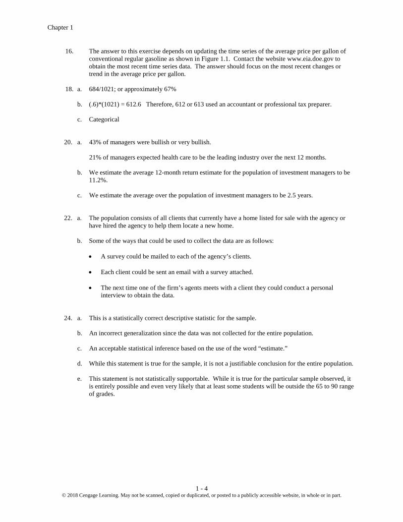
16. The answer to this exercise depends on updating the time series of the average price per gallon of conventional regular gasoline as shown in Figure 1.1. Contact the website www.eia.doe.gov to obtain the most recent time series data. The answer should focus on the most recent changes or trend in the average price per gallon.
18. a. 684/1021; or approximately 67% b. (.6)*(1021) = 612.6 Therefore, 612 or 613 used an accountant or professional tax preparer. c. Categorical 20. a. 43% of managers were bullish or very bullish. 21% of managers expected health care to be the leading industry over the next 12 months. b. We estimate the average 12-month return estimate for the population of investment managers to be
11.2%. c. We estimate the average over the population of investment managers to be 2.5 years. 22. a. The population consists of all clients that currently have a home listed for sale with the agency or
have hired the agency to help them locate a new home. b. Some of the ways that could be used to collect the data are as follows:
• A survey could be mailed to each of the agency’s clients.
• Each client could be sent an email with a survey attached.
• The next time one of the firm’s agents meets with a client they could conduct a personal interview to obtain the data.
24. a. This is a statistically correct descriptive statistic for the sample. b. An incorrect generalization since the data was not collected for the entire population. c. An acceptable statistical inference based on the use of the word “estimate.” d. While this statement is true for the sample, it is not a justifiable conclusion for the entire population. e. This statement is not statistically supportable. While it is true for the particular sample observed, it
is entirely possible and even very likely that at least some students will be outside the 65 to 90 range of grades.

2 - 1 © 2018 Cengage Learning. May not be scanned, copied or duplicated, or posted to a publicly accessible website, in whole or in part.
Chapter 2 Descriptive Statistics: Tabular and Graphical Displays Solutions: 2. a. 1 – (.22 + .18 + .40) = .20 b. .20(200) = 40 c/d.
Class Frequency Percent Frequency A .22(200) = 44 22 B .18(200) = 36 18 C .40(200) = 80 40 D .20(200) = 40 20
Total 200 100 3. a. 360° x 58/120 = 174° b. 360° x 42/120 = 126° c.
No35.0%
Yes48.3%
No Opinion16.7%

Chapter 2
2 - 2 © 2018 Cengage Learning. May not be scanned, copied or duplicated, or posted to a publicly accessible website, in whole or in part.
d.
4. a. These data are categorical. b.
Show Frequency % Frequency Jep 10 20 JJ 8 16
OWS 7 14 THM 12 24 WoF 13 26 Total 50 100
c.
0
10
20
30
40
50
60
70
Yes No No Opinion
Freq
uenc
y
Response
0
2
4
6
8
10
12
14
Jep JJ OWS THM WoF
Freq
uenc
y
Syndicated Television Show

Descriptive Statistics: Tabular and Graphical Displays
2 - 3 © 2018 Cengage Learning. May not be scanned, copied or duplicated, or posted to a publicly accessible website, in whole or in part.
d. The largest viewing audience is for Wheel of Fortune and the second largest is for Two and a Half Men.
6. a.
Network Relative
Frequency % Frequency ABC 6 24 CBS 9 36 FOX 1 4 NBC 9 36 Total: 25 100
b. For these data, NBC and CBS tie for the number of top-rated shows. Each has 9 (36%) of the top 25.
ABCis third with 6 (24%) and the much younger FOX network has 1(4%).
Jep20%
JJ16%
OWS14%
THM24%
WoF26%
Syndicated Television Shows
0123456789
10
ABC CBS FOX NBC
Freq
uenc
y
Network

Chapter 2
2 - 4 © 2018 Cengage Learning. May not be scanned, copied or duplicated, or posted to a publicly accessible website, in whole or in part.
7. a. Rating Frequency Percent Frequency Excellent 20 40 Very Good 23 46 Good 4 8 Fair 1 2 Poor 2 4 50 100
Management should be very pleased with the survey results. 40% + 46% = 86% of the ratings are
very good to excellent. 94% of the ratings are good or better. This does not look to be a Delta flight where significant changes are needed to improve the overall customer satisfaction ratings.
b. While the overall ratings look fine, note that one customer (2%) rated the overall experience with the
flight as Fair and two customers (4%) rated the overall experience with the flight as Poor. It might be insightful for the manager to review explanations from these customers as to how the flight failed to meet expectations. Perhaps, it was an experience with other passengers that Delta could do little to correct or perhaps it was an isolated incident that Delta could take steps to correct in the future.
8. a.
Position Frequency Relative Frequency Pitcher 17 0.309 Catcher 4 0.073 1st Base 5 0.091 2nd Base 4 0.073 3rd Base 2 0.036 Shortstop 5 0.091 Left Field 6 0.109 Center Field 5 0.091 Right Field 7 0.127 55 1.000
b. Pitchers (Almost 31%) c. 3rd Base (3 – 4%) d. Right Field (Almost 13%)
05
101520253035404550
Poor Fair Good Very Good Excellent
Perc
ent F
requ
ency
Customer Rating

Descriptive Statistics: Tabular and Graphical Displays
2 - 5 © 2018 Cengage Learning. May not be scanned, copied or duplicated, or posted to a publicly accessible website, in whole or in part.
e. Infielders (16 or 29.1%) to Outfielders (18 or 32.7%) 10. a.
Rating Frequency
Excellent 187 Very Good 252 Average 107 Poor 62 Terrible 41 Total 649
b.
Rating Percent
Frequency Excellent 29 Very Good 39 Average 16 Poor 10 Terrible 6 Total 100
c.
d. 29% + 39% = 68% of the guests at the Sheraton Anaheim Hotel rated the hotel as Excellent or Very
Good. But, 10% + 6% = 16% of the guests rated the hotel as poor or terrible.
e. The percent frequency distribution for Disney’s Grand Californian follows:
Rating Percent
Frequency Excellent 48 Very Good 31 Average 12 Poor 6
0
5
10
15
20
25
30
35
40
45
Excellent Very Good Average Poor Terrible
Perc
ent F
requ
ency
Rating

Chapter 2
2 - 6 © 2018 Cengage Learning. May not be scanned, copied or duplicated, or posted to a publicly accessible website, in whole or in part.
Terrible 3 Total 100
48% + 31% = 79% of the guests at the Sheraton Anaheim Hotel rated the hotel as Excellent or Very
Good. And, 6% + 3% = 9% of the guests rated the hotel as poor or terrible. Compared to ratings of other hotels in the same region, both of these hotels received very favorable
ratings. But, in comparing the two hotels, guests at Disney’s Grand Californian provided somewhat better ratings than guests at the Sheraton Anaheim Hotel.
12.
Class Cumulative Frequency Cumulative Relative Frequency less than or equal to 19 10 .20 less than or equal to 29 24 .48 less than or equal to 39 41 .82 less than or equal to 49 48 .96 less than or equal to 59 50 1.00
14. a.
b/c.
Class Frequency Percent Frequency 6.0 – 7.9 4 20 8.0 – 9.9 2 10 10.0 – 11.9 8 40 12.0 – 13.9 3 15 14.0 – 15.9 3 15
20 100 15. Leaf Unit = .1
6 3
7 5 5 7
8 1 3 4 8
9 3 6
10 0 4 5
11 3
6.0 8.0 10.0 12.0 14.0 16.0
Descriptive Statistics: Tabular and Graphical Displays
2 - 7 © 2018 Cengage Learning. May not be scanned, copied or duplicated, or posted to a publicly accessible website, in whole or in part.
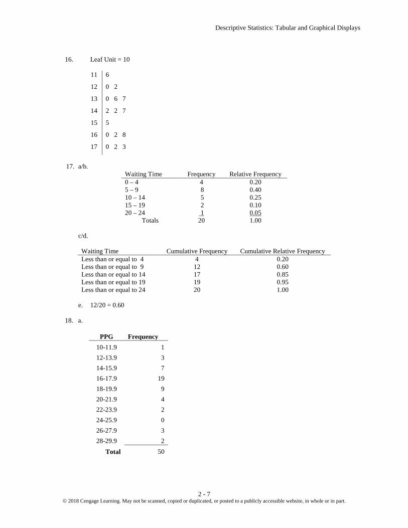
16. Leaf Unit = 10
11 6
12 0 2
13 0 6 7
14 2 2 7
15 5
16 0 2 8
17 0 2 3
17. a/b.
Waiting Time Frequency Relative Frequency 0 – 4 4 0.20 5 – 9 8 0.40 10 – 14 5 0.25 15 – 19 2 0.10 20 – 24 1 0.05
Totals 20 1.00
c/d.
Waiting Time Cumulative Frequency Cumulative Relative Frequency Less than or equal to 4 4 0.20 Less than or equal to 9 12 0.60 Less than or equal to 14 17 0.85 Less than or equal to 19 19 0.95 Less than or equal to 24 20 1.00
e. 12/20 = 0.60
18. a.
PPG Frequency 10-11.9 1 12-13.9 3 14-15.9 7 16-17.9 19 18-19.9 9 20-21.9 4 22-23.9 2 24-25.9 0 26-27.9 3 28-29.9 2
Total 50

Chapter 2
2 - 8 © 2018 Cengage Learning. May not be scanned, copied or duplicated, or posted to a publicly accessible website, in whole or in part.
b.
PPG Relative
Frequency 10-11.9 0.02 12-13.9 0.06 14-15.9 0.14 16-17.9 0.38 18-19.9 0.18 20-21.9 0.08 22-23.9 0.04 24-25.9 0.00 26-27.9 0.06 28-29.9 0.04
Total 1.00 c.
PPG
Cumulative Percent
Frequency less than 12 2 less than 14 8 less than 16 22 less than 18 60 less than 20 78 less than 22 86 less than 24 90 less than 26 90 less than 28 96 less than 30 100
d.
e. There is skewness to the right.
0
2
4
6
8
10
12
14
16
18
20
10-12 12-14 14-16 16-18 18-20 20-22 22-24 24-26 26-28 28-30
Freq
uenc
y
PPG
Descriptive Statistics: Tabular and Graphical Displays
2 - 9 © 2018 Cengage Learning. May not be scanned, copied or duplicated, or posted to a publicly accessible website, in whole or in part.
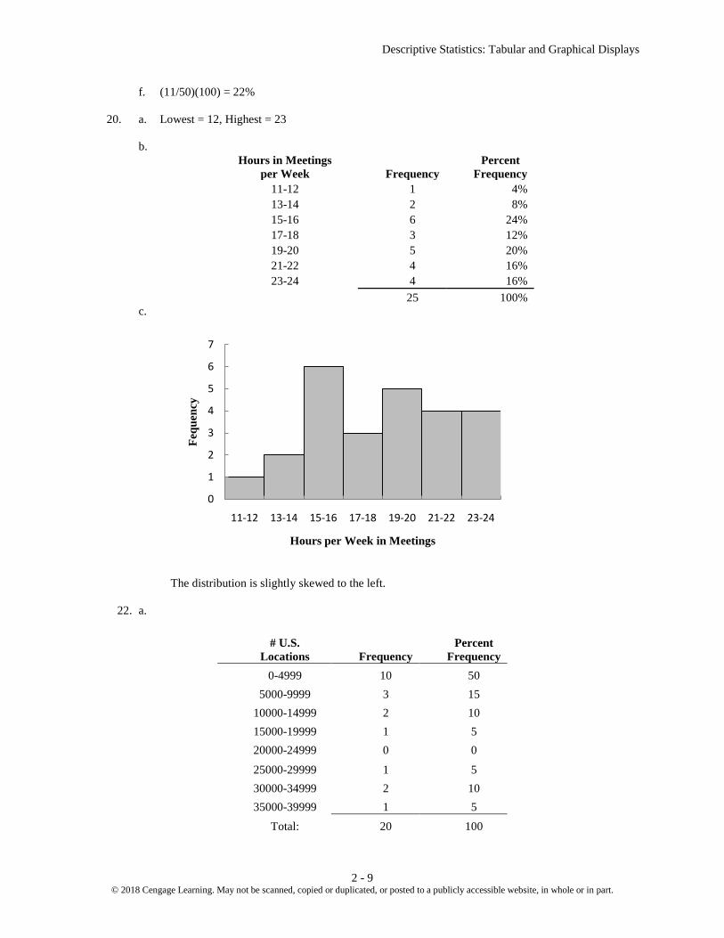
f. (11/50)(100) = 22%
20. a. Lowest = 12, Highest = 23 b.
Hours in Meetings per Week Frequency
Percent Frequency
11-12 1 4% 13-14 2 8% 15-16 6 24% 17-18 3 12% 19-20 5 20% 21-22 4 16% 23-24 4 16%
25 100%
c.
The distribution is slightly skewed to the left. 22. a.
0
1
2
3
4
5
6
7
11-12 13-14 15-16 17-18 19-20 21-22 23-24
Fequ
ency
Hours per Week in Meetings
# U.S. Locations Frequency
Percent Frequency
0-4999 10 50 5000-9999 3 15
10000-14999 2 10 15000-19999 1 5 20000-24999 0 0
25000-29999 1 5 30000-34999 2 10 35000-39999 1 5
Total: 20 100

Chapter 2
2 - 10 © 2018 Cengage Learning. May not be scanned, copied or duplicated, or posted to a publicly accessible website, in whole or in part.
b.
c. The distribution is skewed to the right. The majority of the franchises in this list have fewer than
20,000 locations (50% + 15% + 15% = 80%). McDonald's, Subway and 7-Eleven have the highestnumberof locations.
24. Leaf Unit = 1000
Starting Median Salary
4 6 8 5 1 2 3 3 5 6 8 8 6 0 1 1 1 2 2 7 1 2 5
Leaf Unit = 1000 Mid-Career Median Salary
8 0 0 4 9 3 3 5 6 7
10 5 6 6 11 0 1 4 4 4 12 2 3 6
There is a wider spread in the mid-career median salaries than in the starting median salaries. Also, as expected, the mid-career median salaries are higher that the starting median salaries. The mid-career median salaries were mostly in the $93,000 to $114,000 range while the starting median salaries were mostly in the $51,000 to $62,000 range.
0
2
4
6
8
10
12
0 -4999
5000 -9999
10000 -14999
15000 -19999
20000 -24999
25000 -29999
30000 -34999
35000 -39999
Freq
uenc
y
Number of U.S. Locations

Descriptive Statistics: Tabular and Graphical Displays
2 - 11 © 2018 Cengage Learning. May not be scanned, copied or duplicated, or posted to a publicly accessible website, in whole or in part.
26. a. 2 1 4 2 6 7 3 0 1 1 1 2 3 3 5 6 7 7 4 0 0 3 3 3 3 3 4 4 4 6 6 7 9 5 0 0 0 2 2 5 5 6 7 9 6 1 4 6 6 7 2
b. Most frequent age group: 40-44 with 9 runners c. 43 was the most frequent age with 5 runners 27. a.
y
x
A
B
C
5
11
2
0
2
10
12 18
5
13
12
30
Total 1 2
Total
b.
y
x
A
B
C
100.0
84.6
16.7
1
0.0
15.4
83.3
2
100.0
100.0
100.0
Total
c.
Chapter 2
2 - 12 © 2018 Cengage Learning. May not be scanned, copied or duplicated, or posted to a publicly accessible website, in whole or in part.
y
x
A
B
C
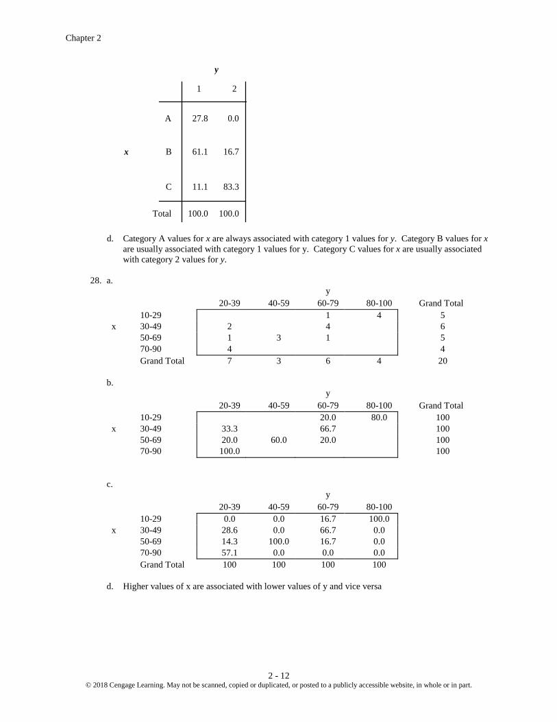
27.8
61.1
11.1
100.0
0.0
16.7
83.3
100.0
1 2
Total
d. Category A values for x are always associated with category 1 values for y. Category B values for x
are usually associated with category 1 values for y. Category C values for x are usually associated with category 2 values for y.
28. a.
y 20-39 40-59 60-79 80-100 Grand Total 10-29 1 4 5
x 30-49 2 4 6 50-69 1 3 1 5 70-90 4 4 Grand Total 7 3 6 4 20
b.
y 20-39 40-59 60-79 80-100 Grand Total 10-29 20.0 80.0 100
x 30-49 33.3 66.7 100 50-69 20.0 60.0 20.0 100 70-90 100.0 100
c.
y 20-39 40-59 60-79 80-100 10-29 0.0 0.0 16.7 100.0
x 30-49 28.6 0.0 66.7 0.0 50-69 14.3 100.0 16.7 0.0 70-90 57.1 0.0 0.0 0.0 Grand Total 100 100 100 100
d. Higher values of x are associated with lower values of y and vice versa

Descriptive Statistics: Tabular and Graphical Displays
2 - 13 © 2018 Cengage Learning. May not be scanned, copied or duplicated, or posted to a publicly accessible website, in whole or in part.
30. a. Row Percentages
Year
Average Speed 1988-1992 1993-1997 1998-2002 2003-2007 2008-2012 Total 130-139.9 16.7 0.0 0.0 33.3 50.0 100 140-149.9 25.0 25.0 12.5 25.0 12.5 100 150-159.9 0.0 50.0 16.7 16.7 16.7 100 160-169.9 50.0 0.0 50.0 0.0 0.0 100 170-179.9 0.0 0.0 100.0 0.0 0.0 100
b. It appears that most of the faster average winning times occur before 2003. This could be due to new
regulations that take into account driver safety, fan safety, the environmental impact, and fuel consumption during races.
32. a. Row percentages are shown below.
Region Under
$15,000
$15,000 to
$24,999
$25,000 to
$34,999
$35,000 to
$49,999
$50,000 to
$74,999
$75,000 to
$99,999 $100,000 and over Total
Northeast 12.72 10.45 10.54 13.07 17.22 11.57 24.42 100.00 Midwest 12.40 12.60 11.58 14.27 19.11 12.06 17.97 100.00 South 14.30 12.97 11.55 14.85 17.73 11.04 17.57 100.00 West 11.84 10.73 10.15 13.65 18.44 11.77 23.43 100.00
The percent frequency distributions for each region now appear in each row of the table. For example, the percent frequency distribution of the West region is as follows:
Income Level Percent
Frequency Under $15,000 11.84 $15,000 to $24,999 10.73 $25,000 to $34,999 10.15 $35,000 to $49,999 13.65 $50,000 to $74,999 18.44 $75,000 to $99,999 11.77 $100,000 and over 23.43
Total 100.00
b. West: 18.44 + 11.77 + 23.43 = 53.64%or (4804 + 3066 + 6104) / 26057 = 53.63% South: 17.73 + 11.04 + 17.57 = 46.34%or (7730 + 4813 + 7660) / 43609 = 46.33%
c.

Chapter 2
2 - 14 © 2018 Cengage Learning. May not be scanned, copied or duplicated, or posted to a publicly accessible website, in whole or in part.
0.00
5.00
10.00
15.00
20.00
25.00
Under $15,000
$15,000 to $24,999
$25,000 to $34,999
$35,000 to $49,999
$50,000 to $74,999
$75,000 to $99,999
$100,000 and over
Perc
ent F
requ
ency
Income Level
Northeast
0.00
5.00
10.00
15.00
20.00
25.00
Under $15,000
$15,000 to $24,999
$25,000 to $34,999
$35,000 to $49,999
$50,000 to $74,999
$75,000 to $99,999
$100,000 and over
Perc
ent F
requ
ency
Income Level
Midwest
0.00
5.00
10.00
15.00
20.00
25.00
Under $15,000
$15,000 to $24,999
$25,000 to $34,999
$35,000 to $49,999
$50,000 to $74,999
$75,000 to $99,999
$100,000 and over
Perc
ent F
requ
ency
Income Level
South
Descriptive Statistics: Tabular and Graphical Displays
2 - 15 © 2018 Cengage Learning. May not be scanned, copied or duplicated, or posted to a publicly accessible website, in whole or in part.
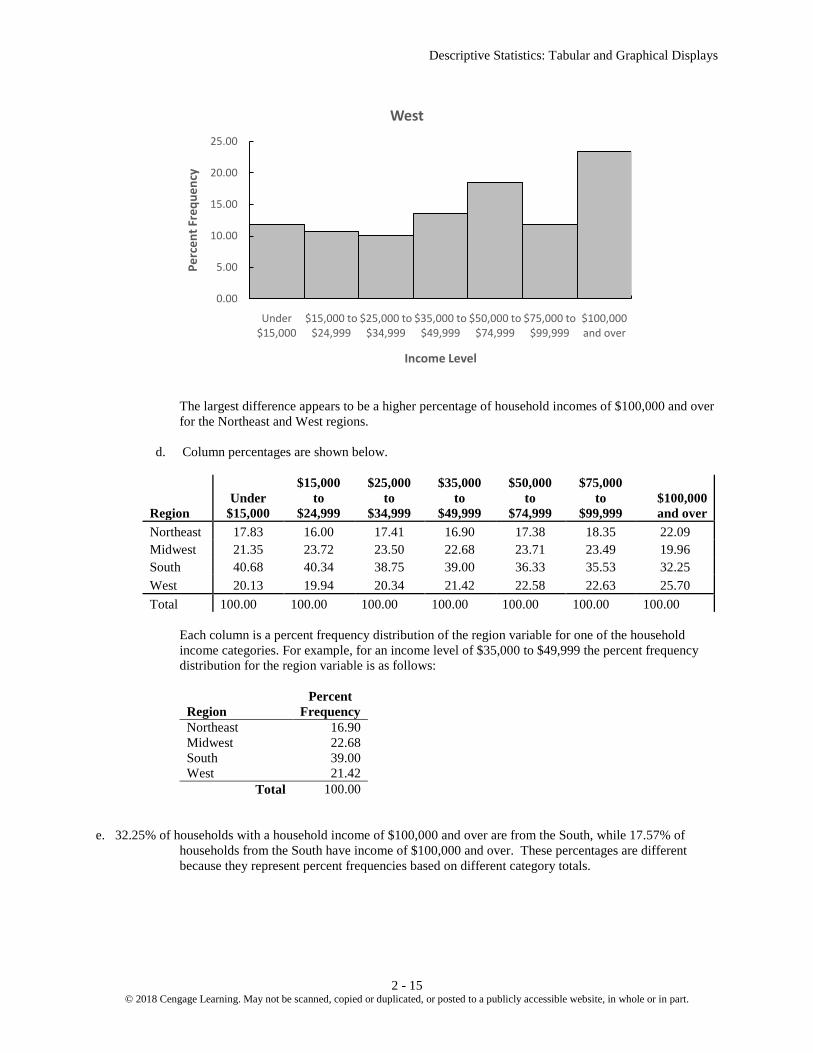
The largest difference appears to be a higher percentage of household incomes of $100,000 and over for the Northeast and West regions.
d. Column percentages are shown below.
Region Under
$15,000
$15,000 to
$24,999
$25,000 to
$34,999
$35,000 to
$49,999
$50,000 to
$74,999
$75,000 to
$99,999 $100,000 and over
Northeast 17.83 16.00 17.41 16.90 17.38 18.35 22.09 Midwest 21.35 23.72 23.50 22.68 23.71 23.49 19.96 South 40.68 40.34 38.75 39.00 36.33 35.53 32.25 West 20.13 19.94 20.34 21.42 22.58 22.63 25.70 Total 100.00 100.00 100.00 100.00 100.00 100.00 100.00
Each column is a percent frequency distribution of the region variable for one of the household
income categories. For example, for an income level of $35,000 to $49,999 the percent frequency distribution for the region variable is as follows:
Region
Percent Frequency
Northeast 16.90 Midwest 22.68 South 39.00 West 21.42
Total 100.00
e. 32.25% of households with a household income of $100,000 and over are from the South, while 17.57% of households from the South have income of $100,000 and over. These percentages are different because they represent percent frequencies based on different category totals.
0.00
5.00
10.00
15.00
20.00
25.00
Under $15,000
$15,000 to $24,999
$25,000 to $34,999
$35,000 to $49,999
$50,000 to $74,999
$75,000 to $99,999
$100,000 and over
Perc
ent F
requ
ency
Income Level
West

Chapter 2
2 - 16 © 2018 Cengage Learning. May not be scanned, copied or duplicated, or posted to a publicly accessible website, in whole or in part.
34. a.
Brand Revenue ($ billions)
Industry 0-25 25-50 50-75 75-100 100-125 125-150 Total Automotive & Luxury 10 1 1
1 2 15
Consumer Packaged Goods 12
12 Financial Services 2 4 2 2 2 2 14 Other 13 5 3 2 2 1 26 Technology 4 4 4 1 2
15
Total 41 14 10 5 7 5 82 b.
Brand Revenue ($ billions) Frequency 0-25 41 25-50 14 50-75 10
75-100 5 100-125 7 125-150 5
Total 82 c. Consumer packaged goods have the lowest brand revenues; each of the 12 consumer packaged
goods brands in the sample data had a brand revenue of less than $25 billion. Approximately 57% of the financial services brands (8 out of 14) had a brand revenue of $50 billion or greater, and 47% of the technology brands (7 out of 15) had a brand revenue of at least $50 billion.
d.
1-Yr Value Change (%)
Industry -60--41 -40--21 -20--1 0-19 20-39 40-60 Total Automotive & Luxury 11 4 15 Consumer Packaged Goods 2 10 12 Financial Services 1 6 7 14 Other 2 20 4 26 Technology 1 3 4 4 2 1 15
Total 1 4 14 52 10 1 82
e.
1-Yr Value Change (%) Frequency -60--41 1 -40--21 4 -20--1 14

Descriptive Statistics: Tabular and Graphical Displays
2 - 17 © 2018 Cengage Learning. May not be scanned, copied or duplicated, or posted to a publicly accessible website, in whole or in part.
0-19 52 20-39 10 40-60 1
Total 82 f. The automotive & luxury brands all had a positive 1-year value change (%). The technology brands
had the greatest variability.Financial services were heavily concentrated between -20 and +19 % changes, while consumer goods and other industries were mostly concentrated in 0-19% gains.
36. a.
b. There is a negative relationship between x and y; y decreases as x increases. 38. a.
y
Yes No
Low 66.667 33.333 100
x Medium 30.000 70.000 100
High 80.000 20.000 100
b.
-40
-24
-8
8
24
40
56
-40 -30 -20 -10 0 10 20 30 40
y
x

Chapter 2
2 - 18 © 2018 Cengage Learning. May not be scanned, copied or duplicated, or posted to a publicly accessible website, in whole or in part.
40. a.
b. Colder average low temperature seems to lead to higher amounts of snowfall. c. Two cities have an average snowfall of nearly 100 inches of snowfall: Buffalo, N.Y and Rochester,
NY. Both are located near large lakes in New York.
0%10%20%30%40%50%60%70%80%90%
100%
Low Medium High
x
No
Yes
0
20
40
60
80
100
120
30 40 50 60 70 80
Avg
. Sno
wfa
ll (in
ches
)
Avg. Low Temp

Descriptive Statistics: Tabular and Graphical Displays
2 - 19 © 2018 Cengage Learning. May not be scanned, copied or duplicated, or posted to a publicly accessible website, in whole or in part.
42. a.
b. After an increase in age 25-34, smartphone ownership decreases as age increases. The percentage of
people with no cell phone increases with age. There is less variation across age groups in the percentage who own other cell phones.
c. Unless a newer device replaces the smartphone, we would expect smartphone ownership would
become less sensitive to age. This would be true because current users will become older and because the device will become to be seen more as a necessity than a luxury.
44. a.
0%10%20%30%40%50%60%70%80%90%
100%
18-24 25-34 35-44 45-54 55-64 65+
Age
No Cell Phone
Other Cell Phone
Smartphone
Class Frequency 800-999 1
1000-1199 3 1200-1399 6 1400-1599 10 1600-1799 7 1800-1999 2 2000-2199 1
Total 30

Chapter 2
2 - 20 © 2018 Cengage Learning. May not be scanned, copied or duplicated, or posted to a publicly accessible website, in whole or in part.
b. The distribution if nearly symmetrical. It could be approximated by a bell-shaped curve. c. 10 of 30 or 33% of the scores are between 1400 and 1599. The average SAT score looks to be a
little over 1500. Scores below 800 or above 2200 are unusual.
46. a. Population in Millions Frequency % Frequency
0.0 - 2.4 15 30.0% 2.5-4.9 13 26.0% 5.0-7.4 10 20.0% 7.5-9.9 5 10.0%
10.0-12.4 1 2.0% 12.5-14.9 2 4.0% 15.0-17.4 0 0.0% 17.5-19.9 2 4.0% 20.0-22.4 0 0.0% 22.5-24.9 0 0.0% 25.0-27.4 1 2.0% 27.5-29.9 0 0.0% 30.0-32.4 0 0.0% 32.5-34.9 0 0.0% 35.0-37.4 1 2.0% 37.5-39.9 0 0.0%
0
2
4
6
8
10
12
800-999 1000-1199 1200-1399 1400-1599 1600-1799 1800-1999 2000-2199
Freq
uenc
y
SAT Score

Descriptive Statistics: Tabular and Graphical Displays
2 - 21 © 2018 Cengage Learning. May not be scanned, copied or duplicated, or posted to a publicly accessible website, in whole or in part.
b. The distribution is skewed to the right. c. 15 states (30%) have a population less than 2.5 million. Over half of the states have population less
than 5 million (28 states – 56%). Only seven states have a population greater than 10 million (California, Florida, Illinois, New York, Ohio, Pennsylvania and Texas). The largest state is California (37.3 million) and the smallest states are Vermont and Wyoming (600 thousand).
48. a.
Industry Frequency % Frequency Bank 26 13% Cable 44 22% Car 42 21% Cell 60 30% Collection 28 14% Total 200 100%
b.
0
2
4
6
8
10
12
14
16
0.0 -2.4
2.5-4.9
5.0-7.4
7.5-9.9
10.0-12.4
12.5-14.9
15.0-17.4
17.5-19.9
20.0-22.4
22.5-24.9
25.0-27.4
27.5-29.9
30.0-32.4
32.5-34.9
35.0-37.4
37.5-39.9
Freq
uenc
y
Population Millions

Chapter 2
2 - 22 © 2018 Cengage Learning. May not be scanned, copied or duplicated, or posted to a publicly accessible website, in whole or in part.
c. The cellular phone providers had the highest number of complaints. d. The percentage frequency distribution shows that the two financial industries (banks and collection
agencies) had about the same number of complaints. Also, new car dealers and cable and satellite television companiesalso had about the same number of complaints.
50.a.
Level of Education Percent Frequency High School graduate 32,773/65,644(100) = 49.93 Bachelor's degree 22,131/65,644(100) = 33.71 Master's degree 9003/65,644(100) = 13.71 Doctoral degree 1737/65,644(100) = 2.65
Total 100.00 13.71 + 2.65 = 16.36% of heads of households have a master’s or doctoral degree. b.
Household Income Percent Frequency Under $25,000 13,128/65,644(100) = 20.00 $25,000 to $49,999 15,499/65,644(100) = 23.61 $50,000 to $99,999 20,548/65,644(100) = 31.30 $100,000 and over 16,469/65,644(100) = 25.09
Total 100.00
31.30 + 25.09 = 56.39% of households have an income of $50,000 or more. c.
Household Income
Level of Education Under
$25,000 $25,000 to
$49,999 $50,000 to
$99,999 $100,000 and
over
0%
5%
10%
15%
20%
25%
30%
35%
Bank Cable Car Cell Collection
Perc
ent F
requ
ency
Industry
Descriptive Statistics: Tabular and Graphical Displays
2 - 23 © 2018 Cengage Learning. May not be scanned, copied or duplicated, or posted to a publicly accessible website, in whole or in part.
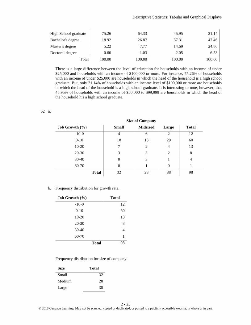
High School graduate 75.26 64.33 45.95 21.14 Bachelor's degree 18.92 26.87 37.31 47.46 Master's degree 5.22 7.77 14.69 24.86 Doctoral degree 0.60 1.03 2.05 6.53
Total 100.00 100.00 100.00 100.00
There is a large difference between the level of education for households with an income of under $25,000 and households with an income of $100,000 or more. For instance, 75.26% of households with an income of under $25,000 are households in which the head of the household is a high school graduate. But, only 21.14% of households with an income level of $100,000 or more are households in which the head of the household is a high school graduate. It is interesting to note, however, that 45.95% of households with an income of $50,000 to $99,999 are households in which the head of the household his a high school graduate.
52 a.
Size of Company Job Growth (%) Small Midsized Large Total
-10-0 4 6 2 12 0-10 18 13 29 60
10-20 7 2 4 13 20-30 3 3 2 8 30-40 0 3 1 4 60-70 0 1 0 1
Total 32 28 38 98
b. Frequency distribution for growth rate.
Job Growth (%) Total -10-0 12 0-10 60
10-20 13 20-30 8 30-40 4 60-70 1
Total 98
Frequency distribution for size of company.
Size Total Small 32 Medium 28 Large 38

Chapter 2
2 - 24 © 2018 Cengage Learning. May not be scanned, copied or duplicated, or posted to a publicly accessible website, in whole or in part.
Total 98
c. Crosstabulation showing column percentages.
Size of Company Job Growth (%) Small Midsized Large
-10-0 13 21 5 0-10 56 46 76
10-20 22 7 11 20-30 9 11 5 30-40 0 11 3 60-70 0 4 0
Total 100 100 100
d. Crosstabulation showing row percentages.
Size of Company Job Growth (%) Small Midsized Large Total
-10-0 33 50 17 100 0-10 30 22 48 100
10-20 54 15 31 100 20-30 38 38 25 100 30-40 0 75 25 100 60-70 0 100 0 100
e. 12 companies had a negative job growth: 13% were small companies; 21% were midsized companies; and 5% were large companies. So, in terms of avoiding negative job growth, large companies were better off than small and midsized companies. But, although 95% of the large companies had a positive job growth, the growth rate was below 10% for 76% of these companies. In terms of better job growth rates, midsized companies performed better than either small or large companies. For instance, 26% of the midsized companies had a job growth of at least 20% as compared to 9% for small companies and 8% for large companies.
54. a.
% Graduate Year Founded
35-40
40-45
45-50
50-55
55-60
60-65
65-70
70-75
75-80
80-85
85-90
90-95
95-100
Grand Total
1600-1649 1 1 1700-1749
3 3
1750-1799
1 3 4 1800-1849
1 2 4 2 3 4 3 2 21
1850-1899
1 2 4 3 11 5 9 6 3 4 1 49 1900-1949 1 1 1
1 3
3 2 4 1 1
18
1950-2000 1 1 3 2 7 Grand Total 2 1 3 5 5 7 15 12 13 13 8 9 10 103

Descriptive Statistics: Tabular and Graphical Displays
2 - 25 © 2018 Cengage Learning. May not be scanned, copied or duplicated, or posted to a publicly accessible website, in whole or in part.
b.
c. Older colleges and universities tend to have higher graduation rates.
56. a.
b. There appears to be a strong positive relationship between Tuition & Fees and % Graduation. 58. a.
0.00
20.00
40.00
60.00
80.00
100.00
120.00
0 10,000 20,000 30,000 40,000 50,000
% G
radu
ate
Tuition & Fees ($)
320000325000330000335000340000345000350000355000
2008 2009 2010 2011
Att
enda
nce
Year

Chapter 2
2 - 26 © 2018 Cengage Learning. May not be scanned, copied or duplicated, or posted to a publicly accessible website, in whole or in part.
Zoo attendance appears to be dropping over time. b.
c. General attendance is increasing, but not enough to offset the decrease in member attendance.
School membership appears fairly stable.
0
20,000
40,000
60,000
80,000
100,000
120,000
140,000
160,000
180,000
2008 2009 2010 2011
Att
enda
nce
Year
General
Member
School

3 - 1 © 2018 Cengage Learning. May not be scanned, copied or duplicated, or posted to a publicly accessible website, in whole or in part.
Chapter 3 Descriptive Statistics: Numerical Measures Solutions:
2. x xn
i= = =Σ 96
616
10, 12, 16, 17, 20, 21
Median = 16 17 16.52+
=
3. a. x w xwi i
i
= =+ + +
+ + += =
ΣΣ
6 32 3 2 2 2 5 8 56 3 2 8
70 219
369( . ) ( ) ( . ) ( ) . .
b. 32 2 2 5 54
12 74
3175. . . .+ + += =
4.
Period Rate of Return (%) 1 -6.0 2 -8.0 3 -4.0 4 2.0 5 5.4
The mean growth factor over the five periods is:
( )( ) ( ) ( )( )( )( )( ) 55
1 2 5 0.940 0.920 0.960 1.020 1.054 0.8925 0.9775ngx x x x= = = =
So the mean growth rate (0.9775 – 1)100% = –2.25%. 5. 15, 20, 25, 25, 27, 28, 30, 34
2020( 1) (8 1) 1.8
100 100pL n= + = + =
20th percentile = 15 + .8(20 – 15) = 19
2525( 1) (8 1) 2.25
100 100pL n= + = + =
25th percentile = 20 + .25(25 – 20) = 21.25
Chapter 3
3 - 2 © 2018 Cengage Learning.May not be scanned, copied or duplicated, or posted to a publicly accessible website, in whole or in part.
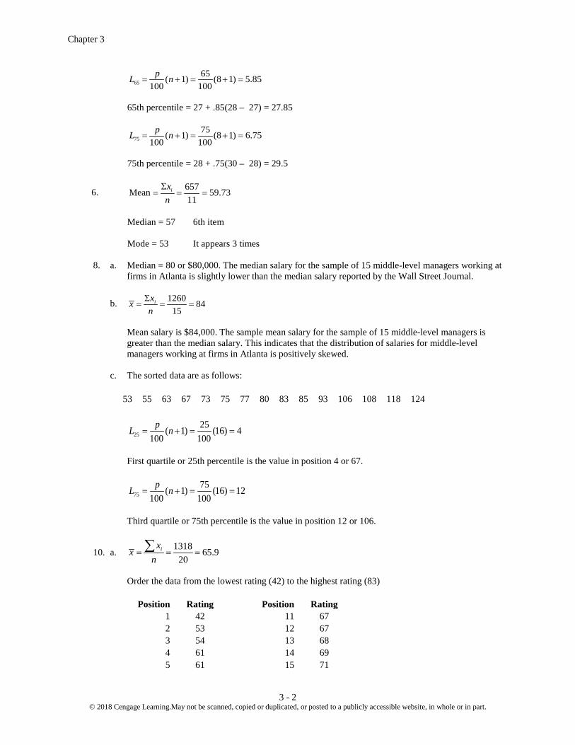
6565( 1) (8 1) 5.85
100 100pL n= + = + =
65th percentile = 27 + .85(28 – 27) = 27.85
7575( 1) (8 1) 6.75
100 100pL n= + = + =
75th percentile = 28 + .75(30 – 28) = 29.5
6. 657Mean 59.7311
ixnΣ
= = =
Median = 57 6th item Mode = 53 It appears 3 times 8. a. Median = 80 or $80,000. The median salary for the sample of 15 middle-level managers working at
firms in Atlanta is slightly lower than the median salary reported by the Wall Street Journal.
b. 1260 8415
ixxnΣ
= = =
Mean salary is $84,000. The sample mean salary for the sample of 15 middle-level managers is
greater than the median salary. This indicates that the distribution of salaries for middle-level managers working at firms in Atlanta is positively skewed.
c. The sorted data are as follows:
53 55 63 67 73 75 77 80 83 85 93 106 108 118 124
2525( 1) (16) 4
100 100pL n= + = =
First quartile or 25th percentile is the value in position 4 or 67.
7575( 1) (16) 12
100 100pL n= + = =
Third quartile or 75th percentile is the value in position 12 or 106.
10. a. 1318 65.920
ixx
n= = =∑
Order the data from the lowest rating (42) to the highest rating (83)
Position Rating
Position Rating 1 42
11 67
2 53
12 67 3 54
13 68
4 61
14 69 5 61
15 71

Descriptive Statistics: Numerical Measures
3 - 3 © 2018 Cengage Learning. May not be scanned, copied or duplicated, or posted to a publicly accessible website, in whole or in part.
6 61
16 71 7 62
17 76
8 63
18 78 9 64
19 81
10 66
20 83
5050( 1) (20 1) 10.5
100 100pL n= + = + =
Median or 50th percentile = 66 + . 5(67 – 66) = 66.5 Mode is 61.
b. 2525( 1) (20 1) 5.25
100 100pL n= + = + =
First quartile or 25th percentile = 61
7575( 1) (20 1) 15.75
100 100pL n= + = + =
Third quartile or 75th percentile = 71
c. 9090( 1) (20 1) 18.9
100 100pL n= + = + =
90th percentile = 78 + .9(81 – 78) = 80.7 90% of the ratings are 80.7 or less;10% of the ratings are 80.7 or greater. 12. a. The minimum number of viewers that watched a new episode is 13.3 million, and the maximum
number is 16.5 million. b. The mean number of viewers that watched a new episode is 15.04 million or approximately
15.0 million; the median also 15.0 million. The data is multimodal (13.6, 14.0, 16.1, and 16.2 million); in such cases the mode is usually not reported.
c. The data are first arranged in ascending order.
2525( 1) (21 1) 5.50
100 100pL n= + = + =
First quartile or 25th percentile = 14 + .50(14.1 – 14) = 14.05
7575( 1) (21 1) 16.5
100 100pL n= + = + =
Third quartile or 75th percentile = 16 + . 5(16.1 – 16) = 16.05 d. A graph showing the viewership data over the air dates follows. Period 1 corresponds to the first
episode of the season, period 2 corresponds to the second episode, and so on.
Chapter 3
3 - 4 © 2018 Cengage Learning.May not be scanned, copied or duplicated, or posted to a publicly accessible website, in whole or in part.
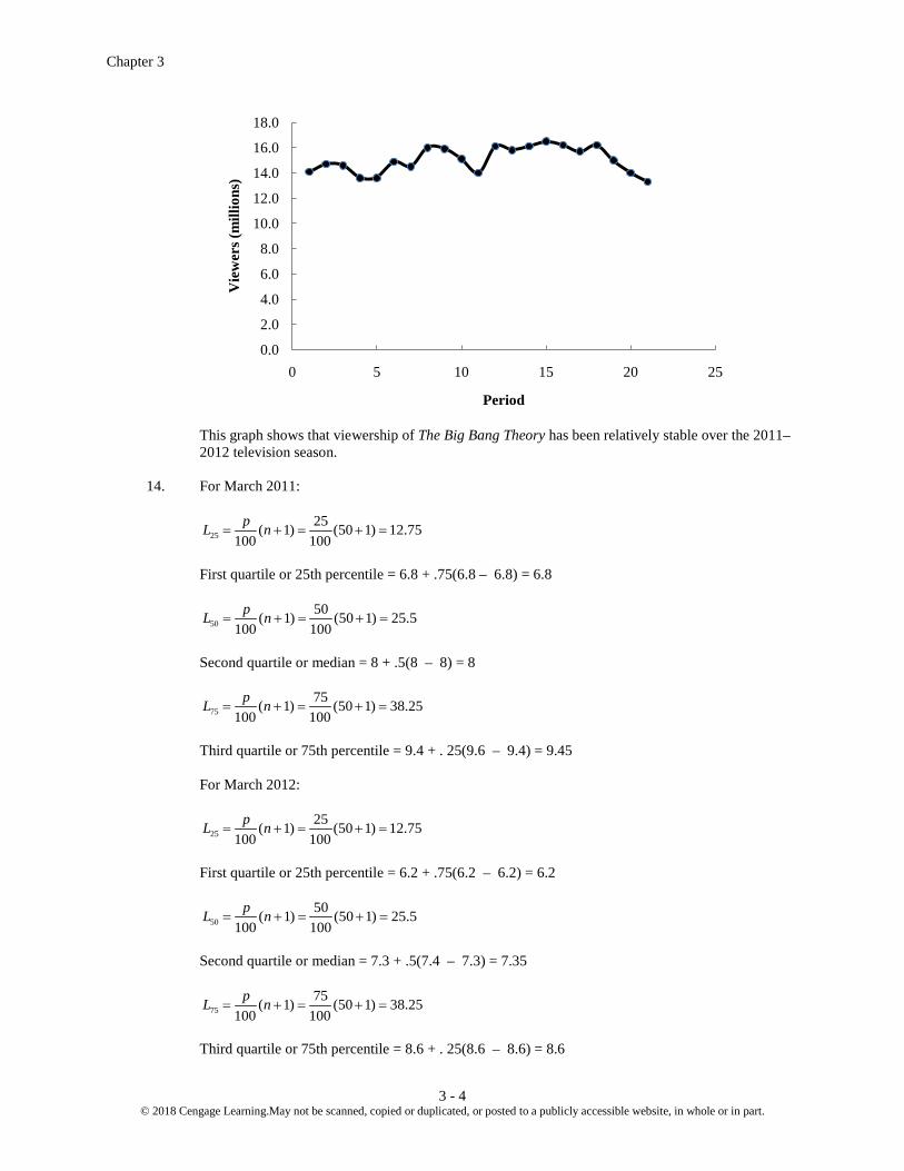
This graph shows that viewership of The Big Bang Theory has been relatively stable over the 2011–
2012 television season. 14. For March 2011:
2525( 1) (50 1) 12.75
100 100pL n= + = + =
First quartile or 25th percentile = 6.8 + .75(6.8 – 6.8) = 6.8
5050( 1) (50 1) 25.5
100 100pL n= + = + =
Second quartile or median = 8 + .5(8 – 8) = 8
7575( 1) (50 1) 38.25
100 100pL n= + = + =
Third quartile or 75th percentile = 9.4 + . 25(9.6 – 9.4) = 9.45 For March 2012:
2525( 1) (50 1) 12.75
100 100pL n= + = + =
First quartile or 25th percentile = 6.2 + .75(6.2 – 6.2) = 6.2
5050( 1) (50 1) 25.5
100 100pL n= + = + =
Second quartile or median = 7.3 + .5(7.4 – 7.3) = 7.35
7575( 1) (50 1) 38.25
100 100pL n= + = + =
Third quartile or 75th percentile = 8.6 + . 25(8.6 – 8.6) = 8.6
0.0
2.0
4.0
6.0
8.0
10.0
12.0
14.0
16.0
18.0
0 5 10 15 20 25
Vie
wer
s (m
illio
ns)
Period

Descriptive Statistics: Numerical Measures
3 - 5 © 2018 Cengage Learning. May not be scanned, copied or duplicated, or posted to a publicly accessible website, in whole or in part.
It may be easier to compare these results if we place them in a table.
March 2011 March 2012 First Quartile 6.80 6.20 Median 8.00 7.35 Third Quartile 9.45 8.60
The results show that in March 2012 approximately 25% of the states had an unemployment rate of
6.2% or less, lower than in March 2011. And, the median of 7.35% and the third quartile of 8.6% in March 2012 are both less than the corresponding values in March 2011, indicating that unemployment rates across the states are decreasing.
16. a.
Grade xi Weight wi
4 (A) 9 3 (B) 15 2 (C) 33 1 (D) 3 0 (F) 0
60 Credit Hours
9(4) 15(3) 33(2) 3(1) 150 2.509 15 33 3 60
i i
i
w xx
w+ + +
= = = =+ + +
∑∑
b. Yes; satisfies the 2.5 grade point average requirement 18.
Assessment Deans wixi Recruiters wixi 5 44 220 31 155 4 66 264 34 136 3 60 180 43 129 2 10 20 12 24 1 0 0 0 0
Total 180 684 120 444
Deans: 684 3.8180
i i
i
w xx
w= = =∑∑
Recruiters: 444 3.7120
i i
i
w xx
w= = =∑∑
Business school deans rated the overall academic quality of master’s programs slightly higher than corporate recruiters did. 20.
Stivers Trippi
Year End of Year
Value Growth Factor
End of Year Value
Growth Factor
Year1 $11,000 1.100 $5,600 1.120

Chapter 3
3 - 6 © 2018 Cengage Learning.May not be scanned, copied or duplicated, or posted to a publicly accessible website, in whole or in part.
Year 2 $12,000 1.091 $6,300 1.125 Year 3 $13,000 1.083 $6,900 1.095 Year 4 $14,000 1.077 $7,600 1.101 Year 5 $15,000 1.071 $8,500 1.118 Year 6 $16,000 1.067 $9,200 1.082 Year 7 $17,000 1.063 $9,900 1.076 Year 8 $18,000 1.059 $10,600 1.071
For the Stivers mutual fund we have: 18000=10000 ( )( ) ( )1 2 8x x x , so ( )( ) ( )1 2 8x x x =1.8 and
( )( ) ( ) 81 2 8 1.80 1.07624n
gx x x x= = = So the mean annual return for the Stivers mutual fund is (1.07624 – 1)100 = 7.624% For the Trippi mutual fund we have: 10600=5000 ( )( ) ( )1 2 8x x x , so ( )( ) ( )1 2 8x x x =2.12 and ( )( ) ( ) 8
1 2 8 2.12 1.09848ngx x x x= = =
So the mean annual return for the Trippi mutual fund is (1.09848 – 1)100 = 9.848%. While the Stivers mutual fund has generated a nice annual return of 7.6%, the annual return of 9.8%
earned by the Trippi mutual fund is far superior. 22. 25,000,000=10,000,000 ( )( ) ( )1 2 6x x x , so ( )( ) ( )1 2 6x x x =2.50, and so ( )( ) ( ) 6
1 2 6 2.50 1.165ngx x x x= = =
So the mean annual growth rate is (1.165 – 1)100 = 16.5%
24. x xn
i= = =Σ 75
515
s x xn
i22
1644
16=−−
= =Σ( )
s = =16 4 25. 15, 20, 25, 25, 27, 28, 30, 34 Range = 34 – 15 = 19
2525( 1) (9) 2.25
100 100pL n= + = =
First Quartile or Q1 = 20 + .25(25-20) = 21.25

Descriptive Statistics: Numerical Measures
3 - 7 © 2018 Cengage Learning. May not be scanned, copied or duplicated, or posted to a publicly accessible website, in whole or in part.
7575( 1) (9) 6.75
100 100pL n= + = =
Third Quartile or Q3 = 28 + .75(30-28) = 29.5 IQR = Q3–Q1 = 29.5– 21.25 = 8.25
x xn
i= = =Σ 204
8255.
s x xn
i22
1242
734 57=
−−
= =Σ( )
.
s = =34 57 588. .
26. a. 74.4 3.7220
iix
xn
= = =∑
b. 2( ) 1.6516 .0869 .2948
1 20 1ii
x xs
n−
= = = =− −
∑
c. The average price for a gallon of unleaded gasoline in San Francisco is much higher than the
national average. This indicates that the cost of living in San Francisco is higher than it would be for cities that have an average price close to the national average.
28. a. The mean serve speed is 180.95, the variance is 21.42, and the standard deviation is 4.63. b. Although the mean serve speed for the twenty Women's Singles serve speed leaders for the 2011
Wimbledon tournament is slightly higher, the difference is very small. Furthermore,given the variation in the twenty Women's Singles serve speed leaders from the 2012 Australian Open and the twenty Women's Singles serve speed leaders from the 2011 Wimbledon tournament, the difference in the mean serve speeds is most likely due to random variation in the players’ performances.
30. Dawson Supply: Range = 11 – 9 = 2
4.1 0.679
s = =
J.C. Clark: Range = 15 – 7 = 8
60.1 2.58
9s = =
32. a. Automotive: 39201 1960.0520
ixx
n= = =∑
Department store: 13857 692.8520
ixx
n= = =∑

Chapter 3
3 - 8 © 2018 Cengage Learning.May not be scanned, copied or duplicated, or posted to a publicly accessible website, in whole or in part.
b. Automotive: 2( ) 4, 407,720.95 481.65
( 1) 19ix x
sn−
= = =−
∑
Department store: 2( ) 456804.55 155.06
( 1) 19ix x
sn−
= = =−
∑
c. Automotive: 2901 – 598 = 2303 Department Store: 1011 – 448 = 563 d. Order the data for each variable from the lowest to highest.
Automotive Department Store
1 598 448 2 1512 472 3 1573 474 4 1642 573 5 1714 589 6 1720 597 7 1781 598 8 1798 622 9 1813 629
10 2008 669 11 2014 706 12 2024 714 13 2058 746 14 2166 760 15 2202 782 16 2254 824 17 2366 840 18 2526 856 19 2531 947 20 2901 1011
2525( 1) (21) 5.25
100 100pL n= + = =
Automotive: First quartile or 25th percentile = 1714 + .25(1720 – 1714) = 1715.5 Department Store: First quartile or 25th percentile = 589 + .25(597 – 589) = 591
7575( 1) (21) 15.75
100 100pL n= + = =
Automotive: Third quartile or 75th percentile = 2202 + .75(2254 – 2202) = 2241 Department Store: First quartile or 75th percentile = 782 + .75(824 – 782) = 813.5 Automotive IQR = Q3 –Q1 = 2241 - 1715.5 = 525.5 Department Store IQR = Q3 –Q1 = 813.5 - 591 = 222.5

Descriptive Statistics: Numerical Measures
3 - 9 © 2018 Cengage Learning. May not be scanned, copied or duplicated, or posted to a publicly accessible website, in whole or in part.
e. Automotive spends more on average, has a larger standard deviation, larger max and min, and larger range than Department Store. Autos have all new model years and may spend more heavily on advertising.
34. Quarter milers s = 0.0564 Coefficient of Variation = (s/ x )100% = (0.0564/0.966)100% = 5.8% Milers s = 0.1295 Coefficient of Variation = (s/ x )100% = (0.1295/4.534)100% = 2.9% Yes; the coefficient of variation shows that as a percentage of the mean the quarter milers’ times
show more variability.
36. 520 500 .20100
z −= = +
650 500 1.50100
z −= = +
500 500 0.00100
z −= =
450 500 .50100
z −= = −
280 500 2.20100
z −= = −
37. a. 20 30 40 302, 25 5
z z− −= = − = = 2
11 .752
− = At least 75%
b. 15 30 45 303, 35 5
z z− −= = − = = 2
11 .893
− = At least 89%
c. 22 30 38 301.6, 1.65 5
z z− −= = − = = 2
11 .611.6
− = At least 61%
d. 18 30 42 302.4, 2.45 5
z z− −= = − = = 2
11 .832.4
− = At least 83%
e. 12 30 48 303.6, 3.65 5
z z− −= = − = = 2
11 .923.6
− = At least 92%
38. a. Approximately 95% b. Almost all c. Approximately 68%

Chapter 3
3 - 10 © 2018 Cengage Learning.May not be scanned, copied or duplicated, or posted to a publicly accessible website, in whole or in part.
39. a. This is from 2 standard deviations below the mean to 2 standard deviations above the mean. With z = 2, Chebyshev’s theorem gives:
1 1 1 12
1 14
342 2− = − = − =
z = .75
Therefore, at least 75% of adults sleep between 4.5 and 9.3 hours per day. b. This is from 2.5 standard deviations below the mean to 2.5 standard deviations above the mean. With z = 2.5, Chebyshev’s theorem gives:
2 2
1 1 11 1 1 .846.252.5z
− = − = − =
Therefore, at least 84% of adults sleep between 3.9 and 9.9 hours per day. c. With z = 2, the empirical rule suggests that 95% of adults sleep between 4.5and 9.3 hours per day.
The percentage obtained using the empirical rule is greater than the percentage obtained using Chebyshev’s theorem.
40. a. $3.33 is one standard deviation below the mean and $3.53 is one standard deviation above the mean.
The empirical rule says that approximately 68% of gasoline sales are in this price range. b. Part (a) shows that approximately 68% of the gasoline sales are between $3.33 and $3.53. Since the
bell-shaped distribution is symmetric, approximately half of 68%, or 34%, of the gasoline sales should be between $3.33 and the mean price of $3.43. $3.63 is two standard deviations above the mean price of $3.43. The empirical rule says that approximately 95% of the gasoline sales should be within two standard deviations of the mean. Thus, approximately half of 95%, or 47.5%, of the gasoline sales should be between the mean price of $3.43 and $3.63. The percentage of gasoline sales between $3.33 and $3.63 should be approximately 34% + 47.5% = 81.5%.
c. $3.63 is two standard deviations above the mean and the empirical rule says that approximately 95% of the gasoline sales should be within two standard deviations of the mean. Thus, 1 – 95% = 5% of the gasoline sales should be more than two standard deviations from the mean. Since the bell-shaped distribution is symmetric, we expected half of 5%, or 2.5%, would be more than $3.63.
42. a. 2300 3100 .671200
xz µσ− −
= = = −
b. 4900 3100 1.501200
xz µσ− −
= = =
c. $2300 is .67 standard deviations below the mean. $4900 is 1.50 standard deviations above the mean.
Neither is an outlier.
d. 13000 3100 8.251200
xz µσ− −
= = =
$13,000 is 8.25 standard deviations above the mean. This cost is an outlier.
Descriptive Statistics: Numerical Measures
3 - 11 © 2018 Cengage Learning. May not be scanned, copied or duplicated, or posted to a publicly accessible website, in whole or in part.
44. a. 765 76.510
ixxnΣ
= = =
2( ) 442.5 7
1 10 1ix xs
nΣ −
= = =− −
.01
b. 84 76.5 1.077.01
x xzs− −
= = =
Approximately one standard deviation above the mean. Approximately 68% of the scores are within
one standard deviation. Thus, half of the remaining 32%, or 16%, of the games should have a winning score of more than one standard deviation above the mean or a score of 84 or more points.
90 76.5 1.937.01
x xzs− −
= = =
Approximately two standard deviations above the mean. Approximately 95% of the scores are
within two standard deviations. Thus, half of the remaining 5%, or 2.5%, of the games should have a winning score of more than two standard deviations above the mean or a score of more than 90 points.
c. 122 12.210
ixxnΣ
= = =
2( ) 559.6 7.89
1 10 1ix xs
nΣ −
= = =− −
Smallest margin 3: 3 12.2 1.177.89
x xzs− −
= = = −
Largest margin 24: 24 12.2 1.507.89
x xzs− −
= = = . No outliers.
46. 15, 20, 25, 25, 27, 28, 30, 34 Smallest = 15
2525( 1) (8 1) 2.25
100 100pL n= + = + =
First quartile or 25th percentile = 20 + .25(25 – 20) = 21.25
5050( 1) (8 1) 4.5
100 100pL n= + = + =
Second quartile or median = 25 + .5(27 – 25) = 26
7575( 1) (8 1) 6.75
100 100pL n= + = + =

Chapter 3
3 - 12 © 2018 Cengage Learning.May not be scanned, copied or duplicated, or posted to a publicly accessible website, in whole or in part.
Third quartile or 75th percentile = 28 + . 75(30 – 28) = 29.5 Largest = 34 48. 5, 6, 8, 10, 10, 12, 15, 16, 18 Smallest = 5
2525( 1) (9 1) 2.5
100 100pL n= + = + =
First quartile or 25th percentile = 6 + . 5(8 – 6) = 7
5050( 1) (9 1) 5.0
100 100pL n= + = + =
Second quartile or median = 10
7575( 1) (9 1) 7.5
100 100pL n= + = + =
Third quartile or 75th percentile = 15 + . 5(16 – 15) = 15.5 Largest = 18
A box plot created using Excel’s Box and Whisker Statistical Chart follows.
50. a. The first place runner in the men’s group finished 109.03 65.30 43.73− = minutes ahead of the first
place runner in the women’s group. Lauren Wald would have finished in 11th place for the combined groups.
b. Using Excel’s MEDIAN function the results are as follows:
Men Women
Descriptive Statistics: Numerical Measures
3 - 13 © 2018 Cengage Learning. May not be scanned, copied or duplicated, or posted to a publicly accessible website, in whole or in part.
109.64 131.67
Using the median finish times, the men’s group finished 131.67 109.64 22.03− = minutes ahead of the women’s group.
Also note that the fastest time for a woman runner, 109.03 minutes, is approximately equal to the
median time of 109.64 minutes for the men’s group.
c. Using Excel’s QUARTILE.EXC function the quartiles are as follows:
Quartile Men Women 1 83.1025 122.080 2 109.640 131.670 3 129.025 147.180
Excel’s MIN and MAX functions provided the following values.
Men Women
Minimum 65.30 109.03 Maximum 148.70 189.28
Five number summary for men: 65.30, 83.1025, 109.640, 129.025, 148.70
Five number summary for women: 109.03, 122.08, 131.67, 147.18, 189.28
d. Men: IQR = 129.025 – 83.1025 = 45.9225 Lower Limit = 1 1.5(IQR)Q − = 83.1025 – 1.5(45.9225) = 14.22 Upper Limit = 3 1.5(IQR)Q + = 129.025 + 1.5(45.9225) = 197.91 There are no outliers in the men’s group. Women: IQR = 147.18 122.08 25.10− = Lower Limit = 1 1.5(IQR)Q − = 122.08 1.5(25.10) 84.43= − = Upper Limit = 3 1.5(IQR)Q + 147.18 1.5(25.10) 184.83= + = The two slowest women runners with times of 189.27 and 189.28 minutes are outliers in the
women’s group.

Chapter 3
3 - 14 © 2018 Cengage Learning.May not be scanned, copied or duplicated, or posted to a publicly accessible website, in whole or in part.
e. A box plot created using Excel’s Box and Whisker Statistical Chart follows.
The box plots show the men runners with the faster or lower finish times. However, the box plots
show the women runners with the lower variation in finish times. The interquartile ranges of 45.9225 minutes for men and 25.10 minutes for women support this conclusion.
51. a. Smallest = 608
2525( 1) (21 1) 5.5
100 100pL n= + = + =
First quartile or 25th percentile = 1850 + . 5(1872 – 1850) = 1861
5050( 1) (21 1) 11.0
100 100pL n= + = + =
Second quartile or median = 4019
7575( 1) (21 1) 16.5
100 100pL n= + = + =
Third quartile or 75th percentile = 8305 + . 5(8408 – 8305) = 8356.5
Largest = 14138 Five-number summary: 608, 1861, 4019, 8365.5, 14138 b. Limits: IQR = Q3 – Q1 = 8356.5 – 1861 = 6495.5 Lower Limit: Q1 – 1.5(IQR) = 1861 – 1.5(6495.5) = –7,882.25 Upper Limit: Q3 + 1.5(IQR) = 8356.5 + 1.5(6495.5) = 18,099.75

Descriptive Statistics: Numerical Measures
3 - 15 © 2018 Cengage Learning. May not be scanned, copied or duplicated, or posted to a publicly accessible website, in whole or in part.
c. There are no outliers, all data are within the limits. d. Yes, if the first two digits in Johnson and Johnson's sales were transposed to 41,138, sales would
have shown up as an outlier. A review of the data would have enabled the correction of the data.
e. A box plot created using Excel’s Box and Whisker Statistical Chart follows.
52. Excel’s MIN, QUARTILE.EXC, and MAX functions provided the following five-number
summaries:
AT&T Sprint T-Mobile Verizon
Minimum 66 63 68 75 First Quartile 68 65 71.25 77 Median 71 66 73.5 78.5 Third Quartile 73 67.75 74.75 79.75 Maximum 75 69 77 81
a. Median for T-Mobile is 73.5 b. 5- number summary: 68, 71.25, 73.5, 74.75, 77 c. IQR = Q3 – Q1 = 74.75 – 71.25 = 3.5 Lower Limit = Q1 – 1.5(IQR) = 71.25 – 1.5(3.5) = 66 Upper Limit = Q3 + 1.5(IQR) = 74.75 + 1.5(3.5) = 80 All ratings are between 66 and 80. There are no outliers for the T-Mobile service.

Chapter 3
3 - 16 © 2018 Cengage Learning.May not be scanned, copied or duplicated, or posted to a publicly accessible website, in whole or in part.
d. Using the five number summaries shown initially, the limits for the four cell-phone services are as follows:
AT&T Sprint T-Mobile Verizon
Minimum 66 63 68 75 First Quartile 68 65 71.25 77 Median 71 66 73.5 78.5 Third Quartile 73 67.75 74.75 79.75 Maximum 75 69 77 81 IQR 5 2.75 3.5 2.75 1.5(IQR) 7.5 4.125 5.25 4.125 Lower Limit 60.5 60.875 66 72.875 Upper Limit 80.5 71.875 80 83.875
There are no outliers for any of the cell-phone services. e. A box plot created using Excel’s Box and Whisker Statistical Chart follows.
The box plots show that Verizon is the best cell-phone service provider in terms of overall customer
satisfaction. Verizon’s lowest rating is better than the highest AT&T and Sprint ratings and is better than 75% of the T-Mobile ratings. Sprint shows the lowest customer satisfaction ratings among the four services.
54. Excel’s AVERAGE, MIN, QUARTILE.EXC, and MAX functions provided the following results;
values for IQR and the upper and lower limits are also shown.
Personal Vehicles (1000s)
Mean 173.24 Minimum 21
Descriptive Statistics: Numerical Measures
3 - 17 © 2018 Cengage Learning. May not be scanned, copied or duplicated, or posted to a publicly accessible website, in whole or in part.
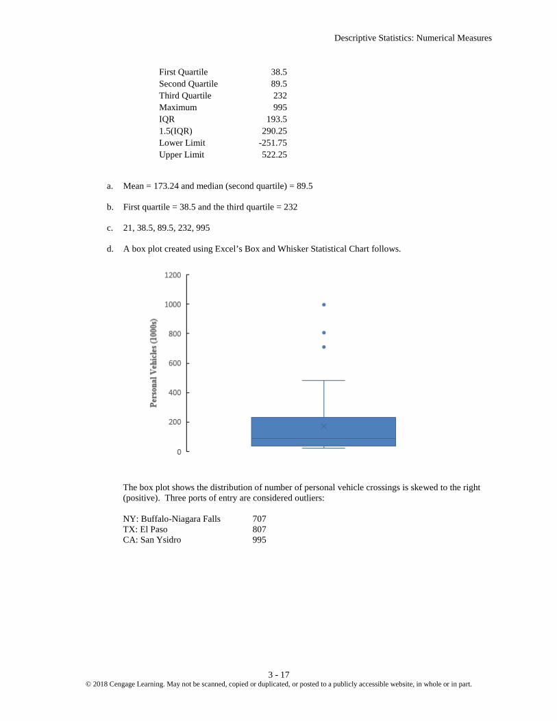
First Quartile 38.5 Second Quartile 89.5 Third Quartile 232 Maximum 995 IQR 193.5 1.5(IQR) 290.25 Lower Limit -251.75 Upper Limit 522.25
a. Mean = 173.24 and median (second quartile) = 89.5
b. First quartile = 38.5 and the third quartile = 232 c. 21, 38.5, 89.5, 232, 995 d. A box plot created using Excel’s Box and Whisker Statistical Chart follows.
The box plot shows the distribution of number of personal vehicle crossings is skewed to the right (positive). Three ports of entry are considered outliers: NY: Buffalo-Niagara Falls 707 TX: El Paso 807 CA: San Ysidro 995

Chapter 3
3 - 18 © 2018 Cengage Learning.May not be scanned, copied or duplicated, or posted to a publicly accessible website, in whole or in part.
55. a.
b. Negative relationship
c/d. Σ Σx x y yi i= = = = = =40 405
8 230 2305
46
Σ Σ Σ( )( ) ( ) ( )x x y y x x y yi i i i− − = − − = − =240 118 5202 2
2
2
( )( ) 240 601 5 1
( ) 118 5.43141 5 1
( ) 520 11.40181 5 1
60 .969(5.4314)(11.4018)
i ixy
ix
iy
xyxy
x y
x x y ys
n
x xs
n
y ys
n
sr
s s
Σ − − −= = = −
− −
Σ −= = =
− −
Σ −= = =
− −
−= = = −
Sample covariance = -60 The negative value of the sample covariance indicates a negative linear relationship Sample correlation coefficient = -.969 There is a strong negative linear relationship.
0
10
20
30
40
50
60
70
0 5 10 15 20
y
x

Descriptive Statistics: Numerical Measures
3 - 19 © 2018 Cengage Learning. May not be scanned, copied or duplicated, or posted to a publicly accessible website, in whole or in part.
56. a.
b. Positive relationship
c/d. Σ Σx x y yi i= = = = = =80 805
16 50 505
10
Σ Σ Σ( )( ) ( ) ( )x x y y x x y yi i i i− − = − = − =106 272 862 2
( )( ) 106 26.51 5 1
i ixy
x x y ysn
Σ − −= = =
− −
Sample covariance = 26.5 The positive value of the sample covariance indicates a positive linear relationship.
2( ) 272 8.2462
1 5 1i
xx xsn
Σ −= = =
− −
2( ) 86 4.6368
1 5 1i
yy ysn
Σ −= = =
− −
26.5 .693
(8.2462)(4.6368)xy
xyx y
sr
s s= = =
Sample correlation coefficient = .693 which indicates a moderately strongpositive linear relationship
02468
1012141618
0 5 10 15 20 25 30
y
x
Chapter 3
3 - 20 © 2018 Cengage Learning.May not be scanned, copied or duplicated, or posted to a publicly accessible website, in whole or in part.
58. Let x = miles per hour and y = miles per gallon
420 270420 42 270 2710 10i ix x y yΣ = = = Σ = = =
2 2( )( ) 475 ( ) 1660 ( ) 164i i i ix x y y x x y yΣ − − = − Σ − = Σ − =
2
2
( )( ) 475 52.77781 10 1
( ) 1660 13.58101 10 1
( ) 164 4.26871 10 1
52.7778 .91(13.5810)(4.2687)
i ixy
ix
iy
xyxy
x y
x x y ysn
x xsn
y ysn
sr
s s
Σ − − −= = = −
− −
Σ −= = =
− −
Σ −= = =
− −
−= = = −
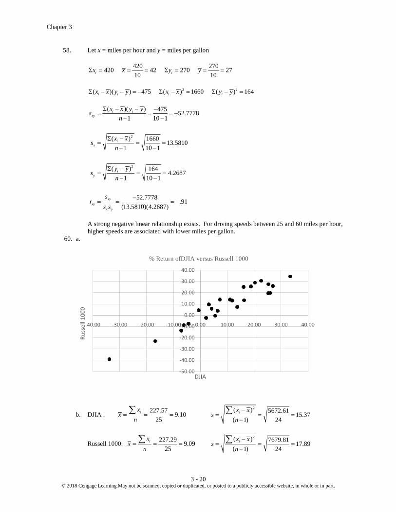
A strong negative linear relationship exists. For driving speeds between 25 and 60 miles per hour, higher speeds are associated with lower miles per gallon. 60. a.
b. DJIA : 227.57 9.1025
ixx
n= = =∑
2( ) 5672.61 15.37( 1) 24
ix xs
n−
= = =−
∑
Russell 1000: 227.29 9.0925
ixx
n= = =∑
2( ) 7679.81 17.89( 1) 24
ix xs
n−
= = =−
∑
-50.00
-40.00
-30.00
-20.00
-10.00
0.00
10.00
20.00
30.00
40.00
-40.00 -30.00 -20.00 -10.00 0.00 10.00 20.00 30.00 40.00
Russ
ell 1
000
DJIA
% Return ofDJIA versus Russell 1000

Descriptive Statistics: Numerical Measures
3 - 21 © 2018 Cengage Learning. May not be scanned, copied or duplicated, or posted to a publicly accessible website, in whole or in part.
c. 263.611 .959
(15.37)(17.89)xy
xyx y
sr
s s= = =
d. Based on this sample, the two indexes are very similar. They have a strong positive correlation. The variance of the Russell 1000 is slightly larger than that of the DJIA.
62. The data in ascending order follow.
Position Value
Position Value 1 0
11 3
2 0
12 3 3 1
13 3
4 1
14 4 5 1
15 4
6 1
16 5 7 1
17 5
8 2
18 6 9 3
19 6
10 3
20 7 a. The mean is 2.95 and the median is 3.
b. 2525( 1) (20 1) 5.25
100 100pL n= + = + =
First quartile or 25th percentile = 1 + . 25(1 – 1) = 1
7575( 1) (20 1) 15.75
100 100pL n= + = + =
Third quartile or 75th percentile = 4 + . 75(5 – 4) = 4.75
c. The range is 7 and the interquartile range is 4.75 – 1 = 3.75.
d. The variance is 4.37 and standard deviation is 2.09. e. Because most people dine out a relatively few times per week and a few families dine out very
frequently, we would expect the data to be positively skewed. The skewness measure of 0.34 indicates the data are somewhat skewed to the right.
f. The lower limit is –4.625 and the upper limit is 10.375. No values in the data are less than the lower
limit or greater than the upper limit, so there are no outliers. 64. a. The mean and median patient wait times for offices with a wait tracking system are 17.2 and 13.5,
respectively. The mean and median patient wait times for offices without a wait tracking system are 29.1 and 23.5, respectively.
b. The variance and standard deviation of patient wait times for offices with a wait tracking system are
86.2 and 9.3, respectively. The variance and standard deviation of patient wait times for offices without a wait tracking system are 275.7 and 16.6, respectively.
c. Offices with a wait tracking system have substantially shorter patient wait times than offices without
a wait tracking system.

Chapter 3
3 - 22 © 2018 Cengage Learning.May not be scanned, copied or duplicated, or posted to a publicly accessible website, in whole or in part.
d. 37 29.1 0.4816.6
z −= =
e. 37 17.2 2.139.3
z −= =
As indicated by the positive z–scores, both patients had wait times that exceeded the means of their
respective samples. Even though the patients had the same wait time, the z–score for the sixth patient in the sample who visited an office with a wait tracking system is much larger because that patient is part of a sample with a smaller mean and a smaller standard deviation.
f. The z–scores for all patients follow.
Without Wait Tracking System
With Wait Tracking System
-0.31 1.49 2.28 -0.67
-0.73 -0.34 -0.55 0.09 0.11 -0.56 0.90 2.13
-1.03 -0.88 -0.37 -0.45 -0.79 -0.56 0.48 -0.24
The z–scores do not indicate the existence of any outliers in either sample.
66. a. 20665 413.350
ixx
n= = =∑ This is slightly higher than the mean for the study.
b. 2( ) 69424.5 37.64
( 1) 49ix x
sn−
= = =−
∑
c. 2525( 1) (51) 12.75
100 100pL n= + = = First Quartile or Q1 = 374 + .75(384-374) = 381.5
7575( 1) (51) 38.25
100 100pL n= + = = Third Quartile or Q3 = 445 + .25(445-445) = 445
IQR = 445 – 381.5 = 63.5 LL = Q1 – 1.5 IQR = 381.5 – 1.5(63.5) = 286.25 UL = Q3+ 1.5 IQR = 445+ 1.5(63.5) = 540.25 There are no outliers.

Descriptive Statistics: Numerical Measures
3 - 23 © 2018 Cengage Learning. May not be scanned, copied or duplicated, or posted to a publicly accessible website, in whole or in part.
68. Excel’s MIN, QUARTILE.EXC, and MAX functions provided the following results; values for the IQR and the upper and lower limits are also shown.
Annual Household Income
Minimum 46.5 First Quartile 50.75 Second Quartile 52.1 Third Quartile 52.6 Maximum 64.5 IQR 1.85 1.5(IQR) 2.775 Lower Limit 47.975 Upper Limit 55.375
a. The data in ascending order follow:
46.5 48.7 49.4 51.2 51.3 51.6 52.1 52.1 52.2 52.4 52.5 52.9 53.4 64.5
5050( 1) (14 1) 7.5
100 100pL n= + = + =
Median or 50th percentile = 52.1 + . 5(52.1 –52.1) = 52.1
b. Percentage change = 52.1 55.5 100 6.1%55.5− = −
c. 2525( 1) (14 1) 3.75
100 100pL n= + = + =
25th percentile = 49.4 + .75(51.2 –49.4) = 50.75
7575( 1) (14 1) 11.25
100 100pL n= + = + =
75th percentile = 52.5 + .25(52.9 – 52.5) = 52.6
d. 46.5 50.75 52.1 52.6 64.5
e. 730.8 52.214
ixxnΣ
= = =
2
2 ( ) 208.12 16.00921 13
ix xsn
Σ −= = =
−
16.0092 4.0012s = =
The z-scores = ix xs− are shown below:

Chapter 3
3 - 24 © 2018 Cengage Learning.May not be scanned, copied or duplicated, or posted to a publicly accessible website, in whole or in part.
-1.42 -0.87 -0.70 -0.25 -0.22 -0.15 -0.02 -0.02 0.00 0.05 0.07 0.17 0.30 3.07
The last household income (64.5) has a z-score > 3 and is an outlier. Lower Limit = 1 1.5(IQR) 50.75 1.5(52.6 50.75) 47.98Q − = − − = Upper Limit = 3 1.5(IQR) 52.6 1.5(52.6 50.75) 55.38Q + = + − = Using this approach the first observation (46.5) and the last observation (64.5) would be consider outliers. The two approaches will not always provide the same results.
70. a. 4368 36412
ixx
nΣ
= = = rooms
b. 5484 $45712
iyy
nΣ
= = =
c.
It is difficult to see much of a relationship. When the number of rooms becomes larger, there is no indication that the cost per night increases. The cost per night may even decrease slightly.
ix iy ( )ix x− ( )iy y− 2( )ix x− 2( )iy y− ( )( )i ix x y y− −
220 499 -144 42 20.736 1,764 -6,048 727 340 363 -117 131,769 13,689 -42,471 285 585 -79 128 6,241 16,384 -10,112 273 495 -91 38 8,281 1,444 -3,458 145 495 -219 38 47,961 1,444 -8,322 213 279 -151 -178 22,801 31,684 26,878 398 279 34 -178 1,156 31,684 -6,052 343 455 -21 -2 441 4 42 250 595 -114 138 12,996 19,044 -15,732 414 367 50 -90 2,500 8,100 -4,500

Descriptive Statistics: Numerical Measures
3 - 25 © 2018 Cengage Learning. May not be scanned, copied or duplicated, or posted to a publicly accessible website, in whole or in part.
d.
2
2
( )( ) 74,359 6759.911 11
( ) 369,074 183.171 11
( ) 174,134 125.821 11
6759.91 .293(183.17)(125.82)
i ixy
ix
iy
xyxy
x y
x x y ys
n
x xs
n
y ys
n
sr
s s
Σ − − −= = = −
−
Σ −= = =
−
Σ −= = =
−
−= = = −
There is evidence of a slightly negative linear association between the number of rooms and the cost
per night for a double room. Although this is not a strong relationship, it suggests that the higher room rates tend to be associated with the smaller hotels.
This tends to make sense when you think about the economies of scale for the larger hotels. Many
of the amenities in terms of pools, equipment, spas, restaurants, and so on exist for all hotels in the Travel + Leisure top 50 hotels in the world. The smaller hotels tend to charge more for the rooms. The larger hotels can spread their fixed costs over many room and may actually be able to charge less per night and still achieve and nice profit. The larger hotels may also charge slightly less in an effort to obtain a higher occupancy rate. In any case, it appears that there is a slightly negative linear association between the number of rooms and the cost per night for a double room at the top hotels.
72. a.
ix iy ( )ix x− ( )iy y− 2( )ix x−
2( )iy y− ( )( )i ix x y y− − .407 .422 -.1458 -.0881 .0213 .0078 .0128 .429 .586 -.1238 .0759 .0153 .0058 -.0094 .417 .546 -.1358 .0359 .0184 .0013 -.0049 .569 .500 .0162 -.0101 .0003 .0001 -.0002 .569 .457 .0162 -.0531 .0003 .0028 -.0009 .533 .463 -.0198 -.0471 .0004 .0022 .0009 .724 .617 .1712 .1069 .0293 .0114 .0183 .500 .540 -.0528 .0299 .0028 .0009 -.0016 .577 .549 .0242 .0389 .0006 .0015 .0009
400 675 36 218 1,296 47,524 7,848 700 420 336 -37 112,896 1,369 -12,432
Total 369,074 174,134 -74,359

Chapter 3
3 - 26 © 2018 Cengage Learning.May not be scanned, copied or duplicated, or posted to a publicly accessible website, in whole or in part.
.692 .466 .1392 -.0441 .0194 .0019 -.0061
.500 .377 -.0528 -.1331 .0028 .0177 .0070
.731 .599 .1782 .0889 .0318 .0079 .0158
.643 .488 .0902 -.0221 .0081 .0005 -.0020
.448 .531 -.1048 .0209 .0110 .0004 -.0022 Total .1617 .0623 .0287
( )( ) .0287 .00221 14 1
i ixy
x x y ys
nΣ − −
= = =− −
2( ) .1617 .1115
1 14 1i
xx x
sn
Σ −= = =
− −
2( ) .0623 .0692
1 14 1i
yy y
sn
Σ −= = =
− −
.0022 .286
.1115(.0692)xy
xyx y
sr
s s= = = +
b. There is a low positive correlation between a major league baseball team’s winning percentage
during spring training and its winning percentage during the regular season. The spring training record should not be expected to be a good indicator of how a team will play during the regular season.
Spring training consists of practice games between teams with the outcome as to who wins or who
loses not counting in the regular season standings or affecting the chances of making the playoffs. Teams use spring training to help players regain their timing and evaluate new players. Substitutions are frequent with the regular or better players rarely playing an entire spring training game. Winning is not the primary goal in spring training games. A low correlation between spring training winning percentage and regular season winning percentage should be anticipated.
74.
wi xi wi xi ix x− 2( )ix x− 2( )i iw x x− 2( )ix x− 2( )i iw x x− 10 47 470 -13.68 187.1424 1871.42 187.26 1872.58
40 52 2080 -8.68 75.3424 3013.70 75.42 3016.62 150 57 8550 -3.68 13..5424 2031.36 13.57 2036.01 175 62 10850 +1.32 1.7424 304.92 1.73 302.98 75 67 5025 +6.32 39.9424 2995.68 39.89 2991.69 15 72 1080 +11.32 128.1424 1922.14 128.05 1920.71 10 77 770 +16.32 266.3424 2663.42 266.20 2662.05
475 28,825 14,802.64 14802.63 Columns 5 and 6 are calculated with rounding, while columns 7 and 8 are based on unrounded calculations.
a. 28,825 60.68475
x = =
b. 2 14,802.64 31.23474
s = =
31.23 5.59s = =

Descriptive Statistics: Numerical Measures
3 - 27 © 2018 Cengage Learning. May not be scanned, copied or duplicated, or posted to a publicly accessible website, in whole or in part.
Introduction to Probability
4 - 1 © 2018 Cengage Learning. May not be scanned, copied or duplicated, or posted to a publicly accessible website, in whole or in part.
Chapter 4 Introduction to Probability Solutions:
2. 6 6! 6 5 4 3 2 1 203 3!3! (3 2 1)(3 2 1)
⋅ ⋅ ⋅ ⋅ ⋅= = = ⋅ ⋅ ⋅ ⋅
ABC ACE BCD BEF ABD ACF BCE CDE ABE ADE BCF CDF ABF ADF BDE CEF ACD AEF BDF DEF
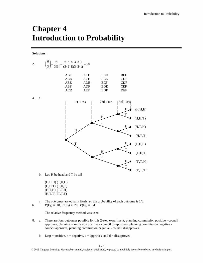
4. a.
b. Let: H be head and T be tail (H,H,H) (T,H,H) (H,H,T) (T,H,T) (H,T,H) (T,T,H) (H,T,T) (T,T,T) c. The outcomes are equally likely, so the probability of each outcome is 1/8. 6. P(E1) = .40, P(E2) = .26, P(E3) = .34 The relative frequency method was used. 8. a. There are four outcomes possible for this 2-step experiment; planning commission positive - council
approves; planning commission positive - council disapproves; planning commission negative - council approves; planning commission negative - council disapproves.
b. Letp = positive, n = negative, a = approves, and d = disapproves
H
T
H
T
H
T
HT
H
T
H
T
HT
(H,H,H)
(H,H,T)
(H,T,H)
(H,T,T)
(T,H,H)
(T,H,T)
(T,T,H)
(T,T,T)
1st Toss 2nd Toss 3rd Toss

Chapter 4
4 - 2 © 2018 Cengage Learning. May not be scanned, copied or duplicated, or posted to a publicly accessible website, in whole or in part.
9. 50 50! 50 49 48 47 230,3004 4!46! 4 3 2 1
⋅ ⋅ ⋅= = = ⋅ ⋅ ⋅
10. a. Using the table provided, 86.5% of Delta flights arrive on time. P(on-time arrival) = .865 b. Three of the 10 airlines have less than two mishandled baggage reports per 1000 passengers. P(Less than 2) = 3/10 = .30 c. Five of the 10 airlines have more than one customer complaints per 1000 passengers. P(more than 1) = 5/10 = .50 d. P(not on time) = 1 - P(on time) = 1 - .871 = .129
12. a. Step 1: Use the counting rule for combinations:
Step 2: There are 35 ways to select the red Powerball from digits 1 to 35 Total number of Powerball lottery outcomes: (5,006,386) x (35) = 175,223,510 b. Probability of winning the lottery: 1 chance in 175,223,510
.
Planning Commission Council
p
n
a
d
a
d
(p, a)
(p, d)
(n, a)
(n, d)

Introduction to Probability
4 - 3 © 2018 Cengage Learning. May not be scanned, copied or duplicated, or posted to a publicly accessible website, in whole or in part.
= 1/(175,223,510) = .000000005707 14. a. P(E2) = 1/4 b. P(any 2 outcomes) = 1/4 + 1/4 = 1/2 c. P(any 3 outcomes) = 1/4 + 1/4 + 1/4 = 3/4 15. a. S = {ace of clubs, ace of diamonds, ace of hearts, ace of spades} b. S = {2 of clubs, 3 of clubs, . . . , 10 of clubs, J of clubs, Q of clubs, K of clubs, A of clubs} c. There are 12; jack, queen, or king in each of the four suits. d. For a: 4/52 = 1/13 = .08 For b: 13/52 = 1/4 = .25 For c: 12/52 = .23 16. a. (6)(6) = 36 sample points b.
c. 6/36 = 1/6 d. 10/36 = 5/18 e. No. P(odd) = 18/36 = P(even) = 18/36 or 1/2 for both. f. Classical. A probability of 1/36 is assigned to each experimental outcome.
.
1
2
3
4
5
6
1 2 3 4 5 6
2
3
4
5
6
7
3
4
5
6
7
8
4
5
6
7
8
9
5
6
7
8
9
10 11
10
9
8
7
6 7
8
9
10
11
12
Die 1
Total for Both
Die 2

Chapter 4
4 - 4 © 2018 Cengage Learning. May not be scanned, copied or duplicated, or posted to a publicly accessible website, in whole or in part.
17. a. (4,6), (4,7), (4,8) b. .05 + .10 + .15 = .30 c. (2,8), (3,8), (4,8) d. .05 + .05 + .15 = .25 e. Both are over budget only with (4,8) and therefore probability = .15 18. a. Let C = corporate headquarters located in California = 53/500 = .106 b. Let N = corporate headquarters located in New York T = corporate headquarters located in Texas P(N) = 50/500 = .100 P(T) = 52/500 = .104 Located in California, New York, or Texas
c. Let A = corporate headquarters located in one of the eight states Total number of companies with corporate headquarters in the eight states = 283 P(A) = 283/500 = .566
Over half the Fortune 500 companies have corporate headquartered located in these eight states. 20. a.
Age
Experimental Financially Number of Outcome Independent Responses Probability
E1 16 to 20 191 191/944 = 0.2023 E2 21 to 24 467 467/944 = 0.4947 E3 25 to 27 244 244/944 = 0.2585 E4 28 or older 42 42/944 = 0.0445
944
b. c. d. The probability of being financially independent before the age of 25, .6970, seems high given the
general economic conditions. It appears that the teenagers who responded to this survey may have unrealistic expectations about becoming financially independent at a relatively young age.
Introduction to Probability
4 - 5 © 2018 Cengage Learning. May not be scanned, copied or duplicated, or posted to a publicly accessible website, in whole or in part.
22. E1=E2=E3=E4=E5= 0.2 for each A= E1, E2 B= E3, E4 C= E2, E3, E5 a. P(A) = .2+.2=.40, P(B) = .2+.2=.40, P(C) = .2+.2+.2=.60 b. P(A ∪ B) = P(E1, E2, E3, E4) = .80. Yes P(A ∪ B) = P(A) + P(B) because they do not have any outcomes in common.. c. Ac = {E3, E4, E5} Cc = {E1, E4} P(Ac) = .60 P(Cc) = .40 d. A ∪ Bc = {E1, E2, E5} P(A ∪ Bc) = .60 e. P(B ∪ C) = P(E2, E3, E4, E5) = .80 23. a. P(A) = P(E1) + P(E4) + P(E6) = .05 + .25 + .10 = .40 P(B) = P(E2) + P(E4) + P(E7) = .20 + .25 + .05 = .50 P(C) = P(E2) + P(E3) + P(E5) + P(E7) = .20 + .20 + .15 + .05 = .60 b. A ∪ B = {E1, E2, E4, E6, E7} P(A ∪ B) = P(E1) + P(E2) + P(E4) + P(E6) + P(E7) OR P(A ∪ B) = P(A) + P(B) – P(A ∩ B) c. A ∩ B = {E4} P(A ∩ B) = P(E4) = .25 d. Yes, they are mutually exclusive because they do not have any outcomes in common (there is no intersection between them). e. Bc = {E1, E3, E5, E6}; P(Bc) = P(E1) + P(E3) + P(E5) + P(E6) = .05 + .20 + .15 + .10 = .50 24. Let E = experience exceeded expectations M = experience met expectations S = experience fell short of expectations N = no response a. Percentage of respondents that said their experience exceeded expectations = 1 – all other responses = 1 – { P(N)+ P(S) + P(M) } = 1- (.04+.26+.65) = .05 P(E) = .05 b. P(M ∪ E) = P(M) + P(E) = .65 + .05 = .70 26. a. Let D = Domestic Equity Fund P(D) = 16/25 = .64 b. Let A = 4- or 5-star rating 13 funds were rated 3-star of less; thus, 25 – 13 = 12 funds must be 4-star or 5-star. P(A) = 12/25 = .48
Chapter 4
4 - 6 © 2018 Cengage Learning. May not be scanned, copied or duplicated, or posted to a publicly accessible website, in whole or in part.
c. 7 Domestic Equity funds were rated 4-star and 2 were rated 5-star. Thus, 9 funds were Domestic
Equity funds and were rated 4-star or 5-star P(D∩A) = 9/25 = .36 d. P(D∪A) = P(D) + P(A) - P(D∩A) = .64 + .48 - .36 = .76 28. Let: B = rented a car for business reasons P = rented a car for personal reasons a. P(B ∪ P) = P(B) + P(P) - P(B ∩ P) = .54 + .458 - .30 = .698 b. P(Neither) = 1 - .698 = .302
30. a. (A B) .40(A B) .6667(B) .60
PPP
∩= = =
b. (A B) .40(B A) .80(A) .50
PPP
∩= = =
c. No because P(A | B) ≠P(A) 32. a. Dividing each entry in the table by 500 yields the following (rounding to two digits):
Yes No Totals Men 0.210 0.282 0.492 Women 0.186 0.322 0.508
Totals 0.396 0.604 1.00
Let M = 18-34-year-old man, W = 18-34-year-old woman, Y = responded yes, N = responded no
b. P(M) = .492, P(W) = .508 P(Y) = .396, P(N) = .604
c. P(Y|M) = .210/.492 = .4268 d. P(Y|W) = .186/.508 = .3661 e. P(Y) = .396/1 = .396 f. P(M) = .492 in the sample. Yes, this seems like a good representative sample based on gender.
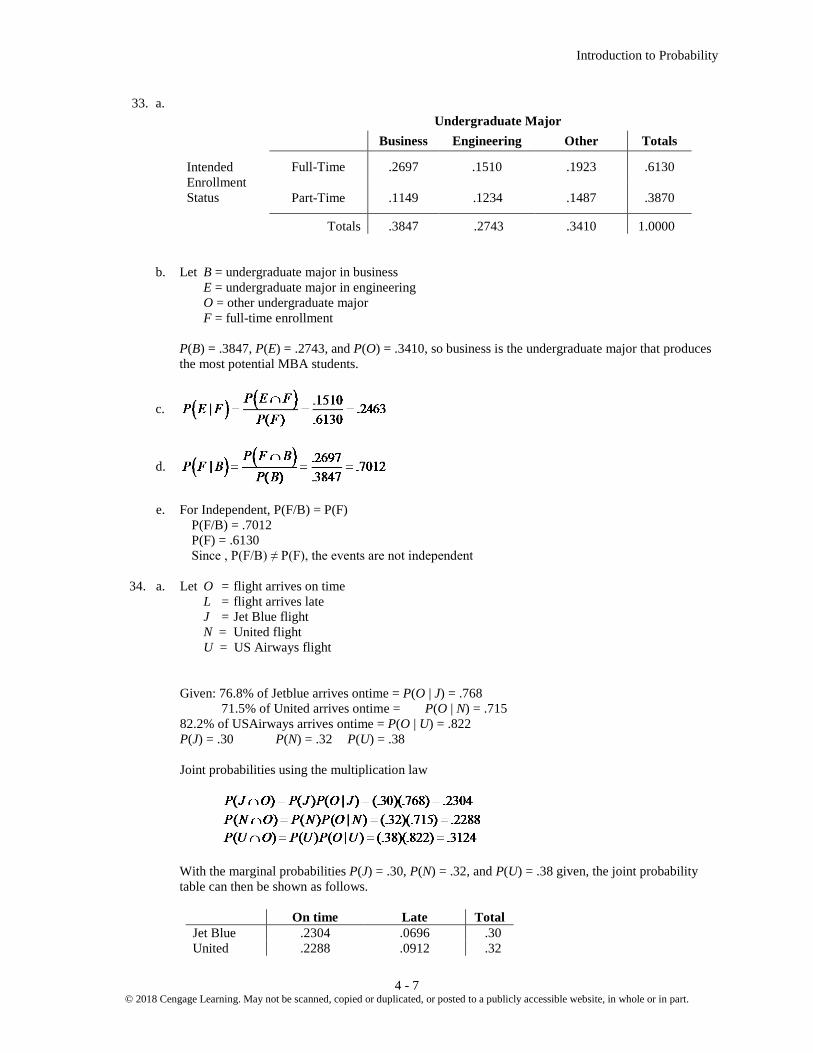
Introduction to Probability
4 - 7 © 2018 Cengage Learning. May not be scanned, copied or duplicated, or posted to a publicly accessible website, in whole or in part.
33. a.
Undergraduate Major Business Engineering Other Totals
Intended Enrollment Status
Full-Time .2697 .1510 .1923 .6130
Part-Time .1149 .1234 .1487 .3870
Totals .3847 .2743 .3410 1.0000
b. Let B = undergraduate major in business E = undergraduate major in engineering O = other undergraduate major F = full-time enrollment P(B) = .3847, P(E) = .2743, and P(O) = .3410, so business is the undergraduate major that produces
the most potential MBA students.
c.
d.
e. For Independent, P(F/B) = P(F)
P(F/B) = .7012 P(F) = .6130 Since , P(F/B) ≠ P(F), the events are not independent
34. a. Let O = flight arrives on time L = flight arrives late J = Jet Blue flight N = United flight U = US Airways flight Given: 76.8% of Jetblue arrives ontime = P(O | J) = .768 71.5% of United arrives ontime = P(O | N) = .715 82.2% of USAirways arrives ontime = P(O | U) = .822
P(J) = .30 P(N) = .32 P(U) = .38 Joint probabilities using the multiplication law With the marginal probabilities P(J) = .30, P(N) = .32, and P(U) = .38 given, the joint probability
table can then be shown as follows.
On time Late Total Jet Blue .2304 .0696 .30 United .2288 .0912 .32
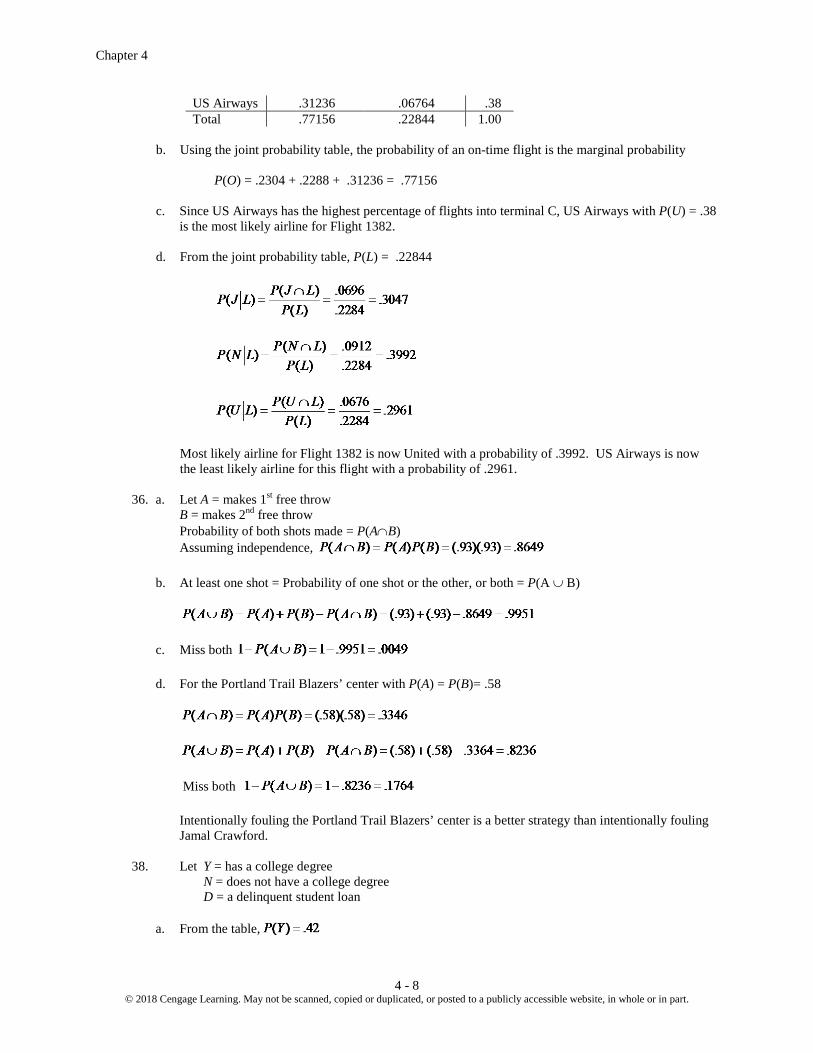
Chapter 4
4 - 8 © 2018 Cengage Learning. May not be scanned, copied or duplicated, or posted to a publicly accessible website, in whole or in part.
US Airways .31236 .06764 .38 Total .77156 .22844 1.00
b. Using the joint probability table, the probability of an on-time flight is the marginal probability P(O) = .2304 + .2288 + .31236 = .77156 c. Since US Airways has the highest percentage of flights into terminal C, US Airways with P(U) = .38
is the most likely airline for Flight 1382. d. From the joint probability table, P(L) = .22844
Most likely airline for Flight 1382 is now United with a probability of .3992. US Airways is now the least likely airline for this flight with a probability of .2961.
36. a. Let A = makes 1st free throw B = makes 2nd free throw Probability of both shots made = P(A∩B) Assuming independence, b. At least one shot = Probability of one shot or the other, or both = P(A ∪ B) c. Miss both d. For the Portland Trail Blazers’ center with P(A) = P(B)= .58 Miss both Intentionally fouling the Portland Trail Blazers’ center is a better strategy than intentionally fouling
Jamal Crawford. 38. Let Y = has a college degree N = does not have a college degree D = a delinquent student loan a. From the table,

Introduction to Probability
4 - 9 © 2018 Cengage Learning. May not be scanned, copied or duplicated, or posted to a publicly accessible website, in whole or in part.
b. From the table,
c.
d.
e. Individuals who obtained a college degree have a .3810 probability of a delinquent student loan
while individuals who dropped out without obtaining a college degree have a .5862 probability of a delinquent student loan. Not obtaining a college degree will lead to a greater probability of struggling to payback the student loan and will likely lead to financial problems in the future.
39. a. Yes, since P(A1∩ A2) = 0 b. P(A1∩ B) = P(A1)P(B | A1) = .40(.20) = .08 P(A2∩ B) = P(A2)P(B | A2) = .60(.05) = .03 c. P(B) = P(A1∩ B) + P(A2∩ B) = .08 + .03 = .11
d. 1.08(A B) .7273.11
P = =
2.03(A B) .2727.11
P = =
40. a. P(B ∩ A1) = P(A1)P(B | A1) = (.20)(.50) = .10 P(B ∩ A2) = P(A2)P(B | A2) = (.50)(.40) = .20 P(B ∩ A3) = P(A3)P(B | A3) = (.30)(.30) = .09
b. 2.20(A B) .51
.10 .20 .09P = =
+ +
c.
Events P(Ai) P(B | Ai) P(Ai∩ B) P(Ai | B) A1 .20 .50 .10 .26 A2 .50 .40 .20 .51 A3 .30 .30 .09 .23
1.00 .39 1.00 42. M = missed payment D1 = customer defaults D2 = customer does not default P(D1) = .05 P(D2) = .95 P(M | D2) = .2 P(M | D1) = 1
a. 1 11
1 1 2 2
(D ) (M D ) (.05)(1) .05(D M) .21(D ) (M D ) (D ) (M D ) (.05)(1) (.95)(.2) .24
P PP
P P P P= = = =
+ +

Chapter 4
4 - 10 © 2018 Cengage Learning. May not be scanned, copied or duplicated, or posted to a publicly accessible website, in whole or in part.
Alternative Solutions for Part a: Bayes Table
Events P(Di) P(M | Di) P(Di∩ M) P(Di | M) D1 .05 1.0 .05 .21 D2 .95 .20 .19 .79
1.00 .24 1.00 From the Bayes Table, P(D1/M) = .21 Probability Table
M Mc Totals
D1 1*.05 =
.05 .05-.05 =
0 .05
D2
.2*.95 =
.19 .95- .19 =
.76 .95
Totals 0.24 0.76 1.00 From the Probability Table, P(S1/B) = .05/.24 = .21 b. Yes, the probability of default is greater than .20. 44. M = the current visitor to the ParFore website is a male F = the current visitor to the Parfore website is a female D = a visitor to the ParFore website previously visited the Dillard website a. Using past history, P(F) = .40. b. P(M) = .60, , and
The revised probability that the current visitor is a female is .6667. ParFore should display the special offer that appeals to female visitors. Alternative Solutions for Part b: Bayes Table
Events P(genderi) P(D | genderi) P(genderi∩ D) P(genderi | D) F .4 .3 .12 .6667 M .6 .1 .06 .3333 1.00 .18 1.00
From the Bayes Table, P(F/D) = .6667 Probability Table
D Dc Totals
F .3*.4=
.12 .4-.12 =
.28 .4 M .6- .06 = .6

Introduction to Probability
4 - 11 © 2018 Cengage Learning. May not be scanned, copied or duplicated, or posted to a publicly accessible website, in whole or in part.
.1*.6 = .06
.54
Totals 0.18 0.82 1.00 From the Probability Table, P(F/D) = .12/.18 = .6667 46. a. 422 + 181 + 80 + 121 + 201 = 1005 respondents b. Most frequent response a day or less; Probability = 422/1005 = .4199 c. 201/1005 = .20 d. Responses of 2 days, 3 days, and 4 or more days = 181 + 80 + 121 = 382 Probability = 382/1005 = .3801 48. a. There are a total of 1364 responses. Dividing each entry by 1364 provides the following joint
probability table.
A B Total Female .2896 .2133 .5029 Male .2368 .2603 .4971 Total .5264 .4736 1.0000
b. The marginal probability of a female is .5029 from above. c. Let A = uses social media and other websites to voice opinions about television programs F = female respondent
OR From raw data, 395/686 = .5758
d. For Independent, P(A/F) = P(A) P(A/F) = .5758 P(A) = .5264 Since , P(A/F) ≠ P(A), the events are not independent
50. a. Probability of the event = P(average) + P(above average) + P(excellent)
= 1150
1450
1350
+ + = .22 + .28 + .26 = .76
b. Probability of the event = P(poor) + P(below average)
= 450
850
24+ =.
52. a.
More Than One Age Group Yes No Total 23 and Under .1026 .0996 .2022 24 – 26 .1482 .1878 .3360 27 – 30 .0917 .1328 .2245 31 – 25 .0327 .0956 .1283

Chapter 4
4 - 12 © 2018 Cengage Learning. May not be scanned, copied or duplicated, or posted to a publicly accessible website, in whole or in part.
36 and Over .0253 .0837 .1090 Total .4004 .5996 1.0000
Although the columns appear to add up to .4005 and .5995, the actual calculation resulting from using raw column totals results in 808/2018 =.4004 and 1210/2018 = .5996. Students may have either answer, and both could be considered correct.
b. Marginal probability .2022 c. .2245 + .1283 + .1090 = .4618 d. Marginal probability = 808/2018 = .4004 See note above. 54. a. P(Not Okay) = .1485 + .2273 + .4008 = .7766
b.
c.
d. The attitude about this practice is not independent of the age of the respondent. One way to show
this follows. P(Okay) = 1 – P(Not Okay) = 1 - .7766 = .2234
Since , attitude is not independent of the age of the respondent.
e.
There is a higher probability the 50+ year olds will not be okay with this practice. 56. a. P(A) = 200/800 = .25 b. P(B) = 100/800 = .125 c. P(A ∩ B) = 10/800 = .0125
d. P(A | B) = P(A ∩ B)/P(B) = .0125/.125 = .10 OR From raw data, 10 / 100 = .10 e. No, P(A | B) ≠P(A) or .10 ≠.25

Introduction to Probability
4 - 13 © 2018 Cengage Learning. May not be scanned, copied or duplicated, or posted to a publicly accessible website, in whole or in part.
58. a. Let = student studied abroad
= student did not study abroad F = female student M = male student P(A1) = .095 P(A2) = = 1 .095 = .905 P(F | A1) = .60 P(F | A2) = .49 Tabular computations
Events P(Ai) P(F|Ai) P(Ai∩F) P(Ai|F) A1 .095 .60 .0570 .1139 A2 .905 .49 .4435 .8861
P(F) = .5005
P(A1|F) = .1139 b.
Events P(Ai) P(M|Ai) P(Ai∩M) P(Ai|M)
A1 .095 .40 .0380 .0761
A2 .905 .51 .4615 .9239
P(M) = .4995
P(A1|M) = .0761 Alternative Solution for Part a and b: Probability Table
F M Totals
A1 .6*.095 =
.0570
.095-.0570 or .4*.095 =
= .0380 .095
A2
.49*.905 =
.4435
.905-.4435 or
.51*.905 = .4615 .905
Totals 0.5005 0.4995 1.00 From the Probability Table, P(A1/F) = .0570/.5005 = .1139 and P(A1/M) = .0380/.4995 = .0761 c. From above, P(F) = .5005 and P(M) = .4995, so almost 50/50 female and male full-time students.

Chapter 4
4 - 14 © 2018 Cengage Learning. May not be scanned, copied or duplicated, or posted to a publicly accessible website, in whole or in part.
60. a.
( ) ( ) ( )( ) ( ) ( ) ( )
( )( )( )( ) ( )( )
ham |hamham|
ham |ham spam |spam
.90 .0015 .2093
.90 .0015 .10 .051
P P shipping!P shipping!
P P shipping! P P shipping!=
+
= =+
If a message includes the word shipping!, the probability the message is spam is high (.7910), and so
the message should be flagged as spam. b.
A message that includes the word today! is more likely to be spam. This is because P(today!|spam) is larger than P(here!|spam). Because today! occurs more often in unwanted messages (spam), it is easier to distinguish spam from ham in messages that include today!.
c.
A message that includes the word fingertips! is more likely to be spam. d. It is easier to distinguish spam from ham when a word occurs more often in unwanted messages
(spam) and/or less often in legitimate messages (ham).

5 - 1 © 2018 Cengage Learning.May not be scanned, copied or duplicated, or posted to a publicly accessible website, in whole or in part.
Chapter 5 Discrete Probability Distributions Solutions: 1. a. Head, Head (H,H) Head, Tail (H,T) Tail, Head (T,H) Tail, Tail (T,T) b. x = number of heads on two coin tosses c.
Outcome Values of x (H,H) 2 (H,T) 1 (T,H) 1 (T,T) 0
d. Discrete. It may assume 3 values: 0, 1, and 2. 2. a. Let x = time (in minutes) to assemble the product. b. It may assume any positive value: x> 0. c. Continuous 3. Let Y = position is offered N = position is not offered a. S = {(Y,Y,Y), (Y,Y,N), (Y,N,Y), (N,Y,Y), (Y,N,N), (N,Y,N), (N,N,Y), (N,N,N)} b. Let N = number of offers made; N is a discrete random variable. c. Experimental Outcome (Y,Y,Y) (Y,Y,N) (Y,N,Y) (N,Y,Y) (Y,N,N) (N,Y,N) (N,N,Y) (N,N,N) Value of N 3 2 2 2 1 1 1 0 4. 0, 1, 2, 3, 4, 5, 6, 7, 8, 9 6. a. values: 0,1,2,...,20 discrete b. values: 0,1,2,... discrete c. values: 0,1,2,...,50 discrete d. values: 0 ≤x≤ 8 continuous e. values: x> 0

Chapter 5
5 - 2 © 2018 Cengage Learning.May not be scanned, copied or duplicated, or posted to a publicly accessible website, in whole or in part.
continuous 7. a. f (x) ≥ 0 for all values of x. Σf (x) = 1 Therefore, it is a proper probability distribution. b. Probability x = 30 is f (30) = .25 c. Probability x≤ 25 is f (20) + f (25) = .20 + .15 = .35 d. Probability x> 30 is f (35) = .40 8. a. Let x = number of operating rooms in use on any given day
x f (x) 1 3/20 = .15 2 5/20 = .25 3 8/20 = .40 4 4/20 = .20 Total 1.00
b.
c. f (x) ≥ 0 for x = 1,2,3,4. Σf (x) = 1 10. a.Senior Executives
x f(x) 1 0.05 2 0.09 3 0.03 4 0.42 5 0.41
1.00 b. Middle Managers
x f(x) 1 0.04

Discrete Probability Distributions
5 - 3 © 2018 Cengage Learning. May not be scanned, copied or duplicated, or posted to a publicly accessible website, in whole or in part.
2 0.10 3 0.12 4 0.46 5 0.28
1.00 c. P(4 or 5) = f (4) + f (5) = 0.42 + 0.41 = 0.83 d. Probability of very satisfied: 0.28 e. Senior executives appear to be more satisfied than middle managers. 83% of senior executives have
a score of 4 or 5 with 41% reporting a 5. Only 28% of middle managers report being very satisfied. 12. a. Yes; f (x) ≥ 0. Σf (x) = 1 b. f (500,000) + f (600,000) = .10 + .05 = .15 c. f (100,000) = .10 14. a. f (200) = 1 –f (–100) –f (0) –f (50) –f (100) –f (150) = 1 – .95 = .05 This is the probability MRA will have a $200,000 profit. b. P(Profit) = f (50) + f (100) + f (150) + f (200) = .30 + .25 + .10 + .05 = .70 c. P(at least 100) = f (100) + f (150) + f (200) = .25 + .10 +.05 = .40 16. a.
y f (y) y f (y) 2 .2 .4 4 .3 1.2 7 .4 2.8 8 .1 .8 1.0 5.2
E(y) = µ = 5.2 b.
y y - µ (y - µ)2 f (y) (y - µ)2f (y) 2 -3.20 10.24 .20 2.048 4 -1.20 1.44 .30 .432 7 1.80 3.24 .40 1.296 8 2.80 7.84 .10 .784 4.560
( ) 4.56
4.56 2.14
Var y
σ
=
= =

Chapter 5
5 - 4 © 2018 Cengage Learning.May not be scanned, copied or duplicated, or posted to a publicly accessible website, in whole or in part.
18. a/b/ Owner occupied
x f (x) xf (x) x - µ (x - µ)2 (x - µ)2f (x) 0 .2188 .0000 -1.1825 1.3982 .3060 1 .5484 .5484 -.1825 .0333 .0183 2 .1241 .2483 .8175 .6684 .0830 3 .0489 .1466 1.8175 3.3035 .1614 4 .0598 .2393 2.8175 7.9386 .4749
Total 1.0000 1.1825 1.0435 ↑ ↑ E(x) Var(x)
c/d. Renter occupied
y f (y) yf (y) y - µ (y - µ)2 (y - µ)2f (y) 0 .2497 .0000 -1.2180 1.4835 .3704 1 .4816 .4816 -.2180 .0475 .0229 2 .1401 .2801 .7820 .6115 .0856 3 .0583 .1749 1.7820 3.1755 .1851 4 .0703 .2814 2.7820 7.7395 .5444
Total 1.0000 1.2180 1.2085 ↑ ↑ E(y) Var(y)
e. The expected number of times that owner-occupied units have a water supply stoppage lasting 6 or more hours in the past 3 months is 1.1825, slightly less than the expected value of 1.2180 for renter-occupied units. And, the variability is somewhat less for owner-occupied units (1.0435) as compared to renter-occupied units (1.2085).
20. a.
The expected value of the insurance claim is $430. If the company charges $430 for this type of
collision coverage, it would break even. b. From the point of view of the policyholder, the expected gain is as follows:
Expected Gain = Expected claim payout – Cost of insurance coverage = $430 - $520 = -$90 The policyholder is concerned that an accident will result in a big repair bill if there is no insurance
coverage. So even though the policyholder has an expected annual loss of $90, the insurance isprotecting against a large loss.
x f(x) xf(x) 0 .85 0
500 .04 20 1000 .04 40 3000 .03 90 5000 .02 100 8000 .01 80 10000 .01 100
Total 1.00 430

Discrete Probability Distributions
5 - 5 © 2018 Cengage Learning. May not be scanned, copied or duplicated, or posted to a publicly accessible website, in whole or in part.
21. Excel Tables Computations for a, b, and c
a. E(x)= Σx f (x) = 0.05(1) + 0.09(2) + 0.03(3) + 0.42(4) + 0.41(5) = 4.05 b. E(x)= Σx f (x) = 0.04(1) + 0.10(2) + 0.12(3) + 0.46(4) + 0.28(5) = 3.84 c. Executives: σ 2 = Σ (x -µ)2 f(x) = 1.25 Middle Managers: σ 2 = Σ (x -µ)2 f(x) = 1.13 d. Executives: σ = 1.12 Middle Managers: σ = 1.07 e. The senior executives have a higher average score: 4.05 vs. 3.84 for the middle managers. The
executives also have a slightly higher standard deviation. 24. a. Medium E(x) = Σx f (x) = 50 (.20) + 150 (.50) + 200 (.30) = 145 Large: E(x) = Σx f (x) = 0 (.20) + 100 (.50) + 300 (.30) = 140 Medium preferred. b. Medium
x f (x) x - µ (x - µ)2 (x - µ)2f (x) 50 .20 -95 9025 1805.0 150 .50 5 25 12.5 200 .30 55 3025 907.5
σ 2 = 2725.0 Large
y f (y) y - µ (y - µ)2 (y - µ)2f (y) 0 .20 -140 19600 3920
100 .50 -40 1600 800

Chapter 5
5 - 6 © 2018 Cengage Learning.May not be scanned, copied or duplicated, or posted to a publicly accessible website, in whole or in part.
300 .30 160 25600 7680 σ 2 = 12,400 Medium preferred due to less variance. 25. a. ( ) .2(50) .5(30) .3(40) 37= + + =E x
( ) .2(80) .5(50) .3(60) 59= + + =E y
2 2 2( ) .2(50 37) .5(30 37) .3(40 37) 61Var x = − + − + − =
2 2 2( ) .2(80 59) .5(50 59) .3(60 59) 129Var y = − + − + − = b.
x + y f(x +y) 130 .2 80 .5
100 .3 c.
x + y f(x +y) (x + y)f(x + y) x + y – E(x + y) 2[ ( )]+ − +x y E x y 2[ ( )] ( )+ − + +x y E x y f x y 130 .2 26 34 1156 231.2 80 .5 40 -16 256 128.0
100 .3 30 4 16 4.8 E(x + y) = 96 Var(x + y) = 364
d. [ ( ) ( ) ( )] / 2 (364 61 129) / 2 87σ = + − − = − − =xy Var x y Var x Var y
Var(x) = 61 and Var(y) =129 were computed in part (a), so
61 7.8102σ = =x 129 11.3578yσ = =
87 .98(7.8102)(11.3578)
xyxy
x y
σρ
σ σ= = =
The random variables x and y are positively related. Both the covariance and correlation coefficient
are positive. Indeed, they are very highly correlated; thecorrelation coefficient is almost equal to 1. e. ( ) ( ) ( ) 2 61 129 2(87) 364xyVar x y Var x Var y σ+ = + + = + + =
Var(x) + Var(y) = 61 + 129 = 190 The variance of the sum of x and y is greater than the sum of the variances by twotimes the covariance: 2(87) = 174. The reason it is positive is that, in thiscase the variables are positively related. Whenever two random variables arepositively related, the variance of the sum of the randomly variables will be greater than the sum of the variances of the individual random variables.
Discrete Probability Distributions
5 - 7 © 2018 Cengage Learning. May not be scanned, copied or duplicated, or posted to a publicly accessible website, in whole or in part.
26. a. The standard deviation for these two stocks is the square root of the variance. ( ) 25 5%x Var xσ = = = ( ) 1 1%y Var yσ = = = Investments in Stock 1 would be considered riskier than investments in Stock 2 because the standard
deviation is higher. Note that if the return for Stock 1 falls 8.45/5 = 1.69 or more standard deviation below its expected value, an investor in that stock will experience a loss. The return for Stock 2 would have to fall 3.2 standard deviations below its expected value before an investor in that stock would experience a loss.
b. Since x represents the percent return for investing in Stock 1, the expected return forinvesting $100
in Stock 1 is $8.45 and the standard deviation is $5.00. So to get the expected return and standard deviation for a $500 investment we just multiplyby 5.
Expected return ($500 investment) = 5($8.45) = $42.25 Standard deviation ($500 investment) = 5($5.00) = $25.00 c. Since x represents the percent return for investing in Stock 1 and y represents thepercent return for
investing in Stock 2, we want to compute the expected valueand variance for .5x + .5y. E(.5x + .5y) = .5E(x) + .5E(y) = .5(8.45) + .5(3.2) = 4.225 + 1.6 = 5.825
2 2
2 2
(.5 .5 ) .5 ( ) .5 ( ) 2(.5)(.5)
(.5) (25) (.5) (1) 2(.5)(.5)( 3)
6.25 .25 1.50 5
xyVar x y Var x Var y σ+ = + +
= + + −
= + − =
.5 .5 5 2.236σ + = =x y d. Since x represents the percent return for investing in Stock 1 and y represents thepercent return for
investing in Stock 2, we want to compute the expected valueand variance for .7x + .3y. E(.7x + .3y) = .7E(x) + .3E(y) = .7(8.45) + .3(3.2)=5.915 + .96= 6.875
2 2
2 2
(.7 .3 ) .7 ( ) .3 ( ) 2(.7)(.3)
.7 (25) .3 (1) 2(.7)(.3)( 3)
12.25 .09 1.26 11.08
xyVar x y Var x Var y σ+ = + +
= + + −
= + − =
.7 .3 11.08 3.329x yσ + = = e. The standard deviations of x and y were computed in part (a). The correlationcoefficient is given by
3 .6(5)(1)
xyxy
x y
σρ
σ σ−
= = = −
There is a fairly strong negative relationship between the variables.

Chapter 5
5 - 8 © 2018 Cengage Learning.May not be scanned, copied or duplicated, or posted to a publicly accessible website, in whole or in part.
27. a. Dividing each of the frequencies in the table by the total number of restaurants provides the joint probability table below. The bivariate probability for each pair of quality and meal price is shown in the body of the table. This is the bivariate probability distribution. For instance, the probability of a rating of 2 on quality and a rating of 3 on meal price is given byf(2, 3) = .18. The marginal probability distribution for quality, x, is in the rightmost column. The marginal probability for meal price, y, is in the bottom row.
Meal Price (y)
Quality (x) 1 2 3 Total 1 0.14 0.13 0.01 0.28 2 0.11 0.21 0.18 0.50 3 0.01 0.05 0.16 0.22
Total 0.26 0.39 0.35 1
b. E(x) = 1(.28) + 2(.50) + 3(.22) = 1.94 Var(x) = .28(1 – 1.94)2 + .50(2- 1.94)2 + .22(3 – 1.94)2 = .4964 c. E(y) = 1(.26) + 2(.39) + 3(.35) = 2.09 Var(y) = .26(1 – 2.09)2 + .39(2 – 2.09)2 + .35(3 – 2.09)2 = .6019 d. [Var( ) Var( ) Var( )] / 2 [1.6691 .4964 .6019] / 2 .2854xy x y x yσ = + − − = − − =
Since, the covariance .2854σ =xy is positive we can conclude that as the qualityrating goes up, the
meal price goes up. This is as we would expect.
e. .2854 .5221.4964 .6019
σρ
σ σ= = =xy
xyx y
With a correlation coefficient of .5221 we would call this a moderately positiverelationship. It is not
likely to find a low cost restaurant that is also high quality.But, it is possible. There are 3 of them leading to (3,1) .01.=f
28. a. Marginal distribution of Direct Labor Cost
y f(y) yf(y) y - E(y) (y-E(y))2 (y-E(y))2f(y) 43 .3 12.9 -2.3 5.29 1.587 45 .4 18 -.3 .09 .036 48 .3 14.4 2.7 7.29 2.187
45.3 Var(y)= 3.81 E(y) = 45.3 yσ = 1.95
b. Marginal distribution of Parts Cost
x f(x) xf(x) x - E(x) (x-E(x))2 (x-E(x))2f(x) 85 .45 38.25 -5.5 30.25 13.6125 95 .55 52.25 4.5 20.25 11.1375
90.5 Var(x)= 24.75

Discrete Probability Distributions
5 - 9 © 2018 Cengage Learning. May not be scanned, copied or duplicated, or posted to a publicly accessible website, in whole or in part.
E(x) = 90.5 xσ = 4.97 c. Let z = x + y represent total manufacturing cost (direct labor + parts).
z f (z) 128 .05 130 .20 133 .20 138 .25 140 .20 143 .10
1.00 d. The computation of the expected value, variance, and standard deviation of total manufacturing cost
is shown below.
z f(z) zf(z) z - E(z) (z-E(z))2 (z-E(z))2f(z)
128 .05 6.4 -7.8 60.84 3.042 130 .20 26 -5.8 33.64 6.728 133 .20 26.6 -2.8 7.84 1.568 138 .25 34.5 2.2 4.84 1.21 140 .20 28 4.2 17.64 3.528 143 .10 14.3 7.2 51.84 5.184
135.8 Var(z)= 21.26 E(z) = 135.8 zσ = 4.61
e. To determine if x = parts cost and y = direct labor cost are independent,we need to compute the
covariance σ xy . (Var( ) ( ) - ( )) / 2 (21.26 - 24.75 - 3.81) / 2 -3.65xy x y Var x Var yσ = + − = = Since the covariance is not equal to zero, we can conclude that direct labor cost is not independent of
parts cost. Indeed, they are negatively correlated. When parts cost goes up, direct labor cost goes down. Maybe the parts costing $95 come from a different manufacturer and are higher quality. Working with higher quality parts may reduce labor costs.
f. The expected manufacturing cost for 1500 printers is (1500 ) 1500 ( ) 1500(135.8) 203,700= = =E z E z The total manufacturing costs of $198,350 are less than we would have expected. Perhaps as more
printers were manufactured there was a learning curve and direct labor costs went down.
30. a. Let x = percentage return for S&P 500 y = percentage return for Core Bond fund z = percentage return for REITs The formula for computing the correlation coefficient is given by
Chapter 5
5 - 10 © 2018 Cengage Learning.May not be scanned, copied or duplicated, or posted to a publicly accessible website, in whole or in part.
xyxy
x y
σρ
σ σ=
In this case, we know the correlation coefficients and the 3 standard deviations, so wewant to
rearrange the correlation coefficient formula to find the covariances. S&P 500 and REITs: (.74)(19.45)(23.17) 333.486xz xz x zσ ρ σ σ= = = Core Bonds and REITS: ( .04)(2.13)(23.17) 1.974yz yz y zσ ρ σ σ= = − = − b. Letting r = portfolio percentage return, wehaver = .5x + .5y. The expected returnfor a portfolio with
50% invested in the S&P 500 and 50% invested in REITs is ( ) .5 ( ) .5 ( ) (.5)5.04% (.5)13.07% 9.055%E r E x E z= + = + =
We are given xσ and yσ , so 2( ) 19.45 378.3025Var x = = and 2( ) 23.17 536.8489Var z = = . We can now compute
2 2(.5 .5 ) .5 ( ) .5 ( ) 2(.5)(.5)( )
=.25(378.3025)+.25(536.8489)+.5(333.486)
=395.53
xzVar x z Var x Var z σ+ = + +
Then 395.53 19.89x yσ + = =
So, the expected return for our portfolio is 9.055% and the standard deviation is 19.89%. c. Letting r = portfolio percentage return, we haver = .5y + .5z.The expected returnfor a portfolio with
50% invested in Core Bonds and 50% invested in REITs is ( ) .5 ( ) .5 ( ) (.5)5.78% (.5)13.07% 9.425%E r E y E z= + = + =
We are given xσ and yσ , so 2( ) 2.13 4.5369Var y = = and 2( ) 23.17 536.8489Var z = = . We can now compute
2 2(.5 .5 ) .5 ( ) .5 ( ) 2(.5)(.5)( )
.25(4.5369) .25(536.8489) .5( .04)
135.33
yzVar y z Var y Var z σ+ = + +
= + + −
=
Then 135.33 11.63y zσ + = =
So, the expected return for our portfolio is 9.425% and the standard deviation is 11.63%. d. Letting r = portfolio percentage return, we haver = .8y + .2z. The expected returnfor a portfolio with
80% invested in Core Bonds and 20% invested in REITs is ( ) .8 ( ) .2 ( ) (.8)5.78% (.2)13.07% 7.238%E r E y E z= + = + =

Discrete Probability Distributions
5 - 11 © 2018 Cengage Learning. May not be scanned, copied or duplicated, or posted to a publicly accessible website, in whole or in part.
From part (c) above, we have ( ) 4.5369Var y = and ( ) 536.8489Var z = . We can now compute
2 2(.8 .2 ) .8 ( ) .2 ( ) 2(.8)(.2)( )
.64(4.5369) .04(536.8489) .32( .04)
24.36
yzVar y z Var y Var z σ+ = + +
= + + −
= Then 24.36 4.94y zσ + = =
So, the expected return for our portfolio is 7.238% and the standard deviation is 4.94%.
e. The expected returns and standard deviations for the 3 portfolios are summarizedbelow.
Portfolio Expected Return (%) Standard Deviation 50% S&P 500 & 50% REITs 9.055 19.89 50% Core Bonds & 50% REITs 9.425 11.63 80% Core Bonds & 20% REITs 7.238 4.94
The portfolio from part (c) involving 50% Core Bonds and 50% REITS has the highestreturn. Using
the standard deviation as a measure of risk, it also has less risk than theportfolio from part (b) involving 50% invested in an S&P 500 index fund and 50%invested in REITs. So the portfolio from part (b) would not be recommended for either type of investor.
The portfolio from part (d) involving 80% in Core Bonds and 20% in REITs has thelowest standard
deviation and thus lesser risk than the portfolio in part (c). We wouldrecommend the portfolio consisting of 50% Core Bonds and 50% REITs for theaggressive investor because of its higher return and moderate amount of risk.
We would recommend the portfolio consisting of 80% Core Bonds and 20% REITS tothe conservative investor because of its low risk and moderate return.
31. a.
b. 1 12 2!(1) (.4) (.6) (.4)(.6) .481 1!1!
f
= = =
Using Excel: BINOM.DIST(1,2,.4,FALSE) = .48
c. 0 22 2!(0) (.4) (.6) (1)(.36) .360 0!2!
f
= = =

Chapter 5
5 - 12 © 2018 Cengage Learning.May not be scanned, copied or duplicated, or posted to a publicly accessible website, in whole or in part.
Using Excel: BINOM.DIST(0,2,.4,FALSE) = .36
d. 2 02 2!(2) (.4) (.6) (.16)(1) .162 2!0!
f
= = =
Using Excel: BINOM.DIST(2,2,.4,FALSE) = .16 e. P(x≥ 1) = f (1) + f (2) = .48 + .16 = .64 f. E(x) = n p = 2 (.4) = .8 Var(x) = n p (1 - p) = 2 (.4) (.6) = .48 σ = .48 = .6928 32. a. f (0) = BINOM.DIST(0,10,.1,FALSE) = .3487 b. f (2) = BINOM.DIST(2,10,.1,FALSE) = .1937 c. P(x≤ 2) = f (0) + f (1) + f (2) = .3487 + .3874 + .1937 = BINOM.DIST(2,10,.1,TRUE) = .9298 d. P(x≥ 1) = 1 - f (0) = 1- BINOM.DIST(0,10,.1,FALSE) = 1 - .3487 = .6513 e. E(x) = n p = 10 (.1) = 1 f. Var(x) = n p (1 - p) = 10 (.1) (.9) = .9 σ = .9 = .9487 34. a. Yes. Since the teenagers are selected randomly, p is the same from trial to trial and the trials are
independent. The two outcomes per trial are use Pandora Media Inc.’s online radio service or do not use Pandora Media Inc.’s online radio service.
Binomial n = 10 and p = .35
1010!( ) (.35) (1 .35)!(10 )!
x xf xx x
−= −−
b. 0 10 010!(0) (.35) (.65) .01350!(10 0)!
f −= =−
OR BINOM.DIST(0,10,.35,FALSE) = .0135
c. 4 10 410!(4) (.35) (.65) .23774!(10 4)!
f −= =−
OR BINOM.DIST(4,10,.35,FALSE) = .2377
d. Probability (x > 2) = 1 - f (0) - f (1) From part (b), f(0) = .0135
1 10 110!(1) (.35) (.65) .07251!(10 1)!
f −= =−
Probability (x> 2) = 1 - f (0) - f (1) = 1 - (.0135+ .0725) = .9140

Discrete Probability Distributions
5 - 13 © 2018 Cengage Learning. May not be scanned, copied or duplicated, or posted to a publicly accessible website, in whole or in part.
OR 1 - BINOM.DIST(1,10,.35,TRUE) = .9140 36. a. Probability of a defective part being produced must be .03 for each part selected; parts must be
selected independently. b. Let: D = defective G = not defective
.
D
G
D
G
D
G
(D, D)
(D, G)
(G, D)
(G, G)
2
1
1
0
NumberDefective
Experimental Outcome2nd part1st part
c. 2 outcomes result in exactly one defect. d. P(no defects) = (.97) (.97) = .9409 OR BINOM.DIST(0,2,.03,FALSE) = .9409 P (1 defect) = 2 (.03) (.97) = .0582 OR BINOM.DIST(1,2,.03,FALSE) = .0582 P (2 defects) = (.03) (.03) = .0009 OR BINOM.DIST(2,2,.03,FALSE) = .0009 38. a. .90 b. P(at least 1) = f (1) + f (2)
1 1
1 0
2!(1) (.9) (.1)1! 1!
2(.9)(.1) .18
2!(2) (.9) (.1)2! 0!
1(.81)(1) .81
f
f
=
= =
=
= =
OR BINOM.DIST(1,2,.9,FALSE) = .18
OR BINOM.DIST(2,2,.9,FALSE) = .81 ∴P(at least 1) = .18 + .81 = .99 Alternatively P(at least 1) = 1 – f(0)
Chapter 5
5 - 14 © 2018 Cengage Learning.May not be scanned, copied or duplicated, or posted to a publicly accessible website, in whole or in part.
0 22!(0) (.9) (.1) .010! 2!
f = =
Therefore, P(at least 1) = 1 - .01 = .99 OR 1 - BINOM.DIST(0,2,.9,FALSE) = .99
c. P(at least 1) = 1 - f (0)
0 33!(0) (.9) (.1) .0010! 3!
f = =
Therefore, P(at least 1) = 1 - .001 = .999 OR 1 - BINOM.DIST(0,3,.9,FALSE) = .999
d. Yes; P(at least 1) becomes very close to 1 with multiple systems and the inability to detect an attack
would be catastrophic. 40. a. Yes. Since the 18- to 34-year olds living with their parents are selected randomly, p is the same
from trial to trial and the trials are independent. The two outcomes per trial are contribute to household expenses or do not contribute to household expenses.
Binomial n = 15 and p = .75
1515!( ) (.75) (1 .75)!(15 )!
x xf xx x
−= −−
b. The probability that none of the fifteen contribute to household expenses is
0 15 015!(0) (.75) (1 .75) .00000!(15 0)!
f −= − =−
OR BINOM.DIST(0,15,.75,FALSE) = .0000
Obtaining a sample result that shows that none of the fifteen contributed to household expenses is so
unlikely you would have to question whether the 75% value reported by the Pew Research Center is accurate.
c. Probability of at least ten = f (10) + f (11) + f (12) + f (13) + f (14) + f (15) Using binomial tables Probability = .1651 + .2252 + .2252 + .1559 + .0668 + .0134 = .8516 OR 1 - BINOM.DIST(9,15,.75,TRUE) = .8516
42. a. 4 20 420!(4) (.30) (.70) .13044!(20 4)!
f −= =−
OR BINOM.DIST(4,20,.3,FALSE) = .1304
b. Probability (x > 2) = 1 - f (0) - f (1)
0 20 020!(0) (.30) (.70) .00080!(20 0)!
f −= =−
1 20 120!(1) (.30) (.70) .0068
1!(20 1)!f −= =
−
Discrete Probability Distributions
5 - 15 © 2018 Cengage Learning. May not be scanned, copied or duplicated, or posted to a publicly accessible website, in whole or in part.
Probability (x> 2) = 1 - f (0) - f (1) = 1 - (.0008+ .0068) = .9924 OR 1 - BINOM.DIST(1,20,.3,TRUE) = .9924 c. E(x) = n p = 20(.30) = 6 d. Var(x) = n p (1 - p) = 20(.30)(1 .30) = 4.2 σ = 4.2 = 2.0494
44. a. 33( )
!
x ef xx
−
=
b. 2 33 9(.0498)(2) .22402! 2ef
−
= = =
Using Excel: POISSON.DIST(2,3,FALSE) = .2240
c. 1 33(1) 3(.0498) .14941!ef
−
= = =
Using Excel: POISSON.DIST(1,3,FALSE) = .1494 d. P(x≥ 2) = 1 - f (0) - f (1) = 1 - .0498 - .1494 = .8009 Using Excel: 1 - POISSON.DIST(1,3,TRUE) = .8009
45. a. 22( )
!
x ef xx
−
=
b. µ = 6 for 3 time periods
c. 66( )
!
x ef xx
−
=
d. 2 22 4(.1353)(2) .27072! 2ef
−
= = =
Using Excel: POISSON.DIST(2,2,FALSE) = .2707
e. 6 66(6) .16066!ef
−
= =
Using Excel: POISSON.DIST(6,6,FALSE) = .1606
f. 5 44(5) .15635!ef
−
= =
Using Excel: POISSON.DIST(5,4,FALSE) = .1563

Chapter 5
5 - 16 © 2018 Cengage Learning.May not be scanned, copied or duplicated, or posted to a publicly accessible website, in whole or in part.
46. a. µ = 48 (5/60) = 4 per 5 minutes
3 44(3) .19543!ef
−
= = = POISSON.DIST(3,4,FALSE) = .1954
b. µ = 48 (15 / 60) = 12 per 15 minutes
10 1212(10)10!
ef−
= = POISSON.DIST(10,12,FALSE) = .1048
c. µ = 48 (5 / 60) = 4 I expect 4 callers to be waiting after 5 minutes.
0 44(0)0!ef
−
= = POISSON.DIST(0,4,FALSE) = .0183
The probability none will be waiting after 5 minutes is .0183. d. µ = 48 (3 / 60) = 2.4 per 3 minutes
0 2.42.4(0)0!ef
−
= = POISSON.DIST (0,2.4,FALSE) = .0907
The probability of no interruptions in 3 minutes is .0907. 48. a. For a 15-minute period the mean is 14.4/4 = 3.6
0 3.6
3.63.6(0) .02730!ef e
−−= = = OR POISSON.DIST(0,3.6,FALSE) = .0273
b. probability = 1 - f(0) = 1 - .2073 = .9727 c. probability = 1 - [f(0) + f(1) + f(2) + f(3)] = 1 - [..0273+ .0984 + .1771 + .2125] = .4848 OR 1 - POISSON.DIST(3,3.6,TRUE) = .4848
Note: The value of f(0) was computed in part (a); a similar procedure was used to compute the probabilities for f(1), f(2), and f(3).
50. a. µ = 18/30 = .6 per day during June
b. 0 .6.6(0) .54880!ef
−
= = OR POISSON.DIST(0,.6,FALSE) = .5488
c. 1 .6.6(1) .32931!ef
−
= = OR POISSON.DIST(1,.6,FALSE) = .3293
d. P(More than 1) = 1 - f (0) - f (1) = 1 .5488 .3293 = .1219 OR 1 - POISSON.DIST(1,.6,TRUE) = .1219
Discrete Probability Distributions
5 - 17 © 2018 Cengage Learning. May not be scanned, copied or duplicated, or posted to a publicly accessible website, in whole or in part.
52. All parts involve the hypergeometric distribution with N=10, r=3
a.
3 10 3 3! 7!1 4 1 (3)(35)1!2! 3!4!(1) .50
10!10 2104!6!4
f
− − = = = =
n=4, x=1
Using Excel: HYPGEOM.DIST(1,4,3,10,FALSE) = .5000
b.
3 10 32 2 2 (3)(1)(2) .0667
10 452
f
− − = = =
n=2, x=2
Using Excel: HYPGEOM.DIST(2,2,3,10,FALSE) = .0667
c.
3 10 30 2 0 (1)(21)(0) .4667
10 452
f
− − = = =
n=2, x=0
Using Excel: HYPGEOM.DIST(0,2,3,10,FALSE) = .4667
d.
3 10 32 4 2 (3)(21)(2) .30
10 2104
f
− − = = =
n=4, x=2
Using Excel: HYPGEOM.DIST (2,4,3,10,FALSE) = .3000 e. The scenario of n=4, x=4 is not possible with r=3 because it is not possible to have 4 actual successes (x) out of 3 possible successes (r). 54. Hypergeometric Distribution with N = 10 and r = 7
a.
7 32 1 (21)(3)(2)10 1203
f
= =
= .5250 n=3, x=2 OR HYPGEOM.DIST(2,3,7,10,FALSE) = .5250
b. Compute the probability that 3 prefer shopping online.
7 33 0 (35)(1)(3) .291710 1203
f
= = =
n=3, x=3 OR HYPGEOM.DIST(3,3,7,10,FALSE) = .2917
P(majority prefer shopping online) = f (2) + f (3) = .5250 + .2917 = .8167

Chapter 5
5 - 18 © 2018 Cengage Learning.May not be scanned, copied or duplicated, or posted to a publicly accessible website, in whole or in part.
56. N = 60 n = 10 a. r = 20 x = 0
( )
20 40 40!10 10 10!30!(0) 60!6010!50!10
f
= = =
HYPGEOM.DIST(0,10,20,60,FALSE) = .0112
b. r = 20 x = 1
20 401 9
(1)6010
f
= =
HYPGEOM.DIST(1,10,20,60,FALSE) = .0725
c. 1 - f (0) - f (1) = 1 - .0112 - .0725 = .9163 ≈ .92 d. Same as the probability one will be from Hawaii. In part b that was found to equal approximately
.07. This is also shown with the hypergeometric distribution with N=60, r=40, n= 10, and x=9 OR HYPGEOM.DIST(9,10,40,60,FALSE) = .0725 58. Let x be the number of boxes in the sample that show signs of spoilage. This is a hypergeometric
random variable with N = 100 and r = 8. For n = 10 and x = 2 we have:
8 92 8! 92!2 8 2!6! 8!84!(2)
100!10010!90!10
f
= = =
HYPGEOM.DIST(2,10,8,100,FALSE) = .1506
60. a.
x f (x) 1 .150 2 .050 3 .075 4 .050 5 .125 6 .050 7 .100 8 .125 9 .125
10 .150 Total 1.000
b. Probability of outstanding service is .125 + .150 = .275 c.
x f (x) xf (x) x - µ (x - µ)2 (x - µ)2f (x) 1 .150 .150 -4.925 24.2556 3.6383
Discrete Probability Distributions
5 - 19 © 2018 Cengage Learning. May not be scanned, copied or duplicated, or posted to a publicly accessible website, in whole or in part.
2 .050 .100 -3.925 15.4056 .7703 3 .075 .225 -2.925 8.5556 .6417 4 .050 .200 -1.925 3.7056 .1853 5 .125 .625 -.925 .8556 .1070 6 .050 .300 .075 .0056 .0003 7 .100 .700 1.075 1.1556 .1156 8 .125 1.000 2.075 4.3056 .5382 9 .125 1.125 3.075 9.4556 1.1820
10 .150 1.500 4.075 16.6056 2.4908
Total 1.000 5.925
9.6694 E(x) = 5.925 and Var(x) = 9.6694 d. The probability of a new car dealership receiving an outstanding wait-time rating is 2/7 = .2857. For
the remaining 40 – 7 = 33 service providers, 9 received and outstanding rating; this corresponds to a probability of 9/33 = .2727. For these results, there does not appear to be much difference between the probability that a new car dealership is rated outstanding compared to the same probability for other types of service providers.
62. a. There are 600 observations involving the two variables. Dividing the entries in the table shown by
600 and summing the rows and columns we obtain the following.
Reading Material (y)
Snacks (x) 0 1 2 Total 0 .0 .1 .03 .13 1 .4 .15 .05 .6 2 .2 .05 .02 .27
Total .6 .3 .1 1
The entries in the body of the table are the bivariate or joint probabilities for x and y. The entries in the right most (Total) column are the marginal probabilities for x and the entries in the bottom (Total) row are the marginal probabilities for y.
The probability of a customer purchasing 1 item of reading materials and 2 snack items is given byf(
x = 1, y = 2) =.05. The probability of a customer purchasing 1 snack item only is given by f(x = 1, y = 0) = .40. The probability f(x = 0, y = 0) = 0 because the point of sale terminal is only used when someone
makes a purchase. b. The marginal probability distribution of x along with the calculation of the expected value and
variance is shown below.
x f(x) xf(x) x - E(x) (x - E(x))2 (x-E(x))2f(x) 0 0.13 0 -1.14 1.2996 0.1689 1 0.60 0.6 -0.14 0.0196 0.0118 2 0.27 0.54 0.86 0.7396 0.1997
1.14
0.3804

Chapter 5
5 - 20 © 2018 Cengage Learning.May not be scanned, copied or duplicated, or posted to a publicly accessible website, in whole or in part.
E(x)
Var(x)
We see that E(x) = 1.14 snack items and Var(x) = .3804. c. The marginal probability distribution of y along with the calculation of the expected value and
variance is shown below.
y f(y) yf(y) y - E(y) (y - E(y))2 (y-E(y))2f(y) 0 0.60 0 -0.5 0.25 0.15 1 0.30 0.3 0.5 0.25 0.075 2 0.10 0.2 1.5 2.25 0.225
0.5
0.45
E(y)
Var(y)
We see that E(y) = .50 reading materials and Var(y) = .45. d. The probability distribution of t = x + y is shown below along with the calculation of its expected
value and variance.
t f(t) tf(t) t-E(t) (t-E(t))2 (t-E(t))2f(t) 1 0.50 0.5 -0.64 0.4096 0.2048 2 0.38 0.76 0.36 0.1296 0.0492 3 0.10 0.3 1.36 1.8496 0.1850 4 0.02 0.08 2.36 5.5696 0.1114
1.64
0.5504
E(t)
Var(t)
We see that the expected number of items purchased is E(t) = 1.64 and the variance in the number of
purchases is Var(t) = .5504. e. From part (b), Var(x) = .3804. From part (c), Var(y) = .45. And from part (d), Var(x + y) = Var(t) =
.5504. Therefore,
[ ( ) ( ) ( )] / 2
(.5504 .3804 .4500) / 2
.14
xy Var x y Var x Var yσ = + − −
= − −
= −
To compute the correlation coefficient, we must first obtain the standard deviation of x and y.
( ) .3804 .6168
( ) .45 .6708
x
y
Var x
Var y
σ
σ
= = =
= = =
So the correlation coefficient is given by
Discrete Probability Distributions
5 - 21 © 2018 Cengage Learning. May not be scanned, copied or duplicated, or posted to a publicly accessible website, in whole or in part.
.14 .3384(.6168)(.6708)
xyxy
x y
σρ
σ σ−
= = = −
The relationship between the number of reading materials purchased and the number of snacks
purchased is negative. This means that the more reading materials purchased the fewer snack items purchased and vice versa.
64. a. n = 20, p =.53 and x = 3
3 1720(3) (.53) (.47)
3f
=
= BINOM.DIST(3,20,.53,FALSE) = .0005
b. n = 20, p = .28 and x = 0, 1, 2, 3, 4, 5 (x 5) (0) (1) (2) (3) (4) (5)P f f f f f f≤ = + + + + + = BINOM.DIST(5,20,.28,TRUE) = .4952 c. E(x) = n p = 2000(.49) = 980 The expected number who would find it very hard to give up their smartphone is 980. d. E(x) = n p = 2000(.36) = 720 The expected number who would find it very hard to give up their E-mail is 720. σ2 = np (1 - p) = 2000(.36)(.64) = 460.8 σ = 460.8 = 21.4663 66. Since the shipment is large we can assume that the probabilities do not change from trial to trial and
use the binomial probability distribution. a. n = 5
0 55(0) (0.01) (0.99)
0f
=
= BINOM.DIST(0,5,.01,FALSE) = .9510
b. = BINOM.DIST(1,5,.01,FALSE) = .0480
c. 1 - f (0) = 1 - .9510 = .0490 d. No, the probability of finding one or more items in the sample defective when only 1% of the items
in the population are defective is small (only .0490). I would consider it likely that more than 1% of the items are defective.
68. a. E(x) = 200(.235) = 47 b. (1 ) 200(.235)(.765) 5.9962np p= − = =σ
1 45(1) (0.01) (0.99)
1f
=

Chapter 5
5 - 22 © 2018 Cengage Learning.May not be scanned, copied or duplicated, or posted to a publicly accessible website, in whole or in part.
c. For this situation p = .765 and (1-p) = .235; but the answer is the same as in part (b). For a binomial probability distribution, the variance for the number of successes is the same as the variance for the number of failures. Of course, this also holds true for the standard deviation.
70. µ = 1.5 Probability of 3 or more breakdowns is 1 - [ f (0) + f (1) + f (2) ]. 1 - [ f (0) + f (1) + f (2) ] = 1 - [ .2231 + .3347 + .2510] = 1 - .8088 = .1912 Using Excel: 1 - POISSON.DIST(2,1.5,TRUE) = .1912
72. a. 3 33(3)3!ef
−
= = POISSON.DIST(3,3,FALSE) = .2240
b. f (3) + f (4) + · · · = 1 - [ f (0) + f (1) + f (2) ]
Similarly, f (1) = .1494, f (2) = .2240 ∴ 1 - [ .0498 + .1494 + .2240 ] = .5768 Using Excel: 1 - POISSON.DIST(2,3,TRUE) = .5768
f (0) = 30 e
-3
0! = e
-3 = .0498
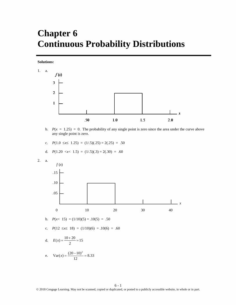
6 - 1 © 2018 Cengage Learning. May not be scanned, copied or duplicated, or posted to a publicly accessible website, in whole or in part.
Chapter 6 Continuous Probability Distributions Solutions: 1. a.
b. P(x = 1.25) = 0. The probability of any single point is zero since the area under the curve above
any single point is zero. c. P(1.0 ≤x≤ 1.25) = (1/.5)(.25) = 2(.25) = .50 d. P(1.20 <x< 1.5) = (1/.5)(.3) = 2(.30) = .60 2. a.
b. P(x< 15) = (1/10)(5) = .10(5) = .50 c. P(12 ≤x≤ 18) = (1/10)(6) = .10(6) = .60
d. 10 20( ) 15
2E x +
= =
e. 2(20 10)Var( ) 8.33
12x −
= =
.15
.10
.05
10 20 30 40
f (x)
x
0

Chapter 6
6 - 2 © 2018 Cengage Learning. May not be scanned, copied or duplicated, or posted to a publicly accessible website, in whole or in part.
4. a.
b. P(.25 <x< .75) = 1 (.50) = .50 c. P(x≤ .30) = 1 (.30) = .30 d. P(x> .60) = 1 (.40) = .40 e./f. Answers will vary.
6. a. For a uniform probability density function
Thus, = .00625.
Solving for , we have = 1/.00625 = 160 In a uniform probability distribution, ½ of this interval is below the mean and ½ of this interval is
above the mean. Thus, a = 136 – ½(160) = 56 and b = 136 + ½(160) = 216 b. c. d.
8.

Continuous Probability Distributions
6 - 3 © 2018 Cengage Learning.May not be scanned, copied or duplicated, or posted to a publicly accessible website, in whole or in part.
10.
These probabilities can be obtained using Excel’s NORM.S.DIST function or the standard normal probability table in the text.
a. P(z≤ 1.5) = .9332 = NORM.S.DIST(1.5,TRUE) b. P(z≤ 1.0) = .8413 = NORM.S.DIST(1,TRUE) c. P(1 ≤z≤ 1.5) = P(z≤ 1.5) - P(z< 1) = .9932 - .8413 = .0919 OR = NORM.S.DIST(1.5,TRUE) - NORM.S.DIST(1,TRUE) = .0918 d. P(0 <z< 2.5) = P(z< 2.5) - P(z≤ 0) = .9938 - .5000 = .4938 OR = NORM.S.DIST(2.5,TRUE) - NORM.S.DIST(0,TRUE) 12. These probabilities can be obtained using Excel’s NORM.S.DIST function or the standard normal
probability table in the text. a. P(0 ≤z≤ .83) = P(z < .83) – P(z < 0) = .7967 - .5000 = .2967 OR = NORM.S.DIST(.83,TRUE) - NORM.S.DIST(0,TRUE) b. P(-1.57 ≤z≤ 0) = P(z < 0) – P(z < -1.57) = .5000 - .0582 = .4418 OR = NORM.S.DIST(0,TRUE) - NORM.S.DIST(-1.57,TRUE) c. P(z> .44) = 1 – P(z < .44) = 1 - .6700 = .3300 = 1 - NORM.S.DIST(.44,TRUE) d. P(z≥ -.23) = 1 – P(z < -.23) = 1 - .4090 = .5910 = 1 - NORM.S.DIST(-.23,TRUE) e. P(z< 1.20) = .8849 = NORM.S.DIST(1.2,TRUE) f. P(z ≤ -.71) = .2389 = NORM.S.DIST(-.71,TRUE) 13. These probabilities can be obtained using Excel’s NORM.S.DIST function or the standard normal
probability table in the text. a. P(-1.98 ≤z≤ .49) = P(z≤ .49) - P(z< -1.98) = .6879 - .0239 = .6640 OR = NORM.S.DIST(.49,TRUE) - NORM.S.DIST(-1.98,TRUE) = .6641 b. P(.52 ≤z≤ 1.22) = P(z≤ 1.22) - P(z< .52) = .8888 - .6985 = .1903 OR = NORM.S.DIST(1.22,TRUE) - NORM.S.DIST(.52,TRUE) c. P(-1.75 ≤z≤ -1.04) = P(z≤ -1.04) - P(z< -1.75) = .1492 - .0401 = .1091 OR = NORM.S.DIST(-1.04,TRUE) - NORM.S.DIST(-1.75,TRUE) 14. These z values can be obtained using Excel’s NORM.S.INV function or by using the standard
normal probability table in the text. a. The z value corresponding to a cumulative probability of .9750 is z = 1.96. = NORM.S.INV(.975) b. Since the area to the left of z=0 is .5, thez value here also corresponds to a cumulative probability of .9750: z = 1.96.NORM.S.INV(.975) c. The z value corresponding to a cumulative probability of .7291 is z = .61. = NORM.S.INV(.7291) d. Area to the left of z is 1 - .1314 = .8686. So z = 1.12. NORM.S.INV(.8686)

Chapter 6
6 - 4 © 2018 Cengage Learning. May not be scanned, copied or duplicated, or posted to a publicly accessible website, in whole or in part.
e. The z value corresponding to a cumulative probability of .6700 is z = .44. NORM.S.INV(.67) f. The area to the left of z is .6700. So z = .44. NORM.S.INV(.67) 15. These z values can be obtained using Excel’s NORM.S.INV function or by using the standard
normal probability table in the text. a. The z value corresponding to a cumulative probability of .2119 is z = -.80. NORM.S.INV(.2119) b. Compute .9030/2 = .4515; z corresponds to a cumulative probability of .5000 + .4515 = .9515. So z
= 1.66. NORM.S.INV(.9515) c. Compute .2052/2 = .1026; z corresponds to a cumulative probability of .5000 + .1026 = .6026. So z
= .26. NORM.S.INV(.6026) d. The z value corresponding to a cumulative probability of .9948 is z = 2.56. NORM.S.INV(.9948) e. The area to the left of z is 1 - .6915 = .3085. So z = -.50. NORM.S.INV(.3085) 16. These z values can be obtained using Excel’s NORM.S.INV function or the standard normal
probability table in the text. a. The area to the left of z is 1 - .0100 = .9900. The z value in the table with a cumulative probability
closest to .9900 is z = 2.33. NORM.S.INV(.99) b. The area to the left of z is .9750. So z = 1.96. NORM.S.INV(.975) c. The area to the left of z is .9500. Since .9500 is exactly halfway between .9495 (z = 1.64) and
.9505(z = 1.65), we select z = 1.645. However, z = 1.64 or z = 1.65 are also acceptable answers. NORM.S.INV(.95)
d. The area to the left of z is .9000. So z = 1.28 is the closest z value. NORM.S.INV(.9) 18. µ = 14.4 and σ = 4.4
a. At x = 20, 20 14.4 1.27
4.4z −
= =
P(z≤ 1.27) = .8980 P(x≥ 20) = P( z > 1.27) = 1 – P(z <1.27) = 1 - .8980 = .1020 Using Excel:1-NORM.DIST(20,14.4,4.4,TRUE) = .1016
b. At x = 10, 10 14.4 1.00
4.4z −
= = −
P(z ≤ -1.00) = .1587 So, P(x≤ 10) = .1587 Using Excel:1-NORM.DIST(10,14.4,4.4,TRUE) = .1587 c. A z-value of 1.28 cuts off an area of approximately 10% in the upper tail.
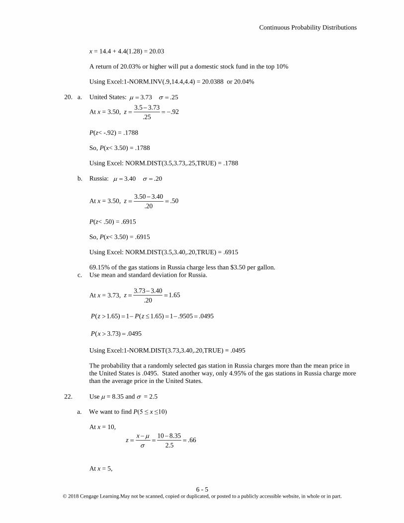
Continuous Probability Distributions
6 - 5 © 2018 Cengage Learning.May not be scanned, copied or duplicated, or posted to a publicly accessible website, in whole or in part.
x = 14.4 + 4.4(1.28) = 20.03 A return of 20.03% or higher will put a domestic stock fund in the top 10% Using Excel:1-NORM.INV(.9,14.4,4.4) = 20.0388 or 20.04% 20. a. United States: 3.73 .25µ σ= =
At x = 3.50, 3.5 3.73 .92.25
z −= = −
P(z< -.92) = .1788 So, P(x< 3.50) = .1788 Using Excel: NORM.DIST(3.5,3.73,.25,TRUE) = .1788 b. Russia: 3.40 .20µ σ= =
At x = 3.50, 3.50 3.40 .50
.20z −
= =
P(z< .50) = .6915 So, P(x< 3.50) = .6915 Using Excel: NORM.DIST(3.5,3.40,.20,TRUE) = .6915 69.15% of the gas stations in Russia charge less than $3.50 per gallon. c. Use mean and standard deviation for Russia.
At x = 3.73, 3.73 3.40 1.65
.20z −
= =
( 1.65) 1 ( 1.65) 1 .9505 .0495P z P z> = − ≤ = − = ( 3.73) .0495P x > = Using Excel:1-NORM.DIST(3.73,3.40,.20,TRUE) = .0495 The probability that a randomly selected gas station in Russia charges more than the mean price in
the United States is .0495. Stated another way, only 4.95% of the gas stations in Russia charge more than the average price in the United States.
22. Use µ = 8.35 and σ = 2.5
a. We want to find P(5 ≤ x ≤10) At x = 10,
10 8.35 .66
2.5xz µ
σ− −
= = =
At x = 5,

Chapter 6
6 - 6 © 2018 Cengage Learning. May not be scanned, copied or duplicated, or posted to a publicly accessible website, in whole or in part.
5 8.35 1.342.5
xz µσ− −
= = = −
P(5 ≤ x ≤ 10) = P(-1.34 ≤ z ≤ .66)= P(z ≤ .66) - P(z ≤ -1.34) = .7454 - .0901 = .6553 Using Excel: NORM.DIST(10,8.35,2.5,TRUE) – NORM.DIST(5,8.35,2.5,TRUE) = .6553 The probability of a household viewing television between 5 and 10 hours a day is .6553.
b. Find the z-value that cuts off an area of .03 in the upper tail. Using a cumulative probability of 1 - .03 = .97, z = 1.88 provides an area of .03 in the upper tail of the normal distribution.
x = µ + zσ = 8.35 + 1.88(2.5) = 13.05 hours Using Excel: NORM.INV(.97,8.35,2.5) = 13.0520
A household must view slightly over 13 hours of television a day to be in the top 3% of television viewing households.
c. At x = 3, 3 8.35 2.14
2.5xz µ
σ− −
= = = −
P(x>3) = P(z > -2.14) = 1 - P(z< -2.14) = 1 - .0162 = .9838 Using Excel:1-NORM.DIST(3,8.35,2.5) = .9838 The probability a household views more than 3 hours of television a day is .9838.
24. µ = 749 and σ = 225
a.
P = P = .0606 The probability that expenses will be less than $400 is .0606. Using Excel: NORM.DIST(400,749,225,TRUE) = .0604
b.
P = P = 1 P = 1 - .5910 = .4090 The probability that expenses will be $800 or more is .4090. Using Excel:1-NORM.DIST(800,749,225,TRUE) = .4103
c. For x = 1000,
Continuous Probability Distributions
6 - 7 © 2018 Cengage Learning.May not be scanned, copied or duplicated, or posted to a publicly accessible website, in whole or in part.
For x = 500,
P(500 x 1000) = P(-1.11 < z < 1.12) = P P = .8686 .1335 = .7351 The probability that expenses will be between $500 and $1000 is .7351. Using Excel: NORM.DIST(1000,749,225,TRUE) – NORM.DIST(500,749,225,TRUE) = .7335 d. The upper 5%, or area = occurs for x zµ σ= + = 749 + 1.645(225) = $1119 The 5% most expensive travel plans will be slightly more than $1119 or higher. Using Excel: NORM.INV(.95,749,225) = 1119.0921
26. µ = 8 a. P(x≤ 6) = 1 - e-6/8 = 1 - .4724 = .5276
Using Excel: EXPON.DIST(6,1/8,TRUE) = .5276 b. P(x≤ 4) = 1 - e-4/8 = 1 - .6065 = .3935
Using Excel: EXPON.DIST(4,1/8,TRUE) = .3935 c. P(x≥ 6) = 1 - P(x≤ 6) = 1 - .5276 = .4724 Using Excel: =1-EXPON.DIST(6,1/8,TRUE) = .4724 d. P(4 ≤x≤ 6) = P(x≤ 6) - P(x≤ 4) = .5276 - .3935 = .1342
Using Excel: EXPON.DIST(6,1/8,TRUE)-EXPON.DIST(4,1/8,TRUE) = .1342 27. µ = 3 a. 0 / 3
0( ) 1 xP x x e−≤ = − b. P(x≤ 2) = 1 - e-2/3 = 1 - .5134 = .4866
Using Excel: EXPON.DIST(2,1/3,TRUE) = .4866 c. P(x≥ 3) = 1 - P(x≤ 3) = 1 - (1 - e−3 3/ ) = e-1 = .3679 Using Excel: =1-EXPON.DIST(3,1/3,TRUE) = .3679 d. P(x≤ 5) = 1 - e-5/3 = 1 - .1889 = .8111 Using Excel: EXPON.DIST(5,1/3,TRUE) = .8111 e. P(2 ≤x≤ 5) = P(x≤ 5) - P(x≤ 2) = .8111 - .4866 = .3245 Using Excel: EXPON.DIST(5,1/3,TRUE)-EXPON.DIST(2,1/3,TRUE) = .3245

Chapter 6
6 - 8 © 2018 Cengage Learning. May not be scanned, copied or duplicated, or posted to a publicly accessible website, in whole or in part.
28. a. Withµ = 20, /201( )20
xf x e−=
b. P(x ≤ 15) =
/ 15/201 1xe eµ− −− = − = .5276 =EXPON.DIST(15,1/20,TRUE) c. P( x> 20) = 1 - P(x ≤ 20)
= 1 - (1 -20/20e−
) = 1 .3679e− = =1 - EXPON.DIST(20,1/20,TRUE)
d. Withµ = 7, /71( )7
xf x e−=
/ 5/7( 5) 1 1 .5105xP x e eµ− −≤ = − = − = =EXPON.DIST(5,1/7,TRUE)
29. a.
µ = 12 b. P(x≤ 12) = 1 - e-12/12 = 1 - .3679 = .6321
Using Excel: EXPON.DIST(12,1/12,TRUE) = .6321 c. P(x≤ 6) = 1 - e-6/12 = 1 - .6065 = .3935
Using Excel: EXPON.DIST(6,1/12,TRUE) = .3935 d. P(x≥ 30) = 1 - P(x< 30) = 1 - (1 - e-30/12) = .0821 Using Excel: =1-EXPON.DIST(30,1/12,TRUE) = .0821 30. µ = 2
a. / /21 1( )2
x xf x e eµ
µ− −= = for x> 0
Continuous Probability Distributions
6 - 9 © 2018 Cengage Learning.May not be scanned, copied or duplicated, or posted to a publicly accessible website, in whole or in part.
P(x<x0) = 0 /1 xe µ−− P(x< 1) = 1/21 e−− = .51 e−− = 1 - .6065 = .3935 =EXPON.DIST(1,1/2,TRUE) b. P(x< 2) = 2/21 e−− = 1.01 e−− = 1 - .3679 = .6321 (1 2) ( 2) ( 1)P x P x P x≤ ≤ = ≤ − ≤ = .6321 - .3935 = .2386 =EXPON.DIST(2,1/2,TRUE) – EXPON.DIST(1,1/2,TRUE) = .2387
c. For this customer, the cable service repair would have to take longer than 4 hours.
( 4) 1 ( 4)P x P x> = − ≤ = 1 4/2 2.0(1 ) .1353e e− −− − = = =1 - EXPON.DIST(4,1/2,TRUE) 32. a. Because the number of calls per hour follows a Poisson distribution, the time between calls follows
an exponential distribution. So, for a mean of 1.6 calls per hour, the mean time between calls is
per call
b. The exponential probability density function is f (x) = for
where x is the minutes between 911 calls. c. Using time in minutes, = EXPON.DIST(60, 1/ 37.5,TRUE) d. = 1- EXPON.DIST(30, 1/ 37.5,TRUE) e. ( ) 20/37.5 5/37.55 20 (1 ) (1 ) .4134 .1248 .2885P x e e−≤ ≤ = − − − = − = EXPON.DIST(20, 1/ 37.5,TRUE - EXPON.DIST(5, 1/ 37.5,TRUE) = .2885 34. μ = 19000 and σ = 2100 a. Find the z value that cuts off an area of .10 in the lower tail. From the standard normal table z≈ -1.28. Solve for x,
19,0001.282100
xz −= − =
x = 19,000 – 1.28(2100) = 16,312 10% of athletic scholarships are valued at $16,312 or less. Using Excel: NORM.INV(.90,19000,2100) = 16,308.74
Chapter 6
6 - 10 © 2018 Cengage Learning. May not be scanned, copied or duplicated, or posted to a publicly accessible website, in whole or in part.
b. 22,000 19,000 1.432100
xz µσ− −
= = =
P(x≥ 22,000) = P( z > 1.43) = 1 – P(z≤ 1.43) = 1 - .9236 = .0764 7.64% of athletic scholarships are valued at $22,000 or more. Using Excel:1-NORM.DIST(22000,19000,2100,TRUE) = .0766 c. Find the z value that cuts off an area of .03 in the upper tail: z = 1.88. Solve for x,
19,0001.882100
xz −= =
x = 19,000 + 1.88(2100) = 22,948 3% of athletic scholarships are valued at $22,948 or more. Using Excel: NORM.INV(.97,19000,2100) = 22,949.6666 36. µ = 658 a. z = -1.88 cuts off .03 in the lower tail So,
610 6581.88z
σ−
= − =
610 658 25.5319
1.88σ −
= =−
Using EXCEL: NORM.S.INV(.03), z = -1.8807936, solving for σ without rounding, gives 25.5211
b. At 700, 700 658 1.6525.5319
xz µσ− −
= = =
At 600, 600 659 2.3125.5319
xz µσ− −
= = = −
P(600 <x< 700) =P(-2.31 <z< 1.65) = P(z < 1.65) – P(z < -2.31) = .9505 - .0104 = .9401 Using Excel: NORM.DIST(700,658,25.5211,TRUE) –NORM.DIST(600,658,25.5211,TRUE) = .9386 c. z = 1.88 cuts off approximately .03 in the upper tail x = 658 + 1.88(25.5319) = 706. Using Excel: NORM.INV(.97,658,25.5211) = 706
On the busiest 3% of days 706 or more people show up at the pawnshop.

Continuous Probability Distributions
6 - 11 © 2018 Cengage Learning.May not be scanned, copied or duplicated, or posted to a publicly accessible website, in whole or in part.
38. a. At x = 200 200 150 2
25z −
= =
P(x> 200) = P(z> 2) = 1 - P(z≤ 2) = 1 - .9772 = .0228= 1- NORM.DIST(200,150,25,TRUE) b. Expected Profit = Expected Revenue - Expected Cost = 200 - 150 = $50 40. μ = 450 and σ = 100 a. At 400,
400 450 .500100
z −= = −
Area to left is .3085 At 500,
500 450 .500100
z −= = +
Area to left is .6915 P(400 ≤x ≤ 500) = P(-.5 < z < .5) = P(z < .5) – P(z < -.5) = .6915 - .3085 = .3830
Using Excel: NORM.DIST(500,450,100,TRUE) - NORM.DIST(400,450,100,TRUE) = .3829
38.3% will score between 400 and 500. b. At 630,
630 450 1.80100
z −= =
Probability of worse than 630 = P( x < 630) = P(z < 1.8) =.9641 Using Excel: NORM.DIST(630,450,100,TRUE) = .9641 Probability of better than 630 = P( x > 630) = P(z > 1.8) =1- P(z < 1.8) = 1 - .9641 = .0359 Using Excel: 1 - NORM.DIST(630,450,100,TRUE) = 1 - .9641 = .0359 96.41% do worse and 3.59% do better . c. At 480,
480 450 .30100
z −= =
Area to left is .6179 Probability of admittance = P( x > 480) = P(z >.3) =1- P(z <.3) = 1 - .6179 = .3821 Using Excel: 1 - NORM.DIST(480,450,100,TRUE) = 1 - .6179 = .3821 38.21% are acceptable.

Chapter 6
6 - 12 © 2018 Cengage Learning. May not be scanned, copied or duplicated, or posted to a publicly accessible website, in whole or in part.
42. σ= .6 At 2%
z≈ -2.05 x = 18
xz µσ−
=182.05
.6µ−
∴− =
µ = 18 + 2.05 (.6) = 19.23 oz.
The mean filling weight must be 19.23 oz. 44. a. Mean time between arrivals = 1/7 minutes b. f(x) = 7e-7x c. P(no one in 1 minute) = P(greater than 1 minute between arrivals) = P(x> 1) = 1 - P(x< 1) = 1 - [1 - e-7(1)] = e-7 = .0009 =1 - EXPON.DIST(1,1/(1/7),TRUE) = 1-EXPON.DIST(1,7,TRUE) = .0009 Note using Poisson via Excel gives: POISSON.DIST(0,7,TRUE) = .0009 d. 12 seconds is .2 minutes, or 1/5 of a minute, therefore poisson mean = 7/5 per 12 seconds = 1.4 Using exponential, P(no one in 12 seconds = P(greater than 12 seconds between arrivals) = P(x> .2) = 1 - P(x< .2) = 1- [1- e-7(.2)] = e-1.4 = .2466 =1 - EXPON.DIST(.2,1/(1/7),TRUE) = 1-EXPON.DIST(.2,7,TRUE) = .2466 Note using Poisson via Excel gives: POISSON.DIST(0,7/5,TRUE) = .2466
46. a. 1 05µ
= . therefore µ = 2 minutes = mean time between telephone calls
b. Note: 30 seconds = .5 minutes P(x≤ .5) = 1 - e-.5/2 = 1 - .7788 = .2212=EXPON.DIST(.5,1/2,TRUE) c. P(x≤ 1) = 1 - e-1/2 = 1 - .6065 = .3935=1 - EXPON.DIST(1,1/2,TRUE) d. P(x≥ 5) = 1 - P(x< 5) = 1 - (1 - e-5/2) = .0821=1 - EXPON.DIST(5,1/2,TRUE)

7 - 1 © 2018 Cengage Learning.May not be scanned, copied or duplicated, or posted to a publicly accessible website, in whole or in part.
Chapter 7 Sampling and Sampling Distributions Solutions: 1. a. AB, AC, AD, AE, BC, BD, BE, CD, CE, DE b. With 10 samples, each has a 1/10 probability. c. B and D because the two smallest random numbers are .0476 and .0957. 2. The 4 smallest random numbers are .0341, .0729, .0936, and .1449. So elements 2, 3, 5, and 10 are
the simple random sample. 3. The simple random sample consists of New York, Detroit, Oakland, Boston, and Kansas City. 4. Step 1: Generate a random number using the RAND() function for each of the 10 golfers. Step 2: Sort the list of golfers with respect to the random numbers. The first 3 golfers in the sorted
list make up the simple random sample. Answers will vary with every regeneration of random numbers.
6. a. Finite population.A frame could be constructed obtaining a list of licensed drivers from the New
York state driver’s license bureau. b. Sampling from an infinite population. The sample is taken from the production line producing boxes
of cereal. c. Sampling from an infinite population. The sample is taken from the ongoing arrivals to the Golden
Gate Bridge. d. Finite population.A frame could be constructed by obtaining a listing of students enrolled in the
course from the professor. e. Sampling from an infinite population. The sample is taken from the ongoing orders being processed
by the mail-order firm.
7. a. x x ni= = =Σ / 546
9
b. s x xn
i=−−
Σ( )2
1
Σ( )x xi − 2 =(-4)2 + (-1)2 + 12+ (-2)2 + 12 + 52=48
s = 486 1
31−
= .

Chapter 7
7 - 2 © 2018 Cengage Learning. May not be scanned, copied or duplicated, or posted to a publicly accessible website, in whole or in part.
8. a. p =75/150=.50 b. p =55/150=.3667
9. a. x x ni= = =Σ / 4655
93
b.
xi ( )x xi − ( )x xi − 2 94 +1 1 100 +7 49 85 -8 64 94 +1 1 92 -1 1 Totals 465 0 116
s x xn
i=−−
= =Σ( )
.2
1116
4539
10. a. Two of the 40 stocks in the sample received a 5 Star rating.
2 .0540
p = =
b. Seventeen of the 40 stocks in the sample are rated Above Average with respect to risk.
17 .42540
p = =
c. There are eight stocks in the sample that are rated 1 Star or 2 Star.
8 .2040
p = =
12. a. The sampled population is U. S. adults that are 50 years of age or older. b. We would use the sample proportion for the estimate of the population proportion.
350 .8216426
p = =
c. The sample proportion for this issue is .74 and the sample size is 426. The number of respondents citing education as “very important” is (.74)*426 = 315. d. We would use the sample proportion for the estimate of the population proportion.
354 .8310426
p = =
e. The inferences in parts (b) and (d) are being made about the population of U.S. adults who are age 50or older.So, the population of U.S. adults who are age 50 or older is the target population.The target population is the same as the sampled population.If the sampled population was

Sampling and Sampling Distributions
7 - 3 © 2018 Cengage Learning.May not be scanned, copied or duplicated, or posted to a publicly accessible website, in whole or in part.
restrictedtomembers of AARP who were 50 years of age or older, the sampled population would not be the same as the target population.The inferences made in parts (b) and (d) would only be valid ifthe population of AARP members age 50 or older was representative of the U.S. population ofadults age 50 and over.
14. a. Use the data disk accompanying the book and the EAI file.Generate a random number for each
manager and select managers associated with the 50 smallest random numbers as the sample. Answers will vary with every regeneration of random numbers.
b. Use Excel's AVERAGE function to compute the mean for the sample. c. Use Excel's STDEV.S function to compute the sample standard deviation. d. Use the sample proportion as a point estimate of the population proportion. 15. a. The sampling distribution is normal with E ( )x = µ = 200 / 50 / 100 5x nσ σ= = = For ± 5,195 205x≤ ≤ Using Standard Normal Probability Table:
At x = 205, 5
15x
xz
µ
σ
−= = = ( 1)P z ≤ = .8413
At x = 195, 5 15x
xz µσ− −
= = = − ( 1)P z < − = .1587
(195 205)P x≤ ≤ = .8413 - .1587 = .6826 Using Excel:NORM.DIST(205,200,50/SQRT(100),TRUE) - NORM.DIST(195,200,50/SQRT(100),TRUE)=.6827 b. For ± 10, 190 210x≤ ≤ Using Standard Normal Probability Table:
At x = 210, z x
x
=−
= =µ
σ105
2 ( 2)P z ≤ = .9772
At x = 190,10
25x
xz
µ
σ
− −= = = − ( 2)P z < − = .0228
(190 210)P x≤ ≤ = .9772 - .0228 = .9544 Using Excel: NORM.DIST(210,200,50/SQRT(100),TRUE) - NORM.DIST(190,200,50/SQRT(100),TRUE)=.9545

Chapter 7
7 - 4 © 2018 Cengage Learning. May not be scanned, copied or duplicated, or posted to a publicly accessible website, in whole or in part.
x
16. σ σx n= / 25 / 50 3.54xσ = = For sample size = 100, 25 / 100 2.50xσ = = For sample size = 150, 25 / 150 2.04xσ = = For sample size = 200, 25 / 200 1.77xσ = = The standard error of the mean decreases as the sample size increases. 18. a.
( )E x The normal distribution for x is based on the Central Limit Theorem. b. For n = 120, E ( x ) remains $51,800 and the sampling distribution of x can still be approximated by
a normal distribution.However, σ x is reduced to 4000 120/ = 365.15. c. As the sample size is increased, the standard error of the mean, xσ , is reduced.This appears logical
from the point of view that larger samples should tend to provide sample means that are closer to the population mean.Thus, the variability in the sample mean, measured in terms of xσ , should decrease as the sample size is increased.
19. a. With a sample of size 60 4000 516.4060xσ = =
At x = 52,300, 52,300 51,800 .97516.40
z −= =
P( x ≤ 52,300) = P(z ≤ .97) = .8340
At x = 51,300, 51,300 51,800 .97516.40
z −= = −
/ 4000 / 60 516.40x nσ σ= = =

Sampling and Sampling Distributions
7 - 5 © 2018 Cengage Learning.May not be scanned, copied or duplicated, or posted to a publicly accessible website, in whole or in part.
P( x < 51,300) = P(z < -.97) = .1660 P(51,300 ≤ x ≤ 52,300) = .8340 - .1660 = .6680 Using Excel: NORM.DIST(52300,51800,4000/SQRT(60),TRUE)- NORM.DIST(51300,51800,4000/SQRT(60),TRUE)=.6671 20. a. Normal distribution, ( ) 17.5E x µ= = / 4 / 50 .5657x nσ σ= = = b. Within 1 week means 16.5 ≤ x ≤18.5
At x = 18.5, 18.5 17.5 1.77.5657
z −= = .P(z ≤ 1.77) = .9616
At x = 16.5, z = -1.77. P(z < -1.77) = .0384 So P(16.5 ≤ x ≤ 18.5) = .9616 - .0384 = .9232 Using Excel: NORM.DIST(18.5,17.5,4/SQRT(50),TRUE) - NORM.DIST(16.5,17.5,4/SQRT(50),TRUE) = .9229 c. Within 1/2 week means 17.0 ≤ x ≤ 18.0
At x = 18.0, 18.0 17.5 .88.5657
z −= = . P(z ≤ .88) = .8106
At x = 17.0, z = -.88. P(z < -.88) = .1894 P(17.0 ≤ x ≤ 18.0) = .8106 - .1894 = .6212 Using Excel: NORM.DIST(18,17.5,4/SQRT(50),TRUE) - NORM.DIST(16,17.5,4/SQRT(50),TRUE) = .6232
22. a. 16642/
xznσ
−=
Within ± 200 means x - 16,642 must be between -200 and +200. The z value for x - 16,642 = -200 is the negative of the z value for x - 16,642 = 200.So we just
show the computation of z for x - 16,642 = 200.
n = 30 200 .462400 / 30
z = = P(-.46 ≤ z ≤ .46) = .6772 - .3228 = .3544
Using Excel: NORM.DIST(16842,16642,2400/SQRT(30),TRUE)- NORM.DIST(16442,16642,2400/SQRT(30),TRUE) = .3519
n = 50 200 .592400 / 50
z = = P(-.59 ≤ z ≤ .59) = .7224 - .2776 = .4448

Chapter 7
7 - 6 © 2018 Cengage Learning. May not be scanned, copied or duplicated, or posted to a publicly accessible website, in whole or in part.
Using Excel: NORM.DIST(16842,16642,2400/SQRT(50),TRUE)- NORM.DIST(16442,16642,2400/SQRT(50),TRUE) = .4443
n = 100 200 .832400 / 100
z = = P(-.83 ≤ z ≤ .83) = .7967 - .2033 = .5934
Using Excel: NORM.DIST(16842,16642,2400/SQRT(100),TRUE)- NORM.DIST(16442,16642,2400/SQRT(100),TRUE) = .5953
n = 400 200 1.672400 / 400
z = = P(-.1.67 ≤ z ≤ .1.67) = .9525 - .0475 = .9050
Using Excel: NORM.DIST(16842,16642,2400/SQRT(400),TRUE)- NORM.DIST(16442,16642,2400/SQRT(400),TRUE) = .9044 b. A larger sample increases the probability that the sample mean will be within a specified
distance of the population mean.In this instance, the probability of being within ±200 of µ ranges from .3544 for a sample of size 30 to .9050 for a sample of size 400.
24. a. This is a graph of a normal distribution with ( )E x =µ= 22 and / 4 / 30 .7303x nσ σ= = = b. Within 1 inch means 21 ≤ x ≤ 23
23 22 1.37.7303
z −= = 21 22 1.37
.7303z −
= = −
P(21 ≤ x ≤ 23) = P(–1.37 ≤ z ≤ 1.37) = .9147 – .0853 = .8294 The probability the sample mean will be within 1 inch of the population mean of 22 is .8294. Using Excel: NORM.DIST(23,22,4/SQRT(30),TRUE)- NORM.DIST(21,22,4/SQRT(30),TRUE) = .8291 c. / 4 / 45 .5963x nσ σ= = = Within 1 inch means 41 ≤ x ≤43
43 42 1.68.5963
z −= = 41 42 1.68
.5963z −
= = −
P(41 ≤ x ≤ 43) = P(–1.68 ≤ z ≤ 1.68) = .9535 – .0465 = .9070 The probability the sample mean will be within 1 inch of the population mean of 42 is .9070. Using Excel: NORM.DIST(43,42,4/SQRT(45),TRUE)- NORM.DIST(41,42,4/SQRT(45),TRUE) = .9065 d. The probability of being within 1 inch is greater for New York in part (c) because the sample size is
larger.
Sampling and Sampling Distributions
7 - 7 © 2018 Cengage Learning.May not be scanned, copied or duplicated, or posted to a publicly accessible website, in whole or in part.
26. a. n / N = 40 / 4000 = .01 < .05; therefore, the finite population correction factor is not necessary. b. With the finite population correction factor
σσ
xN nN n
=−−
=−−
=1
4000 404000 1
8 240
129. .
Without the finite population correction factor / 8.2 / 40 1.30x nσ σ= = = Including the finite population correction factor provides only a slightly different value for σ x than
when the correction factor is not used. c. Even though the population mean is not given, stating “within +2” equates to “ x µ− ”.
2 2 1.541.30/ 8.2 / 40
xzn
µσ
− ± ±= = = = ± P(z ≤ 1.54) = .9382
P(z < -1.54) = .0618 Probability = .9382 - .0618 = .8764 Using Excel: No value for the population mean is given, but we can use Excel’s NORM.S.DIST function here. NORM.S.DIST(2/(8.2/SQRT(40)),TRUE)-NORM.S.DIST(-2/(8.2/SQRT(40)),TRUE) =.8771 28. a. E( p ) = p= .40
(1 ) .40(.60) .0346200p
p pn
σ −= = =
Within ± .03 means .37 ≤ p ≤ .43
.03 .87.0346p
p pzσ−
= = = P(z ≤ .87) = .8078
P(z< -.87) = .1922 P(.37 ≤ p ≤ .43) = .8078 - .1922 = .6156 Using Excel:NORM.DIST(.43,.40,SQRT(.4*.6/200),TRUE)- NORM.DIST(.37,.40,SQRT(.4*.6/200),TRUE) = .6135
b. .05 1.44.0346p
p pzσ−
= = = P(z ≤ 1.44) = .9251
P(z< -1.44) = .0749
Chapter 7
7 - 8 © 2018 Cengage Learning. May not be scanned, copied or duplicated, or posted to a publicly accessible website, in whole or in part.
P(.35 ≤ p ≤ .45) = .9251 - .0749 = .8502 Using Excel:NORM.DIST(.45,.40,SQRT(.4*.6/200),TRUE)- NORM.DIST(.35,.40,SQRT(.4*.6/200),TRUE)=.8511 30. E( p ) = p = .30
a. (.30)(.70) .0458100pσ = =
Within ± .04 means .26 ≤ p ≤ .34
.04 .87.0458p
p pzσ−
= = = P(z ≤ .87) = .8078
P(z< -.87) = .1922 P(.26 ≤ p ≤ .34) = .8078 - .1922 = .6156 Using Excel:NORM.DIST(.34,.30,SQRT(.3*.7/100),TRUE) - NORM.DIST(.26,.30,SQRT(.3*.7/100),TRUE)=.6173
b. (.30)(.70) .0324200pσ = =
.04 1.23.0324p
p pzσ−
= = = P(z ≤ 1.23) = .8907
P(z< -1.23) = .1093 P(.26 ≤ p ≤ .34) = .8907 - .1093 = .7814 Using Excel:NORM.DIST(.34,.30,SQRT(.3*.7/200),TRUE) - NORM.DIST(.26,.30,SQRT(.3*.7/200),TRUE)=.7830
c. (.30)(.70) .0205500pσ = =
.04 1.95.0205p
p pzσ−
= = = P(z ≤ 1.95) = .9744
P(z< -1.95) = .0256 P(.26 ≤ p ≤ .34) = .9744 - .0256 = .9488 Using Excel:NORM.DIST(.34,.30,SQRT(.3*.7/500),TRUE) - NORM.DIST(.26,.30,SQRT(.3*.7/500),TRUE)=.9490
d. (.30)(.70) .01451000pσ = =

Sampling and Sampling Distributions
7 - 9 © 2018 Cengage Learning.May not be scanned, copied or duplicated, or posted to a publicly accessible website, in whole or in part.
.04 2.76.0145p
p pzσ−
= = = P(z ≤ 2.76) = .9971
P(z< -2.76) = .0029 P(.26 ≤ p ≤ .34) = .9971 - .0029 = .9942 Using Excel:NORM.DIST(.34,.30,SQRT(.3*.7/1000),TRUE) - NORM.DIST(.26,.30,SQRT(.3*.7/1000),TRUE)=.9942 e. With a larger sample, there is a higher probability p will be within ± .04 of the population
proportion p. 31. a.
The normal distribution is appropriate because np = 100(.30) = 30 and n(1 - p) = 100(.70) = 70 are both greater than 5.
b. P (.20 ≤ p ≤ .40) = ?
.40 .30 2.18.0458
z −= = P(z ≤ 2.18) = .9854
P(z< -2.18) = .0146 P(.20 ≤ p ≤ .40) = .9854 - .0146 = .9708 Using Excel:NORM.DIST(.40,.30,SQRT(.3*.7/100),TRUE) - NORM.DIST(.20,.30,SQRT(.3*.7/100),TRUE)=.9709 c. P (.25 ≤ p ≤ .35) = ?
.35 .30 1.09.0458
z −= = P(z ≤ 1.09) = .8621
P(z< -1.09) = .1379 P(.25 ≤ p ≤ .35) = .8621 - .1379 = .7242 Using Excel:NORM.DIST(.35,.30,SQRT(.3*.7/100),TRUE) -
(1 ) .30(.70) .0458100p
p pn
σ −= = =
p
Chapter 7
7 - 10 © 2018 Cengage Learning. May not be scanned, copied or duplicated, or posted to a publicly accessible website, in whole or in part.
NORM.DIST(.25,.30,SQRT(.3*.7/100),TRUE)=.7248 32. a. This is a graph of a normal distribution with a mean of ( )E p = p= .55 and
(1 ) .55(1 .55) .0352200p
p pn
σ − −= = =
The normal distribution is appropriate because np = 200(.55) = 110 and n(1 - p) = 200(.45) = 90 are both greater than 5. b. Within ± .05 means .50 ≤ p ≤ .60
.60 .55 1.42
.0352p
p pzσ− −
= = = .50 .55 1.42
.0352p
p pzσ− −
= = = −
P(.50 ≤ p ≤ .60) = P(-1.42 ≤ z ≤ 1.42) = .9222 - .0778 = .8444 Using Excel: NORM.DIST(.60,.55,SQRT(.55*.45/200),TRUE)- NORM.DIST(.50,.55,SQRT(.55*.45/200),TRUE) = .8448 c. This is a graph of a normal distribution with a mean of ( )E p = p= .45 and
(1 ) .45(1 .45) .0352200p
p pn
σ − −= = =
The normal distribution is appropriate because np = 200(.45) = 90 and n(1 - p) = 200(.55) = 110 are both greater than 5.
d. (1 ) .45(1 .45) .0352200p
p pn
σ − −= = =
Within ± .05 means .40 ≤ p ≤ .50
.50 .45 1.42.0352p
p pzσ− −
= = = .40 .45 1.42
.0352p
p pzσ− −
= = = −
P(.40 ≤ p ≤ .50) = P(-1.42 ≤ z ≤ 1.42) = .9222 - .0778 = .8444 Using Excel: NORM.DIST(.50,.45,SQRT(.45*.55/200),TRUE) - NORM.DIST(.40,.45,SQRT(.45*.55/200),TRUE) = .8448 e. No, the probabilities are exactly the same.This is because pσ , the standard error, and the width of
the interval are the same in both cases.Notice the formula for computing the standard error.It involves p(1 -p).So wheneverp(1 -p)does not change, the standard error will be the same.In part (b), p = .55 and 1 – p = .45.In part (d), p = .45 and 1 – p = .55.

Sampling and Sampling Distributions
7 - 11 © 2018 Cengage Learning.May not be scanned, copied or duplicated, or posted to a publicly accessible website, in whole or in part.
f. For n = 400, (1 ) .55(1 .55) .0249400p
p pn
σ − −= = =
Within ± .05 means .50 ≤ p ≤ .60
.60 .55 2.01
.0249p
p pzσ− −
= = = .50 .55 2.01
.0249p
p pzσ− −
= = = −
P(.50 ≤ p ≤ .60) = P(-2.01 ≤ z ≤ 2.01) = .9778 - .0222 = .9556 Using Excel NORM.DIST(.60,.55,SQRT(.55*.45/400),TRUE) - NORM.DIST(.50,.55,SQRT(.55*.45/400),TRUE) = .9556 The probability is larger than in part (b).This is because the larger sample size has reduced the
standard error from .0352 to .0249. 34. a. It is a normal distribution withE( p ) = p = .42 and
(1 ) (.42)(.58) .0285300p
p pn
σ −= = =
The normal distribution is appropriate because np = 300(.42) = 126 and n(1 - p) = 300(.58) = 174 are both greater than 5.
b. .03 1.05
.0285p
p pzσ−
= = = P(z ≤ 1.05) = .8531
P(z< -1.05) = .1469 P(.39 ≤ p ≤ .45) = .8531 - .1469 = .7062 Using Excel: NORM.DIST(.45,.42,SQRT(.42*.58/300),TRUE) - NORM.DIST(.39,.42,SQRT(.42*.58/300),TRUE) = .7076
c. .05 1.75
.0285p
p pzσ−
= = = P(z ≤ 1.75) = .9599
P(z< -1.75) = .0401 P(.37 ≤ p ≤ .47) = .9599 - .0401 = .9198 Using Excel: NORM.DIST(.47,.42,SQRT(.42*.58/300),TRUE) - NORM.DIST(.37,.42,SQRT(.42*.58/300),TRUE) = .9207 d. The probabilities would increase.This is because the increase in the sample size makes the
standarderror, pσ , smaller. 36. a. E ( p ) = p= .76
(1 ) .76(1 .76) .0214400p
p pn
σ − −= = =

Chapter 7
7 - 12 © 2018 Cengage Learning. May not be scanned, copied or duplicated, or posted to a publicly accessible website, in whole or in part.
Normal distribution because np = 400(.76) = 304 and n(1 - p) = 400(.24) = 96
b. .79 .76 1.40.0214
z −= = P(z ≤1.40) = .9192
P(z< -1.40) = .0808 P(.73 ≤ p ≤.79) = P(-1.40 ≤z≤ 1.40) = .9192 - .0808 = .8384 Using Excel:NORM.DIST(.79,.76,SQRT(.76*.24/100),TRUE) – NORM.DIST(.73,.76,SQRT(.76*.24/100),TRUE)=.8399
c. (1 ) .76(1 .76) .0156750p
p pn
σ − −= = =
.79 .76 1.92.0156
z −= = P(z ≤ 1.92) = .9726
P(z< -1.92) = .0274 P(.73 ≤ p ≤.79) = P(-1.92 ≤z≤ 1.92) = .9726 - .0274 = .9452 Using Excel:NORM.DIST(.79,.76,SQRT(.76*.24/750),TRUE) – NORM.DIST(.73,.76,SQRT(.76*.24/750),TRUE)=.9456 38. a.
( )E x The normal distribution for x is based on the Central Limit Theorem. For n = 50,
𝐸𝐸(��𝑥) remains 30,𝜎𝜎𝑥𝑥is 6 √50⁄ = 0.8485, and the sampling distribution of ��𝑥can be approximated by a normal distribution.
b.
/ 6 / 50 .8485x nσ σ= = =

Sampling and Sampling Distributions
7 - 13 © 2018 Cengage Learning.May not be scanned, copied or duplicated, or posted to a publicly accessible website, in whole or in part.
( )E x
The normal distribution for x is based on the Central Limit Theorem. For n = 500000, 𝐸𝐸(��𝑥) remains 30 and the sampling distribution of ��𝑥can be approximated by a normal distribution. However, now 𝜎𝜎𝑥𝑥 is 6 √500000⁄ = 0.0085.
c. When the sample size is extremely large, the standard error of the sampling distribution of ��𝑥
becomes very small. This is logical because larger samples tend to provide sample means that are closer to the population mean. Thus, the variability in the sample mean, measured in terms of 𝜎𝜎𝑥𝑥 , should decrease as the sample size is increased and should become very small when the sample size is extremely large.
40. a. 𝐸𝐸(��𝑝) = .37 and 𝜎𝜎𝑝𝑝 = �𝑝𝑝(1 − 𝑝𝑝) 𝑛𝑛⁄ = .0279. ��𝑝 is also approximately normal because 𝑛𝑛𝑝𝑝 = 111 ≥
5 and 𝑛𝑛(1 − 𝑝𝑝) = 189 ≥ 5.
b. At ��𝑝= .32, .32 .37 1.79
.0279z −
= = −
P(��𝑝≤ .32) = P(z ≤ -1.79) = .0367
At��𝑝 =.42, .42 .37 1.79
.0279z −
= =
P(��𝑝<.42) = P(z <1.79) = .9633 P(.42 ≤��𝑝≤ .32) = .9633 - .0367 = .9266 Using Excel: NORM.DIST(.42,.37,SQRT(.37*.63/300),TRUE)- NORM.DIST(.32,.37,SQRT(.37*.63/300),TRUE) = .9271 c. 𝐸𝐸(��𝑝) = .37 and 𝜎𝜎𝑝𝑝 = �𝑝𝑝(1 − 𝑝𝑝) 𝑛𝑛⁄ = .0028. ��𝑝 is also approximately normal because 𝑛𝑛𝑝𝑝 =
11,100 ≥ 5 and 𝑛𝑛(1 − 𝑝𝑝) = 18,900 ≥ 5.
d. At��𝑝= .32, .32 .37 17.94
.0028z −
= = −
P(��𝑝≤ .32) = P(z ≤ -17.94) ≈ .0000
/ 6 / 500000 .0085x nσ σ= = =

Chapter 7
7 - 14 © 2018 Cengage Learning. May not be scanned, copied or duplicated, or posted to a publicly accessible website, in whole or in part.
At��𝑝 =.42, .42 .37 17.94
.0028z −
= =
P(��𝑝<.42) = P(z <17.94) ≈ 1.0000 P(.32 ≤��𝑝≤ .42) ≈ 1.0000 - .0000 = 1.0000 Using Excel: NORM.DIST(.42,.37,SQRT(.37*.63/30000),TRUE)- NORM.DIST(.32,.37,SQRT(.37*.63/30000),TRUE) = 1.0000 e. The probability in part (d) is greater than the probability in part (b) because the lager sample size in
part (d) results in a smaller standard error. 42. a. Sorting the list of companies and random numbers to identify the five companies associated with the
five smallest random numbers provides the following sample.
Company
Random Number
LMI Aerospace .008012 Alpha & Omega Semiconductor .055369 Olympic Steel .059279 Kimball International .144127 International Shipholding .227759
b. Step 1: Generate a new set of random numbers in column B. Step 2: Sort the random numbers and
corresponding company names into ascending order and then select the companies associated with the five smallest random numbers. It is extremely unlikely that you will get the same companies as in part (a). Answers will vary with every regeneration of random numbers.
44. a. Normal distribution with E ( )x =µ= 406
80 1064x n
σσ = = =
Since n/N = 64/3400 = .0188 < .05; therefore, the finite population correction factor is not necessary.
b. 15 1.50/ 80 / 64
xzn
µσ
−= = = P(z ≤ 1.50) = .9332
P(z< -1.50) = .0668 P(391 ≤ x ≤ 421) = P(-1.50 ≤z≤ 1.50) = .9332 - .0668 = .8664 Using Excel: NORM.DIST(421,406,80/SQRT(64),TRUE) – NORM.DIST(391,406,80/SQRT(64),TRUE) = .8664
c. At x = 380, 380 406 2.60/ 80 / 64
xzn
µσ
− −= = = −
P( x ≤ 380) = P(z≤ -2.60) = .0047 Using Excel: NORM.DIST(380,406,80/SQRT(64),TRUE) = .0047

Sampling and Sampling Distributions
7 - 15 © 2018 Cengage Learning.May not be scanned, copied or duplicated, or posted to a publicly accessible website, in whole or in part.
Yes, this is an unusually low performing group of 64 stores. The probability of a sample mean
annual sales per square foot of $380 or less is only .0047. 46. µ = 27,175 σ = 7400 a. 7400 / 60 955xσ = =
b. 0 0955x
xz µσ−
= = =
P( x > 27,175) = P(z> 0) = .50 Note: This could have been answeredeasilywithoutanycalculations; 27,175 is the expected value of
the sampling distribution of x .

Chapter 7
7 - 16 © 2018 Cengage Learning. May not be scanned, copied or duplicated, or posted to a publicly accessible website, in whole or in part.
c. 1000 1.05955x
xz µσ−
= = = P(z ≤ 1.05) = .8531
P(z< -1.05) = .1469 P(26,175 ≤ x ≤ 28,175) = P(-1.05 ≤z≤ 1.05) = .8531 - .1469 = .7062 Using Excel: NORM.DIST(28175,27175,7400/SQRT(60),TRUE)- NORM.DIST(26175,27175,7400/SQRT(60),TRUE)=.7048 d. 7400 / 100 740xσ = =
1000 1.35740x
xz µσ−
= = = P(z ≤ 1.35) = .9115
P(z< -1.35) = .0885 P(26,175 ≤ x ≤ 28,175) = P(-1.35 ≤z≤ 1.35) = .9115 - .0885 = .8230 Using Excel: NORM.DIST(28175,27175,7400/SQRT(100),TRUE)- NORM.DIST(26175,27175,7400/SQRT(100),TRUE)=.8234
48. a. σσ
x n n= = =
500 20
n = 500/20 = 25 and n = (25)2 = 625 b. For ± 25,
25 1.2520
z = = P(z ≤ 1.25) = .8944
P(z< -1.25) = .1056 Probability = P(-1.25 ≤z≤ 1.25) = .8944 - .1056 = .7888 Using Excel: No value for the population mean is given, but we can use Excel’s NORM.S.DIST function. NORM.S.DIST(25/20,TRUE) – NORM.S.DIST(-25/20,TRUE) = .7887 50. p = .15 a. This is the graph of a normal distribution with E( p ) = p = .15 and
(1 ) .15(1 .15) .0230240p
p pn
σ − −= = =
The normal distribution is appropriate because np = 240(.15) = 36 and n(1 - p) = 240(.85) = 204 are both greater than 5.
Sampling and Sampling Distributions
7 - 17 © 2018 Cengage Learning.May not be scanned, copied or duplicated, or posted to a publicly accessible website, in whole or in part.
b. Within ± .04 means .11 ≤ p ≤ .19
.19 .15 1.74.0230p
p pzσ− −
= = = .11 .15 1.74.0230
z −= = −
P(.11 ≤ p ≤ .19) = P(–1.74 ≤ z ≤ 1.74) = .9591 – .0409 = .9182 Using Excel: NORM.DIST(.19,.15,SQRT(.15*.85/240),TRUE) – NORM.DIST(.11,.15,SQRT(.15*.85/240),TRUE) = .9173
c. Within ± .02 means .13 ≤ p ≤ .17
.17 .15 .87.0230p
p pzσ− −
= = = .13 .15 .87.0230
z −= = −
P(.13 ≤ p ≤ .17) = P(–.87 ≤ z ≤ .87) = .8078 – .1922 = .6156 Using Excel: NORM.DIST(.17,.15, SQRT(.15*.85/240),TRUE) – NORM.DIST(.13,.15, SQRT(.15*.85/240),TRUE) = .6145
52. a. (1 ) (.40)(1 .40) .0251380p
p pn
σ − −= = =
Within ± .04 means .36 ≤ p ≤ .44
.44 .40 1.59.0251
z −= = .36 .40 1.59
.0251z −
= = −
P(.36 ≤ p ≤ .44) = P(-1.59 ≤ z ≤ 1.59) = .9441 - .0559 = .8882 Using Excel: NORM.DIST(.44,.40,SQRT(.4*.6/380),TRUE) – NORM.DIST(.36,.40,SQRT(.4*.6/380),TRUE)=.8885 b. We want P( p ≥ .45)
.45 .40 1.99.0251p
p pzσ− −
= = =
P( p ≥ .45) = P(z ≥ 1.99) = 1- P( p < .45) = 1- P(z< 1.99) = 1 - .9767 = .0233 Using Excel: 1-NORM.DIST(.45,.4,SQRT(.4*.6/380),TRUE)=.0233
54. a. σ pp p
n n=
−= =
( ) . (. ) .1 25 75 0625
Solve for n

Chapter 7
7 - 18 © 2018 Cengage Learning. May not be scanned, copied or duplicated, or posted to a publicly accessible website, in whole or in part.
n = =. (. )(. )25 750625
482
b. Normal distribution with E( p ) = p = .25 and pσ = .0625 (Note: (48)(.25) = 12 > 5, and (48)(.75) = 36 > 5) c. P ( p ≥ .30) = ?
.30 .25 .80.0625
z −= = P(z ≤ .80) = .7881
P ( p ≥ .30) = 1 - .7881 = .2119 Using Excel:1-NORM.DIST(.30,.25,.0625,TRUE)=.2119

8 - 1 © 2018 Cengage Learning. May not be scanned, copied or duplicated, or posted to a publicly accessible website, in whole or in part.
Chapter 8 Interval Estimation Solutions: 2. a. 32 ± 1.645 ( / )6 50 32 ± 1.4 or 30.6 to 33.4 Using Excel for the margin of error: CONFIDENCE.NORM(.10,6,50) = 1.40 b. 32 ± 1.96 ( / )6 50 32 ± 1.66 or 30.34 to 33.66 Using Excel for the margin of error: CONFIDENCE.NORM(.05,6,50) = 1.66 c. 32 ± 2.576 ( / )6 50 32 ± 2.19 or 29.81 to 34.19 Using Excel for the margin of error: CONFIDENCE.NORM(.01,6,50) = 2.19
4. Sample mean 160 152 156
2x +
= =
Margin of Error = 160 – 156 = 4 1.96( / ) 4nσ = 1.96 / 4 1.96(15) / 4 7.35n σ= = = n = (7.35)2 = 54
5. Using Excel and the webfile Houston, the sample mean is 21.52x = and the sample size is n = 64. The populationstandard deviation 6σ = is known. a. With 99% confidence /2 .005 2.576z zα = = Margin of Error = 2.576 / 2.576(6 / 64) 1.93nσ = = Using Excel for the margin of error: CONFIDENCE.NORM(.01,6,64) = 1.93 b. Confidence Interval: 21.52 ± 1.93 or 19.59 to 23.45 6. A 95% confidence interval is of the form .025 ( / )x z nσ± Using Excel and the webfile TravelTax, the sample mean is 40.31x = and thesample size is
n = 200. The populationstandard deviation 8.5σ = is known. The confidence interval is

Chapter 8
8 - 2 © 2018 Cengage Learning. May not be scanned, copied or duplicated, or posted to a publicly accessible website, in whole or in part.
40.31 ±1.96(8.5/ 200 ) 40.31 1.18± or 39.13 to 41.49 Using Excel for the margin of error: CONFIDENCE.NORM(.05,8.5,200) = 1.18 8. a. Since n is small, an assumption that the population is at least approximately normal is required so
that the sampling distribution of x can be approximated by a normal distribution. b. Margin of error: .025 ( / ) 1.96(5.5 / 10) 3.41z nσ = = Using Excel for the margin of error: CONFIDENCE.NORM(.05,5.5,10) = 3.41 c. Margin of error: .005 ( / ) 2.576(5.5 / 10) 4.48z nσ = = Using Excel for the margin of error: CONFIDENCE.NORM(.01,5.5,10) = 4.48
10. a. x zn
± ασ
/2
3486 ± 1.645 (650 / 120) 3486 ± 98 or $3388 to $3584 Using Excel for the margin of error: CONFIDENCE.NORM(.10,650,120) = 98 b. 3486 ± 1.96 (650 / 120) 3486 ± 116 or $3370 to $3602 Using Excel for the margin of error: CONFIDENCE.NORM(.05,650,120) = 116 c. 3486 ± 2.576 (650 / 120) 3486 ± 153 or $3333 to $3639 Using Excel for the margin of error: CONFIDENCE.NORM(.01,650,120) = 153
d. The confidence interval gets wider as we increase our confidence level. We need a wider interval to be more confident that the interval will contain the population mean.
12. a. 2.179 b. -1.676 c. 2.457 d. Use .05 column, -1.708 and 1.708 e. Use .025 column, -2.014 and 2.014
13. n=8df =7
a. 80 108
ixxn
Σ= = =

Interval Estimation
8 - 3 © 2018 Cengage Learning. May not be scanned, copied or duplicated, or posted to a publicly accessible website, in whole or in part.
b.
ix ( )ix x− 2( )ix x− 10 0 0 8 -2 4 12 2 4 15 5 25 13 3 9 11 1 1 6 -4 16 5 -5 25
84
2( ) 84 3.464
1 7ix xs
nΣ −
= = =−
c. .025 ( / ) 2.365(3.464 / 8) 2.9t s n = = d. .025 ( / )x t s n± 10 ± 2.9 or 7.1 to 12.9 14. n=54 s =4.4 / 2 ( / )x t s nα± df = 53 a. 22.5 ± 1.674 (4.4 / 54) 22.5 ± 1 or 21.5 to 23.5 b. 22.5 ± 2.006 (4.4 / 54) 22.5 ± 1.2 or 21.3 to 23.7 c. 22.5 ± 2.672 (4.4 / 54) 22.5 ± 1.6 or 20.9 to 24.1 d. As the confidence level increases, there is a larger margin of error and a wider confidence interval. 15. n=65 s =5.2 / 2 ( / )x t s nα± 90% confidence df = 64 t.05 = 1.669 19.5 ± 1.669 (5.2 / 65) 19.5 ± 1.08 or 18.42 to 20.58 95% confidence df = 64 t.025 = 1.998 19.5 ± 1.998 (5.2 / 65) 19.5 ± 1.29 or 18.21 to 20.79
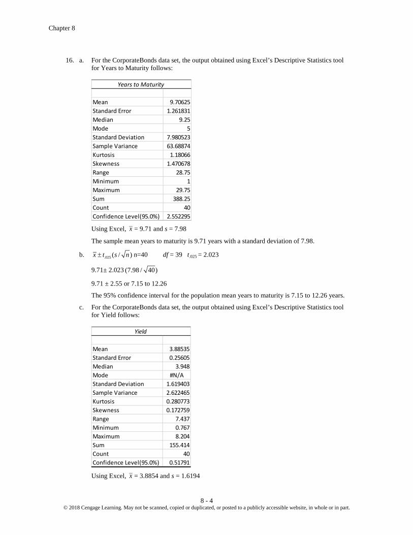
Chapter 8
8 - 4 © 2018 Cengage Learning. May not be scanned, copied or duplicated, or posted to a publicly accessible website, in whole or in part.
16. a. For the CorporateBonds data set, the output obtained using Excel’s Descriptive Statistics tool for Years to Maturity follows:
Using Excel, x = 9.71 and s = 7.98
The sample mean years to maturity is 9.71 years with a standard deviation of 7.98.
b. .025 ( / )x t s n± n=40 df = 39 t.025 = 2.023
9.71± 2.023 (7.98 / 40)
9.71 ± 2.55 or 7.15 to 12.26
The 95% confidence interval for the population mean years to maturity is 7.15 to 12.26 years.
c. For the CorporateBonds data set, the output obtained using Excel’s Descriptive Statistics tool for Yield follows:
Using Excel, x = 3.8854 and s = 1.6194
Years to Maturity
Mean 9.70625Standard Error 1.261831Median 9.25Mode 5Standard Deviation 7.980523Sample Variance 63.68874Kurtosis 1.18066Skewness 1.470678Range 28.75Minimum 1Maximum 29.75Sum 388.25Count 40Confidence Level(95.0%) 2.552295
Yield
Mean 3.88535Standard Error 0.25605Median 3.948Mode #N/AStandard Deviation 1.619403Sample Variance 2.622465Kurtosis 0.280773Skewness 0.172759Range 7.437Minimum 0.767Maximum 8.204Sum 155.414Count 40Confidence Level(95.0%) 0.51791

Interval Estimation
8 - 5 © 2018 Cengage Learning. May not be scanned, copied or duplicated, or posted to a publicly accessible website, in whole or in part.
The sample mean yield on corporate bonds is 3.8854% with a standard deviation of 1.6194. d. .025 ( / )x t s n± df = 39 t.025 = 2.023
3.8854 ± 2.023 (1.6194 / 40)
3.8854 ± .5180 or 3.3674 to 4.4033
The 95% confidence interval for the population mean yield is 3.3674 to 4.4033 percent. 18. For the JobSearch data set, the output obtained using Excel’s Descriptive Statistics tool follows:
Job Search Time (Weeks)
Mean 22 Standard Error 1.8794 Median 20 Mode 17 Standard Deviation 11.8862 Sample Variance 141.2821 Kurtosis 0.9030 Skewness 1.0062 Range 52 Minimum 0 Maximum 52 Sum 880 Count 40 Confidence Level(95.0%) 3.8014
a. x = 22 weeks b. margin of error = 3.8014 c. The 95% confidence interval is x ± margin of error / 2 ( / )x t s nα± with n=40 df = 39 t=2.023
22 ± 2.023 (11.8862 / 40) 22 ± 3.8014 or 18.20 to 25.80 d. The descriptive statistics output shows that the skewness is 1.0062. There is a moderate positive
skewness in this data set. This can be expected to exist in a population such as this. While the above results are acceptable, considering a slightly larger sample next time would be a good strategy.

Chapter 8
8 - 6 © 2018 Cengage Learning. May not be scanned, copied or duplicated, or posted to a publicly accessible website, in whole or in part.
20. a. For the AutoInsurance data set, the output obtained using Excel’s Descriptive Statistics toolfollows:
n=20 / 51,020 / 20 2551ix x n= Σ = =
The point estimate of the mean annual auto insurance premium in Michigan is $2551.
b. 2 2( ) ( 2551)
301.30771 20 1
i ix x xs
nΣ − Σ −
= = =− −
95% confidence interval: x ±t.025 ( / )s n df = 19
2551 ± 2.093 (301.3077 / 20)
$2551 ± 141.01 or $2409.99 to $2692.01 c. The 95% confidence interval for Michigan does not include the national average of $1503 for the
United States. We would be 95% confident that auto insurance premiums in Michigan are above the national average.
22. a. The Excel output from using the Descriptive Statistics analysis tool with the Guardians file is shown:
Revenue ($)
Mean 23100 Standard Error 726.991162 Median 22950 Mode #N/A Standard Deviation 3981.89458 Sample Variance 15855484.5 Kurtosis 1.87574748 Skewness 0.47956961 Range 20200 Minimum 13700 Maximum 33900 Sum 693000 Count 30
Annual Premium
Mean 2551Standard Error 67.37444Median 2545Mode 2545Standard Deviation 301.3077Sample Variance 90786.32Kurtosis 0.029671Skewness -0.14843Range 1207Minimum 1905Maximum 3112Sum 51020Count 20Confidence Level(95 0%) 141 0163

Interval Estimation
8 - 7 © 2018 Cengage Learning. May not be scanned, copied or duplicated, or posted to a publicly accessible website, in whole or in part.
Confidence Level(95.0%) 1486.86387 / 2 ( / )x t s nα± with n=30 df = 29 s=3981.89 t=2.045
23100 ± 2.045 (3981.89 / 30) 23100 ± 14686.86
The sample mean is 23,100 and the margin of error (Confidence Level) is 1486.86. The 95% confidence interval for the population mean is $21,613.14 to $24,586.86. We are 95%
confident that the population mean two-day ticket sales revenue per theater is between $21,613.14 and $24,586.86.
b. Mean number of customers per theater = 23,100/8.11 = 2848.34 c. Total number of customers = 4080(2848.34) = 11,621,227 (or 11,621,208 if calculated from the unrounded prior calculations) ≈ $11.6 million customers Total box office ticket sales for the three-day weekend = 4080(23,100) = $94,248,000 ≈ $94 million 24. a. Planning value of σ = Range/4 = 36/4 = 9
b. n zE
n= = = =. ( . ) ( ) .0252 2
2
2 2
2
196 93
34 57 35σ
Use
c. n n= = =( . ) ( ) .196 9
277 79 78
2 2
2 Use
25. a. 2 2
2
(1.96) (6.84) 79.88 Use 80(1.5)
n n= = =
b. 2 2
2
(1.645) (6.84) 31.65 Use 322
n n= = =
26. a. 2 2 2 2.025
2 2
(1.96) (.25) 24.01(.10)
zn
Eσ
= = = Use 25
If the normality assumption for the population appears questionable, this should be adjusted upward
to at least 30.
b. 2 2
2
(1.96) (.25) 49(.07)
n = = Use 49 to guarantee a margin of error no greater than .07. However, the US
EIA may choose to increase the sample size to a round number of 50
c. 2 2
2
(1.96) (.25) 96.04(.05)
n = = Use 97
For reporting purposes, the US EIA might decide to round up to a sample size of 100.
Chapter 8
8 - 8 © 2018 Cengage Learning. May not be scanned, copied or duplicated, or posted to a publicly accessible website, in whole or in part.
28. a. 2 2 2 2
/22 2
(1.645) (25) 187.92 Use 188(3)
zn n
Eα σ
= = = =
b. 2 2
2
(1.96) (25) 266.78 Use 267(3)
n n= = =
c. 2 2
2
(2.576) (25) 460.82 Use 461(3)
n n= = =
d. The sample size gets larger as the confidence level is increased. We would not recommend 99%
confidence. The sample size must be increased by 79 respondents (267 – 188) to go from 90% to 95%. This may be reasonable. However, increasing the sample size by 194 respondents (461 – 267) to go from 95% to 99% would probably be viewed as too expensive and time consuming for the 4% gain in confidence level.
30. 1.5σ =
2 2 2 2.025
2 2
(1.96) (1.5) 34.57 (.5)
znE
σ= = =
Use n = 35 to guarantee the margin of error will not exceed .5. 31. a. p = 100/400 = .25
b. (1 ) .25(.75) .0217400
p pn−
= =
c. p z p pn
±−
.( )
0251
.25 ± 1.96 (.0217) .25 ± .0424 or .2076 to .2924
32. a. .70 ± 1.645 .70(.30)800
.70 ± .0267 or .6733 to .7267
b. .70 ± 1.96 .70(.30)800
.70 ± .0318 or .6682 to .7318 34. Use planning value p = .50
2
2
(1.96) (.50)(.50) 1067.11 Use 1068(.03)
n n= = =

Interval Estimation
8 - 9 © 2018 Cengage Learning. May not be scanned, copied or duplicated, or posted to a publicly accessible website, in whole or in part.
35. a. p = 20901/45535 = .459 b. Margin of Error:
/ 2
(1 ) 0.459(0.541)1.645 .0038
45535
p pZ
nα
−= =
c. Confidence interval: .459± .0038 or .4552 to .4628 (.4552 to .4629 without any intermediary rounding) d. Margin of Error
/ 2
(1 ) 0.459(0.541)1.96 0.0046
45535
p pZ
nα
−= =
95% Confidence Interval .459± .0046 or .4544 to .4636 36. a. p = 46/200 = .23
b. .025(1 )p pp z
n−
±
.23 ± 1.96 (.23)(.77)200
.23 ± .0583 or .1717 to .2883 38. a. 29 /162 .1790p = = b. 104 /162p = = .6420
Margin of error = (1 ) (.642)(.358)1.96 1.96 .0738162
p pn−
= =
Confidence interval: .6420 ± .0738 or .5682 to .7158
c. 2
2
1.96 (.642)(.358) 353.18(.05)
n = = Use n = 354
39. a. 2 2.025
2 2
*(1 *) (1.96) (.17)(1 .17) 602.28(.03)
z p pnE
− −= = = Use n = 603
b. 2 2.005
2 2
*(1 *) (2.576) (.17)(1 .17) 1040.34(.03)
z p pn
E− −
= = = Use n = 1041
Chapter 8
8 - 10 © 2018 Cengage Learning. May not be scanned, copied or duplicated, or posted to a publicly accessible website, in whole or in part.
40. Margin of error: .025(1 ) .52(1 .52)1.96 .0346
800p pz
n− −
= =
95% Confidence interval: p ± .0346 .52 ± .0346 or .4854 to .5546
42. a. *(1 *) .50(1 .50) .0226491
p pn− −
= =
.025*(1 *)p pz
n− = 1.96(.0226) = .0442
b. 2.025
2
*(1 *)z p pn
E−
=
September 2
2
1.96 (.50)(1 .50) 600.25.04
n −= = Use 601
October 2
2
1.96 (.50)(1 .50) 1067.11.03
n −= = Use 1068
November 2
2
1.96 (.50)(1 .50) 2401.02
n −= =
Pre-Election 2
2
1.96 (.50)(1 .50) 9604.01
n −= =
44. Using Excel and the webfile FedTaxErrors, the sample mean is 326.6674x = and the sample size is n = 10001. The populationstandard deviation 12300σ = is known. a. ��𝑥 = 326.6674 b. 𝑧𝑧𝛼𝛼 2⁄ 𝜎𝜎𝑥𝑥 = 1.96(122.9939) = 241.0680 Using Excel for the margin of error: CONFIDENCE.NORM(.05,12300,10001) = 241.0635 c. ��𝑥 ± 𝑧𝑧𝛼𝛼 2⁄ 𝜎𝜎𝑥𝑥 = 326.6674 ± 241.0680 = (85.5994, 567.7354) or 85.6 to 567.7
46. a. ��𝑝 = 65120/102519 = .6352 (1 ) .6352(1 .6352) .0015102519p
p pn
σ − −= = =
b. 𝑧𝑧𝛼𝛼 2⁄ 𝜎𝜎𝑝𝑝 = 1.96(.0015) = .0029 c. ��𝑝 ± 𝑧𝑧𝛼𝛼 2⁄ 𝜎𝜎𝑝𝑝 = .6352 ± .0029 = (.6323, .6381)
48. a. Margin of error: .025151.96 4.0054
zn
σ= =
Using Excel for the margin of error: CONFIDENCE.NORM(.05,15,54) = 4.0 b. Confidence interval: x ± margin of error

Interval Estimation
8 - 11 © 2018 Cengage Learning. May not be scanned, copied or duplicated, or posted to a publicly accessible website, in whole or in part.
33.77 ± 4.00or $29.77 to $37.77 50. x =1873 n=80 a. Margin of error = t.025 ( / )s n df = 79t.025 = 1.990s = 550 1.990 (550 / 80) = 122 b. x ± margin of error 1873 ± 122 or $1751 to $1995 c. 92 million Americans are of age 50 and over Estimate of total expenditures = 92(1873) = 172,316 In dollars, we estimate that $172,316 million dollars are spent annually by Americans of age 50 and
over on restaurants and carryout food. d. We would expect the median to be less than the mean. The few individuals that spend much more
than the average cause the mean to be larger than the median. This is typical for data of this type. 52. a. For the DrugCost data set, the output obtained using Excel’s Descriptive Statistics tool for Total Annual Cost follows:
773x = and 738.3835s = n=400 df=399 t=1.6487 This can be obtained from Excel using: T.INV(.05,399)=1.6487
Margin of error = .05738.38351.6487 60.87
400stn
= =
Total Annual Cost
Mean 773Standard Error 36.91917Median 647Mode 0Standard Deviation 738.3835Sample Variance 545210.1Kurtosis -0.65717Skewness 0.577692Range 3366Minimum 0Maximum 3366Sum 309200Count 400Confidence Level(90.0%) 60.86796

Chapter 8
8 - 12 © 2018 Cengage Learning. May not be scanned, copied or duplicated, or posted to a publicly accessible website, in whole or in part.
90% Confidence Interval: 773 ± 60.87 or $712.13 to $833.87 b. For the DrugCost data set, the output obtained using Excel’s Descriptive Statistics tool for Employee Out-of-Pocket Cost follows:
187x = and 178.6207s = n=400 df =399 t= 1.6487 obtained from T.INV(.05,399)
Margin of error = .05178.62071.6487 14.72
400stn
= =
90% Confidence Interval: 187 ± 14.72 or $172.28 to $201.72 c. There were 136 employees who had no prescription medication cost for the year. 136 / 400 .34p = = d. The margin of error in part (a) is 60.87; the margin of error in part (c) is 14.72. The margin of error
in part (a) is larger because the sample standard deviation in part (a) is larger. The sample size and confidence level are the same in both parts.
54. n n= = =( . ) ( . ) .2 33 2 6
136 7 37
2 2
2 Use
56. n n= = =( . ) ( ) .196 675
10017503 176
2 2
2 Use
58. a. p = 200/369 = .5420
b. (1 ) (.5420)(.4580)1.96 1.96 .0508369
p pn−
= =
c. .5420 ± .0508 or .4912 to .5928
Employee Out-of-Pocket Cost
Mean 187Standard Error 8.931036Median 156.5Mode 0Standard Deviation 178.6207Sample Variance 31905.36Kurtosis -0.65777Skewness 0.57748Range 814Minimum 0Maximum 814Sum 74800Count 400Confidence Level(90.0%) 14.72443

Interval Estimation
8 - 13 © 2018 Cengage Learning. May not be scanned, copied or duplicated, or posted to a publicly accessible website, in whole or in part.
60. a. With 165 out of 750 respondents rating the economy as good or excellent, p = 165/750 = .22
b. Margin of error (1 ) .22(1 .22)1.96 1.96 .0296750
p pn− −
= = =
95% Confidence interval: .22 ± .0296 or .1904 to .2496 c. With 315 out of 750 respondents rating the economy as poor, p = 315/750 = .42
Margin of error (1 ) .42(1 .42)1.96 1.96 .0353750
p pn− −
= = =
95% Confidence interval: .42 ± .0353 or .3847 to .4553 d. The confidence interval in part (c) is wider. This is because the sample proportion is closer to .5 in
part (c).
62. a. 2
2
(2.33) (.70)(.30) 1266.74 Use 1267(.03)
n n= = =
b. 2
2
(2.33) (.50)(.50) 1508.03 Use 1509(.03)
n n= = =
64. a. n = 1993 p = 618/1993 = .3101
b. p p p±
−196 11993
. ( )
.3101 ± 1.96 (.3101)(.6899)1993
.3101 ± .0203 or .2898 to .3304
c. 2
2
*(1 *)z p pnE
−=
2
2
(1.96) (.3101)(.6899) 8218.64 Use 8219(.01)
z n= = =
No; the sample appears unnecessarily large. The .02 margin of error reported in part (b) should
provide adequate precision.

9 - 1 © 2018 Cengage Learning. May not be scanned, copied or duplicated, or posted to a publicly accessible website, in whole or in part.
Chapter 9 Hypothesis Tests Solutions:
2. a. H0: µ≤ 14 Ha: µ> 14 Research hypothesis b. There is no statistical evidence that the new bonus plan increases sales volume. c. The research hypothesis that µ> 14 is supported. We can conclude that the new bonus plan
increases the mean sales volume. 4. a. H0: µ≥ 220 Ha: µ< 220 Research hypothesis to see if mean cost is less than $220. b. We are unable to conclude that the new method reduces costs. c. Conclude µ< 220. Consider implementing the new method based on the conclusion that it lowers
the mean cost per hour. 5. a. Conclude that the population mean monthly cost of electricity in the Chicago neighborhood is
greater than $104 and hence higher than in the comparable neighborhood in Cincinnati. b. The Type I error is rejecting H0 when it is true. This error occurs if the researcher concludes that the
population mean monthly cost of electricity is greater than $104 in the Chicago neighborhood when the population mean cost is actually less than or equal to $104.
c. The Type II error is accepting H0 when it is false. This error occurs if the researcher concludes that
the population mean monthly cost for the Chicago neighborhood is less than or equal to $104 when it is not.
6. a. H0: µ≤ 1 The label claim or assumption. Ha: µ> 1 b. Claiming µ> 1 when it is not. This is the error of rejecting the product’s claim when the claim is
true. c. Concluding µ≤ 1 when it is not. In this case, we miss the fact that the product is not meeting its
label specification.
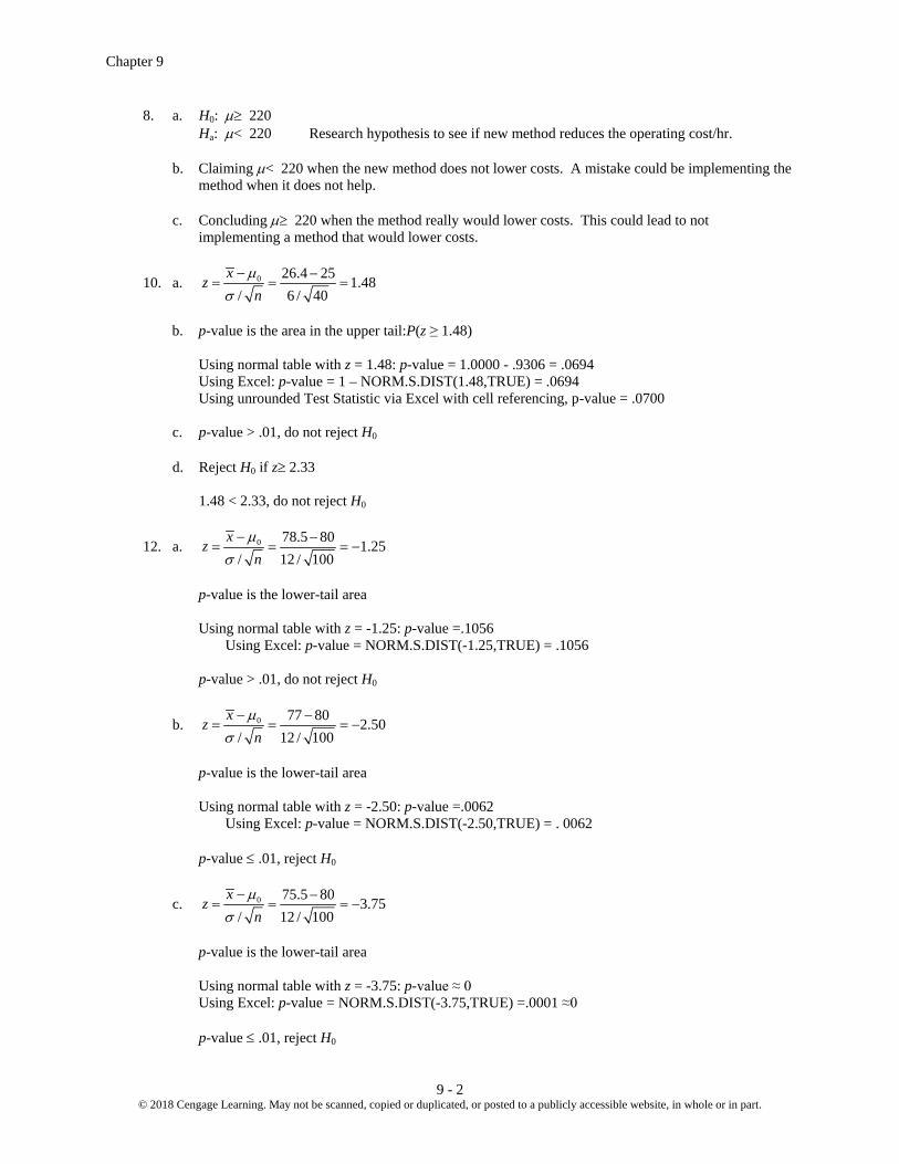
Chapter 9
9 - 2 © 2018 Cengage Learning. May not be scanned, copied or duplicated, or posted to a publicly accessible website, in whole or in part.
8. a. H0: µ≥ 220 Ha: µ< 220 Research hypothesis to see if new method reduces the operating cost/hr. b. Claiming µ< 220 when the new method does not lower costs. A mistake could be implementing the
method when it does not help. c. Concluding µ≥ 220 when the method really would lower costs. This could lead to not
implementing a method that would lower costs.
10. a. 0 26.4 25 1.48/ 6 / 40
xzn
µσ
− −= = =
b. p-value is the area in the upper tail:P(z ≥ 1.48) Using normal table with z = 1.48: p-value = 1.0000 - .9306 = .0694 Using Excel: p-value = 1 – NORM.S.DIST(1.48,TRUE) = .0694 Using unrounded Test Statistic via Excel with cell referencing, p-value = .0700 c. p-value > .01, do not reject H0 d. Reject H0 if z≥ 2.33 1.48 < 2.33, do not reject H0
12. a. 0 78.5 80 1.25/ 12 / 100
xzn
µσ
− −= = = −
p-value is the lower-tail area Using normal table with z = -1.25: p-value =.1056 Using Excel: p-value = NORM.S.DIST(-1.25,TRUE) = .1056 p-value > .01, do not reject H0
b. 0 77 80 2.50/ 12 / 100
xzn
µσ
− −= = = −
p-value is the lower-tail area Using normal table with z = -2.50: p-value =.0062 Using Excel: p-value = NORM.S.DIST(-2.50,TRUE) = . 0062 p-value ≤ .01, reject H0
c. 0 75.5 80 3.75/ 12 / 100
xzn
µσ
− −= = = −
p-value is the lower-tail area Using normal table with z = -3.75: p-value ≈ 0 Using Excel: p-value = NORM.S.DIST(-3.75,TRUE) =.0001 ≈0 p-value ≤ .01, reject H0
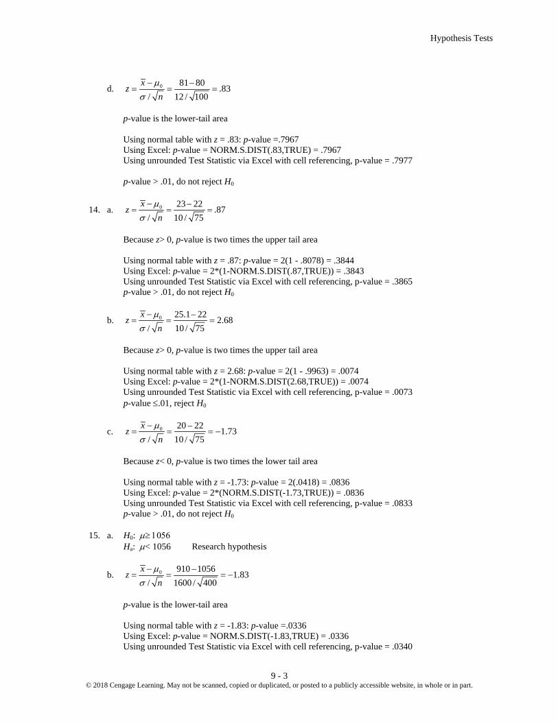
Hypothesis Tests
9 - 3 © 2018 Cengage Learning. May not be scanned, copied or duplicated, or posted to a publicly accessible website, in whole or in part.
d. 0 81 80 .83/ 12 / 100
xzn
µσ
− −= = =
p-value is the lower-tail area Using normal table with z = .83: p-value =.7967 Using Excel: p-value = NORM.S.DIST(.83,TRUE) = .7967 Using unrounded Test Statistic via Excel with cell referencing, p-value = .7977 p-value > .01, do not reject H0
14. a. 0 23 22 .87/ 10 / 75
xzn
µσ
− −= = =
Because z> 0, p-value is two times the upper tail area Using normal table with z = .87: p-value = 2(1 - .8078) = .3844 Using Excel: p-value = 2*(1-NORM.S.DIST(.87,TRUE)) = .3843 Using unrounded Test Statistic via Excel with cell referencing, p-value = .3865 p-value > .01, do not reject H0
b. 0 25.1 22 2.68/ 10 / 75
xzn
µσ
− −= = =
Because z> 0, p-value is two times the upper tail area Using normal table with z = 2.68: p-value = 2(1 - .9963) = .0074 Using Excel: p-value = 2*(1-NORM.S.DIST(2.68,TRUE)) = .0074 Using unrounded Test Statistic via Excel with cell referencing, p-value = .0073 p-value ≤.01, reject H0
c. 0 20 22 1.73/ 10 / 75
xzn
µσ
− −= = = −
Because z< 0, p-value is two times the lower tail area Using normal table with z = -1.73: p-value = 2(.0418) = .0836 Using Excel: p-value = 2*(NORM.S.DIST(-1.73,TRUE)) = .0836 Using unrounded Test Statistic via Excel with cell referencing, p-value = .0833 p-value > .01, do not reject H0 15. a. H0: µ≥ 1056 Ha: µ< 1056 Research hypothesis
b. 0 910 1056 1.83/ 1600 / 400
xzn
µσ
− −= = = −
p-value is the lower-tail area Using normal table with z = -1.83: p-value =.0336 Using Excel: p-value = NORM.S.DIST(-1.83,TRUE) = .0336 Using unrounded Test Statistic via Excel with cell referencing, p-value = .0340

Chapter 9
9 - 4 © 2018 Cengage Learning. May not be scanned, copied or duplicated, or posted to a publicly accessible website, in whole or in part.
c. p-value ≤ .05, reject H0. Conclude the mean refund of “last minute” filers is less than $1056. d. Reject H0 if z≤-1.645 -1.83 ≤ -1.645, reject H0 16. a. H0: µ≤ 3173 Ha: µ> 3173 Research hypothesis
b. 0 3325 3173 2.04/ 1000 / 180
xz
nµ
σ− −
= = =
p-value is the upper tail area or P(z ≥ 2.04) Using normal table withz = 2.04:p-value = 1.0000 - .9793 = .0207 Using Excel: p-value = 1-NORM.S.DIST(2.04,TRUE) = .0207 Using unrounded Test Statistic via Excel with cell referencing, p-value = .0207 c. p-value< .05. Reject H0. The current population mean credit card balance for undergraduate
students has increased compared to the previous all-time high of $3173 reported in April 2009. 18. a. H0: µ= 192 Ha: µ≠ 192 Research hypothesis
b. 0 182 192 2.23/ 55 / 150
xz
nµ
σ− −
= = = −
Because z< 0, p-value is two times the lower tail area Using normal table with z = – 2.23: p-value = 2(.0129) = .0258 Using Excel: p-value = 2*NORM.S.DIST(-2.23,TRUE)= .0257 Using unrounded Test Statistic via Excel with cell referencing, p-value = .0260 c. p-value = .0258 .05α≤ =
Reject H0 and conclude that the mean number of restaurant meals eaten by young millennials has changed in 2012.
20. a. H0: µ≥ 838 Ha: µ< 838 Research hypothesis
b. 0 745 838 2.40/ 300 60
xz
nµ
σ− −
= = = −
c. Lower tail p-value is area to left of the test statistic. Using normal table with z = -2.40: p-value = .0082. Using Excel: p-value = NORM.S.DIST(-2.40,TRUE)= .0082 Using unrounded Test Statistic via Excel with cell referencing, p-value = .0082 d. p-value ≤ .01; reject 0H . Conclude that the annual expenditure per person on prescription drugs is less in the Midwest than in the Northeast.

Hypothesis Tests
9 - 5 © 2018 Cengage Learning. May not be scanned, copied or duplicated, or posted to a publicly accessible website, in whole or in part.
22. a. H0: µ= 8 Ha: µ≠ 8 Research hypothesis
b. 8.4 8.0 1.37/ 3.2 / 120
xzn
µσ
− −= = =
Because z> 0, p-value is two times the upper tail area Using normal table with z = 1.37: p-value = 2(1 - .9147) = .1706 Using Excel: p-value = 2*(1-NORM.S.DIST(1.37,TRUE)) = .1707 Using unrounded Test Statistic via Excel with cell referencing, p-value = .1709 c. p-value > .05, do not reject H0. Cannot conclude that the population mean waiting time differs from
8 minutes. d. .025 ( / )x z nσ± 8.4 ± 1.96 (3.2 / 120) 8.4 ± .57 (7.83 to 8.97) Yes; µ= 8 is in the interval. Do not reject H0.
24. a. 0 17 18 1.54/ 4.5 / 48
xts n
µ− −= = = −
b. Degrees of freedom = n – 1 = 47
Because t< 0, p-value is two times the lower tail area Using t table: area in lower tail is between .05 and .10; therefore, p-value isbetween .10 and .20. Using Excel: p-value = 2*T.DIST(-1.54,47,TRUE) = .1303 Using unrounded Test Statistic via Excel with cell referencing, p-value = .1304 c. p-value > .05, do not reject H0. d. With df = 47, t.025 = 2.012 Reject H0 if t≤ -2.012 or t≥2.012 t = -1.54; do not reject H0
26. a. 0 103 100 2.10/ 11.5 / 65
xts n
µ− −= = =
Degrees of freedom = n – 1 = 64 Because t> 0, p-value is two times the upper tail area
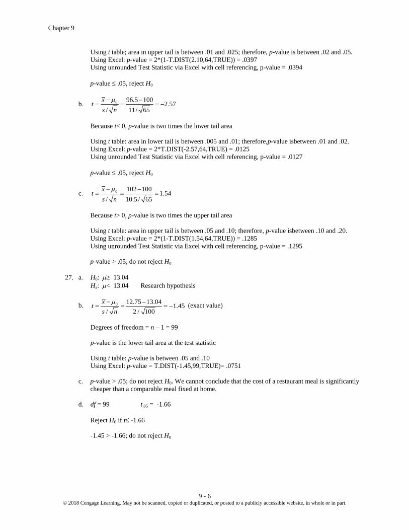
Chapter 9
9 - 6 © 2018 Cengage Learning. May not be scanned, copied or duplicated, or posted to a publicly accessible website, in whole or in part.
Using t table; area in upper tail is between .01 and .025; therefore, p-value is between .02 and .05. Using Excel: p-value = 2*(1-T.DIST(2.10,64,TRUE)) = .0397 Using unrounded Test Statistic via Excel with cell referencing, p-value = .0394 p-value ≤ .05, reject H0
b. 0 96.5 100 2.57/ 11/ 65
xts n
µ− −= = = −
Because t< 0, p-value is two times the lower tail area Using t table: area in lower tail is between .005 and .01; therefore,p-value isbetween .01 and .02. Using Excel: p-value = 2*T.DIST(-2.57,64,TRUE) = .0125 Using unrounded Test Statistic via Excel with cell referencing, p-value = .0127 p-value ≤ .05, reject H0
c. 0 102 100 1.54/ 10.5 / 65
xts n
µ− −= = =
Because t> 0, p-value is two times the upper tail area Using t table: area in upper tail is between .05 and .10; therefore, p-value isbetween .10 and .20. Using Excel: p-value = 2*(1-T.DIST(1.54,64,TRUE)) = .1285 Using unrounded Test Statistic via Excel with cell referencing, p-value = .1295 p-value > .05, do not reject H0 27. a. H0: µ≥ 13.04 Ha: µ< 13.04 Research hypothesis
b. 0 12.75 13.04 1.45/ 2 / 100
xt
s nµ− −
= = = − (exact value)
Degrees of freedom = n – 1 = 99 p-value is the lower tail area at the test statistic Using t table: p-value is between .05 and .10 Using Excel: p-value = T.DIST(-1.45,99,TRUE)= .0751 c. p-value > .05; do not reject H0. We cannot conclude that the cost of a restaurant meal is significantly
cheaper than a comparable meal fixed at home. d. df = 99 t.05 = -1.66 Reject H0 if t≤ -1.66 -1.45 > -1.66; do not reject H0
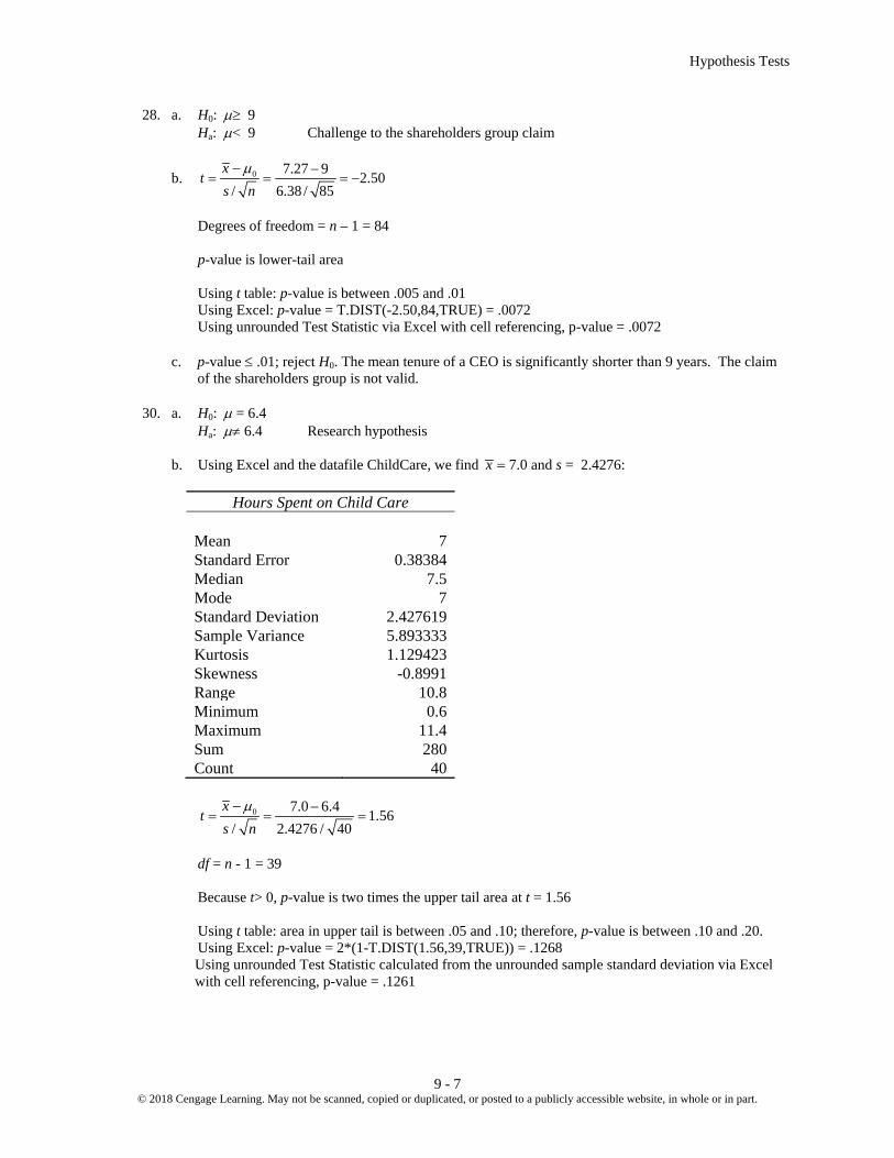
Hypothesis Tests
9 - 7 © 2018 Cengage Learning. May not be scanned, copied or duplicated, or posted to a publicly accessible website, in whole or in part.
28. a. H0: µ≥ 9 Ha: µ< 9 Challenge to the shareholders group claim
b. 0 7.27 9 2.50/ 6.38 / 85
xt
s nµ− −
= = = −
Degrees of freedom = n – 1 = 84 p-value is lower-tail area Using t table: p-value is between .005 and .01 Using Excel: p-value = T.DIST(-2.50,84,TRUE) = .0072 Using unrounded Test Statistic via Excel with cell referencing, p-value = .0072 c. p-value ≤ .01; reject H0. The mean tenure of a CEO is significantly shorter than 9 years. The claim
of the shareholders group is not valid. 30. a. H0: µ = 6.4 Ha: µ≠ 6.4 Research hypothesis b. Using Excel and the datafile ChildCare, we find 7.0x = and s = 2.4276:
Hours Spent on Child Care
Mean 7 Standard Error 0.38384 Median 7.5 Mode 7 Standard Deviation 2.427619 Sample Variance 5.893333 Kurtosis 1.129423 Skewness -0.8991 Range 10.8 Minimum 0.6 Maximum 11.4 Sum 280 Count 40
0 7.0 6.4 1.56/ 2.4276 / 40
xt
s nµ− −
= = =
df = n - 1 = 39 Because t> 0, p-value is two times the upper tail area at t = 1.56 Using t table: area in upper tail is between .05 and .10; therefore, p-value is between .10 and .20. Using Excel: p-value = 2*(1-T.DIST(1.56,39,TRUE)) = .1268 Using unrounded Test Statistic calculated from the unrounded sample standard deviation via Excel
with cell referencing, p-value = .1261
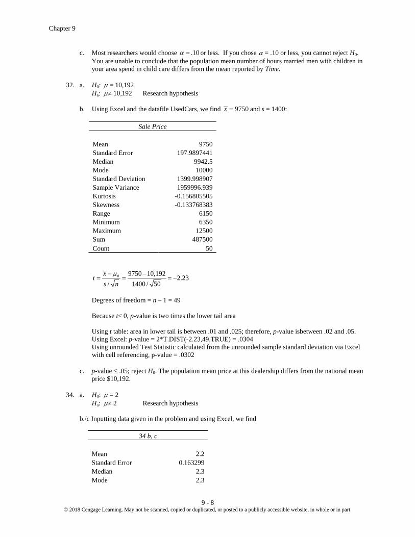
Chapter 9
9 - 8 © 2018 Cengage Learning. May not be scanned, copied or duplicated, or posted to a publicly accessible website, in whole or in part.
c. Most researchers would choose .10α = or less. If you chose α = .10 or less, you cannot reject H0. You are unable to conclude that the population mean number of hours married men with children in your area spend in child care differs from the mean reported by Time.
32. a. H0: µ = 10,192 Ha: µ≠ 10,192 Research hypothesis b. Using Excel and the datafile UsedCars, we find 9750x = and s = 1400:
Sale Price
Mean 9750 Standard Error 197.9897441 Median 9942.5 Mode 10000 Standard Deviation 1399.998907 Sample Variance 1959996.939 Kurtosis -0.156805505 Skewness -0.133768383 Range 6150 Minimum 6350 Maximum 12500 Sum 487500 Count 50
0 9750 10,192 2.23/ 1400 / 50
xts n
µ− −= = = −
Degrees of freedom = n – 1 = 49 Because t< 0, p-value is two times the lower tail area Using t table: area in lower tail is between .01 and .025; therefore, p-value isbetween .02 and .05. Using Excel: p-value = 2*T.DIST(-2.23,49,TRUE) = .0304 Using unrounded Test Statistic calculated from the unrounded sample standard deviation via Excel
with cell referencing, p-value = .0302 c. p-value ≤ .05; reject H0. The population mean price at this dealership differs from the national mean
price $10,192. 34. a. H0: µ = 2 Ha: µ≠ 2 Research hypothesis b./c Inputting data given in the problem and using Excel, we find
34 b, c
Mean 2.2 Standard Error 0.163299 Median 2.3 Mode 2.3

Hypothesis Tests
9 - 9 © 2018 Cengage Learning. May not be scanned, copied or duplicated, or posted to a publicly accessible website, in whole or in part.
Standard Deviation 0.516398 Sample Variance 0.266667 Kurtosis -0.73359 Skewness -0.33283 Range 1.6 Minimum 1.4 Maximum 3 Sum 22 Count 10
Using formulas:
22 2.210
ixxn
Σ= = =
c. ( )2
.5161
ix xs
nΣ −
= =−
d. 0 2.2 2 1.22/ .516 / 10
xts n
µ− −= = =
Degrees of freedom = n - 1 = 9 Because t> 0, p-value is two times the upper tail area Using t table: area in upper tail is between .10 and .20; therefore, p-value is between .20 and .40. Using Excel: p-value = 2*(1-T.DIST(1.22,9,TRUE)) = .2535 Using unrounded Test Statistic calculated from the unrounded sample standard deviation via Excel
with cell referencing, p-value = .2518 e. p-value > .05; do not reject H0. No reason to change from the 2 hours for cost estimating purposes.
36. a. 0
0 0
.68 .75 2.80(1 ) .75(1 .75)
300
p pzp p
n
− −= = = −
− − (exact value)
p-value is lower-tail area Using normal table with z = -2.80: p-value =.0026 Using Excel: p-value = NORM.S.DIST(-2.80,TRUE) = .0026 p-value ≤ .05; reject H0. The proportion is less than .75.
b. .72 .75 1.20.75(1 .75)
300
z −= = −
− (exact value)
p-value is lower-tail area Using normal table with z = -1.20: p-value =.1151 Using Excel: p-value = NORM.S.DIST(-1.20,TRUE) = .1151 p-value > .05; do not reject H0. We cannot conclude that the proportion is less than .75.

Chapter 9
9 - 10 © 2018 Cengage Learning. May not be scanned, copied or duplicated, or posted to a publicly accessible website, in whole or in part.
c. .70 .75 2.00.75(1 .75)
300
z −= = −
− (exact value)
p-value is lower-tail area Using normal table with z = -2.00: p-value =.0228 Using Excel: p-value = NORM.S.DIST(-2.00,TRUE) = . 0228 p-value ≤ .05; reject H0. The proportion is less than .75.
d. .77 .75 .80.75(1 .75)
300
z −= =
− (exact value)
p-value is lower-tail area Using normal table with z = .80: p-value =.7881 Using Excel: p-value = NORM.S.DIST(.80,TRUE) = . 7881 p-value > .05; do not reject H0. We cannot conclude that the proportion is less than .75. 38. a. H0: p= .64 Ha: p≠ .64 Research hypothesis
b. 52 .52100
p = =
0
0 0
.52 .64 2.50(1 ) .64(1 .64)
100
p pzp p
n
− −= = = −
− − (exact value)
Because z< 0, p-value is two times the lower tail area Using normal table with z = -2.50: p-value = 2(.0062) = .0124 Using Excel: p-value = 2*NORM.S.DIST(-2.50,TRUE) = . 0124 c. p-value ≤ .05; reject H0. Proportion differs from the reported .64. d. Yes. Since p = .52, it indicates that fewer than 64% of the shoppers believe the supermarket brand is
as good as the name brand. 40. a. Sample proportion: .35p = Number planning to provide holiday gifts: 60(.35) 21np = = b. H0: p≥ .46 Ha: p< .46 Research hypothesis
0
0 0
.35 .46 1.71(1 ) .46(1 .46)
60
p pz
p pn
− −= = = −
− −
p-value is area in lower tail
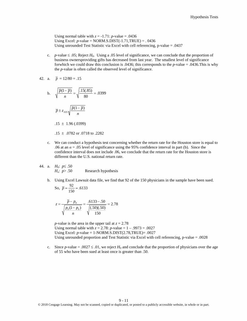
Hypothesis Tests
9 - 11 © 2018 Cengage Learning. May not be scanned, copied or duplicated, or posted to a publicly accessible website, in whole or in part.
Using normal table with z = -1.71: p-value = .0436 Using Excel: p-value = NORM.S.DIST(-1.71,TRUE) = . 0436 Using unrounded Test Statistic via Excel with cell referencing, p-value = .0437 c. p-value ≤ .05; Reject H0. Using a .05 level of significance, we can conclude that the proportion of
business ownersproviding gifts has decreased from last year. The smallest level of significance forwhich we could draw this conclusion is .0436; this corresponds to the p-value = .0436.This is why the p-value is often called the observed level of significance.
42. a. p = 12/80 = .15
b. (1 ) .15(.85) .0399
80p p
n−
= =
p z p pn
±−
.( )
0251
.15 ± 1.96 (.0399) .15 ± .0782 or .0718 to .2282 c. We can conduct a hypothesis test concerning whether the return rate for the Houston store is equal to
.06 at an α = .05 level of significance using the 95% confidence interval in part (b). Since the confidence interval does not include .06, we conclude that the return rate for the Houston store is different than the U.S. national return rate.
44. a. H0: p≤ .50 Ha: p> .50 Research hypothesis b. Using Excel Lawsuit data file, we find that 92 of the 150 physicians in the sample have been sued.
So, 92 .6133150
p = =
0
0 0
.6133 .50 2.78(1 ) (.50)(.50)
150
p pz
p pn
− −= = =
−
p-value is the area in the upper tail at z = 2.78 Using normal table with z = 2.78: p-value = 1 – .9973 = .0027 Using Excel: p-value = 1-NORM.S.DIST(2.78,TRUE)= .0027 Using unrounded proportion and Test Statistic via Excel with cell referencing, p-value = .0028 c. Since p-value = .0027 ≤ .01, we reject H0 and conclude that the proportion of physicians over the age
of 55 who have been sued at least once is greater than .50.

Chapter 9
9 - 12 © 2018 Cengage Learning. May not be scanned, copied or duplicated, or posted to a publicly accessible website, in whole or in part.
46. H0: µ= 101.5 Ha: µ≠ 101.5 Research hypothesis Using the FedEmail datafile and Excel, the sample mean, 100.47x =
100.47 101.50 4.1525 10163
xz
n
µ
σ
− −= = = −
Because z< 0, p-value is two times the lower tail area Using normal table with z = -4.15: p-value ≈ 2(.0000) = .0000 Using Excel: p-value = 2*(NORM.S.DIST(-4.15,TRUE)) = .0000 Using the unrounded sample mean to calculate the Test Statistic via Excel with cell referencing, p-
value = .0000
p-value ≤ .01, reject H0. Conclude that the actual mean number of business emails sent and received per business day by employees of thisdepartment of the Federal Government differs from corporate employees.
Although the difference between the sample mean number of business emails sent and received per
business day by employees of this department of the Federal Government and the mean number of business emails sent and received by corporate employees is statistically significant, this difference of 1.03 emails is relatively small and so may be of little or no practical significance.
48. H0: p≤.62 Ha: p>.62 Research hypothesis
31038 .62649581
p = = ( ) ( )0
0 0
.626 .62 2.751 .62 1 .62
49581
p pzp p
n
− −= = =
− −
p-value is the area in the upper tail Using normal table with z = 2.75: p-value = 1 - .9970 = .0030 Using Excel: p-value = 1-NORM.S.DIST(2.75,TRUE) = .0030 Using unrounded proportion and Test Statistic via Excel with cell referencing, p-value = .0029
p-value ≤ .05, reject H0. Conclude that the actual proportion of fast food orders this year that includes French fries exceeds the proportion of fast food orders that included French frieslast year.
Although the difference between the sample proportion of fast food orders this year that includes
French fries and the proportion of fast food orders that included French frieslast year is statistically significant, APGA should be concerned about whether this .006 or .6% increase is large enough to be effective in an advertising campaign.
50. a. H0: µ = 16 Ha: µ≠ 16 Research hypothesis to test for over or under filling
b. 0 16.32 16 2.19/ .8 / 30
xzn
µσ
− −= = =
Because z> 0, p-value is two times the upper tail area Using normal table with z = 2.19: p-value = 2(.0143) = .0286

Hypothesis Tests
9 - 13 © 2018 Cengage Learning. May not be scanned, copied or duplicated, or posted to a publicly accessible website, in whole or in part.
Using Excel: p-value = 2*(1-NORM.S.DIST(2.19,TRUE)) = . 0285 Using unrounded Test Statistic via Excel with cell referencing, p-value = .0285 p-value ≤ .05; reject H0. Readjust production line.
c. 0 15.82 16 1.23/ .8 / 30
xzn
µσ
− −= = = −
Because z< 0, p-value is two times the lower tail area Using normal table with z = -1.23: p-value = 2(.1093) = .2186 Using Excel: p-value = 2*NORM.S.DIST(-1.23,TRUE) = . 2187 Using unrounded Test Statistic via Excel with cell referencing, p-value = .2178 p-value > .05; do not reject H0. Continue the production line. d. Reject H0 if z≤ -1.96 or z≥ 1.96 For x = 16.32, z = 2.19; reject H0
For x = 15.82, z = -1.23; do not reject H0 Yes, same conclusion. 52. a. H0: µ≤ 4 Ha: µ> 4 Research hypothesis
b. 0 4.5 4 2.58/ 1.5 / 60
xz
nµ
σ− −
= = =
p-value is the upper tail area at z =2.58 Using normal table with z = 2.58: p-value = 1.0000 - .9951 = .0049 Using Excel: p-value = 1-NORM.S.DIST(2.58,TRUE) = . 0049 Using unrounded Test Statistic via Excel with cell referencing, p-value = .0049 c. p-value ≤ .01, reject H0. Conclude that the mean daily background television that children
from low-income families are exposed to is greater than four hours. 54. H0: µ≤ 30.8 Ha: µ> 30.8 Research hypothesis Using Excel and the datafile BritainMarriages, we find 32.72x = and s = 12.10:
Age
Mean 32.72340426 Standard Error 1.76556174 Median 31 Mode 21 Standard Deviation 12.10408147 Sample Variance 146.5087882 Kurtosis 2.118162618

Chapter 9
9 - 14 © 2018 Cengage Learning. May not be scanned, copied or duplicated, or posted to a publicly accessible website, in whole or in part.
Skewness 1.282462905 Range 56 Minimum 18 Maximum 74 Sum 1538 Count 47
��𝑥= 32.72 s = 12.10 𝑡𝑡 = 𝑥𝑥−𝜇𝜇0
𝑠𝑠 √𝑛𝑛⁄= 32.72−30.8
12.10 √47⁄= 1.09
Degrees of freedom = 47 - 1 = 46 p-value is the upper tail area Using t table: area in upper tail is between .10 and .20; therefore, p-value is between .10 and .20. Using Excel: p-value = 1 - T.DIST(1.09,46,TRUE) = 0.1407 Using unrounded Test Statistic calculated from the unrounded sample standard deviation via Excel
with cell referencing, p-value = .1408 p-value > .05; do not reject H0. The mean age of British men at the time of marriage exceeds the 2013 mean age of 30.8. 56. H0: µ≤ 125,000 Chamber of Commerce claim Ha: µ> 125,000
0 130,000 125,000 2.26/ 12,500 / 32
xts n
µ− −= = =
Degrees of freedom = 32 – 1 = 31 p-value is upper-tail area Using t table: p-value is between .01 and .025 Using Excel: p-value = 1-T.DIST(2.26,31,TRUE) = .0155 Using unrounded Test Statistic via Excel with cell referencing, p-value = .0154
p-value ≤ .05; reject H0. Conclude that the mean cost is greater than $125,000 per lot. 58. a. H0: p≤ .52 Ha: p> .52 Research hypothesis
285 .5588510
p = =
0
0 0
.5588 .52 1.75(1 ) .52(1 .52)
510
p pz
p pn
− −= = =
− −
p-value is the area in the upper tail Using normal table with z = 1.75: p-value = 1.0000 - .9599 = .0401

Hypothesis Tests
9 - 15 © 2018 Cengage Learning. May not be scanned, copied or duplicated, or posted to a publicly accessible website, in whole or in part.
Using Excel: p-value = 1-NORM.S.DIST(1.75,TRUE) = .0401 Using unrounded proportion and Test Statistic via Excel with cell referencing, p-value = .0396 p-value ≤ .05; reject H0. We conclude that people who fly frequently are more likely to be able to
sleep during flights. b. H0: p≤ .52 Ha: p> .52
285 .5588510
p = =
0
0 0
.5588 .52 1.75(1 ) .52(1 .52)
510
p pz
p pn
− −= = =
− −
p-value is the area in the upper tail Using normal table with z = 1.75: p-value = 1.0000 - .9599 = .0401 Using Excel: p-value = 1-NORM.S.DIST(1.75,TRUE) = .0401 Using unrounded proportion and Test Statistic via Excel with cell referencing, p-value = .0396 p-value > .01; we cannot reject H0. Thus, we cannot conclude that that people who fly frequently
better more likely to be able to sleep during flights. 60. a. H0: p≤ .30 Organization claim Ha: p> .30 Research hypothesis
b. 136 .34400
p = = (34%)
c. 0
0 0
.34 .30 1.75(1 ) .30(1 .30)
400
p pz
p pn
− −= = =
− −
p-value is the upper-tail area Using normal table with z = 1.75: p-value = 1.0000 - .9599 = .0401 Using Excel: p-value = 1-NORM.S.DIST(1.75,TRUE) = .0401 Using unrounded Test Statistic via Excel with cell referencing, p-value = .0404
d. p-value ≤ .05; reject H0. Conclude that more than 30% of the millennials either live at home with their parents or are otherwise dependent on their parents.
62. H0: p≥ .90 Radio station claim Ha: p< .90 Research hypothesis
49 .844858
p = =
0
0 0
.8448 .90 1.40(1 ) .90(1 .90)
58
p pzp p
n
− −= = = −
− −
p-value is the lower-tail area

Chapter 9
9 - 16 © 2018 Cengage Learning. May not be scanned, copied or duplicated, or posted to a publicly accessible website, in whole or in part.
Using normal table with z = -1.40: p-value =.0808 Using Excel: p-value = NORM.S.DIST(-1.40,TRUE) = . 0808 Using unrounded proportion and Test Statistic via Excel with cell referencing, p-value = .0807 p-value > .05; do not reject H0. Claim of at least 90% cannot be rejected.
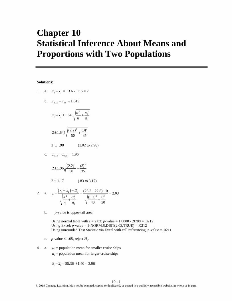
10 - 1 © 2018 Cengage Learning. May not be scanned, copied or duplicated, or posted to a publicly accessible website, in whole or in part.
Chapter 10 Statistical Inference About Means and Proportions with Two Populations Solutions: 1. a. x x1 2− = 13.6 - 11.6 = 2 b. / 2 .05z zα = = 1.645
2 21 2
1 21 2
1.645x xn nσ σ
− ± +
2 2(2.2) (3)2 1.645
50 35± +
2 ± .98 (1.02 to 2.98) c. / 2 .025z zα = = 1.96
2 2(2.2) (3)2 1.96
50 35± +
2 ± 1.17 (.83 to 3.17)
2. a. ( )1 2 0
2 2 2 21 2
1 2
(25.2 22.8) 0 2.03(5.2) 6
40 50
x x Dz
n nσ σ
− − − −= = =
++
b. p-value is upper-tail area
Using normal table with z = 2.03: p-value = 1.0000 - .9788 = .0212 Using Excel: p-value = 1-NORM.S.DIST(2.03,TRUE) = .0212 Using unrounded Test Statistic via Excel with cell referencing, p-value = .0211 c. p-value ≤ .05, reject H0. 4. a. 1µ = population mean for smaller cruise ships 2µ = population mean for larger cruise ships 1 2x x− = 85.36–81.40 = 3.96

Chapter 10
10 - 2 © 2018 Cengage Learning. May not be scanned, copied or duplicated, or posted to a publicly accessible website, in whole or in part.
b. 2 21 2
.0251 2
zn nσ σ
+
2 2(4.55) (3.97)1.96 1.88
37 44+ =
c. 3.96±1.88 (2.08 to 5.84) 6. 1µ = mean hotel price in Atlanta 2µ = mean hotel price in Houston H0: 1 2 0µ µ− ≥ Ha: 1 2 0µ µ− < Research hypothesis Using the Hotel data file and Excel’s Data Analysis Tool, the Two Sample z-Test results are:
z-Test: Two Sample for Means Atlanta Houston
Mean 91.71429 101.125 Known Variance 400 625 Observations 35 40 Hypothesized Mean Difference 0
z -1.8093 P(Z<=z) one-tail 0.035202 z Critical one-tail 1.644854 P(Z<=z) two-tail 0.070405 z Critical two-tail 1.959964
( )1 2 0
2 2 2 21 2
1 2
(91.71 101.13) 0 1.8120 2535 40
x x Dz
n nσ σ
− − − −= = = −
++
p-value is the lower-tail area
Using normal table with z = -1.81: p-value =.0351 Using Excel: p-value = NORM.S.DIST(-1.81,TRUE) = .0351 Using unrounded Test Statistic via Excel with cell referencing, p-value = .0352 p-value ≤ .05; reject H0. The mean price of a hotel room in Atlanta is lower than the mean price of a
hotel room in Houston. 8. a. 1µ = population mean Year 2 score 2µ = population mean Year 1 score H0: 1 2 0µ µ− ≤
Ha: 1 2 0µ µ− > Research hypothesis

Statistical Inference About Means and Proportions with Two Populations
10 - 3 © 2018 Cengage Learning. May not be scanned, copied or duplicated, or posted to a publicly accessible website, in whole or in part.
( )1 2
2 2 2 21 2
1 2
(76 73) 2.746 660 60
x xz
n nσ σ
− −= = =
++
p-value is upper-tail area
Using normal table with z = 2.74: p-value = 1.0000 - .9969 = .0031 Using Excel: p-value = 1-NORM.S.DIST(2.74,TRUE) = .0031 Using unrounded Test Statistic via Excel with cell referencing, p-value = .0031 p-value ≤ .05, we reject the null hypothesis. The difference is significant. We can conclude that
customer service has improved for Rite Aid. b. This is another upper tail test but it only involves one population. H0: 75.7µ ≤
Ha: 75.7µ > Research hypothesis
1 0 76 75.7 .39/ 6 / 60
xz
nµ
σ− −
= = =
p-value is upper-tail area
Using normal table with z = .39: p-value = 1.0000 - .6517 = .3483 Using Excel: p-value = 1-NORM.S.DIST(.39,TRUE) = .3483 Using unrounded Test Statistic via Excel with cell referencing, p-value = .3493 p-value >.05, we cannot reject the null hypothesis. The difference is not statistically significant. c. This is an upper tail test similar to the one in part (a). H0: 1 2 0µ µ− ≤
Ha: 1 2 0µ µ− > Research hypothesis
( )1 2
2 2 2 21 2
1 2
(77 75) 1.836 660 60
x xz
n nσ σ
− −= = =
++
p-value is upper-tail area
Using normal table with z = 1.83: p-value = 1.0000 - .9664 = .0336 Using Excel: p-value = 1-NORM.S.DIST(1.83,TRUE) = .0336 Using unrounded Test Statistic via Excel with cell referencing, p-value = .0339 p-value ≤ .05,, we reject the null hypothesis. The difference is significant. We can conclude that
customer service has improved for Expedia. d. We will reject the null hypothesis of “no increase” if the p-value ≤ .05. For an upper tail hypothesis
test, the p-value is the area in the upper tail at the value of the test statistic. A value of z = 1.645 provides an upper tail area of .05. So, we must solve the following equation for 1 2x x− .

Chapter 10
10 - 4 © 2018 Cengage Learning. May not be scanned, copied or duplicated, or posted to a publicly accessible website, in whole or in part.
( )1 2
2 21.645
6 660 60
x xz
−= =
+
2 2
1 26 61.645 1.8060 60
x x− = + =
This tells us that as long as the Year 2 score for a company exceeds the Year 1 score by more than
1.80, the difference will be statistically significant. e. The increase from Year 1 to Year 2 for J.C. Penney is not statistically significant because it is less
than 1.80. We cannot conclude that customer service has improved for J.C. Penney. 9. a. 1 2x x− = 22.5 - 20.1 = 2.4
b.
2 22 2 2 21 2
1 22 2 2 22 2 2 2
1 2
1 1 2 2
2.5 4.820 30
45.81 2.5 1 4.81 1
19 20 29 301 1
s sn n
dfs s
n n n n
+ +
= = =
++ − −
Use df = 45. c. t.025 = 2.014
2 2 2 21 2
.0251 2
2.5 4.82.014 2.120 30
s stn n
+ = + =
d. 2.4 ± 2.1 (.3 to 4.5)
10. a. ( )1 2
2 2 2 21 2
1 2
0 (13.6 10.1) 0 2.185.2 8.535 40
x xt
s sn n
− − − −= = =
++
b.
2 22 2 2 21 2
1 22 2 2 22 2 2 2
1 2
1 1 2 2
5.2 8.535 40
65.71 5.2 1 8.51 1
34 35 39 401 1
s sn n
dfs s
n n n n
+ +
= = =
++ − −
c. Degrees of freedom = 65
Because t> 0, p-value is two times the upper tail area Using t table; area in upper tail is between .01 and .025; therefore, p-value is between .02 and .05. Using Excel: p-value = 2*(1-T.DIST(2.18,65,TRUE)) = .0329 Using unrounded Test Statistic via Excel with cell referencing, p-value = .0329 d. p-value ≤ .05, reject H0.

Statistical Inference About Means and Proportions with Two Populations
10 - 5 © 2018 Cengage Learning. May not be scanned, copied or duplicated, or posted to a publicly accessible website, in whole or in part.
12. a. 1µ = population mean miles that Buffalo residents travel per day 2µ = population mean miles that Boston residents travel per day 1 2x x− = 22.5 - 18.6 = 3.9
b.
2 22 2 2 21 2
1 22 2 2 22 2 2 2
1 2
1 1 2 2
8.4 7.450 40
87.11 8.4 1 7.41 149 50 39 401 1
s sn n
dfs s
n n n n
+ +
= = =
++ − −
Use df = 87, t.025 = 1.988
2 28.4 7.43.9 1.988
50 40± +
3.9 ± 3.3 (.6 to 7.2) 14. a. H0: 1 2 0µ µ− ≥ Ha: 1 2 0µ µ− < Research hypothesis
b. ( )1 2
2 2 2 21 2
1 2
0 (56,100 59,400) 0 2.41(6000) (7000)
40 50
x xt
s sn n
− − − −= = = −
++
c.
2 22 2 2 21 2
1 22 2 2 22 2 2 2
1 2
1 1 2 2
6000 700040 50
1 6000 1 70001 140 1 40 50 1 501 1
s sn n
dfs s
n n n n
+ +
= =
++ − −− −
= 87.55
Degrees of freedom = 87
p-value is lower-tail area Using t table: p-value is between .005 and .01 Using Excel: p-value = T.DIST(-2.41,87,TRUE) = .0090 Using unrounded Test Statistic via Excel with cell referencing, p-value = .0091 d. p-value ≤ .05, reject H0. We conclude that the salaries of staff nurses are lower in Tampa than in Dallas. 16. a. 1µ = population mean math score parents college grads 2µ = population mean math score parents high school grads H0: 1 2 0µ µ− ≤ Ha: 1 2 0µ µ− > Research hypothesis b. Using the SATMath data file and Excel’s Data Analysis Tool, the Two Sample t-Test with Unequal
Variances results are:

Chapter 10
10 - 6 © 2018 Cengage Learning. May not be scanned, copied or duplicated, or posted to a publicly accessible website, in whole or in part.
t-Test: Two-Sample Assuming Unequal Variances
College High School Mean 525 487 Variance 3530.8 2677.818182 Observations 16 12 Hypothesized Mean Difference 0
df 25 t Stat 1.80375262 P(T<=t) one-tail 0.04166737 t Critical one-tail 1.70814076 P(T<=t) two-tail 0.08333474 t Critical two-tail 2.05953855
18400 52516
ixxn
Σ= = =
25844 48712
ixxn
Σ= = =
1 2x x− = 525 - 487 = 38 points higher if parents are college grads
c. 2
11
1
( ) 52962 3530.8 59.421 16 1
ix xsn
Σ −= = = =
− −
2
22
2
( ) 29456 2677.82 51.751 12 1
ix xsn
Σ −= = = =
− −
( )1 2 0
2 2 2 21 2
1 2
(525 487) 0 1.8059.42 51.75
16 12
x x Dt
s sn n
− − − −= = =
++
2 22 2 2 21 2
1 22 2 2 22 2 2 2
1 2
1 1 2 2
59.42 51.7516 12
25.31 59.42 1 51.751 1
15 16 11 121 1
s sn n
dfs s
n n n n
+ +
= = =
++ − −
Degrees of freedom = 25
p-value is upper-tail area Using t table: p-value is between .025 and .05 Using Excel: p-value = 1-T.DIST(1.80,25,TRUE) = .0420 Using unrounded standard deviations and the resulting unrounded Test Statistic via Excel with cell
referencing, p-value = .0417 d. p-value ≤ .05, reject H0. Conclude higher population mean math scores for students whose parents
are college grads.

Statistical Inference About Means and Proportions with Two Populations
10 - 7 © 2018 Cengage Learning. May not be scanned, copied or duplicated, or posted to a publicly accessible website, in whole or in part.
18. a. Let = population mean minutes late for delayed AirTran flights = population mean minutes late for delayed Southwest flights H0: 1 2 0µ µ− = Ha: 1 2 0µ µ− ≠ Research hypothesis b. Using the AirDelay data file and Excel’s Data Analysis Tool, the Two Sample t-Test with Unequal
Variances results are:
t-Test: Two-Sample Assuming Unequal Variances
AirTran Southwest Mean 50.6 52.8 Variance 705.75 404.378947 Observations 25 20 Hypothesized Mean Difference 0
df 43 t Stat -0.316067985 P(T<=t) one-tail 0.376740031 t Critical one-tail 1.681070703 P(T<=t) two-tail 0.753480062 t Critical two-tail 2.016692199
minutes
minutes
The difference between sample mean delay times is 50.6 – 52.8 = -2.2 minutes, which indicates the
sample mean delay time is 2.2 minutes less for AirTran Airways. c. Sample standard deviations: s1 = 26.57 and s2 = 20.11
Degrees of freedom = 42
Because t< 0, p-value is two times the lower tail area
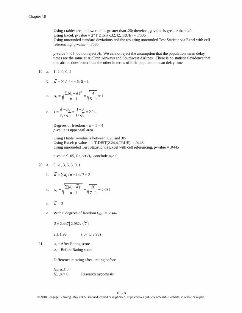
Chapter 10
10 - 8 © 2018 Cengage Learning. May not be scanned, copied or duplicated, or posted to a publicly accessible website, in whole or in part.
Using t table: area in lower tail is greater than .20; therefore, p-value is greater than .40. Using Excel: p-value = 2*T.DIST(-.32,42,TRUE) = .7506 Using unrounded standard deviations and the resulting unrounded Test Statistic via Excel with cell
referencing, p-value = .7535 p-value > .05, do not reject H0. We cannot reject the assumption that the population mean delay
times are the same at AirTran Airways and Southwest Airlines. There is no statisticalevidence that one airline does better than the other in terms of their population mean delay time.
19. a. 1, 2, 0, 0, 2 b. d d ni= ∑ = =/ /5 5 1
c. s d dnd
i=∑ −
−=
−=
( )2
14
5 11
d. t ds n
d
d
=−
=−
=µ
/ /.1 0
1 52 24
Degrees of freedom = n – 1 = 4
p-value is upper-tail area Using t table: p-value is between .025 and .05 Using Excel: p-value = 1-T.DIST(2.24,4,TRUE) = .0443 Using unrounded Test Statistic via Excel with cell referencing, p-value = .0445 p-value ≤ .05, Reject H0; conclude µd> 0. 20. a. 3, -1, 3, 5, 3, 0, 1 b. d d ni= ∑ = =/ /14 7 2
c. 2( ) 26 2.082
1 7 1i
dd d
sn
∑ −= = =
− −
d. d = 2 e. With 6 degrees of freedom t.025 = 2.447 ( )2 2.447 2.082 / 7± 2 ± 1.93 (.07 to 3.93) 21. 1x = After Rating score 2x = Before Rating score Difference = rating after - rating before H0: µd≤ 0 Ha: µd> 0 Research hypothesis
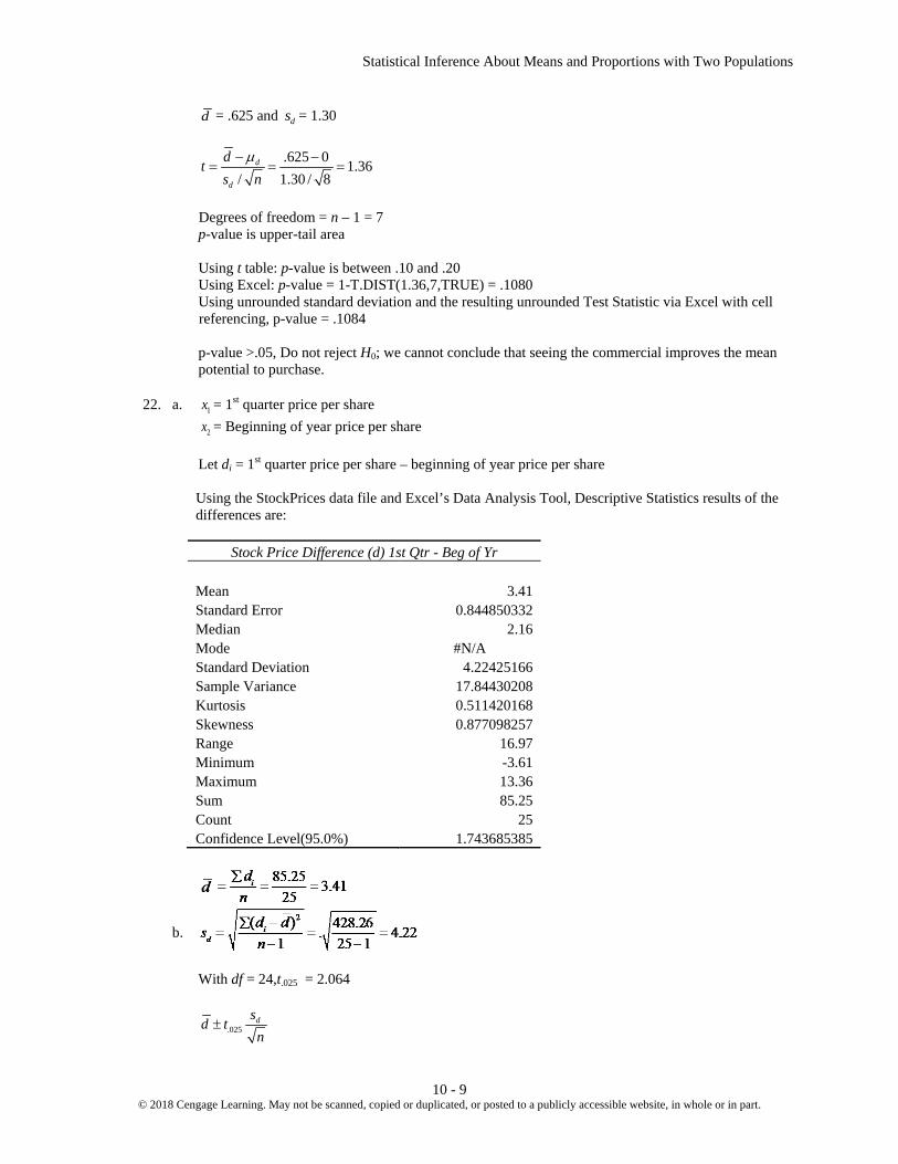
Statistical Inference About Means and Proportions with Two Populations
10 - 9 © 2018 Cengage Learning. May not be scanned, copied or duplicated, or posted to a publicly accessible website, in whole or in part.
d = .625 and sd = 1.30
.625 0 1.36/ 1.30 / 8
d
d
dts n
µ− −= = =
Degrees of freedom = n – 1 = 7
p-value is upper-tail area Using t table: p-value is between .10 and .20 Using Excel: p-value = 1-T.DIST(1.36,7,TRUE) = .1080 Using unrounded standard deviation and the resulting unrounded Test Statistic via Excel with cell
referencing, p-value = .1084 p-value >.05, Do not reject H0; we cannot conclude that seeing the commercial improves the mean
potential to purchase. 22. a. 1x = 1st quarter price per share 2x = Beginning of year price per share Let di = 1st quarter price per share – beginning of year price per share Using the StockPrices data file and Excel’s Data Analysis Tool, Descriptive Statistics results of the
differences are:
Stock Price Difference (d) 1st Qtr - Beg of Yr
Mean 3.41 Standard Error 0.844850332 Median 2.16 Mode #N/A Standard Deviation 4.22425166 Sample Variance 17.84430208 Kurtosis 0.511420168 Skewness 0.877098257 Range 16.97 Minimum -3.61 Maximum 13.36 Sum 85.25 Count 25 Confidence Level(95.0%) 1.743685385
b.
With df = 24,t.025 = 2.064
.025dsd tn
±

Chapter 10
10 - 10 © 2018 Cengage Learning. May not be scanned, copied or duplicated, or posted to a publicly accessible website, in whole or in part.
3.41 ± 2.064
Confidence interval: $3.41 ± $1.74 ($1.67 to $5.15) The 95% confidence interval shows that the population mean price per share of stock hasincreased
between $1.67 and $5.15 over the three-month period. Note that at the beginning of year
With this as the sample mean price per share of stock at the beginning of 2012, the confidence
interval ($1.67 to $5.15) indicates the percentage change in the populationmean price per share of stock would have increased from
1.67/46.13 = .036, or 3.6% to 5.15/46.13 = .112, or 11.2% Thus, for the population of stocks, the mean price per share has increase between 3.6% and 11.2%
over the three-month period. This was excellent news for the 1st quarter of 2012. Stock prices were having one of the largest quarterly increases in years. Theoutlook for a recovering economy was very good at the end of the 1st quarter of 2012.
24. a. 1x = Current Year Airfare
2x = Previous Year Airfare Difference = Current Year Airfare – Previous Year Airfare H0: ≤ 0 Ha: > 0 Research hypothesis Using the BusinessTravel data file and Excel’s Data Analysis Tool, Descriptive Statistics and Paired
t test results are: d
Difference
30
t-Test: Paired Two Sample for Means 63
Mean 23
-42
Standard Error 11.199973
Current Year Previous Year 10
Median 30
Mean 487 464
10
Mode 30
Variance 23238 18508.54545 -27
Standard Dev 38.797844
Observations 12 12
50
Sample Var 1505.2727
Hypothesized Mean Diff 0 60
Kurtosis -1.167691
df 11
60
Skewness -0.575146
t Stat 2.053576389 -30
Range 105
P(T<=t) one-tail 0.032288261
62
Minimum -42
t Critical one-tail 1.795884819 30
Maximum 63
P(T<=t) two-tail 0.064576523
Sum 276
t Critical two-tail 2.20098516
Count 12
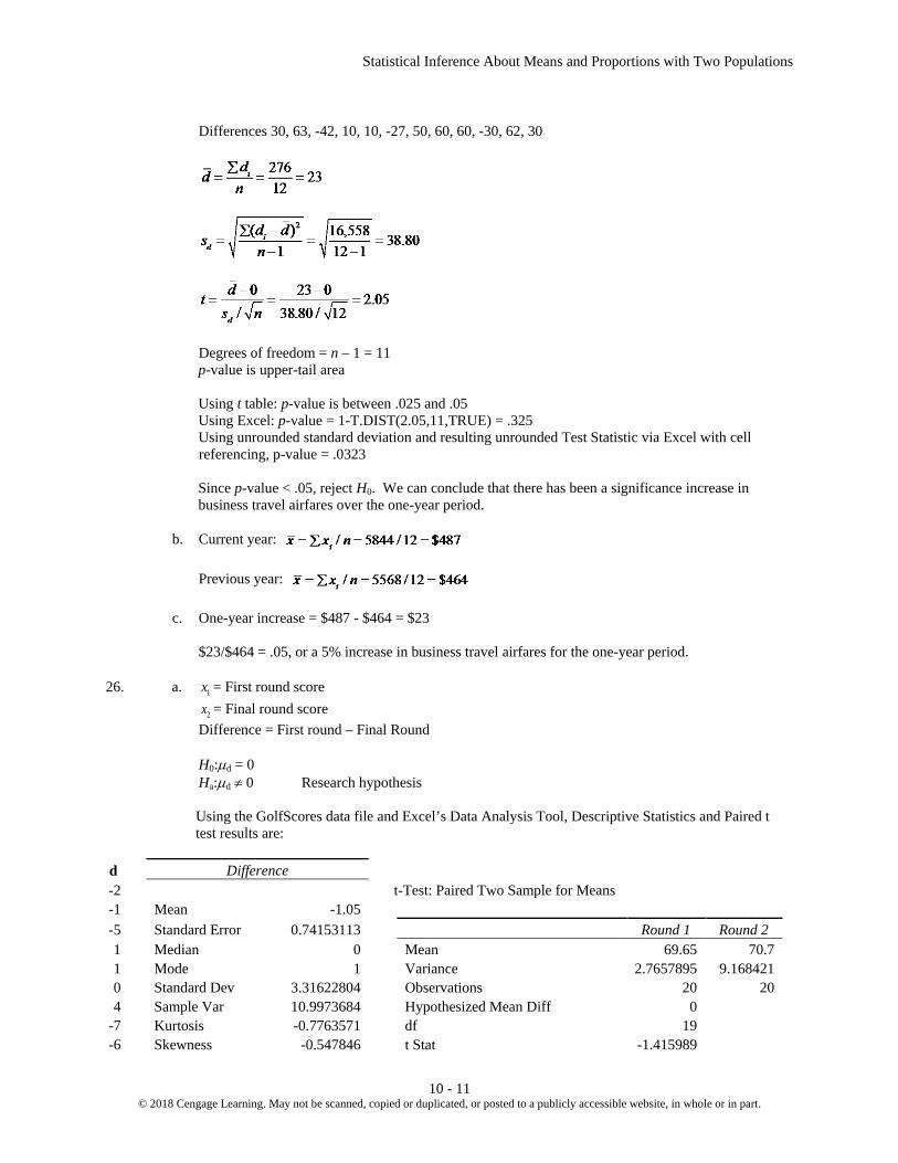
Statistical Inference About Means and Proportions with Two Populations
10 - 11 © 2018 Cengage Learning. May not be scanned, copied or duplicated, or posted to a publicly accessible website, in whole or in part.
Differences 30, 63, -42, 10, 10, -27, 50, 60, 60, -30, 62, 30
Degrees of freedom = n – 1 = 11
p-value is upper-tail area Using t table: p-value is between .025 and .05 Using Excel: p-value = 1-T.DIST(2.05,11,TRUE) = .325 Using unrounded standard deviation and resulting unrounded Test Statistic via Excel with cell
referencing, p-value = .0323 Since p-value < .05, reject H0. We can conclude that there has been a significance increase in
business travel airfares over the one-year period. b. Current year:
Previous year: c. One-year increase = $487 - $464 = $23 $23/$464 = .05, or a 5% increase in business travel airfares for the one-year period.
26. a. 1x = First round score 2x = Final round score Difference = First round – Final Round H0:µd = 0 Ha:µd ≠ 0 Research hypothesis Using the GolfScores data file and Excel’s Data Analysis Tool, Descriptive Statistics and Paired t
test results are:
d
Difference -2
t-Test: Paired Two Sample for Means
-1
Mean -1.05 -5
Standard Error 0.74153113
Round 1 Round 2
1
Median 0
Mean 69.65 70.7 1
Mode 1
Variance 2.7657895 9.168421
0
Standard Dev 3.31622804
Observations 20 20 4
Sample Var 10.9973684
Hypothesized Mean Diff 0
-7
Kurtosis -0.7763571
df 19 -6
Skewness -0.547846
t Stat -1.415989

Chapter 10
10 - 12 © 2018 Cengage Learning. May not be scanned, copied or duplicated, or posted to a publicly accessible website, in whole or in part.
1
Range 11
P(T<=t) one-tail 0.0864819 0
Minimum -7
t Critical one-tail 1.3277282
2
Maximum 4
P(T<=t) two-tail 0.1729638 -3
Sum -21
t Critical two-tail 1.7291328
-7
Count 20 -2
3 1 2 1 -4 Differences: -2, -1, -5, 1, 1, 0, 4, -7, -6, 1, 0, 2, -3, -7, -2, 3, 1, 2, 1, -4
/ 21/ 20 1.05id d n= ∑ = − = −
2( )
3.31621
id
d ds
n∑ −
= =−
1.05 0 1.42/ 3.3162 / 20
d
d
dt
s nµ− − −
= = = −
Degrees of freedom = n – 1 = 19
Because t< 0, p-value is two times the lower tail area Using t table: area in lower tail is between .05 and .10; therefore, p-value isbetween .10 and .20. Using Excel: p-value = 2*T.DIST(-1.42,19,TRUE) = .1717 Using unrounded standard deviation and resulting unrounded Test Statistic via Excel with cell
referencing, p-value = .1730 p-value >.10; Cannot reject H0. There is no significant difference between the mean scores for the
first and fourth rounds. b. d = -1.05; First round scores were lower than fourth round scores. c. α = .10 df = 19 t = 1.729
Margin of error = .05dstn
= = 3.31621.729 1.2820
=
Yes, just check to see if the 90% confidence interval includes a difference of zero. If it does, the
difference is not statistically significant. 90% Confidence interval: -1.05 ± 1.28 (-2.33, .23) The interval does include 0, so the difference is not statistically significant.

Statistical Inference About Means and Proportions with Two Populations
10 - 13 © 2018 Cengage Learning. May not be scanned, copied or duplicated, or posted to a publicly accessible website, in whole or in part.
28. a. 1 2p p− = .48 - .36 = .12
b. 1 1 2 21 2 .05
1 2
(1 ) (1 )p p p pp p zn n− −
− ± +
.48(1 .48) .36(1 .36).12 1.645400 300
− −± +
.12 ± .0614 (.0586 to .1814)
c. .48(1 .48) .36(1 .36).12 1.96400 300
− −± +
.12 ± .0731 (.0469 to .1931)
29. a. 1 1 2 2
1 2
200(.22) 300(.16) .1840200 300
n p n ppn n
+ += = =
+ +
( ) ( )
1 2
1 2
.22 .16 1.701 11 1 .1840 1 .18401 200 300
p pz
p pn n
− −= = =
− +− +
p-value is upper-tail area
Using normal table with z = 1.70: p-value = 1.0000 - .9554 = .0446 Using Excel: p-value = 1-NORM.S.DIST(1.70,TRUE) = .0446 Using unrounded Test Statistic via Excel with cell referencing, p-value = .0449 b. p-value ≤ .05; reject H0. 30. Let p1 = the population proportion of executives in Current survey thinking favorable outlook
p2 = the population proportion of executives in Prior Year survey thinking favorable outlook 1p = 220/400 = .55 2p = 192/400 = .48
1 1 2 21 2 .025
1 2
(1 ) (1 )p p p pp p zn n− −
− ± +
.55(1 .55) .48(1 .48).55 .48 1.96400 400
− −− ± +
.07 ± .0691 (.0009 to .1391) 7% more executives are predicting an increase in full-time jobs. The confidence interval shows the
difference may be from 0% to 14%.
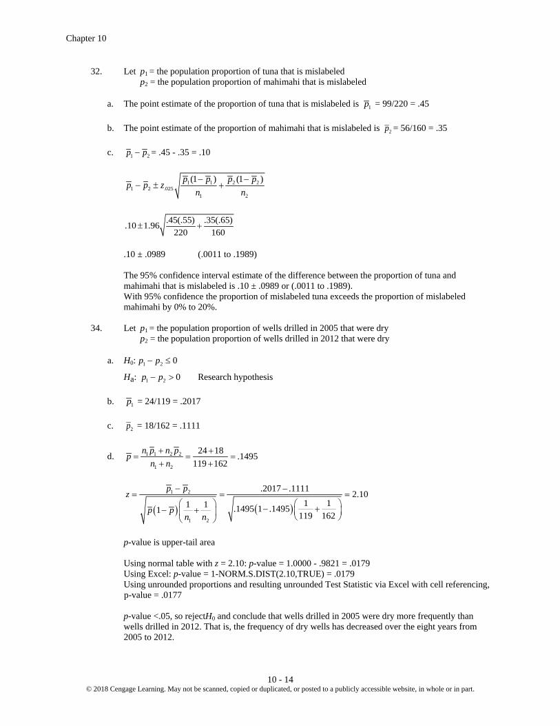
Chapter 10
10 - 14 © 2018 Cengage Learning. May not be scanned, copied or duplicated, or posted to a publicly accessible website, in whole or in part.
32. Let p1 = the population proportion of tuna that is mislabeled p2 = the population proportion of mahimahi that is mislabeled a. The point estimate of the proportion of tuna that is mislabeled is 1p = 99/220 = .45 b. The point estimate of the proportion of mahimahi that is mislabeled is 2p = 56/160 = .35 c. 1 2p p− = .45 - .35 = .10
1 1 2 21 2 .025
1 2
(1 ) (1 )p p p pp p zn n− −
− ± +
.45(.55) .35(.65).10 1.96220 160
± +
.10 ± .0989 (.0011 to .1989) The 95% confidence interval estimate of the difference between the proportion of tuna and
mahimahi that is mislabeled is .10 ± .0989 or (.0011 to .1989). With 95% confidence the proportion of mislabeled tuna exceeds the proportion of mislabeled
mahimahi by 0% to 20%. 34. Let p1 = the population proportion of wells drilled in 2005 that were dry p2 = the population proportion of wells drilled in 2012 that were dry a. H0: 1 2 0p p− ≤
Ha: 1 2 0p p− > Research hypothesis b. 1p = 24/119 = .2017 c. 2p = 18/162 = .1111
d. 1 1 2 2
1 2
24 18 .1495119 162
n p n ppn n
+ += = =
+ +
( ) ( )
1 2
1 2
.2017 .1111 2.101 11 1 .1495 1 .14951 119 162
p pz
p pn n
− −= = =
− +− +
p-value is upper-tail area
Using normal table with z = 2.10: p-value = 1.0000 - .9821 = .0179 Using Excel: p-value = 1-NORM.S.DIST(2.10,TRUE) = .0179 Using unrounded proportions and resulting unrounded Test Statistic via Excel with cell referencing,
p-value = .0177 p-value <.05, so rejectH0 and conclude that wells drilled in 2005 were dry more frequently than
wells drilled in 2012. That is, the frequency of dry wells has decreased over the eight years from 2005 to 2012.

Statistical Inference About Means and Proportions with Two Populations
10 - 15 © 2018 Cengage Learning. May not be scanned, copied or duplicated, or posted to a publicly accessible website, in whole or in part.
36. a. Let = population proportion of rooms occupied for current year = population proportion of rooms occupied for previous year H0: Ha: Research hypothesis b. 1p = 1470/1750 = .84 (current year) 2p = 1458/1800 = .81 (previous year)
c.
p-value is upper-tail area
Using normal table with z = 2.35: p-value = 1.0000 - .9906 = .0094 Using Excel: p-value = 1-NORM.S.DIST(2.35,TRUE) = .0094 Using unrounded pooled proportion and resulting unrounded Test Statistic via Excel with cell
referencing, p-value = .0094 p-value ≤ .05, reject H0. There has been an increase in the hotel occupancy rate.
d. 1 1 2 21 2 .025
1 2
(1 ) (1 )p p p pp p zn n− −
− ± +
.03 ± .025 (.005 to .055)
Officials would likely be pleased with the occupancy statistics. The trend for the current year is an increase in hotel occupancy rates compared to last year. The point estimate is a 3% increase with a 95% confidence interval from .5% to 5.5%.
38. H0: µ1 - µ2 = 0 Ha: µ1 - µ2≠ 0 Research hypothesis
1 2 0
2 2 2 21 2
1 2
( ) (4.1 3.4) 0 2.79(2.2) (1.5)120 100
x x Dz
n nσ σ
− − − −= = =
++
Because z> 0, p-value is two times the upper tail area
Using normal table with z = 2.79: p-value = 2(1 - .9974) = .0052 Using Excel: p-value = 2*(1-NORM.S.DIST(2.79,TRUE)) = .0052

Chapter 10
10 - 16 © 2018 Cengage Learning. May not be scanned, copied or duplicated, or posted to a publicly accessible website, in whole or in part.
Using unrounded Test Statistic via Excel with cell referencing, p-value = .0052 p-value ≤ .05, reject H0. A difference exists with system B having the lower mean checkout time. 40. 1µ = population mean return of Load funds 2µ = population mean return of No Load funds a. 0 1 2: 0H µ µ− ≤ 1 2: 0aH µ µ− > Research hypothesis b. Using the Mutual data file and Excel’s Data Analysis Tool, the Two Sample t-Test with Unequal
Variances results are:
t-Test: Two-Sample Assuming Unequal Variances
Load Return No Load Return Mean 16.22566667 15.70466667 Variance 12.38831506 10.98724644 Observations 30 30 Hypothesized Mean Difference 0
df 58 t Stat 0.590224625 P(T<=t) one-tail 0.278666388 t Critical one-tail 1.671552762 P(T<=t) two-tail 0.557332776 t Critical two-tail 2.001717484
n1 = 30 n2 = 30 x1 = 16.226 x2 = 15.705 s1 = 3.52 s2 = 3.31
1 2 0
2 2 2 21 2
1 2
( ) (16.226 15.705) 0 .59(3.52) (3.31)
30 30
x x Dt
s sn n
− − − −= = =
++
22 2 2 21 2
1 22 2 2 22 2 2 2
1 2
1 1 2 2
3.52 3.3130 30
57.81 3.52 1 3.311 129 30 29 301 1
s sn n
dfs s
n n n n
+ +
= = =
++ − −
Degrees of freedom = 57
p-value is upper-tail area Using t table: p-value is greater than .20 Using Excel: p-value = 1-T.DIST(.59,57,TRUE) = .2788 Using unrounded meansand standard deviations and the resulting unrounded Test Statistic via Excel
with cell referencing, p-value = .2787 p-value > .05, do not reject H0. Cannot conclude that the mutual funds with a load have a greater
mean rate of return.

Statistical Inference About Means and Proportions with Two Populations
10 - 17 © 2018 Cengage Learning. May not be scanned, copied or duplicated, or posted to a publicly accessible website, in whole or in part.
42. a. 1x = SAT score for twin raised with No Siblings 2x = SAT score for twin raised with at least one Sibling Let di = SAT score for twin raised with No Siblings – SAT score for twin raised with Siblings Using the Twins data file and Excel’s Data Analysis Tool, Descriptive Statistics results of the
differences are:
No Sibling SAT- Siblings SAT Difference
Mean 14 Standard Error 12.017531 Median 5 Mode 50 Standard Deviation 53.744033 Sample Variance 2888.4211 Kurtosis -0.823395 Skewness 0.4415705 Range 190 Minimum -60 Maximum 130 Sum 280 Count 20
280 1420
idd
n∑
= = =
b. 2( ) 54,880 53.744
1 19i
dd d
sn
∑ −= = =
−
df = n - 1 = 19, t.05 = 1.729
.05dsd tn
± = 53.74414 1.72920
±
14 ± 20.78 (-6.78 to 34.78) c. H0:µd = 0 Ha:µd ≠ 0 Research hypothesis Using the Twins data file and Excel’s Data Analysis Tool, Descriptive Statistics and Paired t test
results are:
t-Test: Paired Two Sample for Means
No Siblings With Siblings Mean 547.5 533.5 Variance 6798.684211 6413.421053

Chapter 10
10 - 18 © 2018 Cengage Learning. May not be scanned, copied or duplicated, or posted to a publicly accessible website, in whole or in part.
Observations 20 20 Hypothesized Mean Difference 0
df 19 t Stat 1.164964745 P(T<=t) one-tail 0.129225848 t Critical one-tail 2.539483191 P(T<=t) two-tail 0.258451697 t Critical two-tail 2.860934606
14 0 1.165/ 53.744 / 20
d
d
dt
s nµ− −
= = =
Degrees of freedom = n – 1 = 19
Because t> 0, p-value is two times the upper tail area Using t table; area in upper tail is between .10 and .20; therefore, p-value is between .20 and .40. Using Excel: p-value = 2*(1-T.DIST(1.165,19,TRUE)) = .2584 Using unrounded standard deviations and resulting unrounded Test Statistic via Excel with cell
referencing, p-value = .2585
p-value > .01, do not reject H0. cannot conclude that there is a difference between the mean scores for theno sibling and with sibling groups.
44. a. H0: p1 - p2 = 0 Ha: p1 - p2≠ 0 Research Hypothesis 1p = 76/400 = .19 2p = 90/900 = .10
1 1 2 2
1 2
76 90 .1277400 900
n p n ppn n
+ += = =
+ +
( ) ( )
1 2
1 2
.19 .10 4.491 11 1 .1277 1 .12771 400 900
p pz
p pn n
− −= = =
− +− +
Because z> 0, p-value is two times the upper tail area
Using normal table with z = 4.49: p-value = 2(1 - 1) ≈ 0 Using Excel: p-value = 2*(1-NORM.S.DIST(4.49,TRUE)) ≈ 0 Using unrounded pooled proportion and resulting unrounded Test Statistic via Excel with cell
referencing, p-value ≈ 0 p-value ≤ .05, Reject H0; there is a difference between claim rates.
b. 1 1 2 21 2 .025
1 2
(1 ) (1 )p p p pp p zn n− −
− ± +
.19(1 .19) .10(1 .10).19 .10 1.96400 900
− −− ± +

Statistical Inference About Means and Proportions with Two Populations
10 - 19 © 2018 Cengage Learning. May not be scanned, copied or duplicated, or posted to a publicly accessible website, in whole or in part.
.09 ± .0432 (.0468 to .1332) Claim rates are higher for single males. 46. Let p1 = the population proportion of American adults under 30 years old
p2 = the population proportion of Americans who are at least 30 years old a. From datafileComputerNews, there are 109 Yes responses for each age group. The total number of
respondents of the under 30 years group is 200, while the 30 and over group hadb150toal respondents.
American adults under 30 years old: 1p = 109/200 = .545 Americans who are at least 30 years old: 2p = 109/150 = .727 b. 1 2 .545 .727 .182p p− = − = −
1 2
.545(1 .545) .727(1 .727) .0506200 150p ps −
− −= + =
Confidence interval: -.182 ± 1.96(.0506) or.-182 ± .0992 (-.2809 to -.0824) c. Since the confidence interval in part (b) does not include 0 and both values are negative, conclude
that the proportion of American adults under 30 years old who use a computer to gain access to news is less than the proportion of Americans who are at least 30 years old that use a computer to gain access to news.

11 - 1 © 2018 Cengage Learning.May not be scanned, copied or duplicated, or posted to a publicly accessible website, in whole or in part.
Chapter 11 Inferences About Population Variances Solutions: 2. s2 = 25, n =20, df = 19 a. For 90% confidence, 2
.05χ = 30.144 and 2.95χ = 10.117
2 2
22 2
/2 1 /2
( 1) ( 1)n s n s
α α
σχ χ −
− −≤ ≤
219(25) 19(25)30.144 10.117
σ≤ ≤
15.76 ≤σ2≤ 46.95 b. For 95% confidence, 2
.025χ = 32.852 and 2.975χ = 8.907
2 2
22 2
/2 1 /2
( 1) ( 1)n s n s
α α
σχ χ −
− −≤ ≤
219(25) 19(25)32.852 8.907
σ≤ ≤
14.46 ≤σ2≤ 53.33
c. 2 2
2 2/2 1 /2
( 1) ( 1)n s n s
α α
σχ χ −
− −≤ ≤
14.46 53.33σ≤ ≤ 3.8≤σ≤ 7.3 4. s2 = .36, n =18, df = 17 a. For 90% confidence, 2
.05χ = 27.587 and 2.95χ = 8.672
2 2
22 2
/2 1 /2
( 1) ( 1)n s n s
α α
σχ χ −
− −≤ ≤
217(.36) 17(.36)27.587 8.672
σ≤ ≤
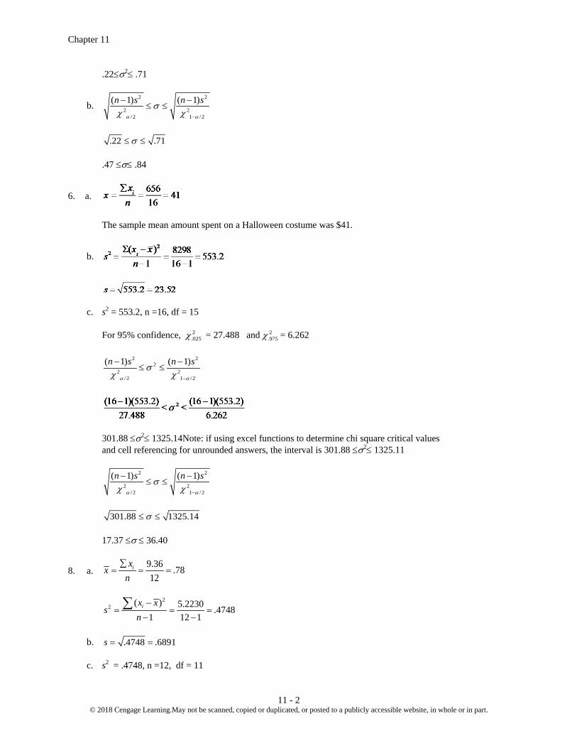
Chapter 11
11 - 2 © 2018 Cengage Learning.May not be scanned, copied or duplicated, or posted to a publicly accessible website, in whole or in part.
.22≤σ2≤ .71
b. 2 2
2 2/2 1 /2
( 1) ( 1)n s n s
α α
σχ χ −
− −≤ ≤
.22 .71σ≤ ≤ .47 ≤σ≤ .84
6. a.
The sample mean amount spent on a Halloween costume was $41.
b.
c. s2 = 553.2, n =16, df = 15 For 95% confidence, 2
.025χ = 27.488 and 2.975χ = 6.262
2 2
22 2
/2 1 /2
( 1) ( 1)n s n s
α α
σχ χ −
− −≤ ≤
301.88 ≤σ2≤ 1325.14Note: if using excel functions to determine chi square critical values and cell referencing for unrounded answers, the interval is 301.88 ≤σ2≤ 1325.11
2 2
2 2/2 1 /2
( 1) ( 1)n s n s
α α
σχ χ −
− −≤ ≤
301.88 1325.14σ≤ ≤ 17.37 ≤σ ≤ 36.40
8. a. 9.36 .7812
ixx
n∑
= = =
2
2 ( ) 5.2230 .47481 12 1
ix xs
n−
= = =− −
∑
b. .4748 .6891s = = c. s2 = .4748, n =12, df = 11
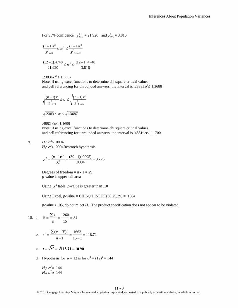
Inferences About Population Variances
11 - 3 © 2018 Cengage Learning.May not be scanned, copied or duplicated, or posted to a publicly accessible website, in whole or in part.
For 95% confidence, 2
.025χ = 21.920 and 2.975χ = 3.816
2 2
22 2
/2 1 /2
( 1) ( 1)n s n s
α α
σχ χ −
− −≤ ≤
2(12 1).4748 (12 1).474821.920 3.816
σ− −≤ ≤
.2383≤σ2 ≤ 1.3687 Note: if using excel functions to determine chi square critical values and cell referencing for unrounded answers, the interval is .2383≤σ2≤ 1.3688
2 2
2 2/2 1 /2
( 1) ( 1)n s n s
α α
σχ χ −
− −≤ ≤
.2383 1.3687σ≤ ≤ .4882 ≤σ≤ 1.1699 Note: if using excel functions to determine chi square critical values and cell referencing for unrounded answers, the interval is .4881≤σ≤ 1.1700 9. H0: σ2≤ .0004 Ha: σ2> .0004Research hypothesis
2
220
( 1) (30 1)(.0005) 36.25.0004
n sχσ− −
= = =
Degrees of freedom = n - 1 = 29 p-value is upper-tail area Using 2χ table, p-value is greater than .10 Using Excel, p-value = CHISQ.DIST.RT(36.25,29) = .1664 p-value > .05, do not reject H0. The product specification does not appear to be violated.
10. a. 1260
8415
ixx
n
∑= = =
b. 2
2 ( ) 1662118.71
1 15 1ix x
sn
−= = =
− −
∑
c. d. Hypothesis for = 12 is for σ2 = (12)2 = 144 H0: σ2= 144 Ha: σ2 144
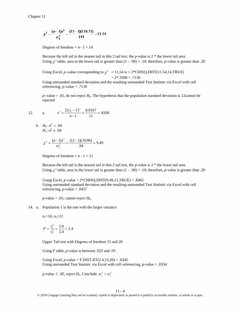
Chapter 11
11 - 4 © 2018 Cengage Learning.May not be scanned, copied or duplicated, or posted to a publicly accessible website, in whole or in part.
Degrees of freedom = n– 1 = 14
Because the left tail is the nearest tail in this 2 tail test, the p-value is 2 * the lower tail area Using 2χ table, area in the lower tail is greater than (1 – .90) = .10; therefore, p-value is greater than .20 Using Excel, p–value corresponding to 2χ = 11.54 is = 2*CHISQ.DIST(11.54,14,TRUE) = 2*.3568 = .7136 Using unrounded standard deviation and the resulting unrounded Test Statistic via Excel with cell
referencing, p-value = .7139 p–value > .05, do not reject H0. The hypothesis that the population standard deviation is 12cannot be
rejected
12. a. 2
2 ( ) 8.9167 .81061 11
ix xs
nΣ −
= = =−
b. H0: σ2 = .94 Ha: σ2 ≠ .94
2
220
( 1) (12 1)(.8106) 9.49.94
n sχσ− −
= = =
Degrees of freedom = n - 1 = 11 Because the left tail is the nearest tail in this 2 tail test, the p-value is 2 * the lower tail area Using 2χ table, area in the lower tail is greater than (1 – .90) = .10; therefore, p-value is greater than .20 Using Excel, p-value = 2*CHISQ.DIST(9.49,11,TRUE) = .8465 Using unrounded standard deviation and the resulting unrounded Test Statistic via Excel with cell
referencing, p-value = .8457 p-value > .05, cannot reject H0. 14. a. Population 1 is the one with the larger variance n1=16, n2=21
2122
5.8 2.42.4
sFs
= = =
Upper Tail test with Degrees of freedom 15 and 20 Using F table, p-value is between .025 and .05 Using Excel, p-value = F.DIST.RT(2.4,15,20) = .0345 Using unrounded Test Statistic via Excel with cell referencing, p-value = .0334 p-value ≤ .05, reject H0. Conclude 2 2
1 2σ σ>

Inferences About Population Variances
11 - 5 © 2018 Cengage Learning.May not be scanned, copied or duplicated, or posted to a publicly accessible website, in whole or in part.
b. Critical F.05 = 2.20 Reject H0 if F ≥ 2.20 2.4 ≥ 2.20, reject H0. Conclude 2 2
1 2σ σ> 15. a. Larger sample variance is 2
1s n1=21, n2=26
2122
8.2 2.054
sFs
= = =
Two Tail test (2 * right tail) with Degrees of freedom 20 and 25 Using F table, area in the upper tail is between .025 and .05; Two-tail p-value is between .05 and .10 Using Excel, p-value = 2*F.DIST.RT(2.05,20,25) = .0904 p-value > .05, do not reject H0. b. Since we have a two-tailed test / 2 .025 2.30F Fα = = Reject H0 if F ≥ 2.30 2.05 < 2.30, do not reject H0. 16. For this type of hypothesis test, we place the larger variance in the numerator. So the Fidelity variance is
given the subscript of 1.s1= 18.9, s2 = 15 2 2
0 1 2:H σ σ≤ 2 2
1 2:aH σ σ> Research hypothesis
2 212 22
18.9 1.587615.0
sFs
= = =
Upper Tail test; Degrees of freedom in the numerator and denominator arboth 59 Using the F table and estimating with 60 df for each, p-value is between .025 and .05 Using Excel,p-value corresponding to F = 1.5876 is F.DIST.RT(1.5876,59,59) = .0392 p-value ≤ .05, reject H0. We conclude that the Fidelity fund has a greater variance than the American
Century fund and therefore is more risky. 17. a. Population 1 is 4 year old automobiles since it is the one with the larger variance s1= 170, n1=26, s2 = 100, n2=25 2 2
0 1 2:H σ σ≤ 2 2
1 2:aH σ σ> Research hypothesis

Chapter 11
11 - 6 © 2018 Cengage Learning.May not be scanned, copied or duplicated, or posted to a publicly accessible website, in whole or in part.
b. 2 212 22
170 2.89100
sFs
= = =
Upper Tail test; Degrees of freedom 25 and 24 Using F table, p-value is less than .01 Using Excel, p-value = F.DIST.RT(2.89,25,24) = .0057 p-value ≤ .01, reject H0. Conclude that 4 year old automobiles have a larger variance in annual repair costs
compared to 2 year old automobiles. This is expected due to the fact that older automobiles are more likely to have some more expensive repairs which lead to greater variance in the annual repair costs.
18. We place the larger sample variance in the numerator. So, the Merrill Lynch variance is given the subscript of 1. s1= 587, n1=16, s2 = 489, n2=10 2 2
0 1 2:H σ σ= 2 2
1 2:aH σ σ≠ Research hypothesis
2 212 22
587 1.44489
sFs
= = =
Two Tail test (2 * right tail) with Degrees of freedom 15 and 9 Using F table, area in the upper tail is greater than .10; Two-tail p-value is greater than .20 Using Excel,p-value corresponding to F = 1.44 is2*F.DIST.RT(1.44,15,9) = .5906 Using unrounded Test Statistic via Excel with cell referencing, p-value = .5898 p-value > .10, do not reject H0. We cannot conclude there is a statistically significant difference between
the variances for the two companies. 20. Population 1 is Managers since it is the one with the larger variance s1
2= 11.1, n1=26, s22 = 2.1, n2=25
2 2
0 1 2:H σ σ= 2 2
1 2:aH σ σ≠
2122
11.1 5.292.1
sFs
= = =
Two Tail test (2 * right tail) with Degrees of freedom 25 and 24 Using F table, area in the upper tail is less than .01; Two-tail p-value is less than .02 Using Excel, p-value = 2*F.DIST.RT(5.29,25,24) = .0001 p-value ≤ .05, reject H0. The population variances are not equal for seniors and managers.

Inferences About Population Variances
11 - 7 © 2018 Cengage Learning.May not be scanned, copied or duplicated, or posted to a publicly accessible website, in whole or in part.
22. a. Since it is the one with the larger variance, Population 1 - Wet pavement. s1 = 32, n1=16, s2 = 16, n2=16 2 2
0 1 2:H σ σ≤ 2 2
1 2:aH σ σ> Research hypothesis
2 212 22
32 4.0016
sFs
= = =
Upper Tail test; Degrees of freedom 15 and 15 Using F table, p-value is less than .01 Using Excel, p-value = F.DIST.RT(4.00,15,15) = .0054 p-value ≤ .05, reject H0. Conclude that there is greater variability in stopping distances on wet pavement. b. Drive carefully on wet pavement because of the uncertainty in stopping distances. 24. s = 14.95, n =13, df = 12 For 95% confidence, 2
.025χ = 23.337 and 2.975χ = 4.404
2 2
22 2
/2 1 /2
( 1) ( 1)n s n s
α α
σχ χ −
− −≤ ≤
2 2
2(12)(14.95) (12)(14.95)23.337 4.404
σ≤ ≤
114.9 ≤σ2≤ 609
2 2
2 2/2 1 /2
( 1) ( 1)n s n s
α α
σχ χ −
− −≤ ≤
114.9 609σ≤ ≤ 10.72 ≤σ≤ 24.68 26. a. s = .014, n =15, df = 14 H0: σ2≤ .0001 Ha: σ2 > .0001 Research hypothesis
2 2
22
( 1) (15 1)(.014) 27.44.0001o
n sχσ− −
= = =
Degrees of freedom = n - 1 = 14 p-value is upper-tail area Using 2χ table, p- value is between .01 and .025

Chapter 11
11 - 8 © 2018 Cengage Learning.May not be scanned, copied or duplicated, or posted to a publicly accessible website, in whole or in part.
Using Excel, p-value = CHISQ.DIST.RT(27.44,14) = .0169 p-value ≤ .10, reject H0. Variance exceeds maximum variance requirement. b. For 90% confidence, df=14, 2
.05χ = 23.685 and 2.95χ = 6.571
2 2
22 2
/2 1 /2
( 1) ( 1)n s n s
α α
σχ χ −
− −≤ ≤
2 2
2(14)(.014) (14)(.014)23.685 6.571
σ≤ ≤
.00012 ≤σ2≤ .00042 28. s2 = 1.5, n =22, df = 21 H0: σ2 ≤ 1 Ha: σ2 > 1
2
220
( 1) (22 1)(1.5) 31.501
n sχσ− −
= = =
Degrees of freedom = n - 1 = 21 p-value is upper-tail area Using 2χ table, p-value is between .05 and .10 Using Excel, p-value = CHISQ.DIST.RT(31.50,21) = .0657 p-value ≤ .10, reject H0. Conclude that σ2> 1. 30. a. Try n = 15 with s = 8, For 95% confidence, df = 14 2
.025χ = 26.119 and 2.975χ = 5.629
2 2
22 2
/2 1 /2
( 1) ( 1)n s n s
α α
σχ χ −
− −≤ ≤
2(14)(64) (14)(64)26.119 5.629
σ≤ ≤
34.3 ≤σ2≤ 159.2
2 2
2 2/2 1 /2
( 1) ( 1)n s n s
α α
σχ χ −
− −≤ ≤
34.3 159.2σ≤ ≤ 5.86 ≤σ≤ 12.62 Therefore, a sample size of 15 was used.

Inferences About Population Variances
11 - 9 © 2018 Cengage Learning.May not be scanned, copied or duplicated, or posted to a publicly accessible website, in whole or in part.
b. n = 25; expect the width of the interval to be smaller. For 95% confidence, df = 24 2
.05χ = 39.364 and 2.975χ = 12.401
2 2
22 2
/2 1 /2
( 1) ( 1)n s n s
α α
σχ χ −
− −≤ ≤
2 2
2(24)(8) (24)(8)39.364 12.401
σ≤ ≤
39.02 ≤σ2≤123.86
2 2
2 2/2 1 /2
( 1) ( 1)n s n s
α α
σχ χ −
− −≤ ≤
39.02 123.86σ≤ ≤ 6.25 ≤σ≤ 11.13 32. 2 2
0 1 2:H σ σ= 2 2
1 2:aH σ σ≠ Research hypothesis Since it is the one with the larger variance, population 1 is those who completed course s1 = .940, n1=352, s2 = .797, n2=73 Using critical value approach and Excel to determine the critical value, since F tables do not have 351 and
72 degrees of freedom. Using Excel, F.INV.RT(0.025,351,72) gives the Critical F.025 = 1.466 Reject H0 if F ≥ 1.466
2 212 22
.940 1.39
.797sFs
= = =
F< 1.466, do not reject H0. We are not able to conclude students who complete the course and students who
drop out have different variances of grade point averages. Using Excel, the pvalue approach gives the following: Two Tail test (2 * right tail) with Degrees of freedom 351 and 72 Using Excel: p-value = 2*F.DIST.RT(1.39,351,72) = .0906 Using unrounded Test Statistic via Excel with cell referencing, p-value = .0899 p-value > .05, do not reject 0H . There is not a statistically significant difference in the variances.

Chapter 11
11 - 10 © 2018 Cengage Learning.May not be scanned, copied or duplicated, or posted to a publicly accessible website, in whole or in part.
34. 2 20 1 2:H σ σ=
2 21 2:aH σ σ≠
2122
25 2.0812
sFs
= = =
Two Tail test (2 * right tail) with Degrees of freedom 30 and 24 Using F table, area in tail is between .025 and .05; Two-tail p-value is between .05 and .10 Using Excel, p-value = 2*F.DIST.RT(2.08,30,24) = .0695 Using unrounded Test Statistic via Excel with cell referencing, p-value = .0689 p-value ≤ .10, reject H0. Conclude that the population variances are not equal.

12 - 1 © 2018 Cengage Learning. May not be scanned, copied or duplicated, or posted to a publicly accessible website, in whole or in part.
Chapter 12 Tests of Goodness of Fit and Independence Solutions: 1. a. Expected frequencies: e1 = 200 (.40) = 80, e2 = 200 (.40) = 80 e3 = 200 (.20) = 40 Actual frequencies: f1 = 60, f2 = 120, f3 = 20
2
2 ( )i i
i
f ee
χ−
= ∑
2 2 22 (60 80) (120 80) (20 40)
80 80 40400 1600 40080 80 40
5 20 1035
χ − − −= + +
= + +
= + +=
k - 1 = 2 degrees of freedom Using the 2χ table with df = 2, 2χ = 35 shows the p-value is less than .005. Using Excel, the p-value corresponding to 2χ = 35; = CHISQ.DIST.RT(35,2) = .0000 p-value ≤ .01, reject H0 b. For 2 degrees of freedom, .01χ = 9.210 Reject H0 if 2χ ≥ 9.210 2χ = 35, reject H0 2. Expected frequencies: e1 = 300 (.25) = 75, e2 = 300 (.25) = 75 e3 = 300 (.25) = 75, e4 = 300 (.25) = 75 Actual frequencies: f1 = 85, f2 = 95, f3 = 50, f4 = 70
2
2 ( )i i
i
f ee
χ−
= ∑

Chapter 12
12 - 2 © 2018 Cengage Learning. May not be scanned, copied or duplicated, or posted to a publicly accessible website, in whole or in part.
2 2 2 22 (85 75) (95 75) (50 75) (70 75)
75 75 75 75100 400 625 2575 75 75 75
115075
15.33
χ − − − −= + + +
= + + +
=
=
k - 1 = 3 degrees of freedom Using the 2χ table with df = 3, 2χ = 15.33 shows the p-value is less than .005. Using Excel, the p-value corresponding to 2χ = 15.33;= CHISQ.DIST.RT(15.33,3) = .0016. p-value ≤ .05, reject H0 The population proportions are not the same. 3. H0 = pABC = .29, pCBS = .28, pNBC = .25, pIND = .18 Ha = The proportions are not pABC = .29, pCBS = .28, pNBC = .25, pIND = .18 Expected frequencies: 300 (.29) = 87, 300 (.28) = 84 300 (.25) = 75, 300 (.18) = 54 e1 = 87, e2 = 84, e3 = 75, e4 = 54 Actual frequencies: f1 = 95, f2 = 70, f3 = 89, f4 = 46
2
2 ( )i i
i
f ee
χ−
= ∑
2 2 2 22 (95 87) (70 84) (89 75) (46 54)
87 84 75 546.87
χ − − − −= + + +
=
k - 1 = 3 degrees of freedom Using the 2χ table with df = 3, 2χ = 6.87 shows the p-value is between .05 and .10. Using Excel, the p-value corresponding to 2χ = 6.87;= CHISQ.DIST.RT(6.87,3) = .0762. p-value > .05, do not reject H0. There has not been a significant change in the viewing audience
proportions.
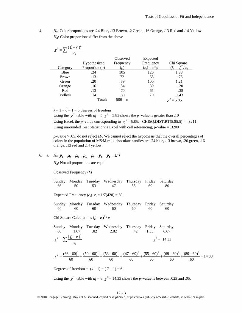
Tests of Goodness of Fit and Independence
12 - 3 © 2018 Cengage Learning. May not be scanned, copied or duplicated, or posted to a publicly accessible website, in whole or in part.
4. H0: Color proportions are .24 Blue, .13 Brown, .2 Green, .16 Orange, .13 Red and .14 Yellow Ha: Color proportions differ from the above
2
2 ( )i i
i
f ee
χ−
= ∑
Observed Expected Hypothesized Frequency Frequency Chi Square
Category Proportion (p) (fi) (ei) = n*p (fi – ei)2 / ei Blue .24 105 120 1.88
Brown .13 72 65 .75 Green .20 89 100 1.21
Orange .16 84 80 .20 Red .13 70 65 .38
Yellow .14 80 70 1.43 Total: 500 = n 2χ = 5.85
k – 1 = 6 – 1 = 5 degrees of freedom Using the 2χ table with df = 5, 2χ = 5.85 shows the p–value is greater than .10 Using Excel, the p–value corresponding to 2χ = 5.85;= CHISQ.DIST.RT(5.85,5) = .3211 Using unrounded Test Statistic via Excel with cell referencing, p-value = .3209 p–value > .05, do not reject H0. We cannot reject the hypothesis that the overall percentages of
colors in the population of M&M milk chocolate candies are .24 blue, .13 brown, .20 green, .16 orange, .13 red and .14 yellow.
6. a. H0:
Ha: Not all proportions are equal Observed Frequency (fi) Sunday Monday Tuesday Wednesday Thursday Friday Saturday 66 50 53 47 55 69 80 Expected Frequency (ei) ei = 1/7(420) = 60 Sunday Monday Tuesday Wednesday Thursday Friday Saturday 60 60 60 60 60 60 60 Chi Square Calculations (fi – ei)2 / ei Sunday Monday Tuesday Wednesday Thursday Friday Saturday .60 1.67 .82 2.82 .42 1.35 6.67
2
2 ( )i i
i
f ee
χ−
= ∑ 2χ = 14.33
2 2 2 2 2 2 2
2 (66 60) (50 60) (53 60) (47 60) (55 60) (69 60) (80 60) 14.3360 60 60 60 60 60 60
χ − − − − − − −= + + + + + + =
Degrees of freedom = (k – 1) = ( 7 – 1) = 6 Using the 2χ table with df = 6, 2χ = 14.33 shows the p–value is between .025 and .05.

Chapter 12
12 - 4 © 2018 Cengage Learning. May not be scanned, copied or duplicated, or posted to a publicly accessible website, in whole or in part.
Using Excel, the p–value corresponding to 2χ = 14.33;= CHISQ.DIST.RT(14.33,6) = .0262 Using unrounded Test Statistic via Excel with cell referencing, p-value = .0261
p–value ≤ .05, reject H0. Conclude the proportion of traffic accidents is not the same for each day of the week.
b. Percentage of traffic accidents by day of the week Sunday 66/420 = .1571 15.71% Monday 50/420 = .1190 11.90% Tuesday 53/420 = .1262 12.62% Wednesday 47/420 = .1119 11.19% Thursday 55/420 = .1310 13.10% Friday 69/420 = .1643 16.43% Saturday 80/420 = .1905 19.05%
Saturday has the highest percentage of traffic accident (19%). Saturday is typically the late night and more social day/evening of the week. Alcohol, speeding and distractions are more likely to affect driving on Saturdays. Friday is the second highest with 16.43%.
7. H0:The column variable is independent of the row variable Ha: The column variable is not independent of the row variable
Observed Frequencies (fij)
A B C Total P 20 44 50 114 Q 30 26 30 86 Total 50 70 80 200
Expected Frequencies (eij)( )( )
ij
i jRow Total Column Totale
SampleSize=
A B C Total P 28.5 39.9 45.6 114 Q 21.5 30.1 34.4 86 Total 50 70 80 200
Chi–Square Calculations (fij–eij)2/ eij
A B C Total P 2.54 .42 .42 3.38 Q 3.36 .56 .56 4.48
2χ = 7.86 2
2 ( )i i
i
f ee
χ−
= ∑
Degrees of freedom = (r – 1)(c – 1) = (2–1)(3–1) = 2 Using the 2χ table with df = 2, 2χ = 7.86 shows the p–value is between .01 and .025. Using Excel, the p–value corresponding to 2χ = 7.86;= CHISQ.DIST.RT(7.86,2) =.0196. p–value ≤ .05, reject H0. Conclude that there is an association between the column variable andthe
row variable. The variables are not independent. 8. H0:The column variable is independent of the row variable

Tests of Goodness of Fit and Independence
12 - 5 © 2018 Cengage Learning. May not be scanned, copied or duplicated, or posted to a publicly accessible website, in whole or in part.
Ha: The column variable is not independent on the row variable Observed Frequencies (fij)
A B C Total P 20 30 20 70 Q 30 60 25 115 R 10 15 30 55 Total 60 105 75 240
Expected Frequencies (eij)( )( )
ij
i jRow Total Column Totale
SampleSize=
A B C Total P 17.50 30.63 21.88 70 Q 28.75 50.31 35.94 115 R 13.75 24.06 17.19 55 Total 60 105 75 240
Chi–Square Calculations (fij–eij)2 / eij
A B C Total P .36 .01 .16 .53 Q .05 1.87 3.33 5.25 R 1.02 3.41 9.55 13.99
2χ = 19.77 2
2 ( )i i
i
f ee
χ−
= ∑
Degrees of freedom = (r – 1)(c – 1) = (3 – 1)(3– 1) = 4 Using the 2χ table with df = 4, 2χ = 19.77 shows the p–value is less than .005. Using Excel, the p–value corresponding to 2χ = 19.77;= CHISQ.DIST.RT(19.77,4) = .0006. p–value ≤ .05, reject H0. Conclude that the column variable is not independent of the row variable. 9. a. H0: Type of ticket purchased is independent of the type of flight Ha: Type of ticket purchased is not independent of the type of flight
Expected Frequencies:( )( )
ij
i jRow Total Column Totale
SampleSize=
e11 = 35.59 e12 = 15.41 e21 = 150.73 e22 = 65.27 e31 = 455.68 e32 = 197.32
Observed Expected Frequency Frequency Chi–square
Ticket Flight (fi) (ei) (fi – ei)2 / ei
First Domestic 29 35.59 1.22 First International 22 15.41 2.82
Business Domestic 95 150.73 20.61

Chapter 12
12 - 6 © 2018 Cengage Learning. May not be scanned, copied or duplicated, or posted to a publicly accessible website, in whole or in part.
Business International 121 65.27 47.59 Full Fare Domestic 518 455.68 8.52 Full Fare International 135 197.32 19.68
Totals: 920 100.43 Degrees of freedom = (r – 1)(c – 1) = (3 – 1)(2 – 1) = 2 Using the 2χ table with df = 2, 2χ = 100.43 shows the p–value is less than .005. Using Excel, the p–value corresponding to 2χ = 100.43;= CHISQ.DIST.RT(100.43,2) = .0000. p–value ≤ .05, reject H0. Conclude that the type of ticket purchased is not independent of the type of
flight. We can expect the type of ticket purchased to depend upon whether the flight is domestic or international.
b. Column Percentages =Ticket&FlightType Frequency/Column Total; For example: 29/642 = .045 =
4.5% Type of Flight Type of Ticket Domestic International First Class 4.5% 7.9% Business Class 14.8% 43.5% Economy Class 80.7% 48.6%
A higher percentage of first class and business class tickets are purchased for international flights compared to domestic flights. Economy class tickets are purchased more for domestic flights. The first class or business class tickets are purchased for more than 50% of the international flights; 7.9% + 43.5% = 51.4%.
10. a. H0: Employment plan is independent of the type of company Ha: Employment plan is not independent of the type of company Observed Frequency (fij)
Employment Plan Private Public Total Add Employees 37 32 69 No Change 19 34 53 Lay Off Employees 16 42 58 Total 72 108 180
Expected Frequency (eij) ( )( )
ij
i jRow Total Column Totale
SampleSize=
Employment Plan Private Public Total Add Employees 27.6 41.4 69 No Change 21.2 31.8 53 Lay Off Employees 23.2 34.8 58 Total 72.0 108.0 180
Chi Square Calculations (fij – eij)2 / eij
Employment Plan Private Public Total
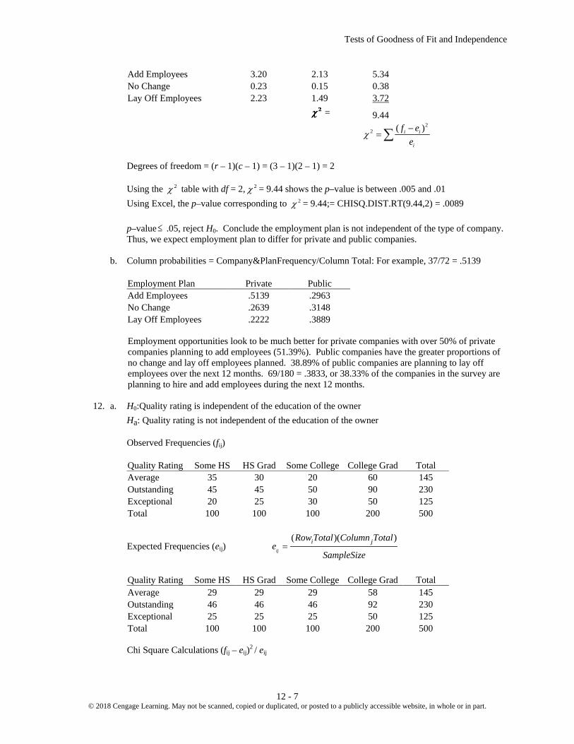
Tests of Goodness of Fit and Independence
12 - 7 © 2018 Cengage Learning. May not be scanned, copied or duplicated, or posted to a publicly accessible website, in whole or in part.
Add Employees 3.20 2.13 5.34 No Change 0.23 0.15 0.38 Lay Off Employees 2.23 1.49 3.72
= 9.44
2
2 ( )i i
i
f ee
χ−
= ∑
Degrees of freedom = (r – 1)(c – 1) = (3 – 1)(2 – 1) = 2 Using the 2χ table with df = 2, 2χ = 9.44 shows the p–value is between .005 and .01 Using Excel, the p–value corresponding to 2χ = 9.44;= CHISQ.DIST.RT(9.44,2) = .0089
p–value ≤ .05, reject H0. Conclude the employment plan is not independent of the type of company. Thus, we expect employment plan to differ for private and public companies.
b. Column probabilities = Company&PlanFrequency/Column Total: For example, 37/72 = .5139
Employment Plan Private Public Add Employees .5139 .2963 No Change .2639 .3148 Lay Off Employees .2222 .3889
Employment opportunities look to be much better for private companies with over 50% of private companies planning to add employees (51.39%). Public companies have the greater proportions of no change and lay off employees planned. 38.89% of public companies are planning to lay off employees over the next 12 months. 69/180 = .3833, or 38.33% of the companies in the survey are planning to hire and add employees during the next 12 months.
12. a. H0:Quality rating is independent of the education of the owner Ha: Quality rating is not independent of the education of the owner Observed Frequencies (fij)
Quality Rating Some HS HS Grad Some College College Grad Total Average 35 30 20 60 145 Outstanding 45 45 50 90 230 Exceptional 20 25 30 50 125 Total 100 100 100 200 500
Expected Frequencies (eij) ( )( )
ij
i jRow Total Column Totale
SampleSize=
Quality Rating Some HS HS Grad Some College College Grad Total Average 29 29 29 58 145 Outstanding 46 46 46 92 230 Exceptional 25 25 25 50 125 Total 100 100 100 200 500
Chi Square Calculations (fij – eij)2 / eij

Chapter 12
12 - 8 © 2018 Cengage Learning. May not be scanned, copied or duplicated, or posted to a publicly accessible website, in whole or in part.
Quality Rating Some HS HS Grad Some College College Grad Total Average 1.24 .03 2.79 .07 4.14 Outstanding .02 .02 .35 .04 .43 Exceptional 1.00 .00 1.00 .00 2.00
2
2 ( )i i
i
f ee
χ−
= ∑
Degrees of freedom = (r – 1)(c – 1) = (3– 1)(4 – 1) = 6 Using the 2χ table with df = 6, 2χ = 6.57 shows the p–value is greater than .10 Using Excel, the p–value corresponding to 2χ = 6.57;= CHISQ.DIST.RT(6.57,6) = .3624 Using unrounded Test Statistic via Excel with cell referencing, p-value = .3622
p–value > .05, do not reject H0. We are unable to conclude that the quality rating is not independent of the education of the owner. Thus, quality ratings are not expected to differ with the education of the owner.
b. Average: 145/500 = 29% Outstanding: 230/500 = 46% Exceptional: 125/500 = 25% New owners look to be pretty satisfied with their new automobiles with almost 50% rating the
quality outstanding and over 70% rating the quality outstanding or exceptional. 14. a. The sample size is very large: 6448 b. H0: Attitude toward building new nuclear power plants is independent of Country Ha:Attitude toward building new nuclear power plants is not independent of Country
Observed Frequency (fij)
Country Response G.B. France Italy Spain Ger. U.S. Total Strongly favor 141 161 298 133 128 204 1065 Favor 348 366 309 222 272 326 1843 Oppose 381 334 219 311 322 316 1883 Strongly Oppose 217 215 219 443 389 174 1657
Total 1087 1076 1045 1109 1111 1020 6448
Expected Frequency (eij) ( )( )
ij
i jRow Total Column Totale
SampleSize=
Country
Response G.B. France Italy Spain Ger. U.S. Total Strongly favor 179.5 177.7 172.6 183.2 183.5 168.5 1065 Favor 310.7 307.5 298.7 317.0 317.6 291.5 1843 Oppose 317.4 314.2 305.2 323.9 324.4 297.9 1883 Strongly Oppose 279.3 276.5 268.5 285.0 285.5 262.1 1657
Total 1087 1076 1045 1109 1111 1020 6448
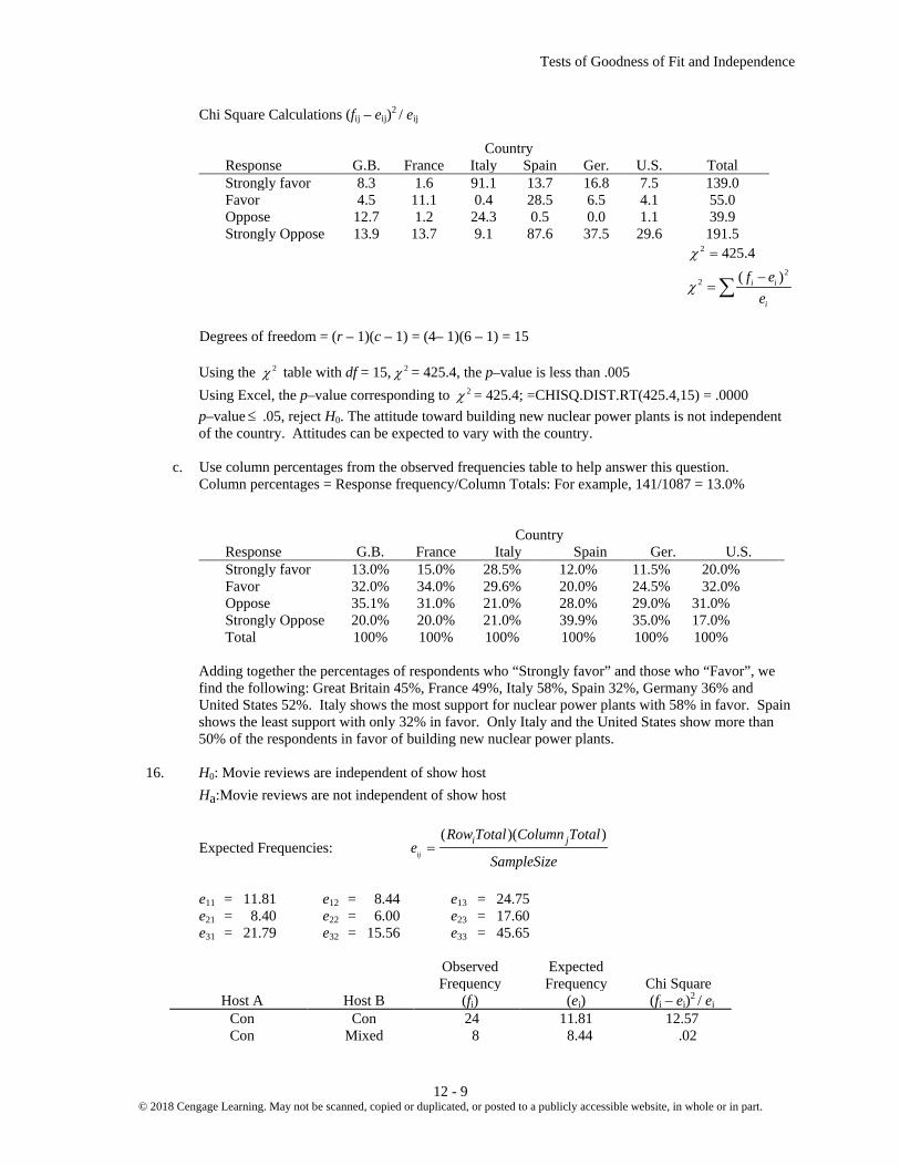
Tests of Goodness of Fit and Independence
12 - 9 © 2018 Cengage Learning. May not be scanned, copied or duplicated, or posted to a publicly accessible website, in whole or in part.
Chi Square Calculations (fij – eij)2 / eij
Country Response G.B. France Italy Spain Ger. U.S. Total Strongly favor 8.3 1.6 91.1 13.7 16.8 7.5 139.0 Favor 4.5 11.1 0.4 28.5 6.5 4.1 55.0 Oppose 12.7 1.2 24.3 0.5 0.0 1.1 39.9 Strongly Oppose 13.9 13.7 9.1 87.6 37.5 29.6 191.5
2 425.4χ =
2
2 ( )i i
i
f ee
χ−
= ∑
Degrees of freedom = (r – 1)(c – 1) = (4– 1)(6 – 1) = 15 Using the 2χ table with df = 15, 2χ = 425.4, the p–value is less than .005 Using Excel, the p–value corresponding to 2χ = 425.4; =CHISQ.DIST.RT(425.4,15) = .0000 p–value ≤ .05, reject H0. The attitude toward building new nuclear power plants is not independent
of the country. Attitudes can be expected to vary with the country. c. Use column percentages from the observed frequencies table to help answer this question. Column percentages = Response frequency/Column Totals: For example, 141/1087 = 13.0%
Country Response G.B. France Italy Spain Ger. U.S.
Strongly favor 13.0% 15.0% 28.5% 12.0% 11.5% 20.0% Favor 32.0% 34.0% 29.6% 20.0% 24.5% 32.0% Oppose 35.1% 31.0% 21.0% 28.0% 29.0% 31.0% Strongly Oppose 20.0% 20.0% 21.0% 39.9% 35.0% 17.0%
Total 100% 100% 100% 100% 100% 100%
Adding together the percentages of respondents who “Strongly favor” and those who “Favor”, we find the following: Great Britain 45%, France 49%, Italy 58%, Spain 32%, Germany 36% and United States 52%. Italy shows the most support for nuclear power plants with 58% in favor. Spain shows the least support with only 32% in favor. Only Italy and the United States show more than 50% of the respondents in favor of building new nuclear power plants.
16. H0: Movie reviews are independent of show host Ha:Movie reviews are not independent of show host
Expected Frequencies: ( )( )
ij
i jRow Total Column Totale
SampleSize=
e11 = 11.81 e12 = 8.44 e13 = 24.75 e21 = 8.40 e22 = 6.00 e23 = 17.60 e31 = 21.79 e32 = 15.56 e33 = 45.65
Observed Expected Frequency Frequency Chi Square
Host A Host B (fi) (ei) (fi – ei)2 / ei
Con Con 24 11.81 12.57 Con Mixed 8 8.44 .02

Chapter 12
12 - 10 © 2018 Cengage Learning. May not be scanned, copied or duplicated, or posted to a publicly accessible website, in whole or in part.
Con Pro 13 24.75 5.58 Mixed Con 8 8.40 .02 Mixed Mixed 13 6.00 8.17 Mixed Pro 11 17.60 2.48
Pro Con 10 21.79 6.38 Pro Mixed 9 15.56 2.77 Pro Pro 64 45.65 7.38
2χ = 45.36
2
2 ( )i i
i
f ee
χ−
= ∑
Degrees of freedom = (r – 1)(c – 1) = (3– 1)(3 – 1) = 4 Using the 2χ table with df = 4, 2χ = 45.36 shows the p–value is less than .005. Using Excel, the p–value corresponding to 2χ = 45.36 = CHISQ.DIST.RT(45.36,4) = .0000. p–value ≤ .01, reject H0. Conclude that the ratings of the two hosts are not independent. The host
responses are more similar than different and they tend to agree or be close in their ratings. 17. H0: 1 2 3p p p= =
Ha: Not all population proportions are equal Observed Frequencies (fij)
1 2 3 Total Yes 150 150 96 396 No 100 150 104 354 Total 250 300 200 750
Expected Frequencies (eij) ( )( )
ij
i jRow Total Column Totale
SampleSize=
1 2 3 Total Yes 132.0 158.4 105.6 396 No 118.0 141.6 94.4 354 Total 250 300 200 750
Chi Square Calculations (fij – eij)2 / eij
1 2 3 Total
Yes 2.45 .45 .87 3.77 No 2.75 .50 .98 4.22
2
2 ( )i i
i
f ee
χ−
= ∑
Degrees of freedom = k – 1 = (3 – 1) = 2 Using the 2χ table with df = 2, 2χ = 7.99 shows the p–value is between .01 and .025 Using Excel, the p–value corresponding to 2χ = 7.99 = CHISQ.DIST.RT(7.99,2) = .0184

Tests of Goodness of Fit and Independence
12 - 11 © 2018 Cengage Learning. May not be scanned, copied or duplicated, or posted to a publicly accessible website, in whole or in part.
p–value ≤ .05, reject H0. Conclude not all population proportions are equal. 18. a.
b. Multiple comparisons df = k –1 = 3 – 1 = 2 2
.05χ = 5.991 Showing example calculation for 1 vs. 2
2 1 1 2 212
1 2
(1 ) (1 ) .60(1 .60) .50(1 .50)5.991 .1037250 300
p p p pCVn nαχ− − − −
= + = + =
׀etulosbA׀
Critical Significant
Comparison pi pj Difference ni nj Value Diff > CV 1 vs. 2 .60 .50 .10 250 300 .1037 No 1 vs. 3 .60 .48 .12 250 200 .1150 Yes 2 vs. 3 .50 .48 .02 300 200 .1117 No
Only one comparison is significant, 1 vs. 3. The others are not significant. We can conclude that the
population proportions differ for populations 1 and 3. 20. a. H0: 1 2 3p p p= =
Ha: Not all population proportions are equal b. Observed Frequencies (fij)
Component A B C Total Defective 15 20 40 75 Good 485 480 460 1425 Total 500 500 500 1500
Expected Frequencies (eij) ( )( )
ij
i jRow Total Column Totale
SampleSize=
Component A B C Total Defective 25 25 25 75 Good 475 475 475 1425 Total 500 500 500 1500
Chi Square Calculations (fij – eij)2 / eij
Component A B C Total

Chapter 12
12 - 12 © 2018 Cengage Learning. May not be scanned, copied or duplicated, or posted to a publicly accessible website, in whole or in part.
Defective 4.00 1.00 9.00 14.00 Good .21 .05 .47 0.74
2
2 ( )i i
i
f ee
χ−
= ∑
Degrees of freedom = k – 1 = (3 – 1) = 2 Using the 2χ table with df = 2, 2χ = 14.74 shows the p–value is less than .01 Using Excel, the p–value corresponding to 2χ = 14.74 = CHISQ.DIST.RT(14.74,2) = .0006
p–value < .05, reject H0. Conclude that the three suppliers do not provide equal proportions of defective components.
c. Multiple comparisons For Supplier A vs. Supplier B df =k –1 = 3 – 1 = 2 2
.05χ = 5.991 Showing example calculation for A vs B
2 (1 )(1 ) .03(1 .03) .04(1 .04)5.991 .0284500 500
j ji iij
i j
p pp pCVn nαχ
−− − −= + = + =
׀etulosbA׀
Critical Significant
Comparison pi pj Difference ni nj Value Diff > CV A vs. B .03 .04 .01 500 500 .0284 No A vs. C .03 .08 .05 500 500 .0351 Yes B vs. C .04 .08 .04 500 500 .0366 Yes
Supplier A and supplier B are both significantly different from supplier C. Supplier C can be
eliminated on the basis of a significantly higher proportion of defective components. Since suppliers A and supplier B are not significantly different in terms of the proportion defective components, both of these suppliers should remain candidates for use by Benson.
22. a. 14% error rate
9% error rate b. H0: 1 2 0p p− =
Ha: 1 2 0p p− ≠ Observed Frequencies (fij)

Tests of Goodness of Fit and Independence
12 - 13 © 2018 Cengage Learning. May not be scanned, copied or duplicated, or posted to a publicly accessible website, in whole or in part.
Return Office 1 Office 2 Total Error 35 27 62 Correct 215 273 488
250 300 550
Expected Frequencies (eij) ( )( )
ij
i jRow Total Column Totale
SampleSize=
Return Office 1 Office 2 Total Error 28.18 33.82 62 Correct 221.82 266.18 488
250 300 550
Chi Square Calculations (fij – eij)2 / eij
Return Office 1 Office 2 Total Error 1.65 1.37 3.02 Correct .21 .17 .38
2
2 ( )i i
i
f ee
χ−
= ∑
df = k – 1 = (2 – 1) = 1 Using the 2χ table with df = 1, 2χ = 3.41 shows the p–value is between .05 and .10 Using Excel, the p–value corresponding to 2χ = 3.41 = CHISQ.DIST.RT(3.41,1) = .0648 Using unrounded Test Statistic via Excel with cell referencing, p-value = .0649 p–value < .10, reject H0. Conclude that the two offices do not have the same population proportion
error rates. c. With two populations, a chi–square test for equal population proportions has 1 degree of freedom.
In this case the test statistic is always equal to z2. This relationship between the two test statistics always provides the same p–value and the same conclusion when the null hypothesis involves equal population proportions. However, the use of the z test statistic provides options for one–tailed hypothesis tests about two population proportions while the chi–square test is limited a two–tailed hypothesis tests about the equality of the two population proportions.
24. H0: The distribution of defects is the same for all suppliers Ha: The distribution of defects is not the same all suppliers Observed Frequencies (fij)
Part Tested A B C Total Minor Defect 15 13 21 49 Major Defect 5 11 5 21 Good 130 126 124 380 Total 150 150 150 450
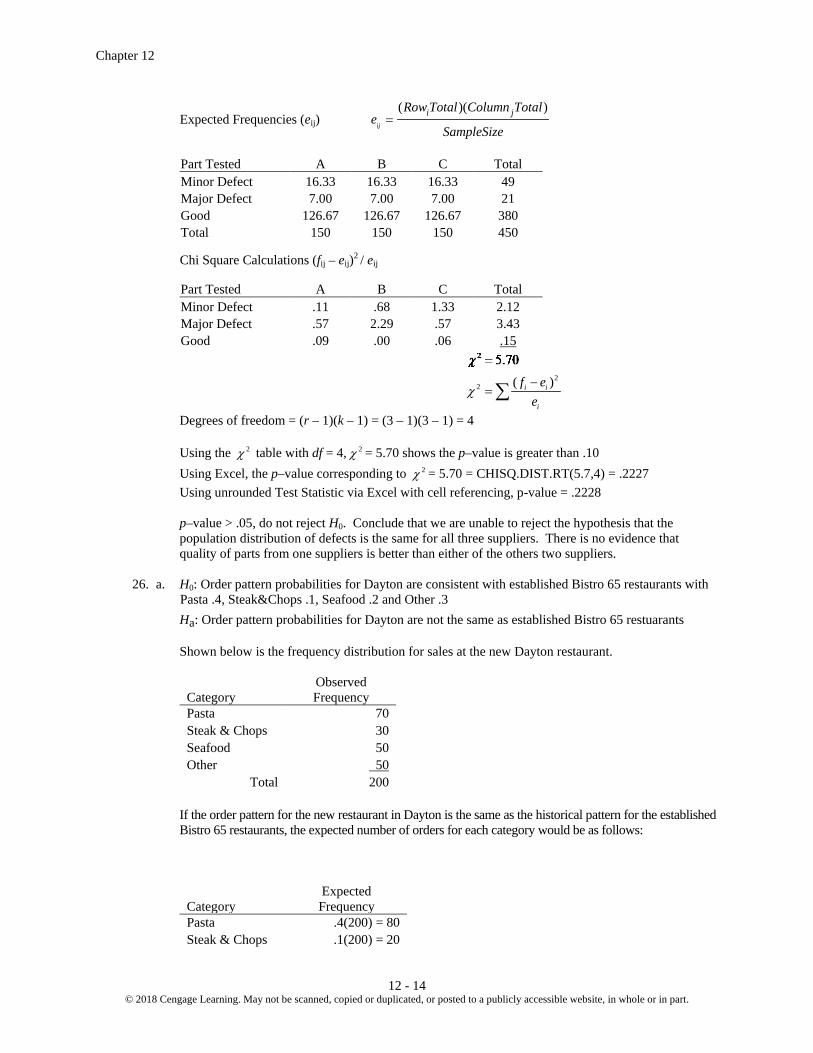
Chapter 12
12 - 14 © 2018 Cengage Learning. May not be scanned, copied or duplicated, or posted to a publicly accessible website, in whole or in part.
Expected Frequencies (eij) ( )( )
ij
i jRow Total Column Totale
SampleSize=
Part Tested A B C Total Minor Defect 16.33 16.33 16.33 49 Major Defect 7.00 7.00 7.00 21 Good 126.67 126.67 126.67 380 Total 150 150 150 450
Chi Square Calculations (fij – eij)2 / eij
Part Tested A B C Total Minor Defect .11 .68 1.33 2.12 Major Defect .57 2.29 .57 3.43 Good .09 .00 .06 .15
2
2 ( )i i
i
f ee
χ−
= ∑
Degrees of freedom = (r – 1)(k – 1) = (3 – 1)(3 – 1) = 4 Using the 2χ table with df = 4, 2χ = 5.70 shows the p–value is greater than .10 Using Excel, the p–value corresponding to 2χ = 5.70 = CHISQ.DIST.RT(5.7,4) = .2227 Using unrounded Test Statistic via Excel with cell referencing, p-value = .2228
p–value > .05, do not reject H0. Conclude that we are unable to reject the hypothesis that the population distribution of defects is the same for all three suppliers. There is no evidence that quality of parts from one suppliers is better than either of the others two suppliers.
26. a. H0: Order pattern probabilities for Dayton are consistent with established Bistro 65 restaurants with Pasta .4, Steak&Chops .1, Seafood .2 and Other .3
Ha: Order pattern probabilities for Dayton are not the same as established Bistro 65 restuarants Shown below is the frequency distribution for sales at the new Dayton restaurant.
Category
Observed Frequency
Pasta 70 Steak & Chops 30 Seafood 50 Other 50
Total 200 If the order pattern for the new restaurant in Dayton is the same as the historical pattern for the established
Bistro 65 restaurants, the expected number of orders for each category would be as follows:
Category
Expected Frequency
Pasta .4(200) = 80 Steak & Chops .1(200) = 20

Tests of Goodness of Fit and Independence
12 - 15 © 2018 Cengage Learning. May not be scanned, copied or duplicated, or posted to a publicly accessible website, in whole or in part.
Seafood .2(200) = 40 Other .3(200) = 60
Total 200
Observed Expected Hypothesized Frequency Frequency Chi Square
Category Proportion (p) (fi) (ei) = n*p (fi – ei)2 / ei Bank .4 70 80 1.25 Cable .1 30 20 5.00 Car .2 50 40 2.50
Collection .3 50 60 1.67 Total: 200 = n 2χ = 10.42
2
2 ( )i i
i
f ee
χ−
= ∑
k – 1 = 4 – 1 = 3 degrees of freedom Using the 2χ table with df = 3, 2χ = 10.42 shows the p–value is between .01 and .025 Using Excel, the p–value corresponding to 2χ = 10.42; = CHISQ.DIST.RT(10.42,3) = .0153 p–value <.05, reject H0. We reject the hypothesis that the order pattern for Dayton is the same as the
order pattern of established Bistro 65 restaurants. Similarly, using Excel’s CHISQ.TEST function with the above observed and expected frequencies
the p-value associated with the chi-square test for goodness of fit is .0153.Because thep-value =.0153 <α = .05, we reject the hypothesis the order pattern for the new restaurant in Dayton is the same as the order pattern for the established Bistro 65 restaurants.
b. The side-by-side bar chart below compares the purchase preference probabilities for the new restaurant in
Dayton and the established or “old” Bistro 65 restaurants. We see that the new restaurant sells a larger percentage of Steak & Chops and Seafood, but a lower percentage of Pasta Other foods.
00.05
0.10.15
0.20.25
0.30.35
0.40.45
Pasta Steak & Chops Seafood Other
Prob
abili
ty
Entree
New
Old

Chapter 12
12 - 16 © 2018 Cengage Learning. May not be scanned, copied or duplicated, or posted to a publicly accessible website, in whole or in part.
28. a. H0:The preferred pace of life is independent of gender Ha:The preferred pace of life is not independent of gender Observed Frequency (fij)
Preferred Gender Pace of Life Male Female Total
Slower 230 218 448 No Preference 20 24 44 Faster 90 48 138 Total 340 290 630
Expected Frequency (eij) ( )( )
ij
i jRow Total Column Totale
SampleSize=
Preferred Gender
Pace of Life Male Female Total Slower 241.78 206.22 448 No Preference 23.75 20.25 44 Faster 74.48 63.52 138 Total 340 290 630
Chi Square Calculations (fij–eij)2/eij
Preferred Gender Pace of Life Male Female Total
Slower .57 .67 1.25 No Preference .59 .69 1.28 Faster 3.24 3.79 7.03
2
2 ( )i i
i
f ee
χ−
= ∑
Degrees of freedom = (r – 1)(c – 1) = (3 – 1)(2 – 1) = 2
Using the 2χ table with df = 2, 2χ = 9.56 shows the p–value is between .005 and .01. Using Excel, the p–value corresponding to 2χ = 9.56= CHISQ.DIST.RT(9.56,2) = .0084.
p–value < .05, reject H0. The preferred pace of life is not independent of gender. Thus, we expect men and women differ with respect to the preferred pace of life.
b. Percentage responses for each gender Column percentages = Gender&Pace Frequency/Gender Total: for example: 230/340 = 67.65%
Preferred Gender Pace of Life Male Female Slower 67.65% 75.17% No Preference 5.88% 8.28% Faster 26.47% 16.55%

Tests of Goodness of Fit and Independence
12 - 17 © 2018 Cengage Learning. May not be scanned, copied or duplicated, or posted to a publicly accessible website, in whole or in part.
The highest percentages are for a slower pace of life by both men and women. However, 75.17% of women prefer a slower pace compared to 67.65% of men and 26.47% of men prefer a faster pace compared to 16.55% of women. More women prefer a slower pace while more men prefer a faster pace.
30. H0:Emergency calls within each county are independent of the day of week Ha: Emergency calls within each county are not independent of the day of week Observed Frequencies (fij)
Day of Week
County Sun Mon Tues Wed Thu Fri Sat Total Urban 61 48 50 55 63 73 43 393 Rural 7 9 16 13 9 14 10 78 Total 68 57 66 68 72 87 53 471
Expected Frequencies (eij) ( )( )
ij
i jRow Total Column Totale
SampleSize=
Day of Week
County Sun Mon Tue Wed Thu Fri Sat Total Urban 56.74 47.56 55.07 56.74 60.08 72.59 44.22 393 Rural 11.26 9.44 10.93 11.26 11.92 14.41 8.78 78 Total 68 57 66 68 72 87 53 471
Chi Square (fij – eij)2/eij
Day of Week
County Sun Mon Tue Wed Thu Fri Sat Total Urban .32 .00 .47 .05 .14 .00 .03 1.02 Rural 1.61 .02 2.35 .27 .72 .01 .17 5.15
2χ = 6.17
2
2 ( )i i
i
f ee
χ−
= ∑
Degrees of freedom =(r – 1)(c – 1) = (2 – 1)(7 – 1) =6 Using the 2χ table with df = 6, 2χ = 6.17 shows the p–value is greater than .10. Using Excel, the p–value corresponding to 2χ = 6.17 = CHISQ.DIST.RT(6.17,6) = .4044. Using unrounded Test Statistic via Excel with cell referencing, p-value = .4039 p–value > .05, do not reject H0. The assumption of independence cannot be rejected. The county
with the emergency call does not vary or depend upon the day of the week.

Chapter 12
12 - 18 © 2018 Cengage Learning. May not be scanned, copied or duplicated, or posted to a publicly accessible website, in whole or in part.
32. a. Bridgeport 8.8%, Los Alamos 11.7%, Naples 9%, Washington DC 8.5% b. H0: 1 2 3 4p p p p= = =
Ha:Not all population proportions are equal Observed Frequencies (fij)
Millionaire Bridgeport Los' Alamos Naples Washington Total Yes 44 35 36 34 149 No 456 265 364 366 1451 Total 500 300 400 400 1600
Expected Frequencies (eij) ( )( )
ij
i jRow Total Column Totale
SampleSize=
Millionaire Bridgeport Los' Alamos Naples Washington Total Yes 46.56 27.94 37.25 37.25 149 No 453.44 272.06 362.75 362.75 1451 Total 500 300 400 400 1600
Chi Square Calculations (fij – eij)2 / eij
Millionaire Bridgeport Los' Alamos Naples Washington Total Yes .14 1.79 .04 .28 2.25 No .01 .18 .00 .03 .23
22 ( )i i
i
f ee
χ−
= ∑
Degrees of freedom = k – 1 = (4 – 1) = 3 Using the 2χ table with df = 3, 2χ = 2.48 shows the p–value is greater than .10 Using Excel, the p–value corresponding to 2χ = 2.48 = CHISQ.DIST.RT(2.48,3) = .4789 Using unrounded Test Statistic via Excel with cell referencing, p-value = .4783
p–value > .05, do not reject H0. Cannot conclude that there is a difference among the population proportion of millionaires for these four cities.

Experimental Design and Analysis of Variance
13 - 1 © 2018 Cengage Learning. May not be scanned, copied or duplicated, or posted to a publicly accessible website, in whole or in part.
Chapter 13 Experimental Design and Analysis of Variance Solutions: 1. a. x = (156 + 142 + 134)/3 = 144 Note: When the sample sizes are the same, the overall sample
mean is an average of the individual sample means.
2
1SSTR
k
j jj
n x x
= 6(156 - 144) 2 + 6(142 - 144) 2 + 6(134 - 144) 2 = 1,488
b. MSTR = SSTR /(k - 1) = 1488/2 = 744 c. 2
1s = 164.4 22s = 131.2 2
3s = 110.4
2
1SSE ( 1)
k
j jj
n s
= 5(164.4) + 5(131.2) +5(110.4) = 2030
d. MSE = SSE /(nT - k) = 2030/(18 - 3) = 135.3 e. Using data in problem, the Excel ANOVA (Single Factor) tool can be used to generate table (Note
that in the Excel generated output, the Between Groups Variation is the Treatments and Within Groups Variation is Error.), or values can be filled in from parts a-d, adding F = MSTR/MSE = 744/135.3 = 5.5
Using Excel, the p-value corresponding to F = 5.5 = F.DIST.RT(5.5,2,15) = .0162 .
Source of Variation
Sum of Squares
Degrees of Freedom
Mean Square
F
p-value
Treatments 1488 2 744 5.50 .0162 Error 2030 15 135.3 Total 3518 17
f. H0: µ1 = µ2 = µ3 Ha: Not all the treatment population means are equal F = MSTR /MSE = 744/135.3 = 5.50 Using F table (2 degrees of freedom numerator and 15 denominator), p-value is between .01 and
.025 Using Excel, the p-value corresponding to F = 5.50 = F.DIST.RT(5.5,2,15) = .0162. Because p-value = .05, we reject the hypothesis that the means for the three treatments are
equal.

Chapter 13
13 - 2 © 2018 Cengage Learning. May not be scanned, copied or duplicated, or posted to a publicly accessible website, in whole or in part.
2. Source of Variation
Sum of Squares
Degrees of Freedom
Mean Square
F
p-value
Treatments 300 4 75 14.07 .0000 Error 160 30 5.33 Total 460 34
SSE = SST - SSTR = 460 – 300 = 160 Treatments degrees of freedom = k-1 = 5-1 = 4, where k = the number of factors/treatments/samples being compared Total observations = nT = 5*7 = 35 Total df = nT-1 = 35-1 = 34 Error df = nT-k = 35 – 5 = 30 MSTR = SSTR/(k-1) = 300/4 = 75 MSE = SSE/(nT-k) = 160/30 = 5.33 F = MSTR/MSE = 75/5.33 = 14.07 Using Excel, the p-value corresponding to F = 14.07 = F.DIST.RT(14.07,4,30) = .0000. 4. H0: µ1 = µ2 = µ3 Ha: Not all the treatment population means are equal
Source of Variation
Sum of Squares
Degrees of Freedom
Mean Square
F
p-value
Treatments 150 2 75 4.80 .0233 Error 250 16 15.625 Total 400 18
SSE = SST – SSTR = 400 – 150 = 250 Treatments degrees of freedom = k-1 = 3-1 = 2, where k = the number of factors/treatments/samples being compared Total observations = nT = 19 Total df = nT-1 = 19-1 = 18 Error df = nT-k = 19 – 3 = 16 MSTR = SSTR/(k-1) = 150/2 = 75 MSE = SSE/(nT-k) = 250/16 = 15.625 F = MSTR/MSE = 75/15.6.25 = 4.8 Using F table (2 degrees of freedom numerator and 16 denominator), p-value is between .01 and
.025 Using Excel, the p-value corresponding to F = 4.80 = F.DIST.RT(4.8,2,16) = .0233. Because p-value = .05, we reject the null hypothesis that the means of the three treatments are
equal.

Experimental Design and Analysis of Variance
13 - 3 © 2018 Cengage Learning. May not be scanned, copied or duplicated, or posted to a publicly accessible website, in whole or in part.
6. H0: µ1 = µ2 = µ3 Ha: Not all the treatment population means are equal Using Exer6 datafile, the Excel Single Factor ANOVA Output follows:
Anova: Single Factor
SUMMARY Groups Count Sum Average Variance
A 8 952 119 146.857 B 10 1070 107 96.4444 C 10 1000 100 173.778
ANOVA Source of Variation SS df MS F P-value
Between Groups 1617.857 2 808.9286 5.8449 0.0083 Within Groups 3460 25 138.4 Total 5077.857 27
Note that Between Groups Variation is the Treatments and Within Groups Variation is Error.
A B C Sample Mean 119 107 100 Sample Variance 146.86 96.44 173.78
1 1 2 2 ... 8(119) 10(107) 10(100) 107.9328
k k
T
n x n x n xx
n
2
1SSTR
k
j jj
n x x
= 8(119 - 107.93) 2 + 10(107 - 107.93) 2 + 10(100 - 107.93) 2 = 1617.86
MSTR = SSTR /(k - 1) = 1617.86 /2 = 808.93
2
1SSE ( 1)
k
j jj
n s
= 7(146.86) + 9(96.44) + 9(173.78) = 3,460
MSE = SSE /(nT - k) = 3,460 /(28 - 3) = 138.4 F = MSTR /MSE = 808.93 /138.4 = 5.84 Using F table (2 degrees of freedom numerator and 25 denominator), p-value is less than .01 Using Excel, the p-value corresponding to F = 5.84 = F.DIST.RT(5.84,2,25) = .0083. Because p-value = .05, we reject the null hypothesis that the means of the three treatments are
equal.

Chapter 13
13 - 4 © 2018 Cengage Learning. May not be scanned, copied or duplicated, or posted to a publicly accessible website, in whole or in part.
8. H0: µ1 = µ2 = µ3 Ha: Not all the treatment population means are equal x = (79 + 74 + 66)/3 = 73Note: When the samplesizes are the same, the overall sample mean is an
average of the individual sample means.
2
1SSTR
k
j jj
n x x
= 6(79 - 73) 2 + 6(74 - 73) 2 + 6(66 - 73) 2 = 516
MSTR = SSTR /(k - 1) = 516/2 = 258 2
1s = 34 22s = 20 2
3s = 32
2
1SSE ( 1)
k
j jj
n s
= 5(34) + 5(20) +5(32) = 430
MSE = SSE /(nT - k) = 430/(18 - 3) = 28.67 F = MSTR /MSE = 258/28.67 = 9.00 Using data in NCP datafile, the Excel ANOVA (Single Factor) tool can be used to generate table
(Note that in the Excel generated output, the Between Groups Variation is the Treatments and Within Groups Variation is Error.), or values can be filled in from calculations above
Source of Variation
Sum of Squares
Degrees of Freedom
Mean Square
F
p-value
Treatments 516 2 258 9.00 .0027 Error 430 15 28.67 Total 946 17
Using F table (2 degrees of freedom numerator and 15 denominator), p-value is less than .01 Using Excel the p-value corresponding to F = 9.00 = F.DIST.RT(9,2,15) = .0027. Because p-value = .05, we reject the null hypothesis that the means for the three plants are
equal. In other words, analysis of variance supports the conclusion that the population mean examination score at the three NCP plants are not equal.
10. H0: µ1 = µ2 = µ3 Ha: Not all the treatment population means are equal Using AudJudg datafile, the Excel Single Factor ANOVA Output follows:
Anova: Single Factor
SUMMARY Groups Count Sum Average Variance
Direct 7 119 17 5.01Indirect 7 142.8 20.4 6.256667Combination 7 175 25 4.01
ANOVA Source of Variation SS df MS F P-value
Between Groups 225.68 2 112.84 22.15928 0.000014

Experimental Design and Analysis of Variance
13 - 5 © 2018 Cengage Learning. May not be scanned, copied or duplicated, or posted to a publicly accessible website, in whole or in part.
Within Groups 91.66 18 5.092222Total 317.34 20
Note that Between Groups Variation is the Treatments and Within Groups Variation is Error.
Direct Experience
Indirect Experience
Combination
Sample Mean 17.0 20.4 25.0 Sample Variance 5.01 6.2567 4.01
x = (17 + 20.4 + 25)/3 = 20.8 Note: When the sample sizes are the same, the overall sample
mean is an average of the individual sample means.
2
1SSTR
k
j jj
n x x
= 7(17 - 20.8) 2 + 7(20.4 - 20.8) 2 + 7(25 - 20.8) 2 = 225.68
MSTR = SSTR /(k - 1) = 225.68 /2 = 112.84
2
1SSE ( 1)
k
j jj
n s
= 6(5.01) + 6(6.2567) + 6(4.01) = 91.66
MSE = SSE /(nT - k) = 91.66 /(21 - 3) = 5.092 F = MSTR /MSE = 112.84 /5.092 = 22.16 Using F table (2 degrees of freedom numerator and 18 denominator), p-value is less than .01 Using Excel the p-value corresponding to F = 22.16 = F.DIST.RT(22.16,2,18) = .0000. Because p-value = .05, we reject the null hypothesis that the means for the three groups are
equal. 12. H0: µ1 = µ2 = µ3 Ha: Not all the treatment population means are equal Using GrandStrand datafile, the Excel Single Factor ANOVA Output follows:
Anova: Single Factor
SUMMARY Groups Count Sum Average Variance
Italian 8 136 17 14.85714 Seafood 8 152 19 13.71429 Steakhouse 8 192 24 14
ANOVA Source of Variation SS df MS F P-value
Between Groups 208 2 104 7.328859 0.003852 Within Groups 298 21 14.19048 Total 506 23
Note that Between Groups Variation is the Treatments and Within Groups Variation is Error.
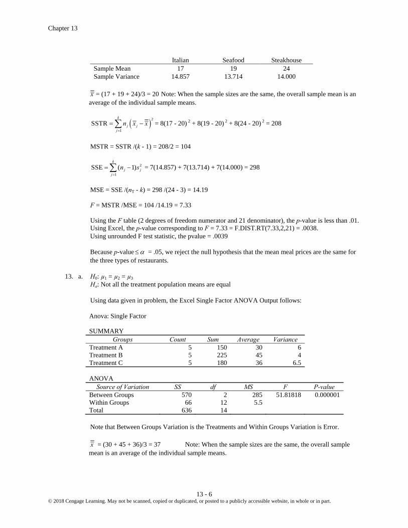
Chapter 13
13 - 6 © 2018 Cengage Learning. May not be scanned, copied or duplicated, or posted to a publicly accessible website, in whole or in part.
Italian Seafood Steakhouse Sample Mean 17 19 24 Sample Variance 14.857 13.714 14.000
x = (17 + 19 + 24)/3 = 20 Note: When the sample sizes are the same, the overall sample mean is an
average of the individual sample means.
2
1SSTR
k
j jj
n x x
= 8(17 - 20) 2 + 8(19 - 20) 2 + 8(24 - 20) 2 = 208
MSTR = SSTR /(k - 1) = 208/2 = 104
2
1SSE ( 1)
k
j jj
n s
= 7(14.857) + 7(13.714) + 7(14.000) = 298
MSE = SSE /(nT - k) = 298 /(24 - 3) = 14.19 F = MSTR /MSE = 104 /14.19 = 7.33 Using the F table (2 degrees of freedom numerator and 21 denominator), the p-value is less than .01. Using Excel, the p-value corresponding to F = 7.33 = F.DIST.RT(7.33,2,21) = .0038. Using unrounded F test statistic, the pvalue = .0039 Because p-value = .05, we reject the null hypothesis that the mean meal prices are the same for
the three types of restaurants. 13. a. H0: µ1 = µ2 = µ3 Ha: Not all the treatment population means are equal Using data given in problem, the Excel Single Factor ANOVA Output follows:
Anova: Single Factor
SUMMARY Groups Count Sum Average Variance
Treatment A 5 150 30 6 Treatment B 5 225 45 4 Treatment C 5 180 36 6.5
ANOVA Source of Variation SS df MS F P-value
Between Groups 570 2 285 51.81818 0.000001 Within Groups 66 12 5.5 Total 636 14
Note that Between Groups Variation is the Treatments and Within Groups Variation is Error. x = (30 + 45 + 36)/3 = 37 Note: When the sample sizes are the same, the overall sample
mean is an average of the individual sample means.

Experimental Design and Analysis of Variance
13 - 7 © 2018 Cengage Learning. May not be scanned, copied or duplicated, or posted to a publicly accessible website, in whole or in part.
2
1SSTR
k
j jj
n x x
= 5(30 - 37)2 + 5(45 - 37)2 + 5(36 - 37)2 = 570
MSTR = SSTR /(k - 1) = 570/2 = 285
2
1SSE ( 1)
k
j jj
n s
= 4(6) + 4(4) + 4(6.5) = 66
MSE = SSE /(nT - k) = 66/(15 - 3) = 5.5 F = MSTR /MSE = 285/5.5 = 51.82 Using F table (2 degrees of freedom numerator and 12 denominator), p-value is less than .01 Using Excel, the p-value corresponding to F = 51.82 = F.DIST.RT(51.82,2,12) = .0000. Because p-value = .05, we reject the null hypothesis that the means of the three populations are
equal. b. t.025 for 12 df = 2.179
/ 2 .0251 1 1 1LSD MSE 5.5 2.179 2.2 3.23
5 5i j
t tn n
1 2 30 45 15x x LSD; significant difference 1 3 30 36 6x x LSD; significant difference 2 3 45 36 9x x LSD; significant difference
c. 1 2 / 21 2
1 1MSEx x tn n
1 1(30 45) 2.179 5.55 5
-15 3.23 = -18.23 to -11.77 14. a. H0: µ1 = µ2 = µ3 Ha: Not all the treatment population means are equal Using data given in problem, the Excel Single Factor ANOVA Output follows:
Anova: Single Factor
SUMMARY Groups Count Sum Average Variance
Treatment 1 4 204 51 96.66667 Treatment 2 4 308 77 97.33333 Treatment 3 4 232 58 82
ANOVA

Chapter 13
13 - 8 © 2018 Cengage Learning. May not be scanned, copied or duplicated, or posted to a publicly accessible website, in whole or in part.
Source of Variation SS df MS F P-value Between Groups 1448 2 724 7.869565 0.010565 Within Groups 828 9 92 Total 2276 11
Note that Between Groups Variation is the Treatments and Within Groups Variation is Error.
Sample 1 Sample 2 Sample 3 Sample Mean 51 77 58 Sample Variance 96.67 97.34 81.99
x = (51 + 77 + 58)/3 = 62 Note: When the sample sizes are the same, the overall sample mean is an
average of the individual sample means.
2
1SSTR
k
j jj
n x x
= 4(51 - 62) 2 +4(77 - 62) 2 + 4(58 - 62) 2 = 1,448
MSTR = SSTR /(k - 1) = 1,448/2 = 724
2
1SSE ( 1)
k
j jj
n s
= 3(96.67) + 3(97.34) + 3(81.99) = 828
MSE = SSE /(nT - k) = 828/(12 - 3) = 92 F = MSTR /MSE = 724/92 = 7.87 Using F table (2 degrees of freedom numerator and 9 denominator), p-value is between .01 and .025 Using Excel, the p-value corresponding to F = 7.87 = F.DIST.RT(7.87,2,9) = .0106 Because p-value = .05, we reject the null hypothesis that the means of the three populations are
equal. b. t.025 for 9 df = 2.262
/ 2 .0251 1 1 1LSD MSE 92 2.262 46 15.34
4 4i j
t tn n
1 2 51 77 26x x LSD; significant difference 1 3 51 58 7x x LSD; no significant difference 2 3 77 58 19x x LSD; significant difference 15. a. H0: µ1 = µ2 = µ3 Ha: Not all the treatment population means are equal Using data given in problem, the Excel Single Factor ANOVA Output follows:

Experimental Design and Analysis of Variance
13 - 9 © 2018 Cengage Learning. May not be scanned, copied or duplicated, or posted to a publicly accessible website, in whole or in part.
Anova: Single Factor
SUMMARY Groups Count Sum Average Variance
Mfg 1 4 92 23 6.666667 Mfg 2 4 112 28 4.666667 Mfg 3 4 84 21 3.333333 ANOVA
Source of Variation SS df MS F P-value Between Groups 104 2 52 10.63636 0.00426 Within Groups 44 9 4.888889 Total 148 11
Note that Between Groups Variation is the Treatments and Within Groups Variation is Error.
Manufacturer 1 Manufacturer 2 Manufacturer 3 Sample Mean 23 28 21 Sample Variance 6.667 4.667 3.333
x = (23 + 28 + 21)/3 = 24 Note: When the sample sizes are the same, the overall sample
mean is an average of the individual sample means.
2
1SSTR
k
j jj
n x x
= 4(23 - 24) 2 + 4(28 - 24) 2 + 4(21 - 24) 2 = 104
MSTR = SSTR /(k - 1) = 104/2 = 52
2
1SSE ( 1)
k
j jj
n s
= 3(6.667) + 3(4.667) + 3(3.33) = 44
MSE = SSE /(nT - k) = 44/(12 - 3) = 4.889 F = MSTR /MSE = 52/4.889 = 10.636 Using F table (2 degrees of freedom numerator and 9 denominator), p-value is less than .01 Using Excel, the p-value corresponding to F = 10.636= F.DIST.RT(10.636,2,9) = .0043 Because p-value = .05, we reject the null hypothesis that the mean time needed to mix a batch
of material is the same for each manufacturer. b. t.025 for 9 df = 2.262
/2 .0251 3
1 1 1 1LSD MSE 4.889 2.262 2.445 3.544 4
t tn n
Since 1 3 23 21 2 3.54,x x there does not appear to be any significant difference between
the means for manufacturer 1 and manufacturer 3.
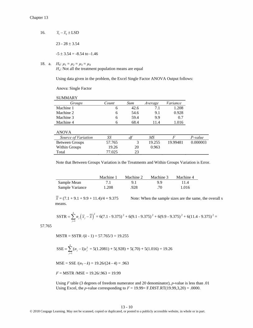
Chapter 13
13 - 10 © 2018 Cengage Learning. May not be scanned, copied or duplicated, or posted to a publicly accessible website, in whole or in part.
16. 1 2 LSDx x 23 - 28 3.54 -5 3.54 = -8.54 to -1.46 18. a. H0: µ1 = µ2 = µ3 = µ4 Ha: Not all the treatment population means are equal Using data given in the problem, the Excel Single Factor ANOVA Output follows:
Anova: Single Factor
SUMMARY Groups Count Sum Average Variance
Machine 1 6 42.6 7.1 1.208 Machine 2 6 54.6 9.1 0.928 Machine 3 6 59.4 9.9 0.7 Machine 4 6 68.4 11.4 1.016
ANOVA Source of Variation SS df MS F P-value
Between Groups 57.765 3 19.255 19.99481 0.000003 Within Groups 19.26 20 0.963 Total 77.025 23
Note that Between Groups Variation is the Treatments and Within Groups Variation is Error.
Machine 1 Machine 2 Machine 3 Machine 4 Sample Mean 7.1 9.1 9.9 11.4 Sample Variance 1.208 .928 .70 1.016
x = (7.1 + 9.1 + 9.9 + 11.4)/4 = 9.375 Note: When the sample sizes are the same, the overall s
means.
2
1SSTR
k
j jj
n x x
= 6(7.1 - 9.375) 2 + 6(9.1 - 9.375) 2 + 6(9.9 - 9.375) 2 + 6(11.4 - 9.375) 2 =
57.765 MSTR = SSTR /(k - 1) = 57.765/3 = 19.255
2
1SSE ( 1)
k
j jj
n s
= 5(1.2081) + 5(.928) + 5(.70) + 5(1.016) = 19.26
MSE = SSE /(nT - k) = 19.26/(24 - 4) = .963 F = MSTR /MSE = 19.26/.963 = 19.99 Using F table (3 degrees of freedom numerator and 20 denominator), p-value is less than .01 Using Excel, the p-value corresponding to F = 19.99= F.DIST.RT(19.99,3,20) = .0000.

Experimental Design and Analysis of Variance
13 - 11 © 2018 Cengage Learning. May not be scanned, copied or duplicated, or posted to a publicly accessible website, in whole or in part.
Because p-value = .05, we reject the null hypothesis that the mean time between breakdowns is
the same for the four machines. b. t.025 for 20 df = 2.086
/21 1 1 1LSD MSE 2.086 0.963 2.086 .321 1.18
6 6i j
tn n
2 4 9.1 11.4 2.3x x LSD; significant difference 20. a. H0: µ1 = µ2 = µ3 Ha: Not all the treatment population means are equal To use Excel’s Single Factor ANOVA Tool we must first create three columns for the attendance
data; one column for the attendance data for the North division, one column for the attendance data for the South division, and one column for the attendance data for the West division and then using datafile Triple-A, copy the attendance figures from the various teams into the appropriate columns. Once this is done, Excel’s Single Factor ANOVA Tool can be used to test for any significant difference in the mean attendance for the three divisions.
The Excel Single Factor ANOVA output is shown below:
SUMMARY Groups Count Sum Average Variance
North 646213 7702.167 1692873.8 South 422262 5565.5 1625453.7 West 433719 8429.75 324862.92 ANOVA Source of Variation SS df MS F P-value
Between Groups 18109727 2 9054863 6.9578 0.0111Within Groups 14315319 11 1301393Total 32425405 13
Note that Between Groups Variation is the Treatments and Within Groups Variation is Error.
Because p-value = .0111 = .05, we reject the null hypothesis that the mean attendance values are equal.
b. n1 = 6 n2 = 4 n3 = 4 t/2 is based upon 11 degrees of freedom = 2.201 Comparing North and South
.0251 1 1 1LSD MSE 2.201 1,301,393 1620.76
6 4i j
tn n
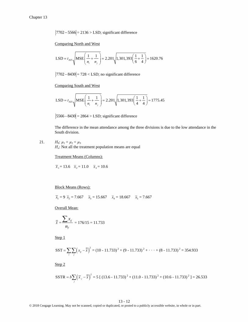
Chapter 13
13 - 12 © 2018 Cengage Learning. May not be scanned, copied or duplicated, or posted to a publicly accessible website, in whole or in part.
7702 5566 = 2136 > LSD; significant difference Comparing North and West
.0251 1 1 1LSD MSE 2.201 1,301,393 1620.76
6 4i j
tn n
7702 8430 = 728 < LSD; no significant difference Comparing South and West
.0251 1 1 1LSD MSE 2.201 1,301,393 1775.45
4 4i j
tn n
5566 8430 = 2864 > LSD; significant difference The difference in the mean attendance among the three divisions is due to the low attendance in the
South division. 21. H0: µ1 = µ2 = µ3 Ha: Not all the treatment population means are equal Treatment Means (Columns): 1x = 13.6 2x = 11.0 3x = 10.6 Block Means (Rows): 1x = 9 2x = 7.667 3x = 15.667 4x = 18.667 5x = 7.667 Overall Mean:
x = ij
T
x
n = 176/15 = 11.733
Step 1
2SST ij
i j
x x = (10 - 11.733) 2 + (9 - 11.733) 2 + · · · + (8 - 11.733) 2 = 354.933
Step 2
2SSTR j
j
b x x = 5 [ (13.6 - 11.733) 2 + (11.0 - 11.733) 2 + (10.6 - 11.733) 2 ] = 26.533

Experimental Design and Analysis of Variance
13 - 13 © 2018 Cengage Learning. May not be scanned, copied or duplicated, or posted to a publicly accessible website, in whole or in part.
Step 3
2SSBL i
i
k x x = 3 [ (9 - 11.733) 2 + (7.667 - 11.733) 2 + (15.667 - 11.733) 2 +
(18.667 - 11.733) 2 + (7.667 - 11.733) 2 ] = 312.267 Step 4 SSE = SST - SSTR - SSBL = 354.933 - 26.533 - 312.267 = 16.133 Treatments degrees of freedom = k-1 = 3-1 = 2, where k = the number of factors/treatments/samples being compared Blocks df = b-1 = 5-1 = 4 Error df = (k-1)(b-1) = 2*4 = 8 Total observations = nT = k*b = 3*5 = 15 Total df = nT-1 = 15-1 = 14 MSTR = SSTR/(k-1) = 26.533/2 = 13.267 MSB = SSB/(b-1) = 312.267/4 = 78.067 MSE = SSE/(nT-k) = 16.133/8 = 2.017 F = MSTR/MSE = 13.267/2.017 = 6.58 Using data given in the problem, the Excel ANOVA (Two-Factor Without Replication) tool can be
used to generate table (Note that in the Excel generated output, the Rows Variation is the Blocks and Columns Variation is Treatments.), or values can be filled in from calculations above
Source of Variation
Sum of Squares
Degrees of Freedom
Mean Square
F
p-value
Treatments 26.5333 2 13.2667 6.58 .0204 Blocks 312.2667 4 78.0667 Error 16.1333 8 2.0167 Total 354.9333 14
Using F table (2 degrees of freedom numerator and 8 denominator), p-value is between .01 and .025 Using Excel, the p-value corresponding to F = 6.58 = F.DIST.RT(6.58,2,8) = .0204. Because p-value = .05, we reject the null hypothesis that the means of the three treatments are
equal. 22. Treatments = k = 5; Blocks = b = 3 H0: µ1 = µ2 = µ3 = µ4 = µ5 Ha: Not all the treatment population means are equal
Source of Variation
Sum of Squares
Degrees of Freedom
Mean Square
F
p-value
Treatments 310 4 77.5 17.71 .0005 Blocks 85 2 42.5 Error 35 8 4.375 Total 430 14

Chapter 13
13 - 14 © 2018 Cengage Learning. May not be scanned, copied or duplicated, or posted to a publicly accessible website, in whole or in part.
SSE = SST – SSTR - SSB = 430 – 310 - 85 = 35 Treatments degrees of freedom = k-1 = 5-1 = 4, where k = the number of factors/treatments/samples being compared Blocks df = b-1 = 3-1 = 2 Error df = (k-1)(b-1) = 4*2 = 8 Total observations = nT = k*b = 3*5 = 15 Total df = nT-1 = 15-1 = 14 MSTR = SSTR/(k-1) = 310/4 = 77.5 MSB = SSB/(b-1) = 85/2 = 42.5 MSE = SSE/(nT-k) = 35/8 = 4.375 F = MSTR/MSE = 77.5/4.375 = 17.71 Using F table (4 degrees of freedom numerator and 8 denominator), p-value is less than .01 Using Excel, the p-value corresponding to F = 17.71 = F.DIST.RT(17.71,4,8) =.0005. Because p-value = .05, we reject the null hypothesis that the means of the treatments are equal. 24. H0: µ1 = µ2 Ha: Not all the treatment population means are equal Treatment Means (Columns): 1x = 56 2x = 44 Block Means (Rows): 1x = 46 2x = 49.5 3x = 54.5 Overall Mean:
x = ij
T
x
n = 300/6 = 50
Step 1
2SST ij
i j
x x = (50 - 50)2 + (42- 50)2 + (55- 50)2+ (44- 50)2 + (63 - 50)2+ (46 - 50)2 = 310
Step 2
2SSTR j
j
b x x = 3 [ (56 - 50) 2 + (44 - 50) 2 ] = 216
Step 3
2SSBL i
i
k x x = 2 [ (46 - 50) 2 + (49.5 - 50) 2 + (54.5 - 50) 2 ] = 73
Step 4 SSE = SST - SSTR - SSBL = 310 - 216 - 73 = 21
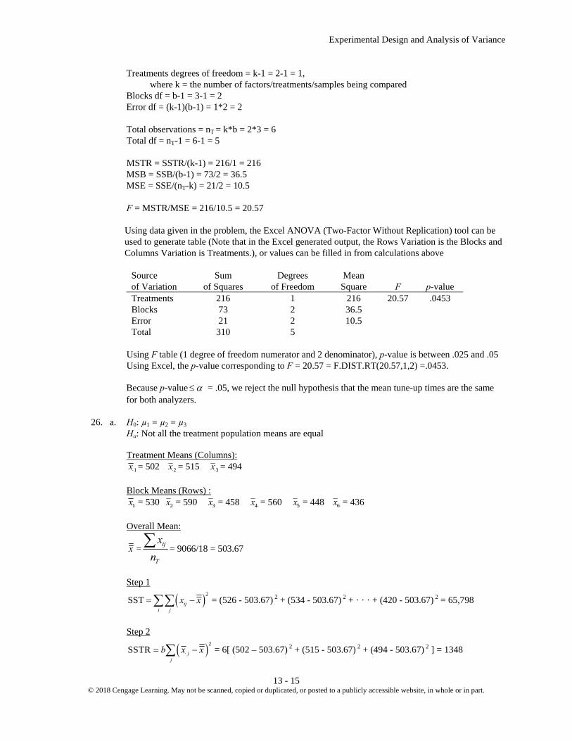
Experimental Design and Analysis of Variance
13 - 15 © 2018 Cengage Learning. May not be scanned, copied or duplicated, or posted to a publicly accessible website, in whole or in part.
Treatments degrees of freedom = k-1 = 2-1 = 1, where k = the number of factors/treatments/samples being compared Blocks df = b-1 = 3-1 = 2 Error df = (k-1)(b-1) = 1*2 = 2 Total observations = nT = k*b = 2*3 = 6 Total df = nT-1 = 6-1 = 5 MSTR = SSTR/(k-1) = 216/1 = 216 MSB = SSB/(b-1) = 73/2 = 36.5 MSE = SSE/(nT-k) = 21/2 = 10.5 F = MSTR/MSE = 216/10.5 = 20.57 Using data given in the problem, the Excel ANOVA (Two-Factor Without Replication) tool can be
used to generate table (Note that in the Excel generated output, the Rows Variation is the Blocks and Columns Variation is Treatments.), or values can be filled in from calculations above
Source of Variation
Sum of Squares
Degrees of Freedom
Mean Square
F
p-value
Treatments 216 1 216 20.57 .0453 Blocks 73 2 36.5 Error 21 2 10.5 Total 310 5
Using F table (1 degree of freedom numerator and 2 denominator), p-value is between .025 and .05 Using Excel, the p-value corresponding to F = 20.57 = F.DIST.RT(20.57,1,2) =.0453. Because p-value = .05, we reject the null hypothesis that the mean tune-up times are the same
for both analyzers. 26. a. H0: µ1 = µ2 = µ3 Ha: Not all the treatment population means are equal
Treatment Means (Columns): 1x = 502 2x = 515 3x = 494 Block Means (Rows) : 1x = 530 2x = 590 3x = 458 4x = 560 5x = 448 6x = 436 Overall Mean:
x = ij
T
x
n = 9066/18 = 503.67
Step 1
2SST ij
i j
x x = (526 - 503.67) 2 + (534 - 503.67) 2 + · · · + (420 - 503.67) 2 = 65,798
Step 2
2SSTR j
j
b x x = 6[ (502 – 503.67) 2 + (515 - 503.67) 2 + (494 - 503.67) 2 ] = 1348

Chapter 13
13 - 16 © 2018 Cengage Learning. May not be scanned, copied or duplicated, or posted to a publicly accessible website, in whole or in part.
Step 3
2SSBL i
i
k x x = 3 [ (530 – 503.67) 2 + (590 - 503.67) 2 + · · · + (436 - 503.67) 2 ] = 63,250
Step 4 SSE = SST - SSTR - SSBL = 65,798- 1348- 63,250= 1200 Treatments degrees of freedom = k-1 = 3-1 = 2, where k = the number of factors/treatments/samples being compared Blocks df = b-1 = 6-1 = 5 Error df = (k-1)(b-1) = 2*5 = 10 Total observations = nT = k*b = 3*6 = 18 Total df = nT-1 = 18-1 = 17 MSTR = SSTR/(k-1) = 1348/2 = 674 MSB = SSB/(b-1) = 63250/5 = 12650 MSE = SSE/(nT-k) = 1200/10 = 120 F = MSTR/MSE = 674/120 = 5.62 Using SATScores datafile, the Excel ANOVA (Two-Factor Without Replication) tool can be used to
generate table (Note that in the Excel generated output, the Rows Variation is the Blocks and Columns Variation is Treatments.), or values can be filled in from calculations above
Source of Variation
Sum of Squares
Degrees of Freedom
Mean Square
F
p-value
Treatments 1348 2 674 5.62 .0231 Blocks 63,250 5 12,650 Error 1200 10 120 Total 65,798 17
Using F table (2 degrees of freedom numerator and 10 denominator), p-value is between .01 and
.025. Using Excel, the p-value corresponding to F = 5.62 = F.DIST.RT(5.62,2,10) = .0231. Using unrounded F test statistic, the pvalue = .0232 Because p-value = .05, we reject the null hypothesis that the mean scores for the three parts of
the SAT are equal. b. The mean test scores for the three sections are 502 for critical reading; 515 for mathematics; and 494
for writing. Because the writing section has the lowest average score, this section appears to give the students the most trouble.
28. H0: Factor means are the same; no interaction effect Ha: Not all factor population means are equal or there is an interaction effect a = number of levels of factor A = 2 b = number of levels of Factor B = 3 r = number of replications = 2 We start by calculating the sample means of each combination of Factor A and Factor B, as well as
overall Factor A means and Factor B means:

Experimental Design and Analysis of Variance
13 - 17 © 2018 Cengage Learning. May not be scanned, copied or duplicated, or posted to a publicly accessible website, in whole or in part.
Factor A
Level 2
Factor B Means
11x = 150
Level 1 Level 2 Level 3 Means
Factor B Factor A
Level 1 12x = 78 13x = 84 1x = 104
21x = 110
1x = 130
22x = 116
2x = 97
23x = 128
3x = 106
2x = 118
x = 111
Step 1
2SST ijk
i j k
x x = (135 - 111) 2 + (165 - 111) 2 + · · · + (136 - 111) 2 = 9,028
Step 2
2SSA i
i
br x x = 3 (2) [ (104 - 111) 2 + (118 - 111) 2 ] = 588
Step 3
2SSB j
j
ar x x = 2 (2) [ (130 - 111) 2 + (97 - 111) 2 + (106 - 111) 2 ] = 2,328
Step 4
2SSAB ij i j
i j
r x x x x = 2 [ (150 - 104 - 130 + 111) 2 + (78 - 104 - 97 + 111) 2 +
· · · + (128 - 118 - 106 + 111) 2 ] = 4,392 Step 5 SSE = SST - SSA - SSB - SSAB = 9,028 - 588 - 2,328 - 4,392 = 1,720 Factor A degrees of freedom = a-1 = 2-1 = 1
Factor B df = b-1 = 3-1 = 2 Interaction df = (a-1)(b-1) = 1*2 = 2
Error df = ab(r-1) = 2*3*1 = 6 Total observations = nT = a*b*r = 2*3*2 = 12 Total df = nT-1 = 12-1 = 11 MSA = SSA/(a-1) = 588/1 = 588 MSB = SSB/(b-1) = 2328/2 = 1164 MSAB = SSAB/[(a-1)(b-1)] = 4392/2 = 2196 MSE = SSE/[ab(r-1)] = 1720/6 = 286.67 FA = MSA/MSE = 588/286.67 = 2.05 FB = MSB/MSE = 1164/286.67 = 4.06 FAB = MSAB/MSE = 2196/286.67 = 7.66

Chapter 13
13 - 18 © 2018 Cengage Learning. May not be scanned, copied or duplicated, or posted to a publicly accessible website, in whole or in part.
Using data given in the problem, the Excel ANOVA (Two-Factor With Replication) tool can be used to generate table (Note that in the Excel generated output, the Sample Variation is Factor A, Columns Variation is Factor B, and Within is Error.), or values can be filled in from calculations above
Source of Variation
Sum of Squares
Degrees of Freedom
Mean Square
F
p-value
Factor A 588 1 588 2.05 .2022 Factor B 2328 2 1164 4.06 .0767 Interaction 4392 2 2196 7.66 .0223 Error 1720 6 286.67 Total 9028 11
Factor A: F = 2.05 Using F table (1 degree of freedom numerator and 6 denominator), p-value is greater than .10 Using Excel, the p-value corresponding to F = 2.05= F.DIST.RT(2.05,1,6) = .2022. Using unrounded F test statistic, the pvalue = .2021 Because p-value > = .05, Factor A is not significant Factor B: F = 4.06 Using F table (2 degrees of freedom numerator and 6 denominator), p-value is between .05 and .10 Using Excel, the p-value corresponding to F = 4.06 = F.DIST.RT(4.06,2,6) = .0767. Because p-value > = .05, Factor B is not significant Interaction: F = 7.66 Using F table (2 degrees of freedom numerator and 6 denominator), p-value is between .01 and .025 Using Excel, the p-value corresponding to F = 7.66 = F.DIST.RT(7.66,2,6) =.0223. Because p-value = .05, Interaction is significant 30. H0: Factor means are the same; no interaction effect Ha: Not all factor population means are equal or there is an interaction effect a = number of levels of factor A = 3 b = number of levels of Factor B = 2 r = number of replications = 2 We start by calculating the sample means of each combination of Factor A and Factor B, as well as
overall Factor A means and Factor B means: Factor A is advertising design; Factor B is size of advertisement.

Experimental Design and Analysis of Variance
13 - 19 © 2018 Cengage Learning. May not be scanned, copied or duplicated, or posted to a publicly accessible website, in whole or in part.
Factor A B
Factor B Means
11x = 10
Small Large Means
Factor B Factor A
12x = 10 1x = 10
21x = 18
1x = 14
22x = 28
2x = 18
2x = 23
x = 16
A
C 31x = 14 32x = 16 3x = 15
Step 1
2SST ijk
i j k
x x = (8 - 16) 2 + (12 - 16) 2 + (12 - 16) 2 + · · · + (14 - 16) 2 = 544
Step 2
2SSA i
i
br x x = 2 (2) [ (10- 16) 2 + (23 - 16) 2 + (15 - 16) 2 ] = 344
Step 3
2SSB j
j
ar x x = 3 (2) [ (14 - 16) 2 + (18 - 16) 2 ] = 48
Step 4
2SSAB ij i j
i j
r x x x x = 2 [ (10 - 10 - 14 + 16) 2 + · · · + (16 - 15 - 18 +16) 2 ] = 56
Step 5 SSE = SST - SSA - SSB - SSAB = 544 - 344 - 48 - 56 = 96 Factor A degrees of freedom = a-1 = 3-1 = 2
Factor B df = b-1 = 2-1 = 1 Interaction df = (a-1)(b-1) = 2*1 = 2
Error df = ab(r-1) = 3*2*1 = 6 Total observations = nT = a*b*r = 3*2*2 = 12 Total df = nT-1 = 12-1 = 11 MSA = SSA/(a-1) = 344/2 = 172 MSB = SSB/(b-1) = 48/1 = 48 MSAB = SSAB/[(a-1)(b-1)] = 56/2 = 28 MSE = SSE/[ab(r-1)] = 96/6 = 16 FA = MSA/MSE = 172/16 = 10.75 FB = MSB/MSE = 48/16 = 3.00

Chapter 13
13 - 20 © 2018 Cengage Learning. May not be scanned, copied or duplicated, or posted to a publicly accessible website, in whole or in part.
FAB = MSAB/MSE = 28/16 = 1.75 Using data given in the problem, the Excel ANOVA (Two-Factor With Replication) tool can be used
to generate table (Note that in the Excel generated output, the Sample Variation is Factor A, Columns Variation is Factor B, and Within is Error.), or values can be filled in from calculations above
Source of Variation
Sum of Squares
Degrees of Freedom
Mean Square
F
p-value
Factor A 344 2 172 10.75 .0104 Factor B 48 1 48 3.00 .1340 Interaction 56 2 28 1.75 .2519 Error 96 6 16 Total 544 11
Factor A: F = 10.75 Using F table for Factor A (2 degrees of freedom numerator and 6 denominator), p-value is between
.01 and .025 Using Excel, the p-value corresponding to F = 10.75 = F.DIST.RT(10.75,2,6) =.0104. Because p-value = .05, Factor A is significant; there is a difference due to the type of
advertisement design. Factor B: F = 3.00 Using F table for Factor B (1 degree of freedom numerator and 6 denominator), p-value is greater
than .10 Using Excel, the p-value corresponding to F =3.00 = F.DIST.RT(3,1,6) =.1340. Because p-value > = .05, Factor B is not significant; there is not a significant difference due to
size of advertisement. Interaction: F = 1.75 Using F table for Interaction (2 degrees of freedom numerator and 6 denominator), p-value is greater
than .10 Using Excel, the p-value corresponding to F = 1.75 = F.DIST.RT(1.75,2,6) =.2519. Because p-value > = .05, Interaction is not significant. 32. H0: Factor means are the same; no interaction effect Ha: Not all factor population means are equal or there is an interaction effect a = number of levels of factor A = 4 b = number of levels of Factor B = 2 r = number of replications = 2 Using HybridTest datafile with Factor A as Class of vehicle tested (small car, midsize car, small
SUV, and midsize SUV) and Factor B as Type (hybrid or conventional),the data in tabular format is created as follows.
Hybrid ConventionalSmall Car 37 28 44 32

Experimental Design and Analysis of Variance
13 - 21 © 2018 Cengage Learning. May not be scanned, copied or duplicated, or posted to a publicly accessible website, in whole or in part.
Midsize Car 27 23 32 25 Small SUV 27 21 28 22 Midsize SUV 23 19 24 18
Next we calculate the sample means of each combination of Factor A and Factor B, as well as overall Factor A means and Factor B means:
Summary statistics for the above data are shown below:
Hybrid Conventional Small Car 11x = 40.5 12x = 30.0 1x = 35.25
Midsize Car 21x = 29.5 22x = 24.0 2x = 26.75
Small SUV 31x = 27.5 32x = 21.5 3x = 24.50
Midsize SUV 41x = 23.5 42x = 18.5 4x = 21.00
1x = 30.25 2x = 23.5 x = 26.875
Step 1
2SST ijk
i j k
x x = (37 - 26.875) 2 + (44 - 26.875) 2 + · · · + (18 - 26.875) 2 = 691.75
Step 2
2SSA i
i
br x x = 2(2) [(35.25 - 26.875) 2 + (26.75 - 26.875) 2 + (24.5- 26.875) 2
+ (21.0- 26.875) 2] = 441.25 Step 3
2SSB j
j
ar x x = 4(2) [(30.25 - 26.875) 2 + (23.5 - 26.875) 2 ] = 182.25
Step 4
2SSAB ij i j
i j
r x x x x = 2[(40.5- 35.25- 30.25 + 26.875) 2 + (30- 35.25- 23.5+ 26.875) 2
+ · · · + (18.5 – 21.0 – 23.5 + 26.875) 2] = 19.25 Step 5 SSE = SST - SSA - SSB - SSAB = 691.75 – 441.25 – 182.25 – 19.25 = 49 Factor A degrees of freedom = a-1 = 4-1 = 3
Factor B df = b-1 = 2-1 = 1 Interaction df = (a-1)(b-1) = 3*1 = 3
Error df = ab(r-1) = 4*2*1 = 8 Total observations = nT = a*b*r = 4*2*2 = 16 Total df = nT-1 = 16-1 = 15 MSA = SSA/(a-1) = 441.25/3 = 147.083 MSB = SSB/(b-1) = 182.25/1 = 182.25

Chapter 13
13 - 22 © 2018 Cengage Learning. May not be scanned, copied or duplicated, or posted to a publicly accessible website, in whole or in part.
MSAB = SSAB/[(a-1)(b-1)] = 19.25/3 = 6.4167 MSE = SSE/[ab(r-1)] = 49/8 = 6.125 FA = MSA/MSE = 147.083/6.125 = 24.01 FB = MSB/MSE = 182.25/6.125 = 29.76 FAB = MSAB/MSE = 6.4167/6.125 = 1.0476 Using HybridTest datafile, the Excel ANOVA (Two-Factor With Replication) tool can be used to
generate table (Note that in the Excel generated output, the Sample Variation is Factor A, Columns Variation is Factor B, and Within is Error.), or values can be filled in from calculations above
Source of Variation
Sum of Squares
Degrees of Freedom
Mean Square
F
p-
value Factor A 441.25 3 147.083 24.01 .0002 Factor B 182.25 1 182.250 29.76 .0006 Interaction 19.25 3 6.4167 1.0476 .4229 Error 49.00 8 6.125 Total 691.75 15
Factor A: F = 24.01 Using F table for Factor A (3 degree of freedom numerator and 8 denominator), p-value is less than .01
Using Excel, the p-value corresponding to F = 24.01= F.DIST.RT(24.01,3,8) =.0002. Factor A: Because p-value = .0002 <α = .05, Factor A (Class) is significant Factor B: F = 29.76
Using F table for Factor B (1 degrees of freedom numerator and 8 denominator), p-value is less than .01 Using Excel, the p-value corresponding to F = 29.76= F.DIST.RT(29.76,1,8) =.0006. Factor B: Because p-value = .0006 <α = .05, Factor B (Type) is significant Interaction: F = 1.0476
Using F table for Interaction (3 degrees of freedom numerator and 8 denominator), p-value is greater than .10
Using Excel, the p-value corresponding to F = 1.0476= F.DIST.RT(1.0476,3,8) =.4229. Interaction: Because p-value = .4229 >α = .05, Interaction is not significant The class of vehicles has a significant effect on miles per gallon with cars showing more miles per
gallon than SUVs. The type of vehicle also has a significant effect with hybrids having more miles per gallon than conventional vehicles. There is no evidence of a significant interaction effect.
34. H0: µ1 = µ2 = µ3 Ha: Not all the treatment population means are equal Using data given in problem, the Excel Single Factor ANOVA Output follows:

Experimental Design and Analysis of Variance
13 - 23 © 2018 Cengage Learning. May not be scanned, copied or duplicated, or posted to a publicly accessible website, in whole or in part.
Anova: Single Factor
SUMMARY Groups Count Sum Average Variance
x 4 368 92 30 y 4 388 97 6 z 4 336 84 35.33333
ANOVA Source of Variation SS df MS F P-value
Between Groups 344 2 172 7.233645 0.013397 Within Groups 214 9 23.77778 Total 558 11
Note that Between Groups Variation is the Treatments and Within Groups Variation is Error.
X y z Sample Mean 92 97 84 Sample Variance 30 6 35.33
x = (92 + 97 + 84) /3 = 91 Note: When the sample sizes are the same, the overall sample mean is an
average of the individual sample means.
2
1SSTR
k
j jj
n x x
= 4(92 - 91) 2 + 4(97 - 91) 2 + 4(84 - 91) 2 = 344
MSTR = SSTR /(k - 1) = 344 /2 = 172
2
1SSE ( 1)
k
j jj
n s
= 3(30) + 3(6) + 3(35.33) = 214
MSE = SSE /(nT - k) = 214 /(12 - 3) = 23.78 F = MSTR /MSE = 172 /23.78 = 7.23 Using F table (2 degrees of freedom numerator and 9 denominator), p-value is between .01 and .025 Using Excel, the p-value corresponding to F = 7.23 = F.DIST.RT(7.23,2,9) =.0134. Because p-value = .05, we reject the null hypothesis that the mean absorbency ratings for the
three brands are equal. 36. H0: µ1 = µ2 = µ3 = µ4 Ha: Not all the treatment population means are equal Using OzoneLevels datafile, the Excel ANOVA (Two-Factor Without Replication)output is shown
below:
ANOVA Source of Variation SS df MS F P-value F crit
Rows 903.025 9 100.3361 4.5479 0.0010 2.2501 Columns 160.075 3 53.3583 2.4186 0.0880 2.9604

Chapter 13
13 - 24 © 2018 Cengage Learning. May not be scanned, copied or duplicated, or posted to a publicly accessible website, in whole or in part.
Error 595.675 27 22.0620 Total 1658.775 39
The label Rows corresponds to the blocks in the problem (Date), and the label column corresponds
to the treatments (City). Because the p-value corresponding to Columns (treatments) is .0880 >α = .05, there is no significant
difference in the mean ozone level among the four cites. But, if the level of significance was α = .10, the difference would have been significant.
38. H0: µ1 = µ2 = µ3 Ha: Not all the treatment population means are equal Using Assembly datafile, the Excel Single Factor ANOVA Output follows:
Anova: Single Factor
SUMMARY Groups Count Sum Average Variance
A 10 900 90 98 B 10 840 84 168.4444 C 10 810 81 159.7778
ANOVA Source of Variation SS df MS F P-value
Between Groups 420 2 210 1.478102 0.245946 Within Groups 3836 27 142.0741 Total 4256 29
Note that Between Groups Variation is the Treatments and Within Groups Variation is Error.
Method A Method B Method C Sample Mean 90 84 81 Sample Variance 98.00 168.44 159.78
x = (90 + 84 + 81) /3 = 85 Note: When the sample sizes are the same, the overall sample mean is an
average of the individual sample means.
2
1SSTR
k
j jj
n x x
= 10(90 - 85) 2 + 10(84 - 85) 2 + 10(81 - 85) 2 = 420
MSTR = SSTR /(k - 1) = 420 /2 = 210
2
1SSE ( 1)
k
j jj
n s
= 9(98.00) + 9(168.44) + 9(159.78) = 3,836
MSE = SSE /(nT - k) = 3,836 /(30 - 3) = 142.07 F = MSTR /MSE = 210 /142.07 = 1.48
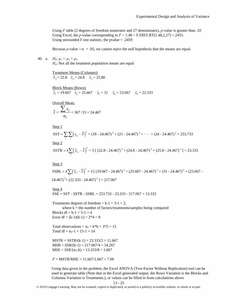
Experimental Design and Analysis of Variance
13 - 25 © 2018 Cengage Learning. May not be scanned, copied or duplicated, or posted to a publicly accessible website, in whole or in part.
Using F table (2 degrees of freedom numerator and 27 denominator), p-value is greater than .10 Using Excel, the p-value corresponding to F = 1.48 = F.DIST.RT(1.48,2,27) =.2455. Using unrounded F test statistic, the pvalue = .2459 Because p-value > = .05, we cannot reject the null hypothesis that the means are equal. 40. a. H0: µ1 = µ2 = µ3 Ha: Not all the treatment population means are equal Treatment Means (Columns): 1x = 22.8 2x = 24.8 3x = 25.80 Block Means (Rows): 1x = 19.667 2x = 25.667 3x = 31 4x = 23.667 5x = 22.333 Overall Mean:
x = ij
T
x
n = 367 /15 = 24.467
Step 1
2SST ij
i j
x x = (18 - 24.467) 2 + (21 - 24.467) 2 + · · · + (24 - 24.467) 2 = 253.733
Step 2
2SSTR j
j
b x x = 5 [ (22.8 - 24.467) 2 + (24.8 - 24.467) 2 + (25.8 - 24.467) 2 ] = 23.333
Step 3
2SSBL i
i
k x x = 3 [ (19.667 - 24.467) 2 + (25.667 - 24.467) 2 + (31 - 24.467) 2 + (23.667 -
24.467) 2+ (22.333 - 24.467) 2 ] = 217.067 Step 4 SSE = SST - SSTR - SSBL = 253.733 - 23.333 - 217.067 = 13.333 Treatments degrees of freedom = k-1 = 3-1 = 2, where k = the number of factors/treatments/samples being compared Blocks df = b-1 = 5-1 = 4 Error df = (k-1)(b-1) = 2*4 = 8 Total observations = nT = k*b = 3*5 = 15 Total df = nT-1 = 15-1 = 14 MSTR = SSTR/(k-1) = 23.333/2 = 11.667 MSB = SSB/(b-1) = 217.067/4 = 54.267 MSE = SSE/(nT-k) = 13.333/8 = 1.667 F = MSTR/MSE = 11.667/1.667 = 7.00 Using data given in the problem, the Excel ANOVA (Two-Factor Without Replication) tool can be
used to generate table (Note that in the Excel generated output, the Rows Variation is the Blocks and Columns Variation is Treatments.), or values can be filled in from calculations above

Chapter 13
13 - 26 © 2018 Cengage Learning. May not be scanned, copied or duplicated, or posted to a publicly accessible website, in whole or in part.
Source of Variation
Sum of Squares
Degrees of Freedom
Mean Square
F
p-value
Treatment 23.333 2 11.667 7.00 .0175 Blocks 217.067 4 54.267 32.56 Error 13.333 8 1.667 Total 253.733 14
Using F table (2 degrees of freedom numerator and 8 denominator), p-value is between .01 and .025 Using Excel, the p-value corresponding to F = 7.00= F.DIST.RT(7,2,8) =.0175. Because p-value = .05, we reject the null hypothesis that the mean miles per gallon ratings for
the three brands of gasoline are equal. b. H0: µ1 = µ2 = µ3 Ha: Not all the treatment population means are equal Completely Randomized Design is Single Factor ANOVA (no blocks) Using data given in the problem, the Excel Single Factor ANOVA Output follows: Anova: Single Factor
Note that Between Groups Variation is the Treatments and Within Groups Variation is Error.
I II III Sample Mean 22.8 24.8 25.8 Sample Variance 21.2 9.2 27.2
x = (22.8 + 24.8 + 25.8) /3 = 24.467 Note: When the sample sizes are the same, the
overall sample mean is an average of the individual sample means.
2
1SSTR
k
j jj
n x x
= 5(22.8 - 24.467) 2 + 5(24.8 - 24.467) 2 + 5(25.8 - 24.467) 2 = 23.333
MSTR = SSTR /(k - 1) = 23.333 /2 = 11.667
2
1SSE ( 1)
k
j jj
n s
= 4(21.2) + 4(9.2) + 4(27.2) = 230.4
SUMMARY Groups Count Sum Average Variance
I 5 114 22.8 21.2 II 5 124 24.8 9.2 III 5 129 25.8 27.2
ANOVA Source of Variation SS df MS F P-value
Between Groups 23.33333 2 11.66667 0.607639 0.56057 Within Groups 230.4 12 19.2 Total 253.7333 14

Experimental Design and Analysis of Variance
13 - 27 © 2018 Cengage Learning. May not be scanned, copied or duplicated, or posted to a publicly accessible website, in whole or in part.
MSE = SSE /(nT - k) = 230.4 /(15 - 3) = 19.2 F = MSTR /MSE = 11.667 /19.2 = .61 Using F table (2 degrees of freedom numerator and 12 denominator), p-value is greater than .10 Using Excel, the p-value corresponding to F = .61 = F.DIST.RT(.61,2,12) =.5594. Using unrounded F test statistic, the pvalue = .5606 Because p-value > = .05, we cannot reject the null hypothesis that the mean miles per gallon
ratings for the three brands of gasoline are equal. Thus, we must remove the block effect in order to detect a significant difference due to the brand of
gasoline. The following table illustrates the relationship between the randomized block design and the completely randomized design.
Sum of Squares
Randomized Block Design
Completely Randomized Design
SST 253.733 253.733 SSTR 23.333 23.333 SSBL 217.067 does not exist SSE 13.333 230.4
Note that SSE for the completely randomized design is the sum of SSBL (217.02) and SSE (13.38)
for the randomized block design. This illustrates that the effect of blocking is to remove the block effect from the error sum of squares; thus, the estimate of for the randomized block design is substantially smaller than it is for the completely randomized design.
42. H0: µ1 = µ2 = µ3 Ha: Not all the treatment population means are equal
Using HoustonAstros datafile, the Excel ANOVA (Two-Factor Without Replication) output is shown below:
ANOVA Source of Variation SS df MS F P-value F crit
Rows 79329936 6 13221656 0.7002 0.6552 2.9961 Columns 1.01E+08 2 50734841 2.6870 0.1086 3.8853 Error 2.27E+08 12 18881427
Total 4.07E+08 20 The label Rows corresponds to the blocks in the problem (Opponent), and the label column
corresponds to the treatments (Day). Because the p-value corresponding to Columns (treatments) is .1086>α = .05, there is no significant
difference in the mean attendance per game for games played on Friday, Saturday, and Sunday. These data do not suggest a particular day on which the Astros should schedule these promotions.
44. H0: Factor means are the same; no interaction effect Ha: Not all factor population means are equal or there is an interaction effect

Chapter 13
13 - 28 © 2018 Cengage Learning. May not be scanned, copied or duplicated, or posted to a publicly accessible website, in whole or in part.
a = number of levels of factor A = 2 b = number of levels of Factor B = 2 r = number of replications = 2 We start by calculating the sample means of each combination of Factor A and Factor B, as well as
overall Factor A means and Factor B means:
Factor A
Machine 2
Factor B Means
11x = 32
Manual Automatic Means
Factor B Factor B
12x = 28 1x = 30
21x = 21
1x = 26.5
22x = 26
2x = 27
2x = 23.5
x = 26.75
Machine 1
Step 1
2SST ijk
i j k
x x = (30 - 26.75) 2 + (34 - 26.75) 2 + · · · + (28 - 26.75) 2 = 151.5
Step 2
2SSA i
i
br x x = 2 (2) [ (30 - 26.75) 2 + (23.5 - 26.75) 2 ] = 84.5
Step 3
2SSB j
j
ar x x = 2 (2) [ (26.5 - 26.75) 2 + (27 - 26.75) 2 ] = 0.5
Step 4
2SSAB ij i j
i j
r x x x x = 2[(32 - 30 - 26.5 + 26.75)2 + · · · + (26 - 23.5 - 27 + 26.75)2]
= 40.5 Step 5 SSE = SST - SSA - SSB - SSAB = 151.5 - 84.5 - 0.5 - 40.5 = 26 Factor A degrees of freedom = a-1 = 2-1 = 1
Factor B df = b-1 = 2-1 = 1 Interaction df = (a-1)(b-1) = 1*1 = 1
Error df = ab(r-1) = 2*2*1 = 4 Total observations = nT = a*b*r = 2*2*2 = 8 Total df = nT-1 = 8-1 = 7 MSA = SSA/(a-1) = 84.5/1 = 84.5 MSB = SSB/(b-1) = .5/1 = .5
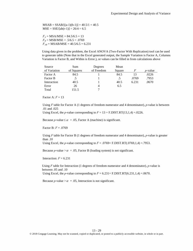
Experimental Design and Analysis of Variance
13 - 29 © 2018 Cengage Learning. May not be scanned, copied or duplicated, or posted to a publicly accessible website, in whole or in part.
MSAB = SSAB/[(a-1)(b-1)] = 40.5/1 = 40.5 MSE = SSE/[ab(r-1)] = 26/4 = 6.5 FA = MSA/MSE = 84.5/6.5 = 13 FB = MSB/MSE = .5/6.5 = .0769 FAB = MSAB/MSE = 40.5/6.5 = 6.231 Using data given in the problem, the Excel ANOVA (Two-Factor With Replication) tool can be used
to generate table (Note that in the Excel generated output, the Sample Variation is Factor A, Columns Variation is Factor B, and Within is Error.), or values can be filled in from calculations above
Source of Variation
Sum of Squares
Degrees of Freedom
Mean Square
F
p-value
Factor A 84.5 1 84.5 13 .0226 Factor B .5 1 .5 .0769 .7953 Interaction 40.5 1 40.5 6.231 .0670 Error 26 4 6.5 Total 151.5 7
Factor A: F = 13 Using F table for Factor A (1 degrees of freedom numerator and 4 denominator), p-value is between
.01 and .025 Using Excel, the p-value corresponding to F = 13 = F.DIST.RT(13,1,4) =.0226. Because p-value = .05, Factor A (machine) is significant. Factor B: F = .0769 Using F table for Factor B (1 degrees of freedom numerator and 4 denominator), p-value is greater
than .10 Using Excel, the p-value corresponding to F = .0769= F.DIST.RT(.0769,1,4) =.7953. Because p-value > = .05, Factor B (loading system) is not significant. Interaction: F = 6.231
Using F table for Interaction (1 degrees of freedom numerator and 4 denominator), p-value is
between .05 and .10 Using Excel, the p-value corresponding to F = 6.231= F.DIST.RT(6.231,1,4) =.0670. Because p-value > = .05, Interaction is not significant.
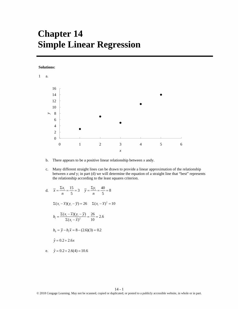
14 - 1 © 2018 Cengage Learning. May not be scanned, copied or duplicated, or posted to a publicly accessible website, in whole or in part.
Chapter 14 Simple Linear Regression Solutions: 1 a.
b. There appears to be a positive linear relationship between x andy. c. Many different straight lines can be drawn to provide a linear approximation of the relationship
between x and y; in part (d) we will determine the equation of a straight line that “best” represents the relationship according to the least squares criterion.
d. 15 403 85 5
i ix yx y
n nΣ Σ
= = = = = =
2( )( ) 26 ( ) 10i i ix x y y x xΣ − − = Σ − =
1 2
( )( ) 26 2.610( )
i i
i
x x y ybx x
Σ − −= = =
Σ −
b y b x0 1 8 2 6 3 0 2= − = − =( . )( ) . ˆ 0.2 2.6y x= + e. ˆ 0.2 2.6(4) 10.6y = + =
02468
10121416
0 1 2 3 4 5 6
y
x

Chapter 14
14 - 2 © 2018 Cengage Learning. May not be scanned, copied or duplicated, or posted to a publicly accessible website, in whole or in part.
2. a.
b. There appears to be a negative linear relationship between x and y. c. Many different straight lines can be drawn to provide a linear approximation of the relationship
between x and y; in part (d) we will determine the equation of a straight line that “best” represents the relationship according to the least squares criterion.
d. 55 17511 355 5
i ix yx y
n nΣ Σ
= = = = = =
2( )( ) 540 ( ) 180i i ix x y y x xΣ − − = − Σ − =
1 2
( )( ) 540 3180( )
i i
i
x x y yb
x xΣ − − −
= = = −Σ −
0 1 35 ( 3)(11) 68b y b x= − = − − = ˆ 68 3y x= −
e. ˆ 68 3(10) 38y = − =
0
10
20
30
40
50
60
0 5 10 15 20 25
y
x

Simple Linear Regression
14 - 3 © 2018 Cengage Learning. May not be scanned, copied or duplicated, or posted to a publicly accessible website, in whole or in part.
4. a.
b. There appears to be a positive linear relationship between the percentage of women working in the
five companies (x) and the percentage of management jobs held by women in that company (y) c. Many different straight lines can be drawn to provide a linear approximation of the relationship
between x and y; in part (d) we will determine the equation of a straight line that “best” represents the relationship according to the least squares criterion.
d. 300 21560 43
5 5i ix yx y
n nΣ Σ
= = = = = =
2( )( ) 624 ( ) 480i i ix x y y x xΣ − − = Σ − =
1 2
( )( ) 624 1.3( ) 480
i i
i
x x y ybx x
Σ − −= = =
Σ −
0 1 43 1.3(60) 35b y b x= − = − = − ˆ 35 1.3y x= − + e. ˆ 35 1.3 35 1.3(60) 43%y x= − + = − + =
0
10
20
30
40
50
60
70
40 45 50 55 60 65 70 75
% M
anag
emen
t
% Working

Chapter 14
14 - 4 © 2018 Cengage Learning. May not be scanned, copied or duplicated, or posted to a publicly accessible website, in whole or in part.
6. a.
b. The scatter diagram indicates a positive linear relationship between x = average number of passing
yards per attempt and y = the percentage of games won by the team. c. / 68 /10 6.8 / 464 /10 46.4i ix x n y y n= Σ = = = Σ = = 2( )( ) 121.6 ( ) 7.08i i ix x y y x xΣ − − = Σ − =
1 2
( )( ) 121.6 17.1751( ) 7.08
i i
i
x x y ybx x
Σ − −= = =
Σ −
0 1 46.4 (17.1751)(6.8) 70.391b y b x= − = − = − ˆ 70.391 17.1751y x= − + d. The slope of the estimated regression line is approximately 17.2. So, for every increase of one yard
in the average number of passes per attempt, the percentage of games won by the team increases by 17.2%.
e. With an average number of passing yards per attempt of 6.2, the predicted percentage of games won
is y = -70.391 + 17.175(6.2) = 36%. With a record of 7 wins and 9 loses, the percentage of wins that the Kansas City Chiefs won is 43.8 or approximately 44%. Considering the small data size, the prediction made using the estimated regression equation is not too bad.
0
10
20
30
40
50
60
70
80
90
4 5 6 7 8 9
Win
%
Yds/Att

Simple Linear Regression
14 - 5 © 2018 Cengage Learning. May not be scanned, copied or duplicated, or posted to a publicly accessible website, in whole or in part.
8. a.
b. The scatter diagram indicates a positive linear relationship between x = speed of executionrating and
y = overall satisfaction rating for electronic trades. c. / 36.3 /11 3.3 / 35.2 /11 3.2i ix x n y y n= Σ = = = Σ = = 2( )( ) 2.36 ( ) 2.6i i ix x y y x xΣ − − = Σ − =
1 2
( )( ) 2.36 .90772.6( )
i i
i
x x y yb
x xΣ − −
= = =Σ −
0 1 3.2 (.9077)(3.3) .2046b y b x= − = − = ˆ .2046 .9077y x= +
d. The slope of the estimated regression line is approximately .9077. So, a one unit increase in the
speed of execution rating will increase the overall satisfaction rating by approximately .9 points.
e. The average speed of execution rating for the other brokerage firms is 3.38. Using this as the new value of x for Zecco.com, we can use the estimated regression equation developed in part (c) to estimate the overall satisfaction rating corresponding to x = 3.38.
ˆ .2046 .9077 .2046 .9077(3.38) 3.27y x= + = + = Thus, an estimate of the overall satisfaction rating when x = 3.38 is approximately 3.3.
2.0
2.5
3.0
3.5
4.0
4.5
2.0 2.5 3.0 3.5 4.0 4.5
Satis
fact
ion
Speed of Execution

Chapter 14
14 - 6 © 2018 Cengage Learning. May not be scanned, copied or duplicated, or posted to a publicly accessible website, in whole or in part.
10. a.
b. The scatter diagram indicates a positive linear relationship between x = age of wineand y = price of a
750 ml bottle of wine. In other words, the price of the wine increases with age. c. / 317 /10 31.7 / 2294 /10 229.4i ix x n y y n= Σ = = = Σ = = 2( )( ) 3838.2 ( ) 552.1i i ix x y y x xΣ − − = Σ − =
1 2
( )( ) 3838.2 6.952( ) 552.1
i i
i
x x y ybx x
Σ − −= = =
Σ −
0 1 229.4 (6.952)(31.7) 9.0216b y b x= − = − = ˆ 9.0216 6.952y x= + d. The slope of the estimated regression line is approximately 6.95. So, for every additional year of age,
the price of the wine increases by $6.95.
0.00
50.00
100.00
150.00
200.00
250.00
300.00
350.00
0 10 20 30 40 50
Pric
e ($
)
Age (years)
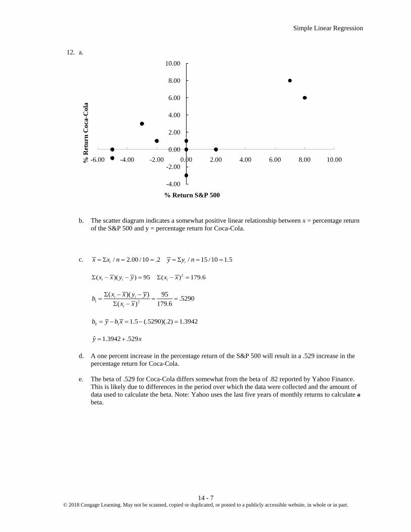
Simple Linear Regression
14 - 7 © 2018 Cengage Learning. May not be scanned, copied or duplicated, or posted to a publicly accessible website, in whole or in part.
12. a.
b. The scatter diagram indicates a somewhat positive linear relationship between x = percentage return
of the S&P 500 and y = percentage return for Coca-Cola. c. / 2.00 /10 .2 / 15 /10 1.5i ix x n y y n= Σ = = = Σ = = 2( )( ) 95 ( ) 179.6i i ix x y y x xΣ − − = Σ − =
1 2
( )( ) 95 .5290( ) 179.6
i i
i
x x y ybx x
Σ − −= = =
Σ −
0 1 1.5 (.5290)(.2) 1.3942b y b x= − = − = ˆ 1.3942 .529y x= + d. A one percent increase in the percentage return of the S&P 500 will result in a .529 increase in the
percentage return for Coca-Cola. e. The beta of .529 for Coca-Cola differs somewhat from the beta of .82 reported by Yahoo Finance.
This is likely due to differences in the period over which the data were collected and the amount of data used to calculate the beta. Note: Yahoo uses the last five years of monthly returns to calculate a beta.
-4.00
-2.00
0.00
2.00
4.00
6.00
8.00
10.00
-6.00 -4.00 -2.00 0.00 2.00 4.00 6.00 8.00 10.00% R
etur
n C
oca-
Col
a
% Return S&P 500

Chapter 14
14 - 8 © 2018 Cengage Learning. May not be scanned, copied or duplicated, or posted to a publicly accessible website, in whole or in part.
14. a.
b. The scatter diagram indicates a positive linear relationship between x = price ($) and y = overall
rating. c. / 4660 / 20 233 / 1400 / 20 70i ix x n y y n= Σ = = = Σ = = 2( )( ) 8100 ( ) 127,420i i ix x y y x xΣ − − = Σ − =
1 2
( )( ) 8100 .06357( ) 127,420
i i
i
x x y ybx x
Σ − −= = =
Σ −
0 1 70 (.06357)(233) 55.188b y b x= − = − = ˆ 55.188 .06357y x= + d. We can use the estimated regression equation developed in part (c) to estimate the overall
satisfaction rating corresponding to x = 200. ˆ 55.188 .06357 55.188 .06357(200) 67.9y x= + = + = Thus, an estimate of the overall rating when x = $200 is approximately 68. 15. a. The estimated regression equation and the mean for the dependent variable are: . .y x yi i= + =0 2 2 6 8 The sum of squares due to error and the total sum of squares are SSE SST= ∑ − = = ∑ − =( ) . ( )y y y yi i i
2 212 40 80 Thus, SSR = SST - SSE = 80 - 12.4 = 67.6
50
55
60
65
70
75
80
85
100 150 200 250 300 350 400 450
Rat
ing
Price ($)

Simple Linear Regression
14 - 9 © 2018 Cengage Learning. May not be scanned, copied or duplicated, or posted to a publicly accessible website, in whole or in part.
b. r2 = SSR/SST = 67.6/80 = .845 The least squares line provided a very good fit; 84.5% of the variability in y has been explained by
the least squares line. c. .845 .9192xyr = = + 16. a. The estimated regression equation and the mean for the dependent variable are:
ˆ 68 3 35iy x y= − = The sum of squares due to error and the total sum of squares are 2 2ˆSSE ( ) 230 SST ( ) 1850i i iy y y y= ∑ − = = ∑ − = Thus, SSR = SST - SSE = 1850 - 230 = 1620 b. r2 = SSR/SST = 1620/1850 = .876 The least squares line provided an excellent fit; 87.6% of the variability in y has been explained by
the estimated regression equation. c. .876 .936xyr = = − Note: the sign for r is negative because the slope of the estimated regression equation is negative. (b1 = -3)
18. a. / 600 / 6 100 / 330 / 6 55i ix x n y y n= Σ = = = Σ = = 2 2ˆSST = ( ) 1800 SSE = ( ) 287.624i i iy y y yΣ − = Σ − =
SSR = SST – SSR = 1800 – 287.624 = 1512.376
b. 2 SSR 1512.376 .84SST 1800
= = =r
The least squares line provided a very good fit; 84% of the variability in y has been explained by the least squares line.
c. 2 .84 .917= = =r r
20. a. / 160 /10 16 / 55,500 /10 5550i ix x n y y n= Σ = = = Σ = = 2( )( ) 31,284 ( ) 21.74i i ix x y y x xΣ − − = − Σ − =
1 2
( )( ) 31,284 1439( ) 21.74
i i
i
x x y ybx x
Σ − − −= = = −
Σ − 0 1 5550 ( 1439)(16) 28,574b y b x= − = − − = ˆ 28,574 1439y x= −

Chapter 14
14 - 10 © 2018 Cengage Learning. May not be scanned, copied or duplicated, or posted to a publicly accessible website, in whole or in part.
b. SST = 52,120,800 SSE = 7,102,922.54 SSR = SST – SSR = 52,120,800 - 7,102,922.54 = 45,017,877.46
2r = SSR/SST = 45,017,877.46/52,120,800 = .864 The estimated regression equation provided a very good fit. c. ˆ 28,574 1439 28,574 1439(15) 6989y x= − = − = Thus, an estimate of the price for a bike that weighs 15 pounds is $6989.
22 a. SSE = 1043.03 2/ 462 / 6 77 SST = ( ) 10,568i iy y n y y= Σ = = Σ − = SSR = SST – SSR = 10,568 – 1043.03 = 9524.97
2 SSR 9524.97 .9013SST 10,568
r = = =
b. The estimated regression equation provided a very good fit; approximately 90% of the variability in
the dependent variable was explained by the linear relationship between the two variables.
c. 2 .9013 .95r r= = =
This reflects a strong linear relationship between the two variables. 23. a. s2 = MSE = SSE / (n - 2) = 12.4 / 3 = 4.133 b. s = = =MSE 4133 2 033. . c. 2( ) 10ix xΣ − =
1 2
2.033 0.64310( )
b
i
ssx x
= = =Σ −
d. 1
1 2.6 4.044.643b
bts
= = =
Degrees of freedom = n – 2 = 3
Because t> 0, p-value is two times the upper tail area Using t table; area in upper tail is between .01 and .025; therefore, p-value is between .02 and .05. Using Excel: p-value = 2*(1-T.DIST(4.044,3,TRUE)) = .0272 Using unrounded Test Statistic via Excel with cell referencing, p-value = .0272 Because p-value α≤ , we reject H0: β1 = 0

Simple Linear Regression
14 - 11 © 2018 Cengage Learning. May not be scanned, copied or duplicated, or posted to a publicly accessible website, in whole or in part.
e. Source of Variation
Sum of Squares
Degrees of Freedom
Mean Square
F
p-value
Regression 67.6 1 67.6 16.36 .0272 Error 12.4 3 4.133 Total 80.0 4
MSR = SSR / 1 = 67.6 F = MSR / MSE = 67.6 / 4.133 = 16.36 Using F table (1 degree of freedom numerator and 3 denominator), p-value is between .025 and .05 Using Excel, the p-value = F.DIST.RT(16.36,1,3) = .0272 Because p-value α≤ , we reject H0: β1 = 0 24. a. s2 = MSE = SSE/(n - 2) = 230/3 = 76.6667 b. MSE 76.6667 8.7560s = = = c. 2( ) 180ix xΣ − =
1 2
8.7560 0.6526180( )
b
i
ssx x
= = =Σ −
d. 1
1 3 4.60.6526b
bts
−= = = −
Degrees of freedom = n – 2 = 3
Because t< 0, p-value is two times the lower tail area Using t table: area in lower tail is between .005 and .01; therefore, p-value isbetween .01 and .02. Using Excel: p-value = 2*T.DIST(-4.60,3,TRUE) = .0193 Using unrounded Test Statistic via Excel with cell referencing, p-value = .0193 Because p-value α≤ , we reject H0: β1 = 0 e.
Source of Variation
Sum of Squares
Degrees of Freedom
Mean Square
F
p-value
Regression 1620 1 1620 21.13 .0193 Error 230 3 76.6667 Total 1850 4
MSR = SSR/1 = 1620 F = MSR/MSE = 1620/76.6667 = 21.13 Using F table (1 degree of freedom numerator and 3 denominator), p-value is between .01 and .025. Using Excel, the p-value = F.DIST.RT(21.13,1,3) = .0193. Because p-value α≤ , we reject H0: β1 = 0
Chapter 14
14 - 12 © 2018 Cengage Learning. May not be scanned, copied or duplicated, or posted to a publicly accessible website, in whole or in part.
26. a. In the statement of exercise 18, y = 23.194 + .318x In solving exercise 18, we found SSE = 287.624 2 MSE = SSE/( -2) =287.624 / 4 71.906s n= = MSE 71.906 8.4797s = = = 2( ) 14,950x x− =∑
1 2
8.4797 .0693514,950( )
bssx x
= = =−∑
1
1 .318 4.59.06935b
bts
= = =
Degrees of freedom = n – 2 = 4 Because t> 0, p-value is two times the upper tail area Using t table; area in upper tail is between .005 and .01; therefore, p-value is between .01 and .02. Using Excel: p-value = 2*(1-T.DIST(4.59,4,TRUE)) = .0101 Using unrounded Test Statistic via Excel with cell referencing, p-value = .0101
Because p-value α≤ , we reject H0: 1β = 0; there is a significant relationship between price and overall score
b. In exercise 18 we found SSR = 1512.376 MSR = SSR/1 = 1512.376/1 = 1512.376 F = MSR/MSE = 1512.376/71.906 = 21.03 Using F table (1 degree of freedom numerator and 4 denominator), p-value is between .01and .025 Using Excel, the p-value = F.DIST.RT(21.03,1,4) = .0101.
Because p-value α≤ , we reject H0: 1β = 0 c.
Source of Variation
Sum of Squares
Degrees of Freedom
Mean Square
F
p-value
Regression 1512.376 1 1512.376 21.03 .0101 Error 287.624 4 71.906 Total 1800 5
28. The sum of squares due to error and the total sum of squares are
2 2ˆSSE ( ) 1.4378 SST ( ) 3.5800i i iy y y y= ∑ − = = ∑ − = Thus, SSR = SST - SSE = 3.5800 – 1.4378 = 2.1422
s2 = MSE = SSE / (n - 2) = 1.4378 / 9 = .1598
MSE .1598 .3997s = = =

Simple Linear Regression
14 - 13 © 2018 Cengage Learning. May not be scanned, copied or duplicated, or posted to a publicly accessible website, in whole or in part.
We can use either the t test or F test to determine whether speed of execution and overall satisfaction
are related. We will first illustrate the use of the t test. 2( ) 2.6ix xΣ − =
1 2
.3997 .24792.6( )
b
i
ssx x
= = =Σ −
1
1 .90773.66
.2479b
bt
s= = =
Degrees of freedom = n – 2 = 9
Because t> 0, p-value is two times the upper tail area Using t table; area in upper tail is less than .005; therefore, p-value is less than .01. Using Excel: p-value = 2*(1-T.DIST(3.66,9,TRUE)) = .0052 Using unrounded Test Statistic via Excel with cell referencing, p-value = .0052 Because p-value α≤ , we reject H0: 1β = 0 Because we can reject H0: 1β = 0 we conclude that speed of execution and overall satisfaction are
related. Next we illustrate the use of the F test. MSR = SSR / 1 = 2.1421 F = MSR / MSE = 2.1421/ .1598 = 13.4 Using F table (1 degree of freedom numerator and 9 denominator),p-value is less than .01 Using Excel, the p-value = F.DIST.RT(13.4,1,9) = .0052. Because p-value α≤ , we reject H0: 1β = 0 Because we can reject H0: 1β = 0 we conclude that speed of execution and overall satisfaction are
related.
The ANOVA table is shown below.
Source of Variation
Sum of Squares
Degrees of Freedom
Mean Square
F
p-value
Regression 2.1422 1 2.1422 13.4 .0052 Error 1.4378 9 .1598 Total 3.5800 10
30. SSE = 2ˆ( )i iy yΣ − = 1043.03 SST = 2( )iy yΣ − = 10,568 Thus, SSR = SST – SSE = 10,568 – 1043.03 = 9524.97 s2 = MSE = SSE/(n-2) = 1043.03/4 = 260.758

Chapter 14
14 - 14 © 2018 Cengage Learning. May not be scanned, copied or duplicated, or posted to a publicly accessible website, in whole or in part.
260.758 16.1480s = = 2( )ix x∑ − = 56.655
1 2
16.148 2.14556.655( )
b
i
ssx x
= = =−∑
1
1 12.966 6.042.145b
bts
= = =
Degrees of freedom = n – 2 = 44
Because t> 0, p-value is two times the upper tail area Using t table; area in upper tail is less than .005; therefore, p-value is less than .01. Using Excel: p-value = 2*(1-T.DIST(6.04,4,TRUE)) = .0038 Using unrounded Test Statistic via Excel with cell referencing, p-value = .0038 Because p-value α≤ , we reject H0: β1 = 0 There is a significant relationship between cars in service and annual revenue. We can use either the t test or F test to determine whether variables are related. The solution for the
F test is as follows:
Source of Variation
Sum of Squares
Degrees of Freedom
Mean Square
F
p-value
Regression 9524.97 1 9524.97 36.53 .0038 Error 1043.03 4 260.758 Total 10568 5
SSE = 2ˆ( )i iy yΣ − = 1043.03 SST = 2( )iy yΣ − = 10,568 Thus, SSR = SST – SSE = 10,568 – 1043.03 = 9524.97 s2 = MSE = SSE/(n-2) = 1043.03/4 = 260.758 MSR = SSR/1 = 9524.97 F = MSR / MSE = 9524.97 / 260.758 = 36.53 Using F table (1 degree of freedom numerator and 4 denominator), p-value is less than .01 Using Excel, the p-value = F.DIST.RT(36.53,1,4) = .0038 Because p-value α≤ , we reject H0: β1 = 0. Cars in service and annual revenue are related. 32. a. 2ˆSSE ( ) 12.4i iy y= ∑ − =
s2 = MSE = SSE / (n - 2) = 12.4 / 3 = 4.133
MSE 4.133 2.033s = = =

Simple Linear Regression
14 - 15 © 2018 Cengage Learning. May not be scanned, copied or duplicated, or posted to a publicly accessible website, in whole or in part.
/ 15 / 5 3ix x n= Σ = = 2( ) 10ix xΣ − =
*
2 2*
2ˆ
1 ( ) 1 (4 3)2.033 1.1145 10( )y
i
x xs sn x x
− −= + = + =
Σ − b. *y = .2 + 2.6 *x = .2 + 2.6(4) = 10.6 *
*ˆ/2ˆ yy t sα± df = n - 2 = 3 ta/2 = 3.182
10.6 ± 3.182 (1.114) = 10.6 ± 3.54 or 7.06 to 14.14
c. 2 2*
pred 2
1 ( ) 1 (4 3)1 2.033 1 2.32( ) 5 10i
x xs sn x x
− −= + + = + + =
Σ −
d. *
/2 predy t sα± df = n - 2 = 3 ta/2 = 3.182
10.6 ± 3.182 (2.32) = 10.6 ± 7.38 or 3.22 to 17.98 34. 2ˆSSE ( ) 127.3i iy y= ∑ − =
s2 = MSE = SSE / (n - 2) = 127.3 / 3 = 42.433
MSE 42.433 6.514s = = = / 50 / 5 10ix x n= Σ = =
2( ) 190ix xΣ − =
*
2 2*
2ˆ
1 ( ) 1 (12 10)6.514 3.0635 190( )y
i
x xs sn x x
− −= + = + =
Σ −
* *ˆ 7.6 .9 7.6 .9(12) 18.40y x= + = + = *
*ˆ/2ˆ yy t sα± df = n - 2 = 3 ta/2 = 3.182
18.40 ± 3.182(3.063) = 18.40 ± 9.75 or 8.65 to 28.15
2 2*
pred 2
1 ( ) 1 (12 10)1 6.514 1 7.1985 190( )i
x xs sn x x
− −= + + = + + =
Σ −

Chapter 14
14 - 16 © 2018 Cengage Learning. May not be scanned, copied or duplicated, or posted to a publicly accessible website, in whole or in part.
*/2 predy t sα± df = n - 2 = 3 ta/2 = 3.182
18.40 ± 3.182(7.198) = 18.40 ± 22.90 or -4.50 to 41.30 The two intervals are different because there is more variability associated with predicting an
individual value than there is a mean value. 35. a. * *ˆ 2090.5 581.1 2090.5 581.1(3) 3833.8y x= + = + = b. MSE 21,284 145.89= = =s 2/ 19.2 / 6 3.2 ( ) 0.74i ix x n x x= Σ = = Σ − =
*
2 2*
2ˆ
1 ( ) 1 (3 3.2)145.89 68.54( ) 6 0.74y
i
x xs sn x x
− −= + = + =
Σ −
*
*ˆ/2ˆ yy t sα± df = n - 2 = 4 ta/2 = 2.776
3833.8 ± 2.776 (68.54) = 3833.8 ± 190.27 or $3643.53 to $4024.07 or $3643.52 to $4024.05 from unrounded values and actual equation calculated from the data.
c. 2 2*
pred 2
1 ( ) 1 (3 3.2)1 145.89 1 161.19( ) 6 0.74i
x xs sn x x
− −= + + = + + =
Σ −
*/2 predy t sα± df = n - 2 = 4 ta/2 = 2.776
3833.8 ± 2.776 (161.19) = 3833.8 ± 447.46 or $3386.34 to $4281.26 or $3386.33 to $4281.24 from unrounded values and actual equation calculated from the data. d. As expected, the prediction interval is much wider than the confidence interval. This is due to the
fact that it is more difficult to predict the starting salary for one new student with a GPA of 3.0 than it is to estimate the mean for all students with a GPA of 3.0.
36. a. *
2 2*
2ˆ
1 ( ) 1 (9 7)4.6098 1.6503( ) 10 142y
i
x xs sn x x
− −= + = + =
Σ −
*
*ˆ/2ˆ yy t sα± df = n - 2 = 8 ta/2 = 2.306
* *ˆ 80 4 80 4(9) 116y x= + = + =
116 ± 2.306(1.6503) = 116 ± 3.806 or 112.194 to 119.806 ($112,194 to $119,806)

Simple Linear Regression
14 - 17 © 2018 Cengage Learning. May not be scanned, copied or duplicated, or posted to a publicly accessible website, in whole or in part.
b. 2 2*
pred 2
1 ( ) 1 (9 7)1 4.6098 1 4.8963( ) 10 142i
x xs sn x x
− −= + + = + + =
Σ −
*/2 predy t sα± df = n - 2 = 8 ta/2 = 2.306
116 ± 2.306(4.8963) = 116 ± 11.291 or 104.709 to 127.291 ($104,709 to $127,291) c. As expected, the prediction interval is much wider than the confidence interval. This is due to the
fact that it is more difficult to predict annualsales for one new salesperson with 9 years of experience than it is to estimate the mean annual sales for all salespersons with 9 years of experience.
38. a. *y = 1246.67 + 7.6(500) = $5046.67 b. 2ˆSSE ( ) 233,333.33i iy y= ∑ − =
s2 = MSE = SSE / (n - 2) = 233333.33 / 4 = 58333.33
MSE 58333.33 241.52s = = = / 3450 / 6 575ix x n= Σ = =
2( ) 93750ix xΣ − =
2 2*
pred 2
1 ( ) 1 (500 575)1 241.52 1 267.50( ) 6 93,750i
x xs sn x x
− −= + + = + + =
Σ −
*
/2 predy t sα± df = n - 2 = 4 ta/2 = 4.604 5046.67 ± 4.604 (267.50) = 5046.67 ± 1231.57 (or 5046.667 ± 1231.564 from unrounded) or $3815.10 to $6278.24 (or $3815.10 to $6278.23 from unrounded) c. Based on one month, $6000 is not out of line since $3815.10 to $6278.24 is the prediction interval.
However, a sequence of five to seven months with consistently high costs should cause concern. 40. a. Total df = n-1. Therefore 8=n-1 and n=9 b. . .y x= +20 0 7 21 c. Using the t stat for β1 (coefficient of x variable), t = 5.29
Degrees of freedom = n – 2 = 7
Because t> 0, p-value is two times the upper tail area Using t table; area in upper tail is less than .005; therefore, p-value is less than .01. Using Excel: p-value = 2*(1-T.DIST(5.29,7,TRUE)) = .0011 Because p-value α≤ , we reject H0: β1 = 0
Chapter 14
14 - 18 © 2018 Cengage Learning. May not be scanned, copied or duplicated, or posted to a publicly accessible website, in whole or in part.
d. SSE = SST - SSR = 51,984.1 - 41,587.3 = 10,396.8 MSE = SSE/(n-2) = 10,396.8 / 7 = 1,485.26 MSR = SSR/1 = 41587.26 F = MSR / MSE = 41,587.3 / 1,485.3 = 28.00 From the F table (1 degree of freedom numerator and 7 denominator), p-value is less than .01 Using Excel, p-value = F.DIST.RT(28,1,7) = .0011 Because p-value α≤ , we reject H0: 1 = 0. e. . . . . (50) .y x= + = + =20 0 7 21 20 0 7 21 380 5 or $380,500 42. a. y = 80.0 + 50.0x b. SSE = SST – SSR = 9127.4 – 6826.6 = 2300.8 MSE = SSE/(n-2) = 2300.8 / 28 = 82.17 MSR = SSR/1 = 6828.6 F = MSR / MSE = 6828.6 / 82.17 = 83.1 From the F table (1 degree of freedom numerator and 28 denominator), p-value is less than .01 Using Excel, p-value = F.DIST.RT(83.1,1,28) = 0 Because p-value α≤ , we reject H0: 1 = 0. Branch office sales are related to the salespersons.
c. t = 505.482
= 9.12
Degrees of freedom = n – 2 = 28
Because t> 0, p-value is two times the upper tail area Using t table; area in upper tail is less than .005; therefore, p-value is less than .01. Using Excel: p-value = 2*(1-T.DIST(9.12,28,TRUE)) = 0 Because p-value α≤ , we reject H0: β1 = 0 d. **ˆ 80 50 80 50(12) 680y x= + = + = or $680,000

Simple Linear Regression
14 - 19 © 2018 Cengage Learning. May not be scanned, copied or duplicated, or posted to a publicly accessible website, in whole or in part.
44. a. Scatter diagram:
b. There appears to be a negative linear relationship between the two variables. The heavier helmets
tend to be less expensive. c. Using datafile, RaceHelmets and Excel’s Descriptive Statistics Regression Tool, the Excel output is
shown below:
Regression Statistics Multiple R 0.8800 R Square 0.7743 Adjusted R Square 0.7602 Standard Error 91.8098 Observations 18
ANOVA df SS MS F Significance F
Regression 1 462761.145 462761.15 54.9008 1.47771E-06 Residual 16 134864.6328 8429.0395
Total 17 597625.7778
Coefficients Standard Error t Stat P-value Lower 95% Upper 95% Intercept 2044.3809 226.3543 9.0318 1.111E-07 1564.5313 2524.2306 Weight -28.3499 3.8261 -7.4095 1.478E-06 -36.4609 -20.2388
y = 2044.38 – 28.35 Weight d. From the Excel output for both the F test and the t test on β1(coefficient of x), there is evidence of a
significant relationship: p-value = .000 <α = .05 e. r2 = 0.774; A good fit
0100200300400500600700800900
1000
45 50 55 60 65 70
Pric
e ($
)
Weight (oz)

Chapter 14
14 - 20 © 2018 Cengage Learning. May not be scanned, copied or duplicated, or posted to a publicly accessible website, in whole or in part.
46. a. Using Excel’s Descriptive Statistics Regression Tool, the Excel output is shown below:
SUMMARY OUTPUT
Regression Statistics Multiple R 0.620164219
R Square 0.384603659 Adjusted R Square 0.296689895 Standard Error 2.054229935 Observations 9
ANOVA df SS MS F Significance F
Regression 1 18.46097561 18.46098 4.374783 0.074793318 Residual 7 29.53902439 4.219861
Total 8 48
Coefficients Standard Error t Stat P-value Intercept 2.32195122 1.88710113 1.230433 0.258275
X Variable 1 0.636585366 0.304353556 2.091598 0.074793
ˆ 2.32 .64y x= + b. From Excel’s Data Analysis Regression Tool using the residual output:
RESIDUAL OUTPUT
Observation Predicted Y Residuals 1 3.595121951 0.404878049 2 4.231707317 0.768292683 3 4.868292683 -0.868292683 4 5.504878049 0.495121951 5 6.77804878 -2.77804878 6 6.77804878 -0.77804878 7 6.77804878 2.22195122 8 7.414634146 -2.414634146 9 8.051219512 2.948780488

Simple Linear Regression
14 - 21 © 2018 Cengage Learning. May not be scanned, copied or duplicated, or posted to a publicly accessible website, in whole or in part.
The assumption that the variance is the same for all values of x is questionable. The variance appears
to increase for larger values of x. 48. Using Excel’s Descriptive Statistics Regression Tool, the Excel output is shown below:
SUMMARY OUTPUT
Regression Statistics Multiple R 0.964564633
R Square 0.93038493 Adjusted R Square 0.921683047 Standard Error 4.609772229 Observations 10
ANOVA df SS MS F Significance F
Regression 1 2272 2272 106.9176471 6.60903E-06 Residual 8 170 21.25
Total 9 2442
Coefficients Standard Error t Stat P-value Intercept 80 3.075344937 26.01334 5.12002E-09
X Variable 1 4 0.386843492 10.3401 6.60903E-06
a. ˆ 80 4y x= +
-4-3-2-101234
0 2 4 6 8 10
Res
idua
ls
x
RESIDUAL OUTPUT
Observation Predicted Y Residuals 1 84 -4 2 92 5 3 96 -4 4 96 6 5 104 -1
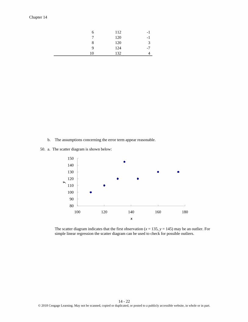
Chapter 14
14 - 22 © 2018 Cengage Learning. May not be scanned, copied or duplicated, or posted to a publicly accessible website, in whole or in part.
b. The assumptions concerning the error term appear reasonable. 50. a. The scatter diagram is shown below:
The scatter diagram indicates that the first observation (x = 135, y = 145) may be an outlier. For simple linear regression the scatter diagram can be used to check for possible outliers.
80
90
100
110
120
130
140
150
100 120 140 160 180
y
x
6 112 -1 7 120 -1 8 120 3 9 124 -7
10 132 4
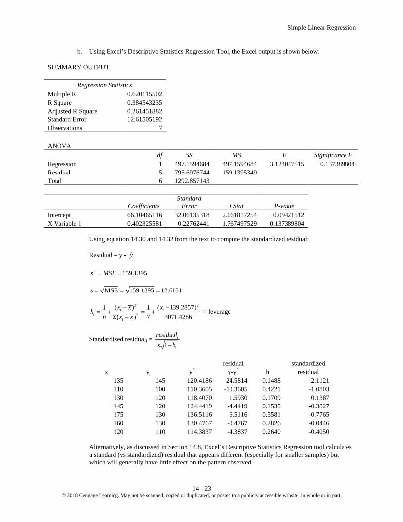
Simple Linear Regression
14 - 23 © 2018 Cengage Learning. May not be scanned, copied or duplicated, or posted to a publicly accessible website, in whole or in part.
b. Using Excel’s Descriptive Statistics Regression Tool, the Excel output is shown below:
SUMMARY OUTPUT
Regression Statistics Multiple R 0.620115502
R Square 0.384543235 Adjusted R Square 0.261451882 Standard Error 12.61505192 Observations 7
ANOVA df SS MS F Significance F
Regression 1 497.1594684 497.1594684 3.124047515 0.137389804 Residual 5 795.6976744 159.1395349
Total 6 1292.857143
Coefficients
Standard Error t Stat P-value
Intercept 66.10465116 32.06135318 2.061817254 0.09421512 X Variable 1 0.402325581 0.22762441 1.767497529 0.137389804
Using equation 14.30 and 14.32 from the text to compute the standardized residual: Residual = y - y 2 159.1395s MSE= = MSE 159.1395 12.6151s = = =
2 2
2
( ) ( 139.2857)1 17 3071.4286( )
i ii
i
x x xh
n x x− −
= + = +Σ −
= leverage
Standardized residuali = 1
i
i
residuals h−
residual
standardized
x y y^ y-y^ h residual 135 145 120.4186 24.5814 0.1488 2.1121 110 100 110.3605 -10.3605 0.4221 -1.0803 130 120 118.4070 1.5930 0.1709 0.1387 145 120 124.4419 -4.4419 0.1535 -0.3827 175 130 136.5116 -6.5116 0.5581 -0.7765 160 130 130.4767 -0.4767 0.2826 -0.0446 120 110 114.3837 -4.3837 0.2640 -0.4050
Alternatively, as discussed in Section 14.8, Excel’s Descriptive Statistics Regression tool calculates
a standard (vs standardized) residual that appears different (especially for smaller samples) but which will generally have little effect on the pattern observed.
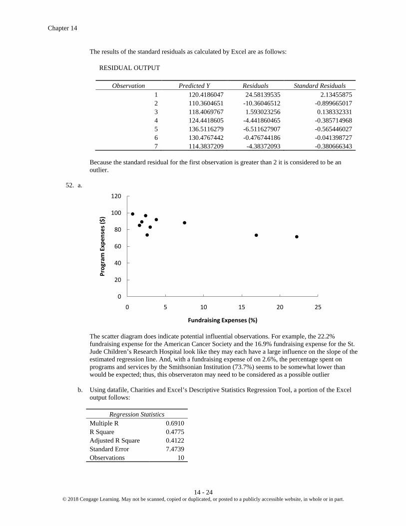
Chapter 14
14 - 24 © 2018 Cengage Learning. May not be scanned, copied or duplicated, or posted to a publicly accessible website, in whole or in part.
The results of the standard residuals as calculated by Excel are as follows:
RESIDUAL OUTPUT
Observation Predicted Y Residuals Standard Residuals 1 120.4186047 24.58139535 2.13455875 2 110.3604651 -10.36046512 -0.899665017 3 118.4069767 1.593023256 0.138332331 4 124.4418605 -4.441860465 -0.385714968 5 136.5116279 -6.511627907 -0.565446027 6 130.4767442 -0.476744186 -0.041398727 7 114.3837209 -4.38372093 -0.380666343
Because the standard residual for the first observation is greater than 2 it is considered to be an
outlier. 52. a.
The scatter diagram does indicate potential influential observations. For example, the 22.2%
fundraising expense for the American Cancer Society and the 16.9% fundraising expense for the St. Jude Children’s Research Hospital look like they may each have a large influence on the slope of the estimated regression line. And, with a fundraising expense of on 2.6%, the percentage spent on programs and services by the Smithsonian Institution (73.7%) seems to be somewhat lower than would be expected; thus, this observeraton may need to be considered as a possible outlier
b. Using datafile, Charities and Excel’s Descriptive Statistics Regression Tool, a portion of the Excel
output follows:
Regression Statistics Multiple R 0.6910
R Square 0.4775 Adjusted R Square 0.4122 Standard Error 7.4739 Observations 10
0
20
40
60
80
100
120
0 5 10 15 20 25
Prog
ram
Exp
ense
s ($)
Fundraising Expenses (%)
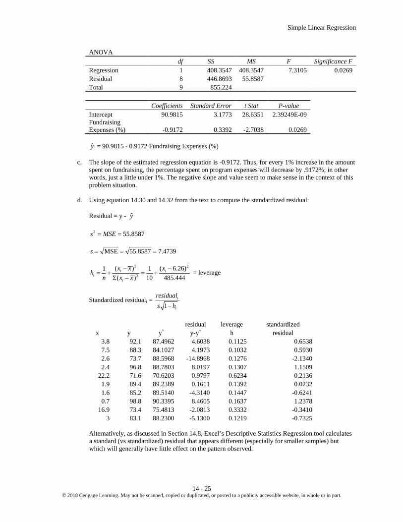
Simple Linear Regression
14 - 25 © 2018 Cengage Learning. May not be scanned, copied or duplicated, or posted to a publicly accessible website, in whole or in part.
ANOVA df SS MS F Significance F
Regression 1 408.3547 408.3547 7.3105 0.0269 Residual 8 446.8693 55.8587
Total 9 855.224
Coefficients Standard Error t Stat P-value Intercept 90.9815 3.1773 28.6351 2.39249E-09
Fundraising Expenses (%) -0.9172 0.3392 -2.7038 0.0269
y = 90.9815 - 0.9172 Fundraising Expenses (%) c. The slope of the estimated regression equation is -0.9172. Thus, for every 1% increase in the amount
spent on fundraising, the percentage spent on program expenses will decrease by .9172%; in other words, just a little under 1%. The negative slope and value seem to make sense in the context of this problem situation.
d. Using equation 14.30 and 14.32 from the text to compute the standardized residual: Residual = y - y 2 55.8587s MSE= = MSE 55.8587 7.4739s = = =
2 2
2
( ) ( 6.26)1 110 485.444( )
i ii
i
x x xh
n x x− −
= + = +Σ −
= leverage
Standardized residuali = 1
i
i
residuals h−
residual leverage standardized
x y y^ y-y^ h residual 3.8 92.1 87.4962 4.6038 0.1125 0.6538 7.5 88.3 84.1027 4.1973 0.1032 0.5930 2.6 73.7 88.5968 -14.8968 0.1276 -2.1340 2.4 96.8 88.7803 8.0197 0.1307 1.1509
22.2 71.6 70.6203 0.9797 0.6234 0.2136 1.9 89.4 89.2389 0.1611 0.1392 0.0232 1.6 85.2 89.5140 -4.3140 0.1447 -0.6241 0.7 98.8 90.3395 8.4605 0.1637 1.2378
16.9 73.4 75.4813 -2.0813 0.3332 -0.3410 3 83.1 88.2300 -5.1300 0.1219 -0.7325
Alternatively, as discussed in Section 14.8, Excel’s Descriptive Statistics Regression tool calculates
a standard (vs standardized) residual that appears different (especially for smaller samples) but which will generally have little effect on the pattern observed.

Chapter 14
14 - 26 © 2018 Cengage Learning. May not be scanned, copied or duplicated, or posted to a publicly accessible website, in whole or in part.
The results of the standard residuals as calculated by Excel are as follows:
RESIDUAL OUTPUT
Observation Predicted Y Residuals Standard Residuals 1 87.49623479 4.603765213 0.653347356 2 84.10271092 4.19728908 0.595661941 3 88.59683712 -14.89683712 -2.114097633 4 88.78027084 8.019729155 1.138126858 5 70.62033231 0.979667686 0.139030394 6 89.23885515 0.161144849 0.022869012 7 89.51400573 -4.314005735 -0.612225887 8 90.33945749 8.460542514 1.20068527 9 75.48132596 -2.081325961 -0.295373189
10 88.22996968 -5.129969677 -0.728024121 The standardized residuals from the Excel output and the calculated values for leverage are shown
below.
Charity Standard Residuals Leverage American Red Cross 0.6533 0.1125 World Vision 0.5957 0.1032 Smithsonian Institution -2.1141 0.1276 Food For The Poor 1.1381 0.1307 American Cancer Society 0.1390 0.6234 Volunteers of America 0.0229 0.1392 Dana-Farber Cancer Institute -0.6122 0.1447 AmeriCares 1.2007 0.1637 ALSAC - St. Jude Children's Research Hospital -0.2954 0.3332 City of Hope -0.7280 0.1219
• Observation 3 (Smithsonian Institution) is condiered to be an outlier because it has a large
standardized residual; standard residual = ˗2.1141 < ˗2.
• Observation 5 (American Cancer Society) is an influential observation because it has high leverage; leverage = .6234 > 6/10.
Although fundraising expenses for the Smithsonian Institution are on the low side as compared to
most of the other super-sized charities, the percentage spent on program expenses appears to be much lower than one would expect. It appears that the Smithsonian’s administrative expenses are too high. But, thinking about the expenses of running a large museum like the Smithsonian, the percentage spent on administrative expenses may not be unreasonable and is just due to the fact that operating costs for a museum are in general higher than for some other types of organizations. The very large value of fundraising expenses for the American Cancer Society suggests that this observation has a large influence on the estimated regression equation. The following Excel output shows the results if this observation is deleted from the original data.

Simple Linear Regression
14 - 27 © 2018 Cengage Learning. May not be scanned, copied or duplicated, or posted to a publicly accessible website, in whole or in part.
Regression Statistics Multiple R 0.5611
R Square 0.3149 Adjusted R Square 0.2170 Standard Error 7.9671 Observations 9
ANOVA df SS MS F Significance F
Regression 1 204.1814 204.1814 3.2168 0.1160 Residual 7 444.3209 63.4744
Total 8 648.5022
Coefficients Standard Error t Stat P-value Intercept 91.2561 3.6537 24.9766 4.207E-08
Fundraising Expenses (%) -1.0026 0.5590 -1.7935 0.1160
y = 91.2561 - 1.0026 Fundraising Expenses (%)
The y-intercept has changed slightly, but the slope has changed from -.917 to -1.0026.
54. a.
The scatter diagram does indicate potential outliers and/or influential observations. For example, the
New York Yankees have both the hightest revenue and value, and appears to be an influential observation. The Los Angeles Dodgers have the second highest value and appears to be an outlier.
0
500
1,000
1,500
2,000
2,500
0 100 200 300 400 500
Val
ue ($
mill
ions
)
Revenue ($ millions)

Chapter 14
14 - 28 © 2018 Cengage Learning. May not be scanned, copied or duplicated, or posted to a publicly accessible website, in whole or in part.
b. Using datafile, MLBValues and Excel’s Descriptive Statistics Regression Tool, a portion of the Excel output follows:
Regression Statistics Multiple R 0.9062
R Square 0.8211 Adjusted R Square 0.8148 Standard Error 165.6581 Observations 30
ANOVA df SS MS F Significance F
Regression 1 3527616.598 3527616.6 128.5453 5.616E-12 Residual 28 768392.7687 27442.599
Total 29 4296009.367
Coefficients Standard Error t Stat P-value Lower 95% Upper 95% Intercept -601.4814 122.4288 -4.9129 3.519E-05 -852.2655 -350.6973 Revenue ($ millions) 5.9271 0.5228 11.3378 5.616E-12 4.8562 6.9979
Thus, the estimated regression equation that can be used to predict the team’s value given the value
of annual revenue is y = -601.4814 + 5.9271 Revenue. c. Using Excel’s Data Analysis Regression Tool with standardized residuals out put, you find that the
Standard Residual value for the Los Angeles Dodgers is 4.7 and should be treated as an outlier. To determine if the New York Yankees point is an influential observation we can remove the observation and compute a new estimated regression equation. The results show that the estimated regresssion equation is y = -449.061 + 5.2122 Revenue. The following two scatter diagrams illustrate the small change in the estimated regression equation after removing the observation for the New York Yankees. These scatter diagrams show that the effect of the New York Yankees observation on the regression results is not that dramatic. (Note that leverage analysis will show that the leverage for the New York Yankees is h=.63 which does exceed 6/n = 6/30 = .2 and indicate the possibility of it as an influential observation.
Scatter Diagram Including the New York Yankees Observation

Simple Linear Regression
14 - 29 © 2018 Cengage Learning. May not be scanned, copied or duplicated, or posted to a publicly accessible website, in whole or in part.
Scatter Diagram Excluding the New York Yankees Observation
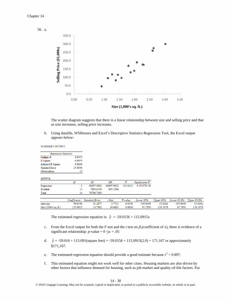
Chapter 14
14 - 30 © 2018 Cengage Learning. May not be scanned, copied or duplicated, or posted to a publicly accessible website, in whole or in part.
56. a.
The scatter diagram suggests that there is a linear relationship between size and selling price and that as size increases, selling price increases.
b. Using datafile, WSHouses and Excel’s Descriptive Statistics Regression Tool, the Excel output
appears below:
The estimated regression equation is: y = -59.0156 + 115.0915x c. From the Excel output for both the F test and the t test on β1(coefficient of x), there is evidence of a
significant relationship: p-value = 0 <α = .05
d. y = -59.016 + 115.091(square feet) = -59.0156 + 115.0915(2.0) = 171.167 or approximately $171,167. e. The estimated regression equation should provide a good estimate because r2 = 0.897. f. This estimated equation might not work well for other cities. Housing markets are also driven by
other factors that influence demand for housing, such as job market and quality-of-life factors. For
0.0
50.0
100.0
150.0
200.0
250.0
300.0
350.0
0.00 0.50 1.00 1.50 2.00 2.50 3.00 3.50
Selli
ng P
rice
($1,
000s
)
Size (1,000's sq. ft.)
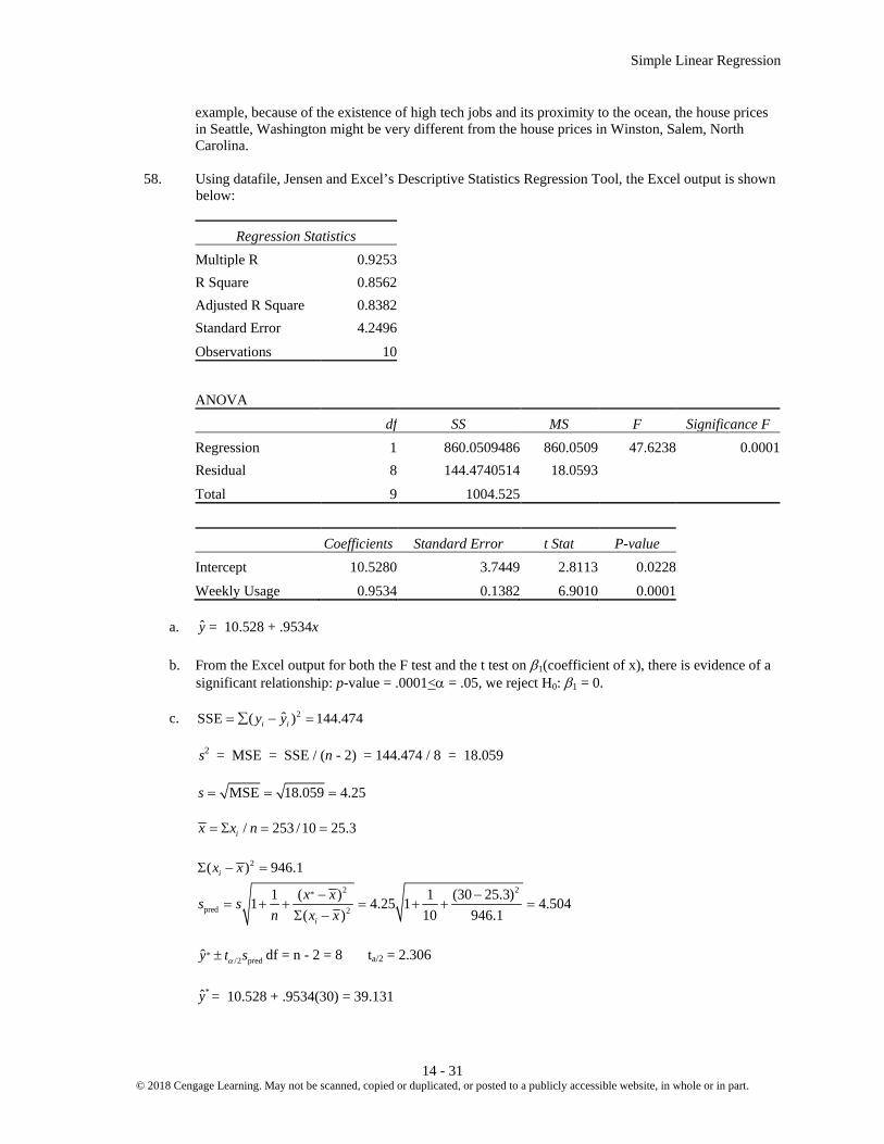
Simple Linear Regression
14 - 31 © 2018 Cengage Learning. May not be scanned, copied or duplicated, or posted to a publicly accessible website, in whole or in part.
example, because of the existence of high tech jobs and its proximity to the ocean, the house prices in Seattle, Washington might be very different from the house prices in Winston, Salem, North Carolina.
58. Using datafile, Jensen and Excel’s Descriptive Statistics Regression Tool, the Excel output is shown
below:
Regression Statistics Multiple R 0.9253 R Square 0.8562 Adjusted R Square 0.8382 Standard Error 4.2496
Observations 10
ANOVA
df SS MS F Significance F Regression 1 860.0509486 860.0509 47.6238 0.0001 Residual 8 144.4740514 18.0593
Total 9 1004.525
Coefficients Standard Error t Stat P-value Intercept 10.5280 3.7449 2.8113 0.0228
Weekly Usage 0.9534 0.1382 6.9010 0.0001 a. y = 10.528 + .9534x
b. From the Excel output for both the F test and the t test on β1(coefficient of x), there is evidence of a
significant relationship: p-value = .0001<α = .05, we reject H0: β1 = 0. c. 2ˆSSE ( ) 144.474i iy y= ∑ − =
s2 = MSE = SSE / (n - 2) = 144.474 / 8 = 18.059
MSE 18.059 4.25s = = = / 253 /10 25.3ix x n= Σ = =
2( ) 946.1ix xΣ − =
2 2*
pred 2
1 ( ) 1 (30 25.3)1 4.25 1 4.50410 946.1( )i
x xs sn x x
− −= + + = + + =
Σ −
*
/2 predy t sα± df = n - 2 = 8 ta/2 = 2.306 *y = 10.528 + .9534(30) = 39.131

Chapter 14
14 - 32 © 2018 Cengage Learning. May not be scanned, copied or duplicated, or posted to a publicly accessible website, in whole or in part.
39.131± 2.306(4.504) = 39.131± 10.386 The 95% prediction interval is 28.74 to 49.52 or $2874 to $4952 d. Yes, since the predicted expense fr 30 hours is $3913. Therefore, a $3000 contract should save money. 60. a. Using datafile, HoursPts and Excel’s Descriptive Statistics Regression Tool, the Excel output follows:
y = 5.847 + .8295(Hours) = 5.847 + .8295x
b. From the Excel output for both the F test and the t test on β1(coefficient of x), there is evidence of a
significant relationship: p-value = .0001<α =.05, we reject H0: β1 = 0. Total points earned is related to the hours spent studying. c. Points = 5.8470 + .8295 Hours = 5.8470 + .8295 (95) = 84.65 points d. 2ˆSSE ( ) 452.779i iy y= ∑ − =
s2 = MSE = SSE / (n - 2) = 452.779 / 8 = 56.597
MSE 56.597 7.523s = = = / 695 /10 69.5ix x n= Σ = =
2( ) 4722.5ix xΣ − =
2 2*
pred 2
1 ( ) 1 (95 69.5)1 7.523 1 8.37010 4722.5( )i
x xs sn x x
− −= + + = + + =
Σ −
*/2 predy t sα± df = n - 2 = 8 ta/2 = 2.306
*y = 5.847 + .8295(95) = 84.653 84.653± 2.306(8.37) = 84.653±19.3

Simple Linear Regression
14 - 33 © 2018 Cengage Learning. May not be scanned, copied or duplicated, or posted to a publicly accessible website, in whole or in part.
The 95% prediction interval is 65.353 to 103.954 62 a.
b. There appears to be a positive linear relationship between the two variables. c. Using datafile, AirlineSeats and Excel’s Descriptive Statistics Regression Tool, the Excel output is
shown below.
Regression Statistics Multiple R 0.8702
R Square 0.7572 Adjusted R Square 0.7456 Standard Error 11.5916 Observations 23
ANOVA df SS MS F Significance F
Regression 1 8798.2391 8798.2391 65.4802 6.85277E-08 Residual 21 2821.6609 134.3648
Total 22 11619.9 Coefficients Standard Error t Stat P-value
Intercept 7.3880 8.2125 0.8996 0.3785 2011 Percentage 0.9276 0.1146 8.0920 6.85277E-08
y = 7.3880 + 0.9276(2011 Percentage) d. From the Excel output for both the F test and the t test on β1(coefficient of x), there is evidence of a
significant relationship: p-value = 0.000 <α = .05. e. 2r = .7572; a good fit.
0.0
20.0
40.0
60.0
80.0
100.0
120.0
0.0 20.0 40.0 60.0 80.0 100.0 120.0
2012
Per
cent
age
2011 Percentage

Chapter 14
14 - 34 © 2018 Cengage Learning. May not be scanned, copied or duplicated, or posted to a publicly accessible website, in whole or in part.
f.
The point with a residual value of approximately 36 clearly stands out as compared to the other
points. This point corresponds to the observation for Air Tran Airways. Other than this point, the residual plot does not exhibit a pattern that would suggest a linear model is not appropriate.
-30
-20
-10
0
10
20
30
40
0.0 20.0 40.0 60.0 80.0 100.0 120.0
Resi
dual
s
2011 Percentage

15 - 1 © 2018 Cengage Learning. May not be scanned, copied or duplicated, or posted to a publicly accessible website, in whole or in part.
Chapter 15 Multiple Regression Solutions: 2. a. Using datafile Exer2 and Excel’s Descriptive Statistics Regression Tool, the Excel output is shown
below:
Regression Statistics Multiple R 0.8124 R Square 0.6600 Adjusted R Square 0.6175 Standard Error 25.4009
Observations 10
ANOVA
df SS MS F Significance F Regression 1 10021.24739 10021.25 15.5318 0.0043 Residual 8 5161.652607 645.2066
Total 9 15182.9
Coefficients Standard Error t Stat P-value Intercept 45.0594 25.4181 1.7727 0.1142
X1 1.9436 0.4932 3.9410 0.0043 An estimate of y when x1 = 45 is y = 45.0594 + 1.9436(45) = 132.52 b. Using datafile Exer2 and Excel’s Descriptive Statistics Regression Tool, the Excel output is shown
below:
Regression Statistics Multiple R 0.4707 R Square 0.2215 Adjusted R Square 0.1242 Standard Error 38.4374
Observations 10
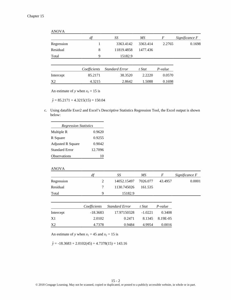
Chapter 15
15 - 2 © 2018 Cengage Learning. May not be scanned, copied or duplicated, or posted to a publicly accessible website, in whole or in part.
ANOVA
df SS MS F Significance F Regression 1 3363.4142 3363.414 2.2765 0.1698 Residual 8 11819.4858 1477.436
Total 9 15182.9
Coefficients Standard Error t Stat P-value Intercept 85.2171 38.3520 2.2220 0.0570
X2 4.3215 2.8642 1.5088 0.1698 An estimate of y when x2 = 15 is y = 85.2171 + 4.3215(15) = 150.04 c. Using datafile Exer2 and Excel’s Descriptive Statistics Regression Tool, the Excel output is shown
below:
Regression Statistics Multiple R 0.9620 R Square 0.9255 Adjusted R Square 0.9042 Standard Error 12.7096
Observations 10
ANOVA
df SS MS F Significance F Regression 2 14052.15497 7026.077 43.4957 0.0001 Residual 7 1130.745026 161.535
Total 9 15182.9
Coefficients Standard Error t Stat P-value Intercept -18.3683 17.97150328 -1.0221 0.3408 X1 2.0102 0.2471 8.1345 8.19E-05
X2 4.7378 0.9484 4.9954 0.0016 An estimate of y when x1 = 45 and x2 = 15 is y = -18.3683 + 2.0102(45) + 4.7378(15) = 143.16

Multiple Regression
15 - 3 © 2018 Cengage Learning. May not be scanned, copied or duplicated, or posted to a publicly accessible website, in whole or in part.
4. a. y = 25 + 10(15) + 8(10) = 255; sales estimate: $255,000 b. Sales can be expected to increase by $10 for every dollar increase in inventory investment when
advertising expenditure is held constant. Sales can be expected to increase by $8 for every dollar increase in advertising expenditure when inventory investment is held constant.
5. a. Using datafile Showtime and Excel’s Descriptive Statistics Regression Tool, the Excel output is
shown below:
Regression Statistics Multiple R 0.8078 R Square 0.6526 Adjusted R Square 0.5946 Standard Error 1.2152 Observations 8 ANOVA
df SS MS F Significance F Regression 1 16.6401 16.6401 11.2688 0.0153 Residual 6 8.8599 1.4767 Total 7 25.5
Coefficients Standard Error t Stat P-value Intercept 88.6377 1.5824 56.0159 2.174E-09 Television Advertising ($1000s) 1.6039 0.4778 3.3569 0.0153
y = 88.6377 + 1.6039x1 wherex1 = television advertising ($1000s) b. Using datafile Showtime and Excel’s Descriptive Statistics Regression Tool, the Excel output is
shown below:
Regression Statistics Multiple R 0.9587 R Square 0.9190 Adjusted R Square 0.8866 Standard Error 0.6426 Observations 8 ANOVA
df SS MS F Significance F Regression 2 23.4354 11.7177 28.3778 0.0019 Residual 5 2.0646 0.4129 Total 7 25.5
Coefficients Standard Error t Stat P-value Intercept 83.2301 1.5739 52.8825 4.57E-08
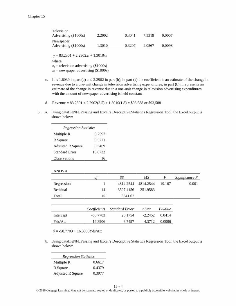
Chapter 15
15 - 4 © 2018 Cengage Learning. May not be scanned, copied or duplicated, or posted to a publicly accessible website, in whole or in part.
Television Advertising ($1000s) 2.2902 0.3041 7.5319 0.0007 Newspaper Advertising ($1000s) 1.3010 0.3207 4.0567 0.0098
y = 83.2301 + 2.2902x1 + 1.3010x2 where x1 = television advertising ($1000s) x2 = newspaper advertising ($1000s) c. It is 1.6039 in part (a) and 2.2902 in part (b); in part (a) the coefficient is an estimate of the change in
revenue due to a one-unit change in television advertising expenditures; in part (b) it represents an estimate of the change in revenue due to a one-unit change in television advertising expenditures with the amount of newspaper advertising is held constant
d. Revenue = 83.2301 + 2.2902(3.5) + 1.3010(1.8) = $93.588 or $93,588 6. a. Using datafileNFLPassing and Excel’s Descriptive Statistics Regression Tool, the Excel output is
shown below:
Regression Statistics Multiple R 0.7597
R Square 0.5771 Adjusted R Square 0.5469 Standard Error 15.8732 Observations 16
ANOVA df SS MS F Significance F
Regression 1 4814.2544 4814.2544 19.107 0.001 Residual 14 3527.4156 251.9583
Total 15 8341.67
Coefficients Standard Error t Stat P-value Intercept -58.7703 26.1754 -2.2452 0.0414
Yds/Att 16.3906 3.7497 4.3712 0.0006
y = -58.7703 + 16.3906Yds/Att b. Using datafileNFLPassing and Excel’s Descriptive Statistics Regression Tool, the Excel output is
shown below:
Regression Statistics Multiple R 0.6617
R Square 0.4379 Adjusted R Square 0.3977

Multiple Regression
15 - 5 © 2018 Cengage Learning. May not be scanned, copied or duplicated, or posted to a publicly accessible website, in whole or in part.
Standard Error 18.3008 Observations 16
ANOVA df SS MS F Significance F
Regression 1 3652.8003 3652.8003 10.9065 0.0052 Residual 14 4688.8697 334.9193
Total 15 8341.67
Coefficients Standard Error t Stat P-value Intercept 97.5383 13.8618 7.0365 5.898E-06
Int/Att -1600.491 484.6300 -3.3025 0.0052
y = 97.5383 – 1600.491Int/Att c. Using datafileNFLPassing and Excel’s Descriptive Statistics Regression Tool, the Excel output is
shown below:
Regression Statistics Multiple R 0.8675
R Square 0.7525 Adjusted R Square 0.7144 Standard Error 12.6024 Observations 16
ANOVA df SS MS F Significance F
Regression 2 6277.0142 3138.5071 19.7614 0.0001 Residual 13 2064.6558 158.8197
Total 15 8341.67
Coefficients Standard Error t Stat P-value Intercept -5.7633 27.1468 -0.2123 0.8352
Yds/Att 12.9494 3.1857 4.0649 0.0013 Int/Att -1083.7880 357.1165 -3.0348 0.0096
y = -5.7633 + 12.9494Yds/Att - 1083.7880 Int/Att d. The predicted value of Win% for the Kansas City Chiefs is Win% = -5.7633 + 12.9494(6.2) - 1083.7880(.036) = 35.5% With 7 wins and 9 loses, the Kansas City Chiefs won 43.75% of the games they played. The
predicted value is somewhat lower than the actual value.
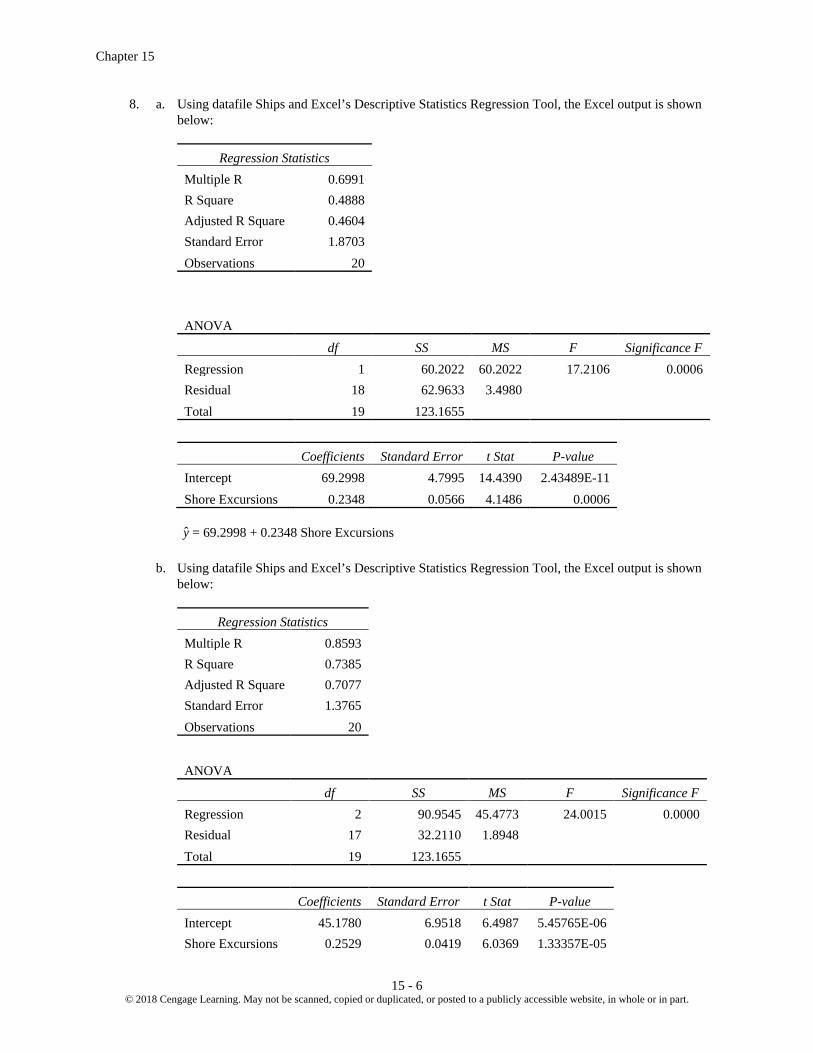
Chapter 15
15 - 6 © 2018 Cengage Learning. May not be scanned, copied or duplicated, or posted to a publicly accessible website, in whole or in part.
8. a. Using datafile Ships and Excel’s Descriptive Statistics Regression Tool, the Excel output is shown below:
Regression Statistics Multiple R 0.6991
R Square 0.4888 Adjusted R Square 0.4604 Standard Error 1.8703 Observations 20
ANOVA
df SS MS F Significance F Regression 1 60.2022 60.2022 17.2106 0.0006 Residual 18 62.9633 3.4980
Total 19 123.1655
Coefficients Standard Error t Stat P-value Intercept 69.2998 4.7995 14.4390 2.43489E-11
Shore Excursions 0.2348 0.0566 4.1486 0.0006
y = 69.2998 + 0.2348 Shore Excursions b. Using datafile Ships and Excel’s Descriptive Statistics Regression Tool, the Excel output is shown
below:
Regression Statistics Multiple R 0.8593
R Square 0.7385 Adjusted R Square 0.7077 Standard Error 1.3765 Observations 20
ANOVA df SS MS F Significance F
Regression 2 90.9545 45.4773 24.0015 0.0000 Residual 17 32.2110 1.8948
Total 19 123.1655
Coefficients Standard Error t Stat P-value Intercept 45.1780 6.9518 6.4987 5.45765E-06
Shore Excursions 0.2529 0.0419 6.0369 1.33357E-05

Multiple Regression
15 - 7 © 2018 Cengage Learning. May not be scanned, copied or duplicated, or posted to a publicly accessible website, in whole or in part.
Food/Dining 0.2482 0.0616 4.0287 0.0009
y = 45.1780 + 0.2529 Shore Excursions + 0.2482 Food/Dining c. The predicted score is y = 45.1780 + 0.2529(80) + 0.2482(90) = 87.75 or approximately 88 10. a. Using datafileMLBPitching and Excel’s Descriptive Statistics Regression Tool, the Excel output
follows.
Regression Statistics Multiple R 0.6477
R Square 0.4195 Adjusted R Square 0.3873 Standard Error 0.0603 Observations 20
ANOVA df SS MS F Significance F
Regression 1 0.0473 0.0473 13.0099 0.0020 Residual 18 0.0654 0.0036
Total 19 0.1127
Coefficients Standard Error t Stat P-value Intercept 0.6758 0.0631 10.7135 3.06093E-09
SO/IP -0.2838 0.0787 -3.6069 0.0020
y = 0.6758 ˗ 0.2838 SO/IP
b. Using datafileMLBPitching and Excel’s Descriptive Statistics Regression Tool, the Excel output follows.
Regression Statistics Multiple R 0.5063
R Square 0.2563 Adjusted R Square 0.2150 Standard Error 0.0682 Observations 20
ANOVA df SS MS F Significance F
Regression 1 0.0289 0.0289 6.2035 0.0227
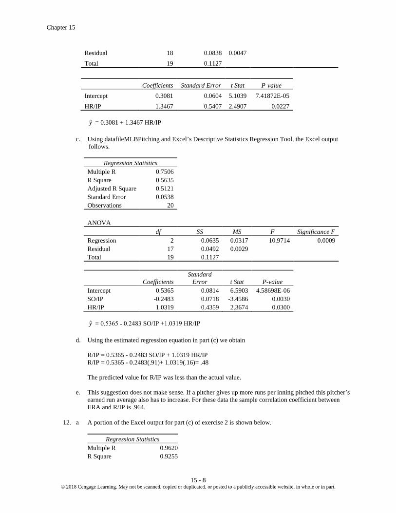
Chapter 15
15 - 8 © 2018 Cengage Learning. May not be scanned, copied or duplicated, or posted to a publicly accessible website, in whole or in part.
Residual 18 0.0838 0.0047 Total 19 0.1127
Coefficients Standard Error t Stat P-value Intercept 0.3081 0.0604 5.1039 7.41872E-05
HR/IP 1.3467 0.5407 2.4907 0.0227
y = 0.3081 + 1.3467 HR/IP
c. Using datafileMLBPitching and Excel’s Descriptive Statistics Regression Tool, the Excel output follows.
Regression Statistics
Multiple R 0.7506 R Square 0.5635 Adjusted R Square 0.5121 Standard Error 0.0538 Observations 20
ANOVA df SS MS F Significance F
Regression 2 0.0635 0.0317 10.9714 0.0009 Residual 17 0.0492 0.0029
Total 19 0.1127
Coefficients
Standard Error t Stat P-value
Intercept 0.5365 0.0814 6.5903 4.58698E-06 SO/IP -0.2483 0.0718 -3.4586 0.0030 HR/IP 1.0319 0.4359 2.3674 0.0300
y = 0.5365 ˗ 0.2483 SO/IP +1.0319 HR/IP d. Using the estimated regression equation in part (c) we obtain R/IP = 0.5365 - 0.2483 SO/IP + 1.0319 HR/IP R/IP = 0.5365 - 0.2483(.91)+ 1.0319(.16)= .48 The predicted value for R/IP was less than the actual value. e. This suggestion does not make sense. If a pitcher gives up more runs per inning pitched this pitcher’s
earned run average also has to increase. For these data the sample correlation coefficient between ERA and R/IP is .964.
12. a A portion of the Excel output for part (c) of exercise 2 is shown below.
Regression Statistics Multiple R 0.9620 R Square 0.9255

Multiple Regression
15 - 9 © 2018 Cengage Learning. May not be scanned, copied or duplicated, or posted to a publicly accessible website, in whole or in part.
Adjusted R Square 0.9042 Standard Error 12.7096 Observations 10
. 2 SSR 14,052.2 .9255SST 15,182.9
R = = =
b. 2 2 1 10 11 (1 ) 1 (1 .9255) .90421 10 2 1a
nR Rn p
− −= − − = − − =
− − − −
c. Yes; after adjusting for the number of independent variables in the model, we see that 90.42% of the
variability in y has been accounted for.
14. a. 2 SSR 12,000 .75SST 16,000
R = = =
b. 2 2 1 10 11 (1 ) 1 (1 .75) .67861 10 2 1a
nR Rn p
− −= − − = − − =
− − − −
c. The adjusted coefficient of determination shows that 67.86% of the variability has been explained by
the two independent variables; thus, we conclude that the model does not explain a large amount of variability.
15. a. A portion of the Excel output for part (b) of exercise 5 is shown below.
Regression Statistics Multiple R 0.9587 R Square 0.9190 Adjusted R Square 0.8866 Standard Error 0.6426 Observations 8
2 SSR 23.435 .9190SST 25.5
R = = =
2 2 1 8 11 (1 ) 1 (1 .9190) .88661 8 2 1a
nR Rn p
− −= − − = − − =
− − − −
b. Multiple regression analysis is preferred since both R2 and 2aR show an increased percentage of the
variability of y explained when both independent variables are used. 16. a. A portion of the Excel output for part (a) of exercise 6 is shown below.
Regression Statistics Multiple R 0.7597
R Square 0.5771 Adjusted R Square 0.5469 Standard Error 15.8732 Observations 16
R2 = .5771. Thus, the averages number of passing yards per attempt is able to explain 57.71% of the

Chapter 15
15 - 10 © 2018 Cengage Learning. May not be scanned, copied or duplicated, or posted to a publicly accessible website, in whole or in part.
variability in the percentage of games won. Considering the nature of the data and all the other factors that might be related to the number of games won, this is not too bad a fit.
b. A portion of the Excel output for part (c) of exercise 6 is shown below.
Regression Statistics Multiple R 0.8675
R Square 0.7525 Adjusted R Square 0.7144 Standard Error 12.6024 Observations 16
The value of the coefficient of determination increased to R2 = .7525, and the adjusted coefficient of determination is 2
aR = .7144. Thus, using both independent variables provides a much better fit. 18. a. A portion of the Excel output for part (c) of exercise 10 is shown below.
Regression Statistics Multiple R 0.7506
R Square 0.5635 Adjusted R Square 0.5121 Standard Error 0.0538 Observations 20
The value of R2= .5635 and the value of 2aR = .5121.
b. The fit is not great, but considering the nature of the data being able to explain slightly more than
50% of the variability in the number of runs given up per inning pitched using just two independent variables is not too bad.
c. Using datafileMLBPitching and Excel’s Descriptive Statistics Regression Tool, the Excel output is
shown below.
Regression Statistics Multiple R 0.7907
R Square 0.6251 Adjusted R Square 0.5810 Standard Error 0.4272 Observations 20
ANOVA df SS MS F Significance F
Regression 2 5.1739 2.5870 14.1750 0.0002 Residual 17 3.1025 0.1825
Total 19 8.2765
Coefficients
Standard Error t Stat P-value
Intercept 3.8781 0.6466 5.9976 1.44078E-05 SO/IP -1.8428 0.5703 -3.2310 0.0049 HR/IP 11.9933 3.4621 3.4641 0.0030

Multiple Regression
15 - 11 © 2018 Cengage Learning. May not be scanned, copied or duplicated, or posted to a publicly accessible website, in whole or in part.
The Excel output shows that 2R = .6251 and 2
aR = .5810 Approximately 60% of the variability in the ERA can be explained by the linear effect of HR/IP and
SO/IP. This is not too bad considering the complexity of predicting pitching performance. 19. a. SSE = SST - SSR = 6724.125 – 6216.375 = 507.75 MSR = SSR/p = 6,216.375/2 = 3,108.1875
SSE 507.75MSE 72.53571 10 2 1n p
= = =− − − −
b. F = MSR/MSE = 3,108.1875/72.5357 = 42.85 Using F Table(2 degrees of freedom numerator and 7 denominator), p-value is less than .01. Using Excel, the p-value = F.DIST.RT(42.85,2,7) = .0001 Because the p-value ≤ α = .05, the overall model is significant.
c. .5906 7.26.0813
i
i
b
bt
s= = =
Degrees of freedom = n – p - 1 = 7
Because t> 0, p-value is two times the upper tail area Using t table; area in upper tail is less than .005; therefore, p-value is less than .01. Using Excel: p-value = 2*(1-T.DIST(7.26,7,TRUE)) = .0002 Because the p-value ≤ α = .05, β1 is significant.
d. .4980 8.78.0567
i
i
b
bt
s= = =
Degrees of freedom = n – p - 1 = 7
Because t> 0, p-value is two times the upper tail area Using t table; area in upper tail is less than .005; therefore, p-value is less than .01. Using Excel: p-value = 2*(1-T.DIST(8.78,7,TRUE)) = .0001 Because the p-value ≤ α = .05, β2 is significant. 20. A portion of the Excel output for part (c) of exercise 2 is shown below.
Regression Statistics Multiple R 0.9620 R Square 0.9255 Adjusted R Square 0.9042 Standard Error 12.7096 Observations 10
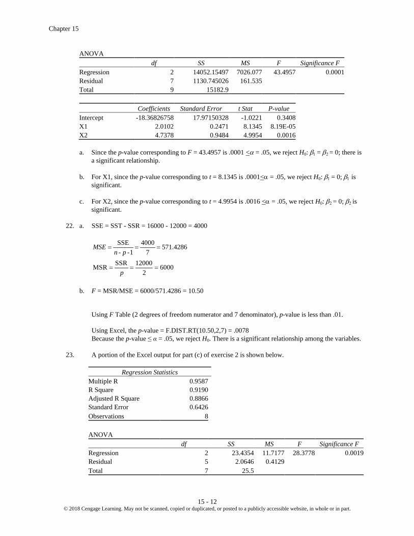
Chapter 15
15 - 12 © 2018 Cengage Learning. May not be scanned, copied or duplicated, or posted to a publicly accessible website, in whole or in part.
ANOVA df SS MS F Significance F
Regression 2 14052.15497 7026.077 43.4957 0.0001 Residual 7 1130.745026 161.535 Total 9 15182.9
Coefficients Standard Error t Stat P-value Intercept -18.36826758 17.97150328 -1.0221 0.3408 X1 2.0102 0.2471 8.1345 8.19E-05 X2 4.7378 0.9484 4.9954 0.0016
a. Since the p-value corresponding to F = 43.4957 is .0001 <α = .05, we reject H0: β1 = β2 = 0; there is
a significant relationship. b. For X1, since the p-value corresponding to t = 8.1345 is .0001<α = .05, we reject H0: β1 = 0; β1 is
significant. c. For X2, since the p-value corresponding to t = 4.9954 is .0016 <α = .05, we reject H0: β2 = 0; β2 is
significant. 22. a. SSE = SST - SSR = 16000 - 12000 = 4000
SSE 4000 571.4286- -1 7
MSEn p
= = =
SSR 12000MSR 60002p
= = =
b. F = MSR/MSE = 6000/571.4286 = 10.50 Using F Table (2 degrees of freedom numerator and 7 denominator), p-value is less than .01. Using Excel, the p-value = F.DIST.RT(10.50,2,7) = .0078 Because the p-value ≤ α = .05, we reject H0. There is a significant relationship among the variables. 23. A portion of the Excel output for part (c) of exercise 2 is shown below.
Regression Statistics Multiple R 0.9587 R Square 0.9190 Adjusted R Square 0.8866 Standard Error 0.6426 Observations 8 ANOVA
df SS MS F Significance F Regression 2 23.4354 11.7177 28.3778 0.0019 Residual 5 2.0646 0.4129 Total 7 25.5

Multiple Regression
15 - 13 © 2018 Cengage Learning. May not be scanned, copied or duplicated, or posted to a publicly accessible website, in whole or in part.
Coefficients Standard Error t Stat P-value Intercept 83.2301 1.5739 52.8825 4.57E-08 Television Advertising ($1000s) 2.2902 0.3041 7.5319 0.0007 Newspaper Advertising ($1000s) 1.3010 0.3207 4.0567 0.0098
a. Since the p-value corresponding to F = 28.3778 is .0019≤ α = .01, we reject H0. : β1 = β2 = 0; there is a significant relationship.
b. For Television Advertising, since the p-value corresponding to t = 7.5319 is .0007 <α = .05, we
reject H0: β1 = 0; β1 is significantand x1 should not be dropped from the model. c. For Newspaper Advertising, since the p-value corresponding to t = 4.0567 is .0098 <α = .05, we reject H0: β2 = 0; β2 is significant and x2 should not be dropped from the model. 24. a. Using datafile NFL2011 and Excel’s Descriptive Statistics Regression Tool, the Excel output is
shown below:
Regression Statistics Multiple R 0.6901
R Square 0.4762 Adjusted R Square 0.4401 Standard Error 15.3096 Observations 32
ANOVA df SS MS F Significance F
Regression 2 6179.1015 3089.5507 13.1815 8.47389E-05 Residual 29 6797.1673 234.3851
Total 31 12976.2688
Coefficients Standard Error t Stat P-value Intercept 60.5405 28.3562 2.1350 0.0413
OffPassYds/G 0.3186 0.0626 5.0929 1.95917E-05 DefYds/G -0.2413 0.0893 -2.7031 0.0114
y = 60.5405 + 0.3186 OffPassYds/G ˗0.2413 DefYds/G b. With F=13.1815, the p-value for the F test = .0001<α = .05, there is a significant relationship. c. For OffPassYds/G, t=5.0929: Because the p-value = .0000<α = .05, OffPassYds/G is significant. For DefYds/G, t=-2.7031: Because the p-value = .0114<α = .05, DefYds/G is significant. 26. The Excel output from part (c) of exercise 10 follows.
Regression Statistics Multiple R 0.7506
R Square 0.5635

Chapter 15
15 - 14 © 2018 Cengage Learning. May not be scanned, copied or duplicated, or posted to a publicly accessible website, in whole or in part.
Adjusted R Square 0.5121 Standard Error 0.0538 Observations 20
ANOVA df SS MS F Significance F
Regression 2 0.0635 0.0317 10.9714 0.0009 Residual 17 0.0492 0.0029
Total 19 0.1127
Coefficients
Standard Error t Stat P-value
Intercept 0.5365 0.0814 6.5903 4.58698E-06 SO/IP -0.2483 0.0718 -3.4586 0.0030 HR/IP 1.0319 0.4359 2.3674 0.0300
a. The p-value associated with F = 10.9714 is .0009. Because the p-value < .05, there is a significant overall relationship.
b. For SO/IP, the p-value associated with t = -3.4586 is .0030. Because the p-value <.05, SO/IP is
significant. For HR/IP, thep-value associated with t = 2.3674 is .0300. Because the p-value < .05, HR/IP is also significant.
28. a. y = -18.4 + 2.01(45) + 4.74(15) = 143.15 or 143.16 from unrounded equation values and StatTools
output. b. Using StatTools with Exer2 datafile, the 95% prediction interval is 111.16 to 175.16. 29. a. y = 83.2 + 2.29(3.5) + 1.30(1.8) = 93.555 or $93,555 or 93.588 or $93,588 from unrounded
equation values and StatTools output (also ties to exercise 5d) b. Using StatTools with Showtime datafile, the prediction interval estimate: 91.774 to 95.401 or $91,774 to $95,401 30. a. A portion of the Excel output form Exercise 24 is shown below:
Coefficients Standard Error t Stat P-value Intercept 60.5405 28.3562 2.1350 0.0413
OffPassYds/G 0.3186 0.0626 5.0929 1.95917E-05 DefYds/G -0.2413 0.0893 -2.7031 0.0114
The estimated regression equation is y = 60.5405 + 0.3186 OffPassYds/G ˗ 0.2413 DefYds/G
For OffPassYds/G = 225 and DefYds/G = 300, the predicted value of the percentage of games won is y = 60.5405 + 0.3186(225) ˗ 0.2413(300) = 59.827

Multiple Regression
15 - 15 © 2018 Cengage Learning. May not be scanned, copied or duplicated, or posted to a publicly accessible website, in whole or in part.
b. Using StatTools with NFL2011 datafile, the 95% prediction interval is 26.959 to 92.695 or 27.0 to 92.7
32. a. E(y) = β0 + β1 x1 + β2 x2wherex2= 0 if level 1 and 1 if level 2 b. E(y) = β0 + β1 x1 + β2(0) = β0 + β1 x1 c. E(y) = β0 + β1 x1 + β2(1) = β0 + β1 x1 + β2 d. β1 is the change in E(y) for a 1 unit change in x1holding x2 constant. β2 = E(y | level 2) - E(y | level 1) 34. a. $15,300 which equals the coefficient of variable 3 b. Estimate of sales = 10.1 - 4.2(2) + 6.8(8) + 15.3(0) = 56.1 or $56,100 c. Estimate of sales = 10.1 - 4.2(1) + 6.8(3) + 15.3(1) = 41.6 or $41,600 36. a. Using datafile Repair and Excel’s Descriptive Statistics Regression Tool, the Excel output is shown
below:
Regression Statistics Multiple R 0.9488 R Square 0.900199692 Adjusted R Square 0.850299539 Standard Error 0.4174 Observations 10 ANOVA
df SS MS F Significance F Regression 3 9.4305 3.1435 18.0400 0.0021 Residual 6 1.0455 0.1743 Total 9 10.476
Coefficients Standard Error t Stat P-value Intercept 1.8602 0.7286 2.5529 0.0433 Months Since Last Service 0.2914 0.0836 3.4862 0.0130 Type 1.1024 0.3033 3.6342 0.0109 Person -0.6091 0.3879 -1.5701 0.1674
y = 1.8602 + .2914 Months + 1.1024 Type - .6091 Person b. Since the p-value corresponding to F = 18.04 is .0021 <α = .05, the overall model is statistically
significant. c. The p-value corresponding to t = -1.5701 is .1674 >α = .05; thus, the addition of Person is not
statistically significant. Person is highly correlated with Months (the sample correlation coefficient is -.691); thus, once the effect of Months has been accounted for, Person will not add much to the model.

Chapter 15
15 - 16 © 2018 Cengage Learning. May not be scanned, copied or duplicated, or posted to a publicly accessible website, in whole or in part.
38. a. Using datafile Stroke and Excel’s Descriptive Statistics Regression Tool, the Excel output is shown below:
Regression Statistics
Multiple R 0.9346 R Square 0.8735 Adjusted R Square 0.8498 Standard Error 5.7566 Observations 20 ANOVA
df SS MS F Significance F Regression 3 3660.7396 1220.247 36.8230 2.06404E-07 Residual 16 530.2104 33.1382 Total 19 4190.95
Coefficients Standard Error t Stat P-value Intercept -91.7595 15.2228 -6.0278 1.76E-05 Age 1.0767 0.1660 6.4878 7.49E-06 Pressure 0.2518 0.0452 5.5680 4.24E-05 Smoker 8.7399 3.0008 2.9125 0.0102
y = -91.7595 + 1.0767 Age + .2518 Pressure + 8.7399 Smoker b. Since the p-value corresponding to t = 2.9125 is .0102 <α = .05, smoking is a significant factor. c. y = -91.7595 + 1.0767 (68) + .2518 (175) + 8.7399 (1) = 34.2661 The point estimate is 34.27; the 95% prediction interval is 21.35 to 47.18. Thus, the probability of a
stroke (.2135 to .4718 at the 95% confidence level) appears to be quite high. The physician would probably recommend that Art quit smoking and begin some type of treatment designed to reduce his blood pressure.
40. a. The Excel output is shown below:
Regression Statistics Multiple R 0.9938 R Square 0.9876 Adjusted R Square 0.9834 Standard Error 2.8507
Observations 5
ANOVA
df SS MS F Significance F Regression 1 1934.42 1934.42 238.0336 0.0006 Residual 3 24.38 8.1267
Total 4 1958.8
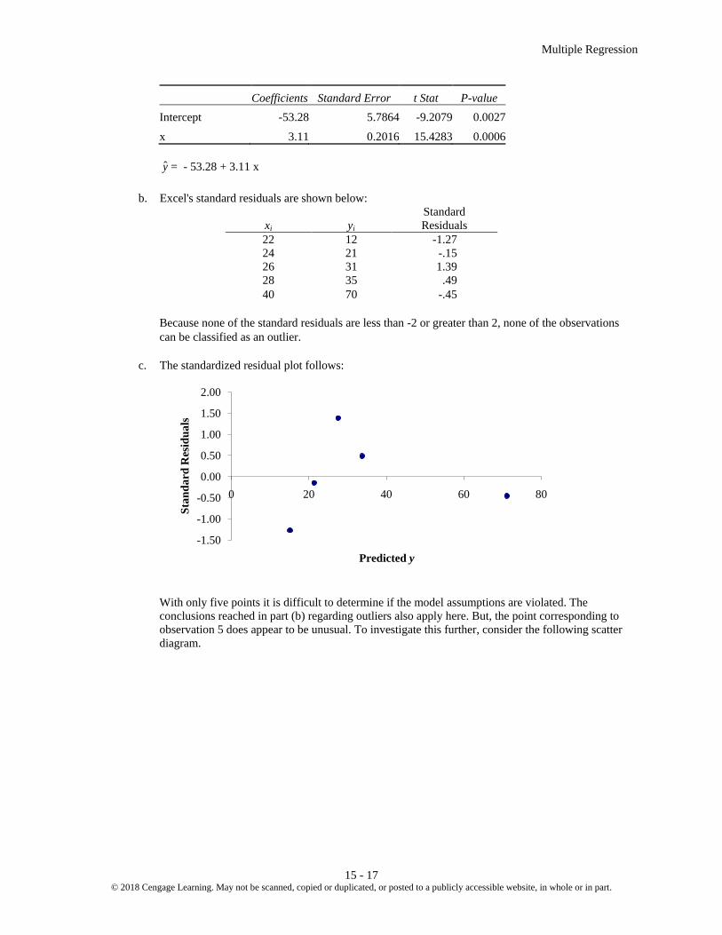
Multiple Regression
15 - 17 © 2018 Cengage Learning. May not be scanned, copied or duplicated, or posted to a publicly accessible website, in whole or in part.
Coefficients Standard Error t Stat P-value Intercept -53.28 5.7864 -9.2079 0.0027
x 3.11 0.2016 15.4283 0.0006 y = - 53.28 + 3.11 x b. Excel's standard residuals are shown below:
xi
yi
Standard Residuals
22 12 -1.27 24 21 -.15 26 31 1.39 28 35 .49 40 70 -.45
Because none of the standard residuals are less than -2 or greater than 2, none of the observations
can be classified as an outlier. c. The standardized residual plot follows:
With only five points it is difficult to determine if the model assumptions are violated. The conclusions reached in part (b) regarding outliers also apply here. But, the point corresponding to observation 5 does appear to be unusual. To investigate this further, consider the following scatter diagram.
-1.50
-1.00
-0.50
0.00
0.50
1.00
1.50
2.00
0 20 40 60 80
Stan
dard
Res
idua
ls
Predicted y

Chapter 15
15 - 18 © 2018 Cengage Learning. May not be scanned, copied or duplicated, or posted to a publicly accessible website, in whole or in part.
The scatter diagram indicates that observation 5 is influential.
42. a. Using datafile Auto2 and Excel’s Descriptive Statistics Regression Tool, the Excel output is shown
below:
Regression Statistics Multiple R 0.9588 R Square 0.9194 Adjusted R Square 0.9070 Standard Error 2.4853
Observations 16
ANOVA
df SS MS F Significance F Regression 2 915.6556134 457.8278 74.1202 7.79922E-08 Residual 13 80.2988 6.1768
Total 15 995.954375
Coefficients Standard Error t Stat P-value Intercept 71.3283 2.2479 31.7309 1.06E-13 Price ($1000s) 0.1072 0.0392 2.7355 0.0170
Horsepower 0.0845 0.0093 9.0801 5.45E-07 y = 71.3283+ 0.1072 Price + 0.0845 Horsepower b. The standardized residual plot is shown below. There appears to be a very unusual trend in the
residual plot. A different model should be considered.
01020304050607080
20 25 30 35 40 45
y
x

Multiple Regression
15 - 19 © 2018 Cengage Learning. May not be scanned, copied or duplicated, or posted to a publicly accessible website, in whole or in part.
c. The standardized residual plot did not identify any observations with a large standardized residual;
thus, there does not appear to be any outliers in the data. 44. a. The expected increase in final college grade point average corresponding to a one point increase in
high school grade point average is .0235 when SAT mathematics score does not change. Similarly, the expected increase in final college grade point average corresponding to a one point increase in the SAT mathematics score is .00486 when the high school grade point average does not change.
b. y = -1.41 + .0235(84) + .00486(540) = 3.1884 or about 3.19 46. a. The computer output with the missing values filled in is as follows:
Regression Statistics Multiple R 0.9607 R Square 0.923 Adjusted R Square 0.9102 Standard Error 3.35
Observations 15
ANOVA
df SS MS F Significance F Regression 2 1612 806 71.92 .0000 Residual 12 134.48 11.21
Total 14 1746.48
Coefficients Standard Error t Stat P-value Intercept 8.103 2.667 3.0382 0.0103 X1 7.602 2.105 3.6114 0.0036
X2 3.111 0.613 5.0750 0.0003 y = 8.103 + 7.602 X1 + 3.111 X2
-2.5-2
-1.5-1
-0.50
0.51
1.52
80 90 100 110 120
Stan
dard
Res
idua
ls
Predicted y

Chapter 15
15 - 20 © 2018 Cengage Learning. May not be scanned, copied or duplicated, or posted to a publicly accessible website, in whole or in part.
To start, we can calculate the Multiple R = r = 2r with the same sign as the slope. Therefore, r =
.923 .9607= Regression df = p = number of independent variables = 2 Regression df + Residual df = Total df = 2 + 12 = 14 Total df = n-1 =14 Therefore n=15 (number of observations)
2 2 1 15 11 (1 ) 1 (1 .923) .91021 15 2 1a
nR Rn p
− −= − − = − − =
− − − −
2 SSRSST
R = and therefore, 2
SSR 1612 1746.479.923
SSTR
= = =
SSE = SST - SSR = 1746.479 – 1612 = 34.479 MSR = SSR/p = 1612/2 = 806
SSE 1746.479MSE 11.2071 15 2 1n p
= = =− − − −
F = MSR/MSE = 806/11.207 = 71.92 Using Excel, the p-value = F.DIST.RT(71.92,2,12) = .0000
i
i
b
bt
s= and therefore, for the Intercept, 8.103 3.0382
2.667i
i
b
bt
s= = =
For the X1 coefficient, 7.602 3.61142.105
i
i
b
bt
s= = =
For the X2 coefficient, 3.111 5.0750.613
i
i
b
bt
s= = =
Degrees of freedom for the t tests for the coefficients = n – p - 1 = 12 Because t> 0, p-value is two times the upper tail area for each Using Excel: p-value for Intercept = 2*(1-T.DIST(3.0382,12,TRUE)) = .0103 Using Excel: p-value for X1 coefficient = 2*(1-T.DIST(3.6114,12,TRUE)) = .0036 Using Excel: p-value for X2 coefficient = 2*(1-T.DIST(5.0750,12,TRUE)) = .0003 b. The p-value (2 degrees of freedom numerator and 12 denominator) corresponding to F = 71.92 is
.0000 Because the p-value ≤ α = .05, there is a significant relationship. c. For β1: The p-value (12 degrees of freedom) corresponding to t = 3.6114 is .0036 Because the p-value ≤ α = .05, reject H0: β1 = 0 For β2 : The p-value (12 degrees of freedom) corresponding to t = 5.0750 is .0003 Because the p-value ≤ α = .05, reject H0: β2 = 0

Multiple Regression
15 - 21 © 2018 Cengage Learning. May not be scanned, copied or duplicated, or posted to a publicly accessible website, in whole or in part.
48. a. The regression equation is
Regression Statistics Multiple R 0.9493 R Square 0.9012 Adjusted R Square 0.8616 Standard Error 3.773 Observations 8 ANOVA
df SS MS F Significance F Regression 2 648.83 324.415 22.79 0.0031 Residual 5 71.17 14.2355 Total 7 720
Coefficients Standard Error t Stat P-value Intercept 14.4 8.191 1.7580 0.1391 X1 -8.69 1.555 -5.5884 0.0025 X2 13.517 2.085 6.4830 0.0013
y = 14.4 – 8.69 X1 + 13.517 X2 Standard error (top section) = 3.773 = MSEs =
Therefore, MSE = s2 = 3.7732 = 14.2355 = 71.17 71.1714.2355
1 2 1 3SSEMSE
n p n n= = = =
− − − − −
Using algebra, we can use this to solve for n (number of observations):
71.1714.2355
3n=
−and
71.173 514.2355
n − = = and therefore, n = 8
Regression df = p = number of independent variables = 2 Total df = n-1 =7 Residual df = Total df – Regression df = 7 – 2 = 5 Regression df + Residual df = Total df SSR = SST - SSE = 720 – 71.17 = 648.83
2 SSR 648.83 .90115SST 720
R = = =
2 2 1 8 11 (1 ) 1 (1 .90115) .86161 8 2 1a
nR Rn p
− −= − − = − − =
− − − −
Multiple R = r = 2r with the same sign as the slope. Therefore, r = .90115 .9493= MSR = SSR/p = 648.83/2 = 324.415 From earlier, s2 = MSE 14.2355=

Chapter 15
15 - 22 © 2018 Cengage Learning. May not be scanned, copied or duplicated, or posted to a publicly accessible website, in whole or in part.
F = MSR/MSE = 324.415/14.2355 = 22.79 Using Excel, the p-value = F.DIST.RT(22.79,2,5) = .0031
i
i
b
bt
s= and therefore, for the Intercept, 14.4 1.7580
8.191i
i
b
bt
s= = =
For the X1 coefficient, 8.69 5.58841.555
i
i
b
bt
s−
= = = −
For the X2 coefficient, 13.517 6.48302.085
i
i
b
bt
s= = =
Degrees of freedom for the t tests for the coefficients = n – p - 1 = 5 Because t< 0 for the X1 coefficient, p-value is two times the lower tail area Using Excel: p-value for X1 coefficient = 2*(T.DIST(-5.5884,5,TRUE)) = .0025 For the Intercept and X2 Coefficient, t> 0, p-value is two times the upper tail area for each Using Excel: p-value for Intercept = 2*(1-T.DIST(1.7580,5,TRUE)) = .1391 Using Excel: p-value for X2 coefficient = 2*(1-T.DIST(6.4830,5,TRUE)) = .0013 b. The p-value (2 degrees of freedom numerator and 5 degrees of freedom denominator) corresponding
to F = 22.79 is .0031 Because the p-value is ≤ α = .05, there is a significant relationship. c. 2 .9012R = 2 .8616aR = good fit d. For β1:the p-value (5 degrees of freedom) corresponding to t = -5.5884 is .0025. Because the p-value is ≤ α = .05, reject H0: β1 = 0 For β2: the p-value corresponding to t = 6.4830 is .0013 Because the p-value is ≤ α = .05, reject H0: β2 = 0
50. a. Using datafile 2012FuelEcon and Excel’s Descriptive Statistics Regression Tool, the Regression tool output follows.
Regression Statistics Multiple R 0.8013 R Square 0.6421 Adjusted R Square 0.6409 Standard Error 3.4123 Observations 309
ANOVA df SS MS F Significance F

Multiple Regression
15 - 23 © 2018 Cengage Learning. May not be scanned, copied or duplicated, or posted to a publicly accessible website, in whole or in part.
Regression 1 6413.2883 6413.2883 550.8029 1.79552E-70 Residual 307 3574.5628 11.6435
Total 308 9987.8511
Coefficients Standard Error t Stat P-value Intercept 41.0534 0.5166 79.4748 8.1E-207 Displacement -3.7232 0.1586 -23.4692 1.8E-70
y = 41.0534–3.7232Displacement
Because thep-value corresponding to F = 550.8029 is .0000 <α = .05, there is a significant
relationship. b. Using datafile 2012FuelEcon and Excel’s Descriptive Statistics Regression Tool, the Excel
Regression tool output follows.
Regression Statistics Multiple R 0.8276 R Square 0.6849 Adjusted R
Square 0.6829 Standard Error 3.2068 Observations 309
ANOVA
df SS MS F Significance
F Regression 2 6841.0876 3420.5438 332.6232 1.79466E-77 Residual 306 3146.7635 10.2835
Total 308 9987.8511
Coefficients Standard
Error t Stat P-value Intercept 40.5946 0.4906 82.7379 1.8E-211 Displacement -3.1944 0.1701 -18.7745 7.43E-53 FuelPremium -2.7230 0.4222 -6.4498 4.37E-10
y = 40.5946–3.1944Displacement ˗ 2.7230FuelPremium
c. For FuelPremium, the p-value corresponding to t = -6.4498 is .0000<α = .05; significant. The
addition of the dummy variables is significant. d. Using datafile 2012FuelEcon and Excel’s Descriptive Statistics Regression Tool, the Excel
Regression tool output follows.
Regression Statistics Multiple R 0.8554 R Square 0.7317 Adjusted R Square 0.7282 Standard Error 2.9688

Chapter 15
15 - 24 © 2018 Cengage Learning. May not be scanned, copied or duplicated, or posted to a publicly accessible website, in whole or in part.
Observations 309
ANOVA df SS MS F Significance F
Regression 4 7308.5436 1827.1359 207.3108 1.54798E-85 Residual 304 2679.3075 8.8135
Total 308 9987.8511
Coefficients
Standard Error t Stat P-value
Intercept 37.9626 0.7892 48.1055 3.5E-144 Displacement -3.2418 0.1941 -16.7007 6.97E-45 FuelPremium -2.1352 0.4519 -4.7253 3.52E-06 FrontWheel 3.0747 0.5394 5.7005 2.83E-08 RearWheel 3.3114 0.5413 6.1174 2.92E-09
y = 37.9626–3.2418Displacement–2.1352FuelPremium + 3.0747FrontWheel + 3.3114RearWheel
e. Since thep-value corresponding to F = 207.3108 is .0000<α= .05, there is a significant overall
relationship. Because the p-values for each independent variable are also <α= .05, each of the independent variables is significant.
52. a. Using datafileNBAStats and Excel’s Descriptive Statistics Regression Tool, the Excel output is
shown below:
Regression Statistics Multiple R 0.7339
R Square 0.5386 Adjusted R
Square 0.5221 Standard Error 10.7930 Observations 30
ANOVA df SS MS F Significance F
Regression 1 3807.7298 3807.7298 32.6876 3.92633E-06 Residual 28 3261.6772 116.4885
Total 29 7069.407
Coefficients Standard Error t Stat P-value Intercept -294.7669 60.3328 -4.8857 3.79099E-05
FG% 7.6966 1.3462 5.7173 3.92633E-06
y = –294.7669 + 7.6966 FG% Since the p-value corresponding to t = 5.7173 or F = 32.6876 is .000 <α = .05, there is a significant
relationship between the percentage of games won and the percentage of field goals made. b. An increase of 1% in the percentage of field goals made will increase the percentage of games won
by approximately 7.7%. c. Using datafileNBAStats and Excel’s Descriptive Statistics Regression Tool, the Excel output is shown
below:

Multiple Regression
15 - 25 © 2018 Cengage Learning. May not be scanned, copied or duplicated, or posted to a publicly accessible website, in whole or in part.
Regression Statistics
Multiple R 0.8764 R Square 0.7680 Adjusted R
Square 0.7197 Standard Error 8.2663 Observations 30
ANOVA df SS MS F Significance F
Regression 5 5429.4550 1085.8910 15.8916 6.13714E-07 Residual 24 1639.9520 68.3313
Total 29 7069.407
Coefficients Standard Error t Stat P-value Intercept -407.9703 68.9533 -5.9166 4.18419E-06
FG% 4.9612 1.3676 3.6276 0.0013 3P% 2.3749 0.8074 2.9413 0.0071 FT% 0.0049 0.5182 0.0095 0.9925 RBOff 3.4612 1.3462 2.5711 0.0168 RBDef 3.6853 1.2965 2.8425 0.0090 y = –407.9703 + 4.9612 FG% + 2.3749 3P% + 0.0049 FT% + 3.4612 RBOff + 3.6853 RBDef
d. For the estimated regression equation developed in part (c), the percentage of free throws made
(FT%) is not significant because the p-value corresponding to t = .0095 is .9925>α = .05. After removing this independent variable, using datafileNBAStats and Excel’s Descriptive Statistics Regression Tool, the Excel output is shown below:
Regression Statistics Multiple R 0.8764
R Square 0.7680 Adjusted R
Square 0.7309 Standard Error 8.0993 Observations 30
ANOVA df SS MS F Significance F
Regression 4 5429.4489 1357.3622 20.6920 1.24005E-07 Residual 25 1639.9581 65.5983
Total 29 7069.407
Coefficients Standard Error t Stat P-value Intercept -407.5790 54.2152 -7.5178 7.1603E-08
FG% 4.9621 1.3366 3.7125 0.0010 3P% 2.3736 0.7808 3.0401 0.0055 RBOff 3.4579 1.2765 2.7089 0.0120 RBDef 3.6859 1.2689 2.9048 0.0076

Chapter 15
15 - 26 © 2018 Cengage Learning. May not be scanned, copied or duplicated, or posted to a publicly accessible website, in whole or in part.
y = -407.5790 + 4.9621FG% + 2.3736 3P%+ 3.4579RBOff + 3.6859RBDef e. y = -407.5790 + 4.9621(45)+ 2.3736(35) + 3.4579(12) + 3.6859(30) = 50.9%