Chapter 1 VarietiesChapter 1 Varieties Outline: 1. Aﬃne varieties and examples. 2. The basics of...

Chapter 1

Varieties

Outline:

1. Affine varieties and examples.

2. The basics of the algebra-geometry dictionary.

3. Define Zariski topology (Zariski open and closed sets)

4. Primary decomposition and decomposition into components. Combinatorial defini-tion of dimension.

5. Regular functions. Complete the algebraic-geometric dictionary (equivalence of cat-egories). A whisper about schemes.

6. Rational functions.

7. Projective Varieties

8. Do projection and elimination. Use it to define the dimension of a variety. Provethe weak Nullstellensatz.

9. Appendix on Algebra.

1.1 Affine Varieties

The richness of algebraic geometry as a mathematical discipline comes from the interplayof algebra and geometry, as its basic objects are both geometrical and algebraic. The vividintuition of geometry is expressed with precision via the language of algebra. Symbolicand numeric manipulation of algebraic objects give practical tools for applications.

Let F be a field, which for us will be either the complex numbers C, the real numbersR, or the rational numbers Q. These different fields have their individual strengths andweaknesses. The complex numbers are algebraically closed; every univariate polnomial

1

2 CHAPTER 1. VARIETIES

has a complex root. Algebraic geometry works best when using an algebraically closedfield, and most introductory texts restrict themselves to the complex numbers. However,quite often real number answers are needed, particularly in applications. Because of this,we will often consider real varieties and work over R. Symbolic computation providesmany useful tools for algebraic geometry, but it requires a field such as Q, which can berepresented on a computer.

The set of all n-tuples (a1, . . . , an) of numbers in F is called affine n-space and writtenAn or An

Fwhen we want to indicate our field. We write An rather than Fn to emphasize

that we are not doing linear algebra. Let x1, . . . , xn be variables, which we regard ascoordinate functions on An and write F[x1, . . . , xn] for the ring of polynomials in thevariables x1, . . . , xn with coefficients in the field F. We may evaluate a polynomial f ∈F[x1, . . . , xn] at a point a ∈ An to get a number f(a) ∈ F, and so polynomials are alsofunctions on An. We make the main definition of this book.

Definition. An affine variety is the set of common zeroes of a collection of polynomials.Given a set S ⊂ F[x1, . . . , xn] of polynomials, the affine variety defined by S is the set

V(S) := {a ∈ An | f(a) = 0 for f ∈ S} .

This is a (affine) subvariety of An or simple a variety.

If X and Y are varieties with Y ⊂ X, then Y is a subvariety of X.The empty set ∅ = V(1) and affine space itself An = V(0) are varieties. Any linear

or affine subspace L of An is a variety. Indeed, L has an equation Ax = b, where A isa matrix and b is a vector, and so L = V(Ax − b) is defined by the linear polynomialswhich form the rows of Ax − b. An important special case of this is when L = {a} is apoint of An. Writing a = (a1, . . . , an), then L is defined by the equations xi − ai = 0 fori = 1, . . . , n.

Any finite subset Z ⊂ A1 is a variety as Z = V(f), where

f :=∏

z∈Z

(x− z)

is the monic polynomial with simple zeroes in Z.A non-constant polynomial p(x, y) in the variables x and y defines a plane curve

V(p) ⊂ A2. Here are the plane cubic curves V(p + 1

20), V(p), and V(p − 1

20), where

p(x, y) := y2 − x3 − x2.

1.1. AFFINE VARIETIES 3

The set of four points {(−2,−1), (−1, 1), (1,−1), (1, 2)} in A2 is a variety. It is theintersection of an ellipse V(x2+y2−xy−3) and a hyperbola V(3x2−y2−xy+2x+2y−3).

(−1, 1)

(1, 2)

(−2,−1) (1,−1)

V(3x2 − y2 − xy + 2x+ 2y − 3)

V(x2 + y2 − xy − 3)

A quadric is a variety defined by a single quadratic polynomial. In A2, these arethe plane conics (circles, ellipses, parabolas, and hyperbolas in R2) and in R3, these arethe spheres, ellipsoids, paraboloids, and hyperboloids. Figure 1.1 shows a hyperbolicparaboloid V(xy + z) and a hyperboloid of one sheet V(x2 − x+ y2 + yz).

x

y

z

V(xy + z)

x

y

z

V(x2 − x+ y2 + yz)

Figure 1.1: Two hyperboloids.

These last three examples, finite subsets of A1, plane curves, and quadrics, are varietiesdefined by a single polynomial and are called hypersurfaces. Any variety is an intersectionof hypersurfaces, one for each polynomial defining the variety.

The quadrics of Figure 1.1 meet in the variety V(xy + z, x2 − x + y2 + yz), whichis shown on the right in Figure 1.2. This intersection is the union of two space curves.One is the line x = 1, y + z = 0, while the other is the cubic space curve which hasparametrization (t2,−t, t3).

The intersection of the hyperboloid x2+(y− 3

2)2−z2 = 1

4with the sphere x2+y2+z2 = 4

is a single space curve (drawn on the sphere). If we instead intersect the hyperboloid withthe sphere centred at the origin having radius 1.9, then we obtain the space curve on the


x

y

z

x

y

z

Figure 1.2: Intersection of two quadrics.

right below.

The product V ×W of two varieties V and W is again a variety. Suppose that V ⊂ An

is defined by the polynomials f1, . . . , fs ∈ F[x1, . . . , xn] and the variety W ⊂ Am is definedby the polynomials g1, . . . , gt ∈ F[y1, . . . , ym]. Then X × Y ⊂ An×Am = An+m is definedby the polynomials f1, . . . , fs, g1, . . . , gt ∈ F[x1, . . . , xn, y1, . . . , ym].

The set Matn×n or Matn×n(F) of n×n matrices with entries in F is identified with theaffine space An2

. The special linear group is the set of matrices with determinant 1,

SLn := {M ∈ Matn×n | detM = 1} = V(det−1) .

We will show that SLn is smooth, irreducible, and has dimension n2 − 1. (We must first,of course, define these notions.)

We also point out some subsets of An which are not varieties. The set Z of integersis not a variety. The only polynomial vanishing at every integer is the zero polynomial,whose variety is all of A1. The same is true for any other infinite subset of A1, for example,the infinite sequence { 1

n| n = 1, 2, . . . } is not a subvariety of A1.

Other subsets which are not varieties (for the same reasons) include the unit disc in

1.2. THE ALGEBRA-GEOMETRY DICTIONARY I: IDEAL-VARIETY CORRESPONDENCE5

R2, {(x, y) ∈ R2 | x2 + y2 ≤ 1} or the complex numbers with positive real part.

x

y

unit disc�

��

1

1

−1

−1 R2

{z | Re(z) ≥ 0}�

−i

0

i

−1 1

C

Sets like these last two which are defined by inequalities involving real polynomials arecalled semi-algebraic. We will study them later.

1.2 The algebra-geometry dictionary I: ideal-variety

correspondence

We defined varieties V(S) associated to sets S ⊂ F[x1, . . . , xn] of polynomials,

V(S) = {a ∈ An | f(a) = 0 for all f ∈ S} .We would like to invert this association. Given a subset Z of An, consider the collectionof polynomials that vanish on Z,

I(Z) := {f ∈ F[x1, . . . , xn] | f(z) = 0 for all z ∈ Z} .The map I reverses inclusions so that Z ⊂ Y implies I(Z) ⊃ I(Y ).

These two inclusion-reversing maps

{Subsets S of F[x1, . . . , xn]}V−−→←−−I

{Subsets Z of An} (1.1)

form the basis of the algebra-geometry dictionary of affine algebraic geometry. We willrefine this correspondence to make it more precise.

An ideal is a subset I ⊂ F[x1, . . . , xn] which is closed under addition and undermuntiplication by polynomials in F[x1, . . . , xn]: If f, g ∈ I then f + g ∈ I and if wealso have h ∈ F[x1, . . . , xn], then hf ∈ I. The ideal 〈S〉 generated by a subset S ofF[x1, . . . , xn] is the smallest ideal containing S. This is the set of all expressions of theform

h1f1 + · · ·+ hmfm

where f1, . . . , fm ∈ S and h1, . . . , hm ∈ F[x1, . . . , xn]. We work with ideals because of f ,g, and h are polynomials and a ∈ An with f(a) = g(a) = 0, then (f + g)(a) = 0 and(hf)(a) = 0. Thus V(S) = V(〈S〉), and so we may restrict V to the ideals of F[x1, . . . , xn].In fact, we lose nothing if we restrict the left-hand-side of the correspondence (1.1) to theideals of F[x1, . . . , xn].


Lemma 1.2.1 For any subset S of An, I(S) is an ideal of F[x1, . . . , xn].

Proof. Let f, g ∈ I(S) be two polynomials which vanish at all points of S. Then f + gvanishes on S, as does hf , where h is any polynomial in F[x1, . . . , xn]. This shows thatI(S) is an ideal of F[x1, . . . , xn]. �

When S is infinite, the variety V(S) is defined by infinitely many polynomials. Hilbert’sbasis Theorem tells us that only finitely many of these polynomials are needed.

Hilbert’s Basis Theorem. Every ideal I of F[x1, . . . , xn] is finitely generated.

We defer the proof of this fundamental result until we discuss Grobner bases. Thisresult implies many important finiteness properties of algebraic varieties.†

Corollary 1.2.2 Any variety Z ⊂ An is the intersection of finitely many hypersurfaces.

Proof. Let Z = V(I) be defined by the ideal I. By Hilbert’s Basis Theorem, I is finitelygenerated, say by f1, . . . , fs, and so Z = V(f1, . . . , fs) = V(f1) ∩ · · · ∩ V(fs). �

Example. The ideal of the cubic space curve C of Figure 1.2 with parametrization(t2,−t, t3) not only contains the polynomials xy + z and x2 − x + y2 + yz, but alsoy2 − x, x2 + yz, and y3 + z. These polynomials are not all needed to define C asx2 − x + y2 + yz = (y2 − x) + (x2 + yz) and y3 + z = y(y2 − x) + (xy + z). In factthree of the quadrics suffice,

I(C) = 〈xy + z, y2 − x, x2 + yz〉 .

Lemma 1.2.3 For any subset Z of An, if X = V(I(Z)) is the variety defined by the ideal

I(Z), then I(X) = I(Z) and X is the smallest variety containing Z.

Proof. Set X := V(I(Z)). Then I(Z) ⊂ I(X), since if f vanishes on Z, it will vanishon X. However, Z ⊂ X, and so I(Z) ⊃ I(X), and thus I(Z) = I(X).

If Y was a variety with Z ⊂ Y ⊂ X, then I(X) ⊂ I(Y ) ⊂ I(Z) = I(X), and soI(Y ) = I(X). But then we must have Y = X for otherwise I(X) ( I(Y ), as is shown inExercise 6. �

Thus we also lose nothing if we restrict the right-hand-side of the correspondence (1.1)to the subvarieties of An. Our correspondence now becomes

{Ideals I of F[x1, . . . , xn]}V−−→←−−I

{Subvarieties X of An} (1.2)

This association is not a bijection. In particular, the map V is not one-to-one and themap I is not onto. There are several reasons for this.

†There, outline a proof of the usual (induction on the number of variables) proof in the exercises.


For example, when F = Q and n = 1, we have ∅ = V(1) = V(x2−2). The problem hereis that the rational numbers are not algebraically closed and we need to work with a largerfield (for example Q(

√2)) to study V(x2−2). When F = R and n = 1, ∅ 6= V(x2−2), but

we have ∅ = V(1) = V(1 + x2) = V(1 + x4). While the problem here is again that the realnumbers are not algebraically closed, we view this as a manifestation of positivity. Thetwo polynomials 1 + x2 and 1 + x4 only take positive values. When working over R (asour interest in applications leads us to) we will sometimes take positivity of polynomialsinto account.

The problem with the map V is more fundamental than these examples reveal andoccurs even when F = C. When n = 1 we have {0} = V(x) = V(x2), and when n = 2, weinvite the reader to check that V(y−x2) = V(y2−yx2, xy−x3). Note that while x 6∈ 〈x2〉,we have x2 ∈ 〈x2〉. Similarly, y − x2 6∈ V(y2 − yx2, xy − x3), but

(y − x2)2 = y2 − yx2 − x(xy − x3) ∈ 〈y2 − yx2, xy − x3〉 .

In both cases, the lack of injectivity of the map V boils down to f and fm having thesame set of zeroes, for any positive integer m. In particular, if f1, . . . , fs are polynomials,then the two ideals

〈f1, f2, . . . , fs〉 and 〈f1, f22 , f

33 , . . . , f

ss 〉

both define the same variety, and if fm ∈ I(Z), then f ∈ I(Z).We clarify this point with a definition. An ideal I ⊂ F[x1, . . . , xn] is radical if whenever

fm ∈ I for some m ≥ 1, then f ∈ I. The radical√I of an ideal I of F[x1, . . . , xn] is

defined to be√I := {f ∈ F[x1, . . . , xn] | fm ∈ I for some m ≥ 1} .

This turns out to be an ideal. In fact it is the smallest radical ideal containing I. Forexample, we just showed that

√

〈y2 − yx2, xy − x3〉 = 〈y − x2〉 .

The reason for this definition is twofold: I(Z) is radical and also an ideal and its radicalboth define the same variety. We record these facts.

Lemma 1.2.4 For Z ⊂ An, I(Z) is a radical ideal. If I ⊂ F[x1, . . . , xn] is an ideal, then

V(I) = V(√I).

When F is algebraically closed, the precise nature of the correspondence (1.2) fol-lows from Hilbert’s Nullstellensatz (null=zeroes, stelle=places, satz=theorem), another ofHilbert’s foundational results in the 1890’s† that helped to lay the foundations of algebraicgeometry and usher in twentieth century mathematics. We first state a weak form of theNullstellensatz, which describes the ideals defining the empty set.

†Likely his 1890 paper, maybe the 1893 one.


Theorem 1.2.5 (Weak Nullstellensatz) If I is an ideal of C[x1, . . . , xn] with V(I) =∅, then I = C[x1, . . . , xn].

Let a = (a1, . . . , an) ∈ An, which is defined by the linear polynomials xi − ai. Apolynomial f is equal to the constant f(a) modulo the ideal ma := 〈x1 − a1, . . . , xn − an〉generated by these polynomials, thus the quotient ring F[x1, . . . , xn]/ma is isomorphic tothe field F and so ma is a maximal ideal. In the appendix we show that when F = C (orany other algebraically closed field), these are the only maximal ideals.

Theorem 1.2.6 The maximal ideals of C[x1, . . . , xn] all have the form ma for some a ∈An.

Proof of Weak Nullstellensatz. We prove the contrapositive, if I ( C[x1, . . . , xn] is aproper ideal, then V(I) 6= ∅. There is a maximal ideal ma with a ∈ An of C[x1, . . . , xn]which contains I. But then

{a} = V(ma) ⊂ V(I) ,

and so V(I) 6= ∅. Thus if V(I) = ∅, we must have I = C[x1, . . . , xn], which proves theweak Nullstellensatz. �

We will later give a second proof that relies on geometric ideas.The Fundamental Theorem of Algebra states that any nonconstant polynomial f ∈

C[x] has a root (a solution to f(x) = 0). We recast the weak Nullstellensatz as themultivariate fundamental thoerem of algebra.

Theorem 1.2.7 (Multivariate Fundamental Theorem of Algebra) If the ideal gen-

erated by polynomials f1, . . . , fm ∈ C[x1, . . . , xn] is not the whole ring C[x1, . . . , xn], then

the system of polynomial equations

f1(x) = f2(x) = · · · = fm(x) = 0

has a solution in An.

We now deduce the full Nullstellensatz, which we will use to complete the characteri-zation (1.2).

Theorem 1.2.8 (Nullstellensatz) If I ⊂ C[x1, . . . , xn] is an ideal, then I(V(I)) =√I.

Proof. Since V(I) = V(√I), we have

√I ⊂ I(V(I)). We show the other inclusion.

Suppose that we have a polynomial f ∈ I(V(I)). Introduce a new variable t. Then thevariety V(tf−1, I) ⊂ An+1 defined by I and tf−1 is empty. Indeed, if (a1, . . . , an, b) werea point of this variety, then (a1, . . . , an) would be a point of V(I). But then f(a1, . . . , an) =0, and so the polynomial tf − 1 evaluates to 1 at the point (a1, . . . , an, b).


By the weak Nullstellensatz, 〈tf−1, I〉 = C[x1, . . . , xn, t]. In particular, 1 ∈ 〈tf−1, I〉,and so there exist polynomials f1, . . . , fm ∈ I and g, g1, . . . , gm ∈ C[x1, . . . , xn, t] such that

1 = g(x, t)(tf(x)− 1) + f1(x)g1(x, t) + f2(x)g2(x, t) + · · ·+ fm(x)gm(x, t) .

If we apply the substitution t = 1

f, then the first term with the factor tf − 1 vanishes and

each polynomial gi(x, t) becomes a rational function in x1, . . . , xn whose denominator is apower of f . Clearing these denominators gives an expression of the form

fN = f1(x)G1(x) + f2(x)G2(x) + · · ·+ fm(x)Gm(x) ,

where G1, . . . , Gm ∈ C[x1, . . . , xn]. But this shows that f ∈√I, and completes the proof

of the Nullstellensatz. �

Corollary 1.2.9 (Algebraic-Geometric Dictionary I) The maps V and I give an

inclusion reversing correspondence

{

Radical ideals Iof F[x1, . . . , xn]

}

V−−→←−−I

{Subvarieties X of An} (1.3)

with V(I(X)) = X. When F = C, the maps V and I are inverses, and this correspondence

is a bijection.

Proof. First, we already observed that I and V reverse inclusions and these maps havethe domain and range indicated. Let X be a subvariety of An. In Lemma 1.2.3 we showedthat X = V(I(X)). Thus V is onto and I is one-to-one.

Now suppose that F = C. By the Nullstellensatz, if I is radical then I(V(I)) = I,and so I is onto and V is one-to-one. In particular, this shows that I and V are inversebijections. �

Corollary 1.2.9 is only the beginning of the algebra-geometry dictionary. Many naturaloperations on varieties correspond to natural operations on their ideals. The sum I + Jand product I · J of ideals I and J are defined to be

I + J := {f + g | f ∈ I and g ∈ J}I · J := {f · g | f ∈ I and g ∈ J} .

Lemma 1.2.10 Let I, J be ideals in F[x1, . . . , xn] and set X := V(I) and Y = V(J) to

be their corresponding varieties. Then

1. V(I + J) = X ∩ Y ,

2. I(X ∩ Y ) =√I + J ,

3. V(I · J) = V(I ∩ J) = X ∪ Y , and


4. I(X ∪ Y ) =√I ∩ J =

√I · J .

Example. It can happen that I · J 6= I ∩ J . For example, if I = 〈xy − x3〉 and J =〈y2 − x2y〉, then I · J = 〈xy(y − x2)2〉, while I ∩ J = 〈xy(y − x2)〉.

This correspondence will be further refined in Section 1.5 to include maps betweenvarieties. Because of this correspondence, each geometric concept has a correspondingalgebraic concept, when F = C is algebraically closed. When F is not algebraically closed,this correspondence is not exact. In that case we will often use algebra to guide ourgeometric definitions.

Exercises for Section 1

1. Show that no proper nonempty open subset S of Rn or Cn is a variety. Here, wemean open in the usual (Euclidean) topology on Rn and Cn. (Hint: Consider theTaylor expansion of any polynomial in I(S).)

2. Verify the claim in the text that smallest ideal containing a set S ⊂ F[x1, . . . , xn] ofpolynomials is the set of all expressions of the form

h1f1 + · · ·+ hmfm

where f1, . . . , fm ∈ S and h1, . . . , hm ∈ F[x1, . . . , xn].

3. Prove that in A2, we have V(y − x2) = V(y3 − y2x2, x2y − x4).

4. Express the cubic space curve C with parametrization (t, t2, t3) in each of the fol-lowing ways.

(a) The intersection of a quadric and a cubic hypersurface.

(b) The intersection of two quadrics.

(c) The intersection of three quadrics.

5. Let I be an ideal of C[x1, . . . , xn]. Show that√I := {f ∈ F[x1, . . . , xn] | fm ∈ I for some m ≥ 1}

is an ideal, is radical, and is the smallest radical ideal containing I.

6. If Y ( X are varieties, show that I(X) ( I(Y ).

7. Suppose that I and J are radical ideals. Show that I ∩ J is also a radical ideal.

8. Give radical ideals I and J for which I + J is not radical.

9. Given ideals I and J show that {f · g | f ∈ I and g ∈ J} is an ideal.

1.3. GENERIC PROPERTIES OF VARIETIES 11

1.3 Generic properties of varieties

A useful feature in algebraic geometry is that many properties hold for almost all pointsof a variety or for almost all objects of a given type. For example, matrices are almostalways invertible, univariate polynomials of degree d almost always have d distinct roots,and multivariate polynomials are almost always irreducible. We develop the terminology‘generic’ and ‘Zariski open’ to describe this situation.

A starting point is that intersections and unions of affine varieties behave well.

Theorem 1.3.1 The intersection of any collection of affine varieties is an affine variety.

The union of any finite collection of affine varieties is an affine variety.

Proof. For the first statement, let {It | t ∈ T} be a collection of ideals in F[x1, . . . , xn].Then we have

⋂

t∈T

V(It) = V(

⋃

t∈T

It

)

.

Arguing by induction on the number of varieties, shows that it suffices to establish thesecond statement for the union of two varieties but that case is Lemma 1.2.10 (3). �

Theorem 1.3.1 shows that affine varieties have the same properties as the closed setsof a topology on An. This was observed by Oscar Zariski.

Definition. We call an affine variety a Zariski closed set. The complement of a Zariskiclosed set is a Zariski open set. The Zariski topology on An is the topology whose closedsets are the affine varieties in An. The Zariski closure of a subset Z ⊂ An is the smallestvariety containing Z, which is V(I(Z)), by Lemma 1.2.3. Any subvariety X of An inheritsits Zariski topology from An, the closed subsets are simply the subvarieties of X. A subsetZ ⊂ X of a variety X is Zariski dense in X if its closure is X.

We emphasize that the purpose of this terminology is to aid our discussion of varieties,and not because we will use notions from topology in any essential way. This Zariskitopology is behaves quite differently from the usual Euclidean topology on Rn or Cn withwhich we are familiar. A topology on a space may be defined by giving a collection of basicopen sets which generate the topology—any open set is a union or a finite intersection ofbasic open sets. In the Euclidean topology, the basic open sets are balls. The ball withradius ǫ > 0 centered at z ∈ Anis

B(z, ǫ) := {a ∈ An |∑

|ai − zi|2 < ǫ} .

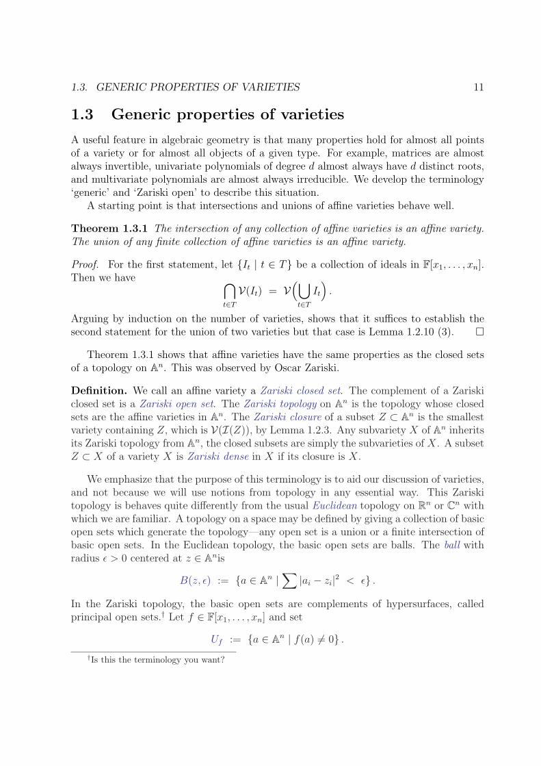
In the Zariski topology, the basic open sets are complements of hypersurfaces, calledprincipal open sets.† Let f ∈ F[x1, . . . , xn] and set

Uf := {a ∈ An | f(a) 6= 0} .†Is this the terminology you want?


In both these topologies the open sets are unions of basic open sets—we do not needintersections to generate the topology.

We give two examples to illustrate the Zariski topology.

Example. The Zariski closed subsets of A1 are the empty set, finite collections of points,and A1 itself. Thus when F is infinite the usual separation property of Hausdorff spaces(any two points are covered by two disjoint open sets) fails spectacularly as any twononempty open sets meet.

Example. The Zariski topology on a product X × Y of affine varieties X and Y is ingeneral not the product topology. In the product topology on A2, the closed sets are finiteunions of sets of the following form: the empty set, points, vertical and horizontal linesof the form {a} × A1 and A1 × {a}, and the whole space A2. On the other hand, A2

contains a rich collection of 1-dimensional subvarieties (called plane curves), such as thecubic plane curves of Section 1.1.

We compare the Zariski topology with the Euclidean topology.

Theorem 1.3.2 Suppose that F is one of R or C. Then

1. A Zariski closed set is closed in the Euclidean topology on An.

2. A Zariski open set is open in the Euclidean topology on An.

3. A nonempty Euclidean open set is Zariski dense.

4. Rn is Zariski dense in Cn.

5. A Zariski closed set is nowhere dense in the Euclidean topology on An.

6. A nonempty Zariski open set is dense in the the Euclidean topology on An.

Proof. For statements 1 and 2, observe that a Zariski closed set V(I) is the intersection ofthe hypersurfaces V(f) for f ∈ I, so it suffices to consider the case of a hypersurface V(f).But then Statement 1 (and hence also 2) follows as the polynomial function f : An → F

is continuous in the Euclidean topology, and V(f) = f−1(0).We show that any ball B(z, ǫ) is Zariski dense. If a polynomial f vanishes identically

on B(z, ǫ), then all of its partial derivaties do as well. This implies that its Taylor seriesexpansion at z is identically zero. But then f is the zero polynomial. This shows thatI(B) = {0}, and so V(I(B)) = An, that is, B is dense in the Zariski topology on An.

For statement 4, we use the same argument. If a polynomial vanishes on Rn, then allof its partial derivatives vanish and so f must be the zero polynomial. Thus I(Rn) = {0}and V(I(Rn)) = Cn.

For statements 5 and 6, observe that if f is nonconstant, then the interior of the(Euclidean) closed set V(f) is empty and so V(f) is nowhere dense. A subvariety isan intersection of nowhere dense hypersurfaces, so varieties are nowhere dense. Thecomplement of a nowhere dense set is dense, so Zariski open sets are dense in An. �

1.3. GENERIC PROPERTIES OF VARIETIES 13

The last statement of Theorem 1.3.2 leads to the important notions of genericity andgeneric sets and properties.

Definition. Let X be a variety. A subset Y ⊂ X is called generic if it contains a Zariskidense open subset of X. A property is generic if the set of points on which it holds is ageneric set. Points of a generic set are called general points.

This notion of general depends on the context, and so care must be exercised in itsuse. For example, the general quadratic polynomial ax2 + bx + c does not vanish whenx = 0. (We just need to avoid quadratics with c = 0.) On the other hand, the generalquadratic polynomial has two roots, as we need only avoid quadratics with b2 − 4ac = 0.The quadratic x2 − 2x + 1 is general in the first sense, but not in the second, while thequadratic x2+x is general in the second sense, but not in the first. Despite this ambiguity,we will see that this is a very useful concept.

When F is R or C, generic sets are dense in the Euclidean topology, by Theorem 1.3.2(6).Thus generic properties hold almost everywhere, in the standard sense.

Example. The generic n × n matrix is invertible, as it is a nonempty principal opensubset of Matn×n = An×n. It is the complement of the variety V(det) of singular matrices.Define the general linear group GLn to be the set of all invertible matrices,

GLn := {M ∈ Matn×n | det(M) 6= 0} = Udet .

Example. The general univariate polynomial of degree n has n distinct complex roots.Identify An with the set of univariate polynomials of degree n via

(a1, . . . , an) ∈ An 7−→ xn + a1xn−1 + · · ·+ an−1x+ an ∈ F[x] . (1.4)

The classical discriminant ∆ ∈ F[a1, . . . , an] is a polynomial of degree 2n − 1 whichvanishes precisely when the polynomial (1.4) has a repeated factor. This identifies the setof polynomials with n distinct complex roots as the set U∆. The discriminant of a quadricx2 + bx+ c is b2 − 4c.

Example. The generic complex n × n matrix is semisimple (diagonalizable). Let M ∈Matn×n and consider the (monic) characteristic polynomial of M

χ(x) := det(xIn −M) .

We do not show this by providing an algebraic characterization of semisimplicity. Insteadwe observe that if a matrix M ∈ Matn×n has n distinct eigenvalues, then it is semisimple.The coefficients of the characteristic polynomial χ(x) are polynomials in the entries ofM . Evaluating the discriminant at these coefficients gives a polynomial ψ which vanisheswhen the characteristic polynomial χ(x) of M has a repeated root.


We see that the set of matrices with distinct eigenvalues equals the basic open set Uψ,which is nonempty. Thus the set of semisimple matrices contains an open dense subset ofMatn×n set and is therefore generic.

When n = 2,

det

(

xI2 −[

a11 a12

a21 a22

])

= t2 − t(a11 + a22) + a11a22 − a12a21 ,

and so the polynomial ψ is (a11 + a22)2 − 4(a11a22 − a12a21) .

In each of these examples, we used the following easy fact.

Proposition 1.3.3 A set X ⊂ An is generic if and only if there is a nonconstant poly-

nomial that vanishes on its complement.

Exercises

1. Look up the definition of a topology in a text book and verify the claim that thecollection of affine subvarieties of An form the closed sets in a topology on An.

2. Prove that a closed set in the Zariski topology on A1 is either the empty set, a finitecollection of points, or A1 itself.

3. Let n ≤ m. Prove that a generic n×m matrix has rank n.

4. Prove that the generic triple of points in A2 are the vertices of a triangle.

1.4. UNIQUE FACTORIZATION FOR VARIETIES 15

1.4 Unique factorization for varieties

We establish a basic structure theorem for affine varieties which is an analog of uniquefactorization for polynomials. A polynomial f ∈ F[x1, . . . , xn] is reducible if we may factorf notrivially, that is, if f = gh with neither g nor h a constant polynomial. Otherwise fis irreducible. Any polynomial f ∈ F[x1, . . . , xn] may be factored

f = gα1

1 gα2

2 · · · gαm

m (1.5)

where the exponents αi are positive integers, each polynomial gi is irreducible and non-constant, and when i 6= j the polynomials gi and gj are not proportional. This fac-torization is essentially unique as any other such factorization is obtained from this bypermuting the factors and possibly multiplying each polynomial gi by a constant. Thepolynomials gj are irreducible factors of f .

This algebraic property has a consequence for the geometry of hypersurfaces. Supposethat a polynomial f is factored into irreducibles (1.5). Then the hypersurface X = V(f)is the union of hypersurfaces Xi := V(gi), and this decomposition

X = X1 ∪X2 ∪ · · · ∪Xm

of X into hypersurfaces Xi defined by irreducible polynomials is unique.This decomposition property is shared by general affine varieties.

Definition. An affine variety X is reducible if it is the union X = Y ∪Z of proper closedsubvarieties Y, Z ( X. Otherwise X is irreducible. In particular, if an irreducible varietyis written as a union of subvarieties X = Y ∪ Z, then either X = Y or X = Z.

Example. Figure 1.2 shows that the variety V(xy + z, x2 − x+ y2 + yz) consists of twospace curves, each of which is a variety in its own right. Thus it is reducible. To see this,we solve the two equations xy + z = x2 − x+ y2 + yz = 0. First note that

x2 − x+ y2 + yz − y(xy + z) = x2 − x+ y2 − xy2 = (x− 1)(x− y2) .

Thus either x = 1 or else x = y2. When x = 1, we see that y+ z = 0 and these equationsdefine the line in Figure 1.2. When x = y2, we get z = y3, and these equations define thecubic curve parametrized by (t2, t, t3).

Here is another reducible variety. It has three components, one is a surface and theother two are curves.


Theorem 1.4.1 A product X × Y of irreducible varieties is irreducible.

Proof. Suppose that Z1, Z2 ⊂ X ×Y are subvarieties with Z1 ∪Z2 = X ×Y . We assumethat Z2 6= X × Y and use this to show that Z1 = X × Y . For each x ∈ X, identify thesubvariety {x} × Y with Y . This irreducible variety is the union of two subvarieties,

{x} × Y =(

({x} × Y ) ∩ Z1

)

∪(

({x} × Y ) ∩ Z2

)

,

and so one of these must equal {x}×Y . In particular, we must either have {x}×Y ⊂ Z1

or else {x} × Y ⊂ Z2. If we define

X1 = {x ∈ X | {x} × Y ⊂ Z1} , and

X2 = {x ∈ X | {x} × Y ⊂ Z2} ,

then we have just shown that X = X1 ∪ X2. Since Z2 6= X × Y , we have X2 6= X. Weclaim that both X1 and X2 are subvarieties of X. Then the irreducibility of X impliesthat X = X1 and thus X × Y = Z1.

We will show that X1 is a subvariety of X. For y ∈ Y , set

Xy := {x ∈ X | (x, y) ∈ Z1} .

Since Xy × {y} = (X × {y}) ∩ Z1, we see that Xy is a subvariety of X. But we have

X1 =⋂

y∈Y

Xy ,

which shows that X1 is a subvariety of X. An identical argument for X2 completes theproof. �

The geometric notion of an irreducible variety corresponds to the algebraic notion ofa prime ideal. An ideal I ⊂ F[x1, . . . , xn] is prime if whenever fg ∈ I with f 6∈ I, then wehave g ∈ I. Equivalently, if whenever f, g 6∈ I then fg 6∈ I.

Theorem 1.4.2 An affine variety X is irredicuble if and only if its ideal I(X) is prime.

Proof. Let X be an affine variety and set I := I(X). First suppose that X is irreducible.Let f, g 6∈ I. Then neither f nor g vanishes identically on X. Thus Y := X ∩ V(f) andZ := X ∩ V(z) are proper subvarieties of X. Since X is irreducible, Y ∪ Z = X ∩ V(fg)is also a proper subvariety of X, and thus fg 6∈ I.

Suppose now that X is reducible. Then X = Y ∪Z is the union of proper subvarietiesY, Z of X. Since Y ( X is a subvariety, we have I(X) ( I(Y ). Let f ∈ I(Y ) − I(X),a polynomial which vanishes on Y but not on X. Similarly, let g ∈ I(Z) − I(X) be apolynomial which vanishes on Z but not on X. Since X = Y ∪ Z, fg vanishes on X andtherfore lies in I(X). This shows that I is not prime. �


We have seen examples of varieties with one, two, and three irreducible components.Taking products of distinct irreducible polynomials (or dually unions of distinct hyper-surfaces), gives varieties having any finite number of irreducible components. This is allcan occur as Hilbert’s Basis Theorem implies that a variety is a union of finitely manyirreducible varieties.

Lemma 1.4.3 Any affine variety is a finite union of irreducible subvarieties.

Proof. An affine variety X either is irreducible or else we have X = Y ∪ Z, with bothY and Z proper subvarieties of X. We may similarly decompose whichever of Y and Zare reducible, and continue this process, stopping only when all subvarieties obtained areirreducible. A priori, this process could continue indefinitely. We argue that it must stopafter a finite number of steps.

If this process never stops, then X must contain an infinite chain of subvarieties, eachone properly contained in the previous one,

X ) X1 ) X2 ) · · · .

Their ideals form an infinite increasing chain of ideals in F[x1, . . . , xn],

I(X) ( I(X1) ( I(X2) ( · · · .

The union I of these ideals is again an ideal. Note that no ideal I(Xm) is equal to I. Bythe Hilbert Basis Theorem, I is finitely generated, and thus there is some integer m forwhich I(Xm) contains these generators. But then I = I(Xm), a contradiction. �

A consequence of this proof is that any decreasing chain of subvarieties of a givenvariety must have finite length. There is however a bound for the length of the longestdecreasing chain of irreducible subvarieties.

Combinatorial Definition of Dimension. The dimension of an irreducible variety Xis given by the length of the longest decreasing chain of irreducible subvarieties of X. If

X ⊂ X0 ) X1 ) X2 ) · · · ) Xm ) ∅ ,

is such a chain of maximal length, then X has dimension m.

Since maximal ideals of C[x1, . . . , xn] necessarily have the form ma, we see that Xm

must be a point when F = C. The only problem with this definition is that we cannot yetshow that it is well-founded, as we do not yet know that there is a bound on the lengthof such a chain. Later we shall prove that this definition is correct by relating it to othernotions of dimension.


Example. The sphere S has dimenion at least two, as we have the chain of subvarietiesS ) C ) P as shown below.

SHHHj

C -

P�

It is quite challenging to show that any maximal chain of irreducble subvarieties of thesphere has length 2 with the tools that we have developed.

By Lemma 1.4.3, an affine variety X may be written as a finite union

X = X1 ∪ X2 ∪ · · · ∪ Xm

of irreducible subvarieties. We may assume that this is irredundant in that if i 6= j thenXi is not a subvariety of Xj. If we did have i 6= j with Xi ⊂ Xj, then we may remove Xi

from the decomposition. We prove that this decomposition is unique, which is the mainresult of this section and a basic structural result about varieties.

Theorem 1.4.4 (Unique Decomposition of Varieites) An affine variety X has a unique

irredundant decomposition as a finite union of irreducible subvarieties

X = X1 ∪ X2 ∪ · · · ∪ Xm .

We call these distinguished subvarieties Xi the irreducible components of X.

Proof. Suppose that we have another irredundant decomposition into irreducible subva-rieties,

X = Y1 ∪ Y2 ∪ · · · ∪ Yn ,

where each Yi is irreducible. Then

Xi = (Xi ∩ Y1) ∪ (Xi ∩ Y2) ∪ · · · ∪ (Xi ∩ Yn) .

Since Xi is irreducible, one of these must equal Xi, which means that there is some indexj with Xi ⊂ Yj. Similarly, there is some index k with Yj ⊂ Xk. Since this implies thatXi ⊂ Xk, we have i = k, and so Xi = Yj. This implies that n = m and that the seconddecomposition differs from the first solely by permuting the terms. �


When F = C, we will show that an irreducible variety is connected in the ususalEuclidean topology.† We will even show that the smooth points of an irreducible varietyare connected. Neither of these facts are true over R. Below, we display the irreduciblecubic plane curve V(y2−x3 +x) in A2

Rand the surface V((x2−y2)2−2x2−2y2−16z2 +1)

in A3R.

Both are irreducible hypersurfaces. The first has two connected components in the Eu-clidean topology, while in the second, the five components of singular points meet at thefour singular points.

Exercises

1. Show that the ideal of a hypersurface V(f) is generated by the squarefree part of f ,which is the product of the irreducible factors of f , all with exponent 1.

2. For every positive integer n, give a decreasing chain of subvarieties of A1 of lengthn+1.

3. Prove that the dimension of a point is 0 and the dimension of A1 is 1.

4. Prove that the dimension of an irreducible plane curve is 1 and use this to showthat the dimension of A2 is 2.

5. Write the ideal 〈x3 − x, x2 − y〉 as the intersection of two prime ideals. Decribe thecorreponding geometry.

†When and where will we show this?


1.5 The algebra-geometry dictionary II

The algebra-geometry dictionary of Section 1.2 is strengthened when we include regularmaps between varieties and the corresponding homomorphisms between rings of regularfunctions.

Let X ⊂ An be an affine variety. Any polynomial function f ∈ F[x1, . . . , xn] restrictsto give a regular function on X, f : X → F. We may add and multiply regular functions,and the set of all regular functions on X forms a ring, F[X], called the coordinate ring

of the affine variety X or the ring of regular functions on X. The coordinate ring of anaffine variety X is a basic invariant of X, which is, in fact equivalent to X itself.

The restriction of polynomial functions on An to regular functions on X defines asurjective ring homomorphism F[x1, . . . , xn] ։ F[X]. The kernel of this restriction ho-momorphism is the set of polynomials which vanish identically on X, that is, the idealI(X) of X. Under the correspondence between ideals, quotient rings, and homomor-phisms, this restriction map gives and isomorphism between F[X] and the quotient ringF[x1, . . . , xn]/I(X).

Example. The coordinate ring of the parabola y = x2 is F[x, y]/〈y − x2〉, which is iso-morphic to F[x], the coordinate ring of A1. To see thia, observe that substituting x2 fory rewrites and polynomial f(x, y) as a polynomial g(x) in x alone, and y− x2 divides thedifference f(x, y)− g(x).

On the other hand, the coordinate ring of the semicubical parabola y2 = x3 isF[x, y]/〈y2 − x3〉. This ring is not isomorphic to the previous ring. For example, theelement y2 = x3 has two factorizations into irreducible elements, while polynomials F[x]in one variable always factor uniquely

Parabola Semicubical Parabola

This quotient ring F[x1, . . . , xn]/I(X) is finitely generated by the images of the vari-ables xi. Since I(X) is radical, the quotient ring has no nilpotent elements (elements fsuch that fm = 0 for some m) and is therefore reduced. When F is algebraically closed,these two properties characterize coordinate rings of algebraic varieties.

Theorem 1.5.1 Suppose that F is algebraically closed. Then an F algebra R is the coor-

dinate ring of an affine variety if and only if R is finitely generated and reduced.

Proof. We need only show that a finitely generated reduced F algebra R is the coordinatering of an affine variety. Suppose that the reduced F algebra R has generators r1, . . . , rn.Then there is a surjective ring homomorphism

ϕ : F[x1, . . . , xn] −։ R

1.5. THE ALGEBRA-GEOMETRY DICTIONARY II 21

given by xi 7→ ri. Let I ⊂ F[x1, . . . , xn] be the kernel of ϕ. This identifies R withF[x1, . . . , xn]/I. Since R is reduced, we see that I is radical.

When F is algebraically closed, the algebra-geometry dictionary of Corollary 1.2.9shows that I = I(V(I)) and so R ≃ F[x1, . . . , xn]/I ≃ F[V(I)]. �

A different choice s1, . . . , sm of generators for R in this proof will give a different affinevariety with coordinate ring R. One goal of this section is to understand this apparentambiguity.

Example. Consider the finitely generated F algebra R := F[t]. Chosing the generator trealizes R as F[A1]. We could, however choose as generators x := t + 1 and y := t2 + 3t.Since y = x2 +x−2, this also realizes R as F[x, y]/〈y−x2−x+2〉, which is the coordinatering of a parabola.

Among the coordinate rings F[X] of affine varieties are the polynomial algebras F[An] =F[x1, . . . , xn]. Many properties of polynomial algebras, including the algebra-geometry ofCorollary 1.2.9 and the Hilbert Theorems hold for these coordinate ring F[X].

Given regular functions f1, . . . , fm ∈ F[X] on an affine variety X ⊂ An, their set ofcommon zeroes

V(f1, . . . , fm) := {x ∈ X | f1(x) = · · · = fm(x) = 0} ,

is a subvariety of X. Indeed, let F1, . . . , Fm ∈ F[x1, . . . , xn] be polynomials which restrictto f1, . . . , fm. Then

V(f1, . . . , fm) = X ∩ V(F1, . . . , Fm) .

As in Section 1.2, we may extend this notation and define V(I) for an ideal I of F[X].If Y ⊂ X is a subvariety of X, then I(X) ⊂ I(Y ) and so I(Y )/I(X) is an ideal in thecoordinate ring F[X] = F[An]/I(X) of X. Write I(Y ) ⊂ F[X] for the ideal of Y in F[X].

Both Hilbert’s Basis Theorem and Hilbert’s Nulstellensatz have analogs for affinevarieties X and their coordinate rings F[X]. These consequences of the original HilbertTheorems follow from the surjection F[x1, . . . , xn] ։ F[X] and corresponding inclusionX → An.

Theorem 1.5.2 (Hilbert Theorems for F[X]) Let X be an affine variety. Then

1. Any ideal of F[X] is finitely generated.

2. If Y is a subvariety of X then I(Y ) ⊂ F[X] is a radical ideal. The subvariety Y is

irreducible if and only if I(Y ) is a prime ideal.

3. Suppose that F is algebraically closed. An ideal I of F[X] defines the empty set if

and only if I = F[X].


In the same way as in Section 1.2 we obtain a version of the algebra-geometry dictionarybetween subvarieties of an affine variety X and radical ideals of F[X]. The proofs are thesame, so we leave them to the reader. For this, you will need to recall that ideals J of aquotient ring R/I all have the form K/I, where K is an ideal of R which contains I.

Theorem 1.5.3 Let X be an affine variety. Then the maps V and I give an inclusion

reversing correspondence

{Radical ideals I of F[X]}V−−→←−−I

{Subvarieties Y of X} (1.6)

with I injective and V surjective. When F = C, the maps V and I are inverses, and this

correspondence is a bijection.

In algebraic geometry, we do not just study varieties, but also the maps between them.

Definition. A list f1, . . . , fm ∈ F[X] of regular functions on an affine variety X definesa function

ϕ : X −→ Am

x 7−→ (f1(x), f2(x), . . . , fm(x)) ,

which we call a regular map.

Example. The elements t2, t, t3 ∈ F[t] = F[A1] define the map A1 → A3 with image thecubic curve of Figure 1.1.

The elements t2, t3 of F[A1] define a map A1 → A2 whose image is the cuspidal cubicthat we saw earlier.

Let x = t2 − 1 and y = t3 − t, which are elements of F[t] = F[A1]. These define a mapA1 → A2 whose image is the cubic curve V(y2− (x3 +x2)) on the left below. If we insteadtake x = t2 + 1 and y = t3 + t, then we get a different map A1 → A2 whose image is thecurve on the right below.

In the curve on the right, the image of A1R

is the arc, while the isolated or solitary point

is the image of the points ±√−1.

Suppose that X is an affine variety and we have a regular map ϕ : X → Am given byregular functions f1, . . . , fm ∈ F[X]. A polynomial g ∈ F[x1, . . . , xm] ∈ F[Am] pulls back

along ϕ to give the regular function ϕ∗g, which is defined by

ϕ∗g := g(f1, . . . , fm) .

1.5. THE ALGEBRA-GEOMETRY DICTIONARY II 23

This is an element of the coordinate ring F[X] of X. This is the usual pull back of afunction, for x ∈ X,

ϕ∗g(x) = g(ϕ(x)) = g(f1(x), . . . , fm(x)) .

The resulting map ϕ∗ : F[Am] → F[X] is a homomorphism of F algebras. Conversely,given a homomorphism ψ : F[x1, . . . , xm]→ F[X] of F algebras, if we set fi := ψ(xi), thenf1, . . . , fm ∈ F[X] define a regular map ϕ with ϕ∗ = ψ.

We have just shown the following basic fact.

Lemma 1.5.4 The association ϕ 7→ ϕ∗ defines a bijection

{

regular maps

ϕ : X → Am

}

←→{

ring homomorphisms

ψ : F[Am]→ F[X]

}

In the examples that we gave, the image ϕ(X) of X under ϕ was contained in asubvariety. This is always the case.

Lemma 1.5.5 Let X be an affine variety, ϕ : X → Am a regular map, and Y ⊂ Am a

subvariety. Then ϕ(X) ⊂ Y if and only if I(Y ) ⊂ kerϕ∗.

Proof. Suppose that ϕ(X) ⊂ Y . If f ∈ I(Y ) then f vanishes on Y and hence on ϕ(X).But then ϕ∗f is the zero function. Thus I(Y ) ⊂ kerϕ∗.

For the other direction, suppose that I(Y ) ⊂ kerϕ∗ and let x ∈ X. If f ∈ I(Y ), thenϕ∗f = 0 and so 0 = ϕ∗f(x) = f(ϕ(x)). Since this is true for every f ∈ I(Y ), we concludethat ϕ(x) ∈ Y . Since this is true for every x ∈ X, we conclude that ϕ(X) ⊂ Y . �

Corollary 1.5.6 Let X be an affine variety, ϕ : X → Am a regular map, and Y ⊂ Am a

subvariety. Then

(1) kerϕ∗ is a radical ideal.

(2) If X is irreducible, then kerϕ∗ is a prime ideal.

(3) V(kerϕ∗) is the smallest affine variety containing ϕ(X).

(4) If ϕ : X → Y , then ϕ∗ : F[Y ]→ F[X].

Proof. For (1), suppose that fm ∈ kerϕ∗, so that 0 = ϕ∗(fm) = (ϕ(f))m. Since F[X]has no nilpotent elements, we conclude that ϕ(f) = 0 and so f ∈ kerϕ∗.†

For (2), suppose that f ·g ∈ kerϕ∗ with g 6∈ kerϕ∗. Then 0 = ϕ∗(f ·g) = ϕ∗(f)·ϕ∗(g) inF[X], but 0 6= ϕ∗(g). Since F[X] is a domain, we must have 0 = ϕ∗(f) and so f ∈ kerϕ∗,which shows that kerϕ∗ is a prime ideal.

†Mabe we should do these in the Appendix and just quote them from there.


Suppose that Y is an affine variety containing ϕ(X). By Lemma 1.5.5 I(Y ) ⊂ kerϕ∗

and so V(kerϕ∗) ⊂ Y . Statement (3) follows as we also have X ⊂ V(kerϕ∗).For (4), we have I(Y ) ⊂ kerϕ∗ and so the map ϕ∗ : F[A1]→ F[X] factors through the

quotient map F[A1] ։ F[A1]/I(Y ). reword this better! Maybe do this last one in the text?

�

Thus we may refine the correspondence of Lemma 1.5.4. Let X and Y be affinevarieties. Then ϕ 7→ ϕ∗ gives a bijective correspondence

{

regularmapsϕ : X → Y

}

←→{

ring homomorphismsψ : F[Y ]→ F[X]

}

This map X 7→ F[X] from affine varieties to finitely generated F algebras withoutnilpotents not only maps objects to objects, but is an isomorphism on maps betweenobjects. In mathematics, such an association is called a contravariant equivalence of

categories.The prototypical example of this comes from linear algebra. To a finite-dimensional

vector space V , we may associate its dual space V ∗. Given a linear transformation L : V →W , its adjoint is a map L∗ : W ∗ → V ∗. Since (V ∗)∗ = V and (L∗)∗ = L, this associationis a bijection on the objects (finite-dimensional vector spaces) and a bijection on linearmaps linear maps from V to W .

Need to discuss more about the equivalence of categories, and then make a whisper about

schemes.

1. Give a proof of Theorem 1.5.2.

2. Show that a regular map ϕ : X → Y is continuous in the Zariski topology.

1.6 Rational functions

1.7 Smooth and singular points

1.8 Projective varieties

Notes

At the end of chapters, we should have a section on notes which describes some of the his-tory, etc. In this chapter, we need only discuss some other sources for Algebraic Geometryand maybe Hilbert’s breakthroughs.

Chapter 1 VarietiesChapter 1 Varieties Outline: 1. Aﬃne varieties and examples. 2. The basics of...

Documents

Transcript of Chapter 1 VarietiesChapter 1 Varieties Outline: 1. Aﬃne varieties and examples. 2. The basics of...