Chapter 1

An Introduction to Model Building

to accompany

Operations Research: Applications and Algorithms

4th edition

by Wayne L. Winston

Copyright (c) 2004 Brooks/Cole, a division of Thomson Learning, Inc.

2

1.1 An Introduction to Modeling

Operations research (management science) is a scientific approach to decision making that seeks to best design and operate a system, usually under conditions requiring the allocation of scarce resources.

Term coined during WW II when leaders asked scientists and engineers to analyze several military problems.

A system is an organization of interdependent components that work together to accomplish the goal of the system.

3

The scientific approach to decision making requires the use of one or more mathematical models.

A mathematical model is a mathematical representation of the actual situation that may be used to make better decisions or clarify the situation.

4

Example 1: A Modeling Example

Eli Daisy produces the drug Wozac in batches by heating a chemical mixture in a pressurized container.

Each time a batch is produced, a different amount of Wozac is produced.

The amount produced is the process yield (measured in pounds).

Daisy is interested in understanding the factors that influence the yield of Wozac production process.

Describe a model-building process for this situation.

5

Example 1: Solution

Daisy is first interested in determining the factors that influence the process yield.

This is a descriptive model since it describes the behavior of the actual yield as a function of various factors.

Daisy might determine that the following factors influence yield:

Container volume in liters (V)

Container pressure in milliliters (P)

Container temperature in degrees centigrade (T)

Chemical composition of the processed mixture

6

Ex. 1: Solution continued

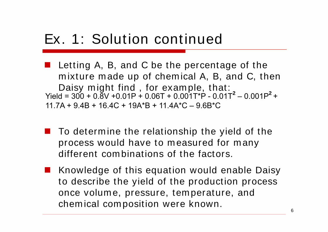
Letting A, B, and C be the percentage of the mixture made up of chemical A, B, and C, then Daisy might find , for example, that:

To determine the relationship the yield of the process would have to measured for many different combinations of the factors.

Knowledge of this equation would enable Daisy to describe the yield of the production process once volume, pressure, temperature, and chemical composition were known.

Yield = 300 + 0.8V +0.01P + 0.06T + 0.001T*P - 0.01T2 – 0.001P2 + 11.7A + 9.4B + 16.4C + 19A*B + 11.4A*C – 9.6B*C

7

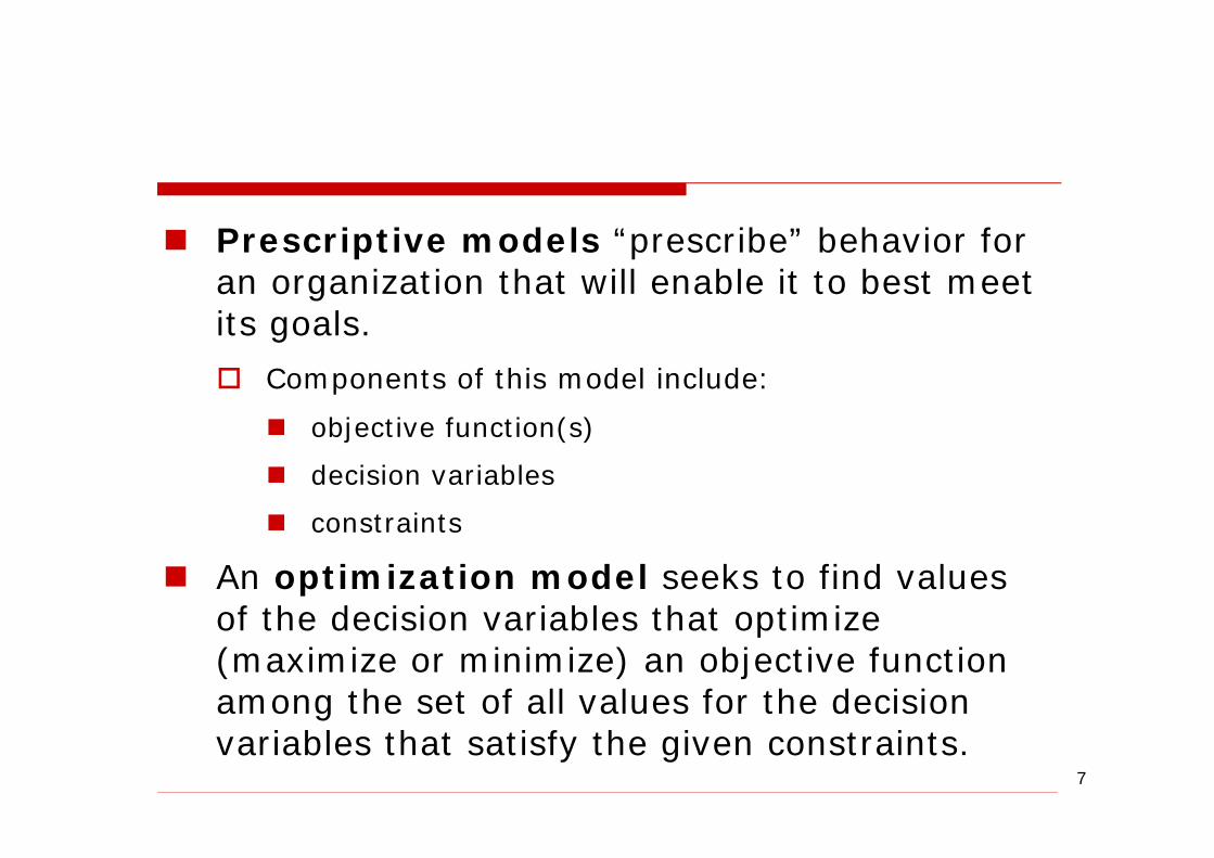
Prescriptive models “prescribe” behavior for an organization that will enable it to best meet its goals.

Components of this model include:

objective function(s)

decision variables

constraints

An optimization model seeks to find values of the decision variables that optimize (maximize or minimize) an objective function among the set of all values for the decision variables that satisfy the given constraints.

8

Ex. 1: Solution continued

The Daisy example seeks to maximize the yield for the production process.

In most models, there will be a function we wish to maximize or minimize. This function is called the model’s objective function.

To maximize the process yield we need to find the values of V, P, T, A, B, and C that make the yield equation (below) as large as possible.

Yield = 300 + 0.8V +0.01P + 0.06T + 0.001T*P - 0.01T2 – 0.001P2

+ 11.7A + 9.4B + 16.4C + 19A*B + 11.4A*C – 9.6B*C

9

In many situations, an organization may have more than one objective.

For example, in assigning students to the two high schools in Bloomington, Indiana, the Monroe County School Board stated that the assignment of students involve the following objectives:

equalize the number of students at the two high schools

minimize the average distance students travel to school

have a diverse student body at both high schools

10

Variables whose values are under our control and influence system performance are called decision variables.

In the Daisy example, V, P, T, A, B, and C are decision variables.

In most situations, only certain values of the decision variables are possible.

For example, certain volume, pressure, and temperature conditions might be unsafe. Also, A, B, and C must be nonnegative numbers that sum to one.

These restrictions on the decision variable values are called constraints.

11

Ex. 1: Solution continued

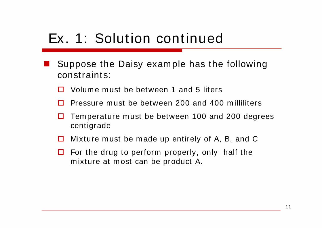
Suppose the Daisy example has the following constraints:

Volume must be between 1 and 5 liters

Pressure must be between 200 and 400 milliliters

Temperature must be between 100 and 200 degrees centigrade

Mixture must be made up entirely of A, B, and C

For the drug to perform properly, only half the mixture at most can be product A.

12

Ex. 1: Solution continued

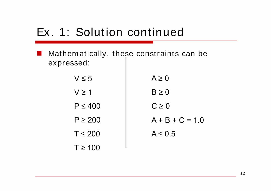
Mathematically, these constraints can be expressed:

V ≤ 5

V ≥ 1

P ≤ 400

P ≥ 200

T ≤ 200

T ≥ 100

A ≥ 0

B ≥ 0

C ≥ 0

A + B + C = 1.0

A ≤ 0.5

13

Ex. 1: Solution continued

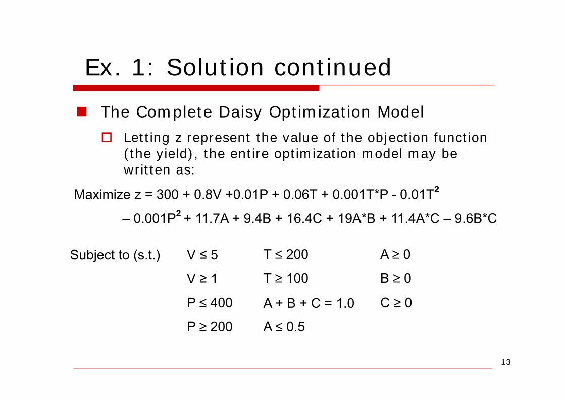
The Complete Daisy Optimization Model

Letting z represent the value of the objection function (the yield), the entire optimization model may be written as:

Maximize z = 300 + 0.8V +0.01P + 0.06T + 0.001T*P - 0.01T2

– 0.001P2 + 11.7A + 9.4B + 16.4C + 19A*B + 11.4A*C – 9.6B*C

V ≤ 5

V ≥ 1

P ≤ 400

P ≥ 200

T ≤ 200

T ≥ 100

A + B + C = 1.0

A ≤ 0.5

A ≥ 0

B ≥ 0

C ≥ 0

Subject to (s.t.)

14

Ex. 1: Solution continued

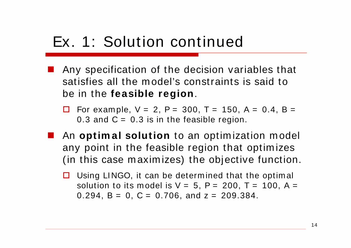
Any specification of the decision variables that satisfies all the model’s constraints is said to be in the feasible region.

For example, V = 2, P = 300, T = 150, A = 0.4, B = 0.3 and C = 0.3 is in the feasible region.

An optimal solution to an optimization model any point in the feasible region that optimizes (in this case maximizes) the objective function.

Using LINGO, it can be determined that the optimal solution to its model is V = 5, P = 200, T = 100, A = 0.294, B = 0, C = 0.706, and z = 209.384.

15

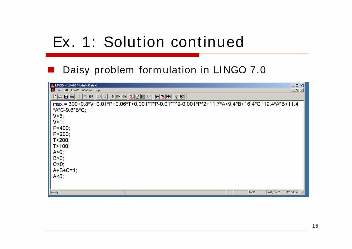
Ex. 1: Solution continued

Daisy problem formulation in LINGO 7.0

16

Ex. 1: Solution continued

Solution extract of Daisy example (shown without slack, surplus, or dual prices) using LINGO 7.0

17

Category of the Models

A static model is one in which the decision variables do not involve sequences of decisions over multiple periods.

A dynamic model is a model in which the decision variables do involve sequences of decisions over multiple periods.

A linear model is one in which the objective function and the constraints are linear.

The Daisy example is a nonlinear model. In general, nonlinear models are much harder to solve.

18

If one or more of the decision variables must be integer, then we say that an optimization model is an integer model.

If all the decision variables are free to assume fractional values, then an optimization model is a noninteger model.

The Daisy example is a noninteger example since volume, pressure, temperature, and percentage composition are all decision variables which may assume fractional values.

Integer models are much harder to solve than noninteger models.

19

A deterministic model is a model in which for any value of the decision variables the value of the objective function and whether or not the constraints are satisfied is known with certainty. If this is not the case, then we have a stochastic model.

If we view the Daisy example as a deterministic model, then we are making the assumption that for given values of V, P, T, A, B, and C the process yield will always be the same.

Since this is unlikely, the objective function can be viewed as the average yield of the process for given decision variable values.

20

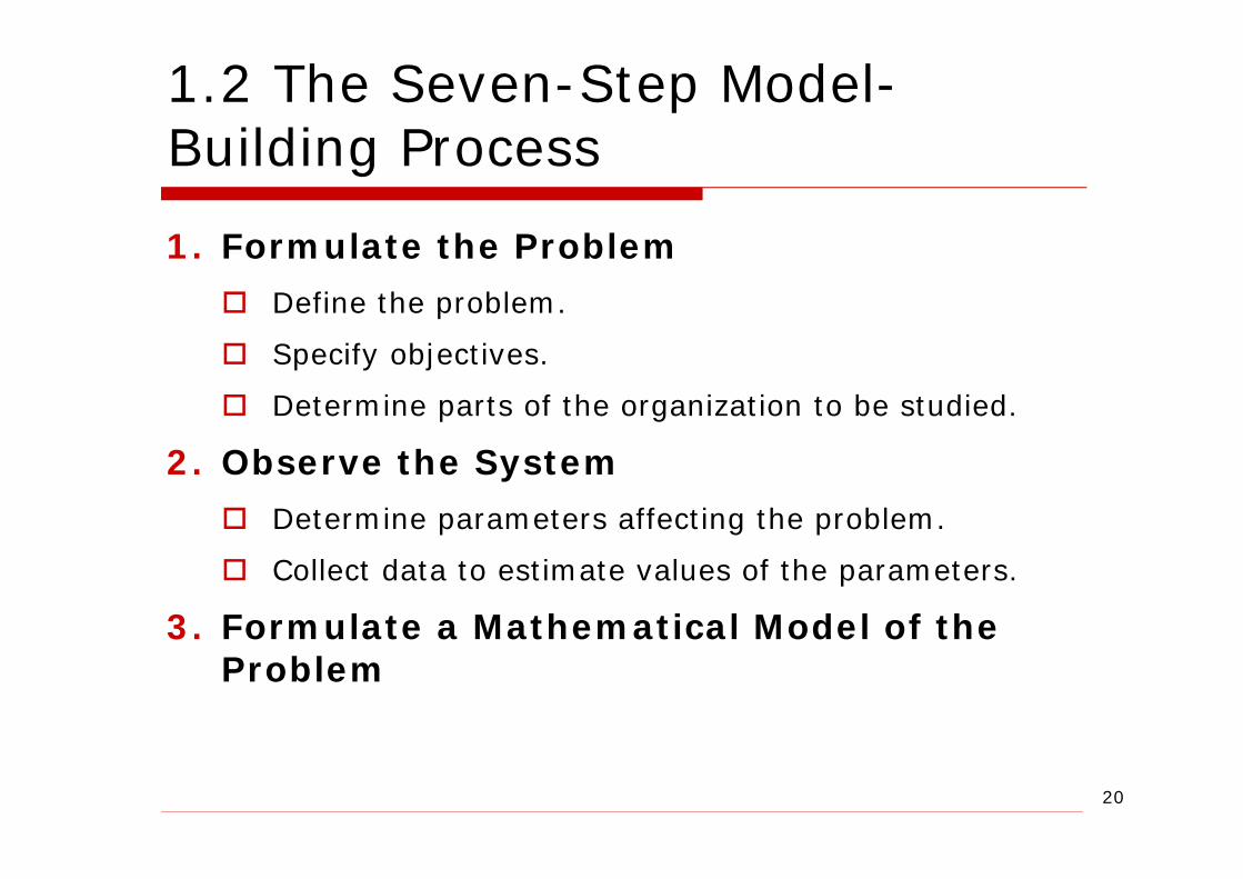
1.2 The Seven-Step Model-Building Process

1. Formulate the Problem

Define the problem.

Specify objectives.

Determine parts of the organization to be studied.

2. Observe the System

Determine parameters affecting the problem.

Collect data to estimate values of the parameters.

3. Formulate a Mathematical Model of the Problem

21

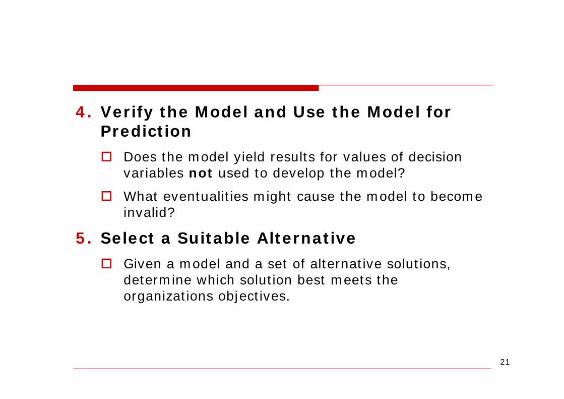
4. Verify the Model and Use the Model for Prediction

Does the model yield results for values of decision variables not used to develop the model?

What eventualities might cause the model to become invalid?

5. Select a Suitable Alternative

Given a model and a set of alternative solutions, determine which solution best meets the organizations objectives.

22

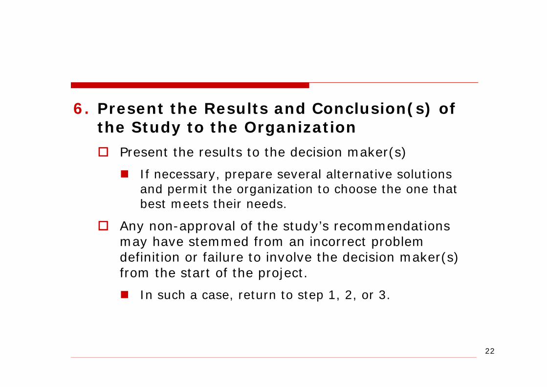
6. Present the Results and Conclusion(s) of the Study to the Organization

Present the results to the decision maker(s)

If necessary, prepare several alternative solutions and permit the organization to choose the one that best meets their needs.

Any non-approval of the study’s recommendations may have stemmed from an incorrect problem definition or failure to involve the decision maker(s) from the start of the project.

In such a case, return to step 1, 2, or 3.

23

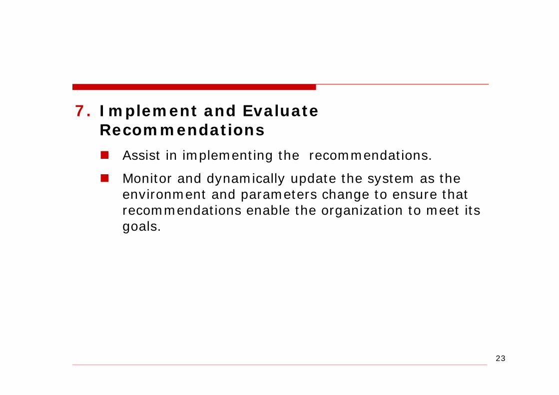
7. Implement and Evaluate Recommendations

Assist in implementing the recommendations.

Monitor and dynamically update the system as the environment and parameters change to ensure that recommendations enable the organization to meet its goals.

24

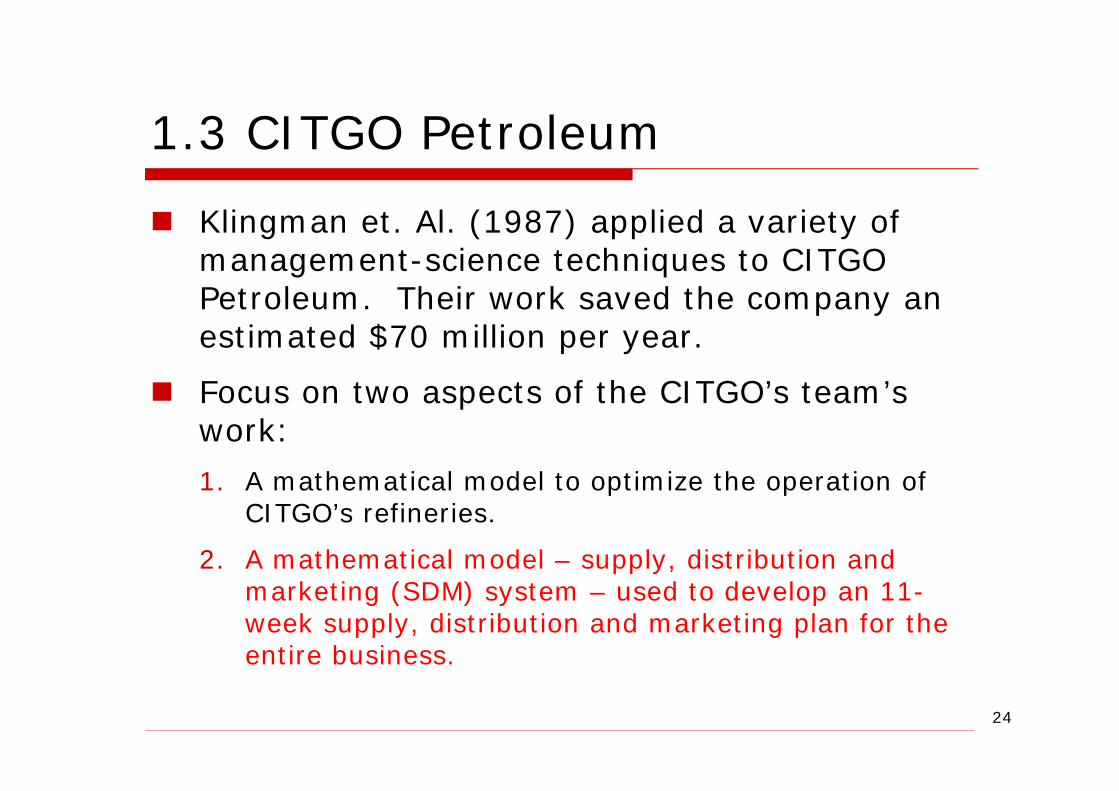
1.3 CITGO Petroleum

Klingman et. Al. (1987) applied a variety of management-science techniques to CITGO Petroleum. Their work saved the company an estimated $70 million per year.

Focus on two aspects of the CITGO’s team’s work:

1. A mathematical model to optimize the operation of CITGO’s refineries.

2. A mathematical model – supply, distribution and marketing (SDM) system – used to develop an 11-week supply, distribution and marketing plan for the entire business.

25

The Supply Distribution Marketing (SDM) System

Step 1 (Formulate the Problem) CITGO wanted a mathematical model that could be used to make supply, distribution, and marketing decisions such as:

Where should the crude oil be purchased?

Where should products be sold?

What price should be charged for products?

How much of each product should be held in inventory?

The goal was to maximize profitability associated with these decisions.

26

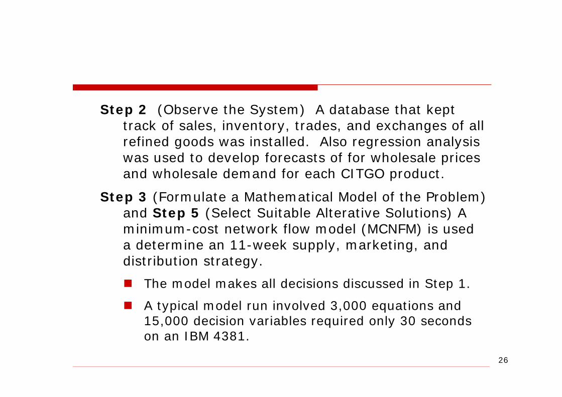
Step 2 (Observe the System) A database that kept track of sales, inventory, trades, and exchanges of all refined goods was installed. Also regression analysis was used to develop forecasts of for wholesale prices and wholesale demand for each CITGO product.

Step 3 (Formulate a Mathematical Model of the Problem) and Step 5 (Select Suitable Alterative Solutions) A minimum-cost network flow model (MCNFM) is used a determine an 11-week supply, marketing, and distribution strategy.

The model makes all decisions discussed in Step 1.

A typical model run involved 3,000 equations and 15,000 decision variables required only 30 seconds on an IBM 4381.

27

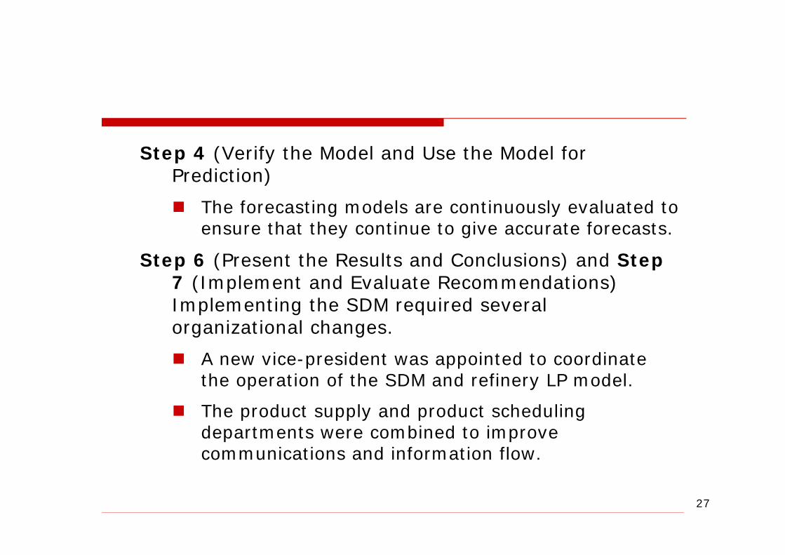
Step 4 (Verify the Model and Use the Model for Prediction)

The forecasting models are continuously evaluated to ensure that they continue to give accurate forecasts.

Step 6 (Present the Results and Conclusions) and Step 7 (Implement and Evaluate Recommendations) Implementing the SDM required several organizational changes.

A new vice-president was appointed to coordinate the operation of the SDM and refinery LP model.

The product supply and product scheduling departments were combined to improve communications and information flow.