CHANNELLING FISHER:

RANDOMIZATION TESTS AND THE STATISTICAL

INSIGNIFICANCE OF SEEMINGLY SIGNIFICANT

EXPERIMENTAL RESULTS*

ALWYN YOUNG

(November 2018, forthcoming, Quarterly Journal of Economics)

I follow R.A. Fisher’s The Design of Experiments (1935), using randomization statistical

inference to test the null hypothesis of no treatment effects in a comprehensive sample of 53

experimental papers drawn from the journals of the American Economic Association. In the

average paper randomization tests of the significance of individual treatment effects find 13 to 22

percent fewer significant results than found using authors’ methods. In joint tests of multiple

treatment effects appearing together in tables, randomization tests yield 33 to 49 percent fewer

statistically significant results than conventional tests. Bootstrap and jackknife methods support

and confirm the randomization results. JEL Codes: C12, C90.

*I am grateful to Larry Katz, Alan Manning, David McKenzie, Ben Olken, Steve Pischke, Jonathan de

Quidt, Eric Verhoogen and anonymous referees for helpful comments, to Ho Veng-Si for numerous conversations,

and to the following scholars (and by extension their co-authors) who, displaying the highest standards of academic

integrity and openness, generously answered questions about their randomization methods and data files: Lori

Beaman, James Berry, Yan Chen, Maurice Doyon, Pascaline Dupas, Hanming Fang, Xavier Giné, Jessica Goldberg,

Dean Karlan, Victor Lavy, Sherry Xin Li, Leigh L. Linden, George Loewenstein, Erzo F.P. Luttmer, Karen Macours,

Jeremy Magruder, Michel André Maréchal, Susanne Neckerman, Nikos Nikiforakis, Rohini Pande, Michael Keith

Price, Jonathan Robinson, Dan-Olof Rooth, Jeremy Tobacman, Christian Vossler, Roberto A. Weber, and Homa

Zarghamee.

2

I: INTRODUCTION

In contemporary economics, randomized experiments are seen as solving the problem of

endogeneity, allowing for the identification and estimation of causal effects. Randomization,

however, has an additional strength: it allows for the construction of tests that are exact, i.e. with

a distribution that is known no matter what the sample size or characteristics of the errors.

Randomized experiments, however, rarely make use of such methods, by and large only

presenting conventional econometric tests using asymptotically accurate clustered/robust

covariance estimates. In this paper I apply randomization tests to 53 randomized experiments,

using them to construct counterparts to conventional tests of the significance of individual

treatment effects, as well as tests of the combined significance of multiple treatment effects

appearing together within regressions or in tables presented by authors. In tests of individual

treatment effects, on average randomization tests reduce the number of significant results relative

to those found by authors by 22 and 13 percent at the .01 level and .05 levels, respectively. The

reduction in rates of statistical significance is greater in higher dimensional tests. In joint tests of

all treatment effects appearing together in tables, for example, on average randomization

inference produces 49 and 33 percent fewer .01 and .05 significant results, respectively, as

comparable conventional tests based upon clustered/robust covariance estimates. Bootstrap and

jackknife methods validate randomization results, producing substantial reductions in rates of

statistical significance relative to authors’ methods.

The discrepancy between the results reported in journals and those found in this paper can

be traced to leverage, a measure of the degree to which individual observations on right-hand side

variables take on extreme values and are influential. A concentration of leverage in a few

observations makes both coefficients and standard errors extremely volatile, as their value

becomes dependent upon the realization of a small number of residuals, generating t-statistic

distributions with much larger tail probabilities than recognized by putative degrees of freedom

and producing sizeable size distortions. I find that the discrepancy between authors’ results and

those based upon randomization, bootstrap or jackknife inference are largely limited to the papers

3

and regressions with concentrated leverage. The results presented by most authors, in the first

table of their main analysis, are generally robust to the use of alternative inference procedures,

but as the data is explored, through the subdivision of the sample or the interaction of treatment

measures with non-treatment covariates, leverage becomes concentrated in a few observations

and large discrepancies appear between authors’ results and those found using alternative

methods. In sum, regression design is systematically worse in some papers, and systematically

deteriorates within papers as authors explore their data, producing less reliable inference using

conventional procedures.

Joint and multiple testing is not a prominent feature of experimental papers (or any other

field in economics), but arguably it should be. In the average paper in my sample, .60 of

regressions contain more than one reported treatment effect.1 When a .01 significant result is

found, on average there are 4.0 reported treatment effects (as well as additional unreported

coefficients on treatment measures), but only 1.6 of these are significant. Despite this, only two

papers report any F tests of the joint significance of all treatment effects within a regression.

Similarly, when a table reports a .01 significant result, on average there are 21.2 reported

treatment effects and only 5.0 of these are significant, but no paper provides combined tests of

significance at the table level. Authors explore their data, independently and at the urging of

seminar participants and referees, interacting treatment with participant covariates within

regressions and varying specifications and samples across columns in tables. Readers need

assistance in evaluating the evidence presented to them in its entirety. Increases in

dimensionality, however, magnify the woes brought on by concentrated leverage, as inaccuracies

in the estimation of high dimensional covariance matrices and extreme tail probabilities translate

into much greater size distortions. One of the central arguments of this paper is that

randomization provides virtually the only reliable approach to accurate inference in high

dimensional joint and multiple testing procedures, as even other computationally intensive

methods, such as the bootstrap, perform poorly in such situations.

1In this paper I use the term regression to refer broadly to an estimation procedure involving dependent and

independent variables that produces coefficients and standard estimates. Most of these are ordinary least squares.

4

Randomization tests have what some consider a major weakness: they provide exact

tests, but only of sharp nulls, i.e. nulls which specify a precise treatment effect for each

participant. Thus, in testing the null of no treatment effects, randomization inference does not

test whether the average treatment effect is zero, but rather whether the treatment effect is zero

for each and every participant. This null is not unreasonable, despite its apparent stringency, as it

merely states that the experimental treatment is irrelevant, a benchmark arguably worth

examining and (hopefully) rejecting. The problem is that randomization tests are not necessarily

robust to deviations away from sharp nulls, as in the presence of unaccounted for heterogeneity in

treatment effects they can have substantial size distortions (Chung & Romano 2013, Bugni,

Canay & Shaikh 2017). This is an important concern, but not one that necessarily invalidates this

paper’s results or its advocacy of randomization methods. First, confirmation from bootstrap and

jackknife results, which test average treatment effects, and the systematic concentration of

differences in high leverage settings, supports the interpretation that the discrepancies between

randomization results and authors’ methods have more to do with size distortions in the latter

than in the former. Second, average treatment effects intrinsically generate treatment dependent

heteroskedasticity, which renders conventional tests inaccurate in finite samples as well. While

robust covariance estimates have asymptotically correct size, asymptotic accuracy in the face of

average treatment effects is equally a feature of randomization inference, provided treatment is

balanced or appropriately studentized statistics are used in the analysis (Janssen 1997, Chung &

Romano 2013, Bugni, Canay & Shaikh 2017). I provide simulations that suggest that, in the face

of heterogeneous treatment effects, t-statistic based randomization tests provide size that is much

more accurate than clustered/robust methods. Moreover, in high dimensional tests randomization

tests appear to provide the only basis for accurate inference, if only of sharp nulls.

This paper takes well-known issues and explores them in a broad practical sample.

Consideration of whether randomization inference yields different results than conventional

inference is not new. Lehmann (1959) showed that in a simple test of binary treatment a

randomization t-test has an asymptotic distribution equal to the conventional t-test, and Imbens

5

and Wooldridge (2009) found little difference between randomization and conventional tests for

binary treatment in a sample of 8 program evaluations. The tendency of White’s (1980) robust

covariance matrix to produce rejection rates higher than nominal size was quickly recognized by

MacKinnon and White (1985), while Chesher and Jewitt (1987) and Chesher (1989) traced the

bias and volatility of these standard error estimates to leverage. This paper links these literatures,

finding that randomization and conventional results are very similar in the low leverage situations

examined in earlier papers, but differ substantially, both in individual results and average

rejection rates, in high leverage conditions, where clustered/robust procedures produce large size

distortions. Several recent papers (Anderson 2008, Heckman et al 2010, Lee & Shaikh 2014,

List, Shaikh & Xu 2016) have explored the robustness of individually significant results to step-

down randomization multiple-testing procedures in a few experiments. This paper, in contrast,

emphasizes the differences between randomization and conventional results in joint and multiple

testing and shows how increases in dimensionality multiply the problems and inaccuracies of

inexact inferential procedures, making randomization inference an all but essential tool in these

methods. It also highlights the practical value of joint tests as an alternative approach with

different power properties than multiple testing procedures.

The paper proceeds as follows: Section II explains the criteria used to select the 53 paper

sample, which uses every paper revealed by a keyword search on the American Economic

Association (AEA) website that provides data and code and allows for randomization inference.

Section III provides background information in the form of a thumbnail review of the role of

leverage in generating volatile coefficients and standard error estimates, the logic and methods of

randomization inference, and the different emphasis of joint and multiple testing procedures.

Section IV uses Monte Carlos to illustrate how unbalanced leverage produces size distortions

using clustered/robust techniques, the comparative robustness of t-statistic based randomization

tests to deviations away from sharp nulls, and the expansion of inaccuracies in high dimensional

testing. Section V provides the analysis of the sample itself, producing the results mentioned

above, while Section VI concludes with some suggestions for improved practice.

6

All of the results of this research are anonymized, as the objective of this paper is to

improve methods, not to target individual results. Thus, no information can be provided, in the

paper, public use files or private discussion, regarding the results for particular papers. For the

sake of transparency, I provide code that shows how each paper was analysed, but the reader

eager to know how a particular paper fared will have to execute this code themselves. A Stata

ado file, available on my website, calculates randomization p-values for most Stata estimation

commands, allowing users to call for randomization tests in their own research.

II. THE SAMPLE

My sample is based upon a search on www.aeaweb.org using the abstract and title

keywords "random" and "experiment" restricted to the American Economic Review (AER),

American Economic Journal (AEJ): Applied Economics and AEJ: Microeconomics which

yielded papers up through the March 2014 issue of the AER. I then dropped papers that:

(a) did not provide public use data files and Stata compatible do-file code; (b) were not randomized experiments;

(c) did not have data on participant characteristics; (d) had no regressions that could be analyzed using randomization inference.

Public use data files are necessary to perform any analysis and I had prior experience with Stata,

which is by far the most popular programme in this literature. My definition of a randomized

experiment excluded natural experiments (e.g. based upon an administrative legal change), but

included laboratory experiments (i.e. experiments taking place in universities or research centres

or recruiting their subjects from such populations). The sessional treatment of laboratory

experiments is not generally explicitly randomized, but when queried laboratory experimenters

indicated that they believed treatment was implicitly randomized through the random arrival of

participants to different sessions. The requirement that the experiment contain data on participant

characteristics was designed to filter out a sample that used mainstream multivariate regression

techniques with estimated coefficients and standard errors.

Not every regression presented in papers based on randomized experiments can be

analyzed using randomization inference. To allow for randomization inference, the regression

7

must contain a common outcome observed under different treatment conditions. This is often not

the case. For example, if participants are randomly given different roles and the potential action

space differs for the two roles (e.g. in the dictator-recipient game), then there is no common

outcome between the two groups that can be examined. In other cases, participants under

different treatment regimes do have common outcomes, but authors evaluate each treatment

regime using a separate regression, without using any explicit inferential procedure to compare

differences. One could, of course, develop appropriate conventional and randomization tests by

stacking the regressions, but this involves an interpretation of the authors’ intent in presenting the

“side-by-side” regressions, which could lead to disputes. I make it a point to adhere to the

precise specification presented in tables.

Within papers, regressions were selected if they allow for and do not already use

randomization inference and:2

(e) appear in a table and involve a coefficient estimate and standard error; (f) pertain to treatment effects and not to an analysis of randomization balance, sample

attrition, or non-experimental cohorts;

while tests were done on the null that:

(g) randomized treatment has no effect, but participant characteristics or other non-randomized treatment conditions might have an influence.

In many tables means are presented, without standard errors or p-values, i.e. without any attempt

at statistical inference. I do not test these. Variations on regressions presented in tables are often

discussed in surrounding text, but interpreting the specification correctly without the aid of the

supplementary information presented in tables is extremely difficult as there are often substantial

do-file inaccuracies. Consequently, I limited myself to specifications presented in tables. Papers

often include tables devoted to an analysis of randomization balance or sample attrition, with the

intent of showing that treatment was uncorrelated with either. I do not include any of these in my

analysis. Similarly, I drop regressions projecting the behaviour of non-treatment cohorts on

treatment measures, which are typically used by authors to, again, reinforce the internal validity

2One paper used randomization inference throughout, and was dropped, while 5 other papers present some

randomization based exact (e.g. Wilcoxon rank sum) tests.

8

of the experiment. In difference in difference equations, I only test the treatment coefficients

associated with differences during the treatment period. I test, universally, the null of no

randomized treatment effect, including treatment interactions with other covariates, while

allowing participant characteristics or non-randomized experimental treatment to influence

behaviour. For example, in the regression

(1) y = α + βTT + βageage + βT*ageT*age + βconvexconvex + βT*convexT*convex + ε

where T is a randomized treatment measure, age is participant age and convex is a non-

randomized payment scheme introduced in later rounds of an experiment, I re-randomize the

allocation of T, repeatedly recalculating T*age and T*convex, and use the distribution of test

statistics to test the null that T, T*age and T*convex have 0 effects on all participants.

I was able to analyze almost all papers and regressions that met the sample selection

guidelines described above. The do files of papers are often inaccurate, producing regressions

that are different from those reported in the published paper, but an analysis of the public use data

files generally allows one to arrive at a specification that, within a small margin of error on

coefficients and standard errors, reproduces the published results. There are only a handful of

regressions, in four papers, that could not be reproduced and included in the sample. To permute

the randomization outcomes of a paper, one needs information on stratification (if any was used)

and the code and methods that produced complicated treatment measures distributed across

different data files. I have called on a large number of authors who have generously answered

questions and provided code to identify strata, create treatment measures and link data files.

Knowing no more than that I was working on a paper on experiments, these authors have

displayed an extraordinary degree of scientific openness and integrity. Only two papers, and an

additional segment from another paper, were dropped from my sample because authors could not

provide the information necessary to re-randomize treatment outcomes.

Table I summarizes the characteristics of my final sample, after reduction based upon the

criteria described above. I examine 53 papers, 14 of which are laboratory experiments and 39 of

which are field experiments. 27 of the papers appeared in the AER, 21 in the AEJ: Applied

9

Economics, and 5 in the AEJ: Microeconomics. The number of tables reporting estimates and

standard errors for treatment effects that I am able to analyze using randomization inference

varies substantially across papers, with 17 papers having only 1 or 2 such tables and 19

presenting 5 to 8. The number of coefficients reported in these tables varies even more, with one

paper reporting 260 treatment coefficients and another only 2. I deal with the heterogeneity in

the number of treatment results by adopting the convention of always reporting the average

across papers of the within paper average measure, so that each paper, regardless of the number

of coefficients, regressions or tables, carries an equal weight in summary statistics. Although

most papers report all of the treatment effects in their estimating equations, some papers do not,

and the number of such unreported auxiliary coefficients ranges from 1 to 48 in 7 papers to 76 to

744 in 5 papers. To avoid the distracting charge that I tested irrelevant treatment characteristics, I

restrict the analysis below to reported coefficients. Results which include unreported treatment

effects, in the on-line appendix, exhibit very much the same patterns.

My sample contains 1780 regressions, broadly defined as a self-contained estimation

procedure with dependent and independent variables that produces coefficient estimates and

standard errors. In the average paper, 67 percent of these are ordinary least squares regressions

(including weighted), 22 percent involve maximum likelihood estimation (mostly discrete choice

models), and the remaining 11 percent include handfuls of quantile regressions, two-step

Heckman models, and other methods. In the typical paper, one-quarter of regressions make use

of Stata's default (i.e. homoskedastic) covariance matrix calculation, 70 percent avail themselves

of clustered/robust estimates of covariance, 4 percent use the bootstrap, and the remaining 2

percent use hc2/hc3 type corrections of clustered/robust covariance estimates. In 171 regressions

in 12 papers (8 lab, 4 field) treatment is applied to groups, but the authors do not cluster or

systematically cluster at a lower level of aggregation. This is not best practice, as correlations

between the residuals for individuals playing games together in a lab or living in the same

geographical region are quite likely. By clustering at below treatment level, these authors treat

the grouping of observations in laboratory sessions or geographical areas as nominal. In

10

)1(

ˆ

~

~ˆˆ

2~

ii

i

i

i

i

ihx

x

−−=∑

εββ

implementing randomization, bootstrap and jackknife inference in this paper, I defer to this

judgement, randomizing and sampling at the level at which they clustered (or didn’t), treating the

actual treatment grouping as irrelevant. Results with randomization and sampling at the

treatment level, reported in the on-line appendix, find far fewer significant treatment effects.3

III: ISSUES AND METHODS

III.A. Problems of Conventional Inference in Practical Application

One of the central characteristics of my sample is its remarkable sensitivity to outliers.

Panel A of Figure I plots the maximum and minimum coefficient p-values, using author's

methods, found when one deletes one cluster or observation at a time from each regression in my

sample against the p-value found with the full sample.4 With the removal of just one observation,

.35 of .01 significant reported results in the average paper can be rendered insignificant at that

level. Conversely, .16 of .01 insignificant reported results can be found to be significant at that

level. Panel B of the figure graphs the difference between these maximum and minimum p-

values against the number of clusters/observations in the regression. In the average paper the

mean difference between the maximum and minimum delete-one p-values is .23. To be sure, the

problem is more acute in smaller samples, but surprising sensitivity can be found in samples with

1000 clusters or observations and even in those with more than 50000 observations.

A few simple formulas identify the sources of delete-one sensitivity. In OLS regressions,

which make up much of my sample, the coefficient estimate with observation i removed ( i~β ) is

related to the coefficient estimate from the full sample ( β ) through the formula:

(2)

where ix~ denotes the ith

residual from the projection of independent variable x on the other

3In another 3 papers, the authors generally cluster at treatment level, but fail to cluster a few regressions. I

randomize these at the treatment level so as to calculate the joint distribution of coefficients across equations. In 3

papers where the authors cluster across treatment groupings, I rerandomize at the treatment level.

4Where authors cluster, I delete clusters; otherwise I delete individual observations.

11

.~

~~ where,ˆ

~~

12

2

2

2 ∑∑

∑=

−i

i

i

iiiii

i x

xh

kn

nh

xε

regressors in the n x k matrix of regressors X, iε the ith

residual of the full regression, and hii,

commonly known as leverage, is the ith

diagonal element of the hat matrix XX)XX(H 1 ′′= − .5

The robust variance estimate can be expressed as

(3)

iih~

might be termed coefficient leverage, because it is the ith diagonal element of the hat matrix

x)xx(xH1 ′= − ~~'~~~

for the partitioned regression. As seen in (2) and (3), when coefficient leverage

is concentrated in a few observations, coefficient and standard error estimates, depending upon

the realization of residuals, are potentially sensitive to the deletion of those observations.

Sensitivity to a change in the sample is an indication that results are dependent upon the

realizations of a small set of disturbances. In non-iid settings, this translates into inaccurate

inference for a given sample, the object of interest in this paper. The summation in (3) is a

weighted average as iih~

varies between 0 and 1 and sums to 1 across all observations. With

concentrated leverage, robust standard error estimates depend heavily on a small set of stochastic

disturbances and become intrinsically more volatile, producing t-statistic distributions that are

more dispersed than recognized by nominal degrees of freedom. When the effects of right-hand

side variables are heterogeneous, the residuals have a heteroskedastic variance that is increasing

in the magnitude of the regressor. This makes the robust standard error even more volatile, as it

now places a disproportionate weight on disproportionately volatile residuals. Concentrated

leverage also shrinks estimated residuals, as coefficient estimates respond to the realization of the

disturbance, so a heavy weight is placed on residuals which are biased towards zero, biasing the

standard error estimate in the same direction.6 Thus, the estimates of the volatility of coefficients

5So-called because .ˆ Hyy = The formula for the deletion of vector i of clustered observations is

).~~/(ˆ)(~ˆˆ 1 xxεHIx iiiiii~′−′−= −ββ When the coefficient on a variable is determined by an individual observation or

cluster, hii equals 1 or (in the cluster case) Ii - Hii is singular. In this case, the delete-i formula for the remaining

coefficients calculates Hii using the residuals of the remaining regressors projected on the variable in question.

6As an extreme example, when coefficient leverage for observation i is 1, i

ˆ yyi = , the estimated residual for i

is always 0 and the robust standard error estimate for the coefficient is 0 as well.

12

and of the volatility of the standard error are both biased downwards, producing t-statistic

distributions with underappreciated tail probabilities.

Table II reports the total coefficient leverage accounted for by the clusters or observations

with the largest leverage in my sample. I calculate the observation level shares iih~

, sum across

observations within clusters if the regression is clustered, and then report the average across

papers of the within paper mean share of the cluster/observation with the largest coefficient

leverage ("max"), as well as the total leverage share accounted for by largest 1st, 5

th and 10

th

percentiles of the distribution. I include measures for non-OLS regressions in these averages as

well, as all of these contain a linear xiʹβ term and leverage plays a similar role in their standard

error estimates.7 As shown in the table, in the mean paper the largest cluster/observation has a

leverage of .058, while the top 1st and 10

th percentiles account for .091 and .338 of total leverage,

respectively. These shares vary substantially by paper. Dividing the sample into thirds based

upon the average within paper share of the maximal cluster/observation, one sees that in the low

leverage third the average share of this cluster/observation is .008, while in the high leverage

third it is .134 (with a mean as high as .335 in one paper).

Table II also compares the concentration of leverage in the very first table where authors

present their main results against later tables, in papers which have more than one table reporting

treatment effects.8 Leverage is more concentrated in later tables, as authors examine subsets of

the sample or interact treatment with non-treatment covariates. Specifically comparing

coefficients appearing in regressions where treatment is interacted with covariates against those

where it is not, in papers which contain both types of regressions, we see that regressions with

covariates have more concentrated leverage. The presence of non-treatment covariates in the

regression per say, however, does not have a very strong effect on coefficient leverage, as the

7Thus, the oft used robust covariance for matrix maximum likelihood models can be re-expressed as ARAʹ,

where, with D1 and D2 denoting diagonal matrices of the observational level 1st and 2

nd derivatives of the ln-

likelihood with respect to xiʹβ, R = (XʹX)-1

(XʹD1D1X)(XʹX)-1

& A = (-XʹD2X)-1

XʹX. With D1 serving as the residual,

leverage plays the same role in determining the elements of R as it does in the OLS covariance estimate.

8Main results are identified as the first section with this title (a frequent feature) or a title describing an

outcome of the experiment (e.g. “Does treatment-name affect interesting-outcome?”).

13

table shows by recalculating treatment coefficient leverage shares with non-treatment covariates

excluded from the regression (but treatment interactions with covariates retained). This is to be

expected if covariates are largely orthogonal to treatment.

A few examples illustrate how regression design can lead to concentrated leverage.

Binary treatment applied 50/50 to the entire sample, with otherwise only a constant term in the

regression, produces uniform leverage. Apply three binary treatments and control each to ¼ of

the population, and in a joint regression with a constant term each treatment arm concentrates the

entirety of leverage in ½ of the observations. The clustered/robust covariance estimate is now

based on only half of the residuals and consequently has a volatility (degrees of freedom)

consistent with half the sample size. Run, as is often done, the regression using only one of the

three treatment measures as a right hand side variable, so that binary treatment in the regression is

applied in 25/75 proportions, and ¼ of observations account for ¾ of leverage. Apply 50/50

binary treatment, and create a second treatment measure by interacting it with a participant

characteristic that rises uniformly in even discrete increments within treatment and control, and ⅕

of observations account for about ⅗ of coefficient leverage for the binary treatment measure

(even without the non-treatment characteristic in the regression). Seemingly innocuous

adjustments in regression design away from the binary 50/50 baseline generate substantially

unbalanced leverage, producing clustered/robust covariance estimates and t-statistics which are

much more dispersed than recognized.

III.B. Randomization Statistical Inference

Randomization inference provides exact tests of sharp (i.e. precise) hypotheses

no matter what the sample size, regression design or characteristics of the disturbance term. The

typical experimental regression can be described as yE = TEβt + Xβx + ɛ, where yE is the n x 1

vector of experimental outcomes, TE an n x t matrix of treatment variables (including possibly

interactions with non-treatment covariates), and X an n x k matrix of non-randomized covariates.

Conventional econometrics describes the statistical distribution of the estimated βs as coming

from the stochastic draw of the disturbance term ɛ, and possibly the regressors, from a population

14

∑∑==

=+>=M

1

ES

M

1

ES )T(IM

1*)T(I

M

1 value-pionrandomizat

SS

U

distribution. In contrast, in randomization inference the motivating thought experiment is that,

given the sample of experimental participants, the only stochastic element determining the

realization of outcomes is the randomized allocation of treatment. For each participant, the

observed outcome yi is conceived as a determinate function of the treatment ti allocated to that

participant, yi(ti). Consequently, the known universe of potential treatment allocations

determines the statistical distribution of the estimated βs and can be used to test sharp hypotheses

which precisely specify the treatment effect for each participant, because sharp hypotheses of this

sort allow the calculation of what outcomes would have been for any potential random allocation

of treatment. Consider for example the null hypothesis that the treatment effects in the equation

above equal β0 for all participants. Under this null, the outcome vector that would have been

observed had the treatment allocation been TS rather TE is given by yS = yE - TEβ0 + TSβ0 and this

value, along with TS and the invariant characteristics X can be used to calculate estimation

outcomes under treatment allocation TS.9

An exact test of a sharp null is constructed by calculating possible realizations of a test

statistic and rejecting if the observed realization in the experiment itself is extreme enough. In

the typical experiment there is a finite set Ω of equally probable potential treatment allocations

TS. Let f(TE) denote a test statistic calculated using the treatment applied in the experiment and

f(TS) the known (under the sharp null) value the statistic would have taken if the treatment

allocation had been TS. If the total number of potential treatment allocations in Ω is M, the p-

value of the experiment’s test statistic is given by:

(4)

where IS(>TE) and IS(=TE) are indicator functions for f(TS) > f(TE) and f(TS) = f(TE),

respectively, and U is a random variable drawn from the uniform distribution. In words, the p-

value of the randomization test equals the fraction of potential outcomes that have a more

9Imbens & Rubin (2015) provide a thorough presentation of inference using randomized experiments,

contrasting and exploring the Fisherian potential outcomes and Neymanian population sampling approaches.

15

=++

+>+

= ∑∑==

N

1

ES

N

1

ES )T(I11N

1*)T(I

1N

1 value-pionrandomizat sampling

SS

U

extreme test statistic added to the fraction that have an equal test statistic times a uniformly

distributed random number. In the on-line appendix I prove that this p-value is uniformly

distributed, i.e. the test is exact with a rejection probability equal to the nominal level of the test.

Calculating (4), evaluating f(TS) for all possible treatment realizations in Ω, is generally

impractical. However, under the null random sampling with replacement from Ω allows the

calculation of an equally exact p-value provided the original treatment result is automatically

counted as a tie with itself. Specifically, with N additional draws (beyond the original treatment)

from Ω, the p-value of the experimental result is given by:

(5)

In the on-line I appendix I show that this p-value is uniformly distributed regardless of the

number of draws N used in its evaluation.10 This establishes that size always equals nominal

value, even though the full distribution of randomization outcomes is not calculated. However,

power, provided it is a concave function of the nominal size of the test, is increasing in N (Jockel

1986). Intuitively, as the number of draws increases the procedure is better able to identify what

constitutes an outlier outcome in the distribution of the test statistic f(). In my analysis, I use

10000 draws to evaluate (5). When compared with results calculated with fewer draws, I find no

appreciable change in rejection rates beyond 2000 draws.

One drawback of randomization inference, easily missed in the short presentation above,

is that in equations with multiple treatment measures the p-value of the null for one coefficient

generally depends upon the null assumed for other treatment measures, as these nulls influence

the outcome yS that would have been observed for treatment allocation TS. It is possible in some

multi-treatment cases to calculate p-values for individual treatment measures that do not depend

upon the null for other treatments by considering a subset of the universe of potential

10

The proof is a simple extension of Jockel’s (1986) result for nominal size equal to a multiple of 1/(N+1). It

generalizes to treatment allocations that are not equally probable by simply duplicating each treatment outcome in Ω

according to its relative frequency, so that each element in Ω becomes equally likely.

16

)ˆˆ(ˆ)(ˆ)(ˆ)(ˆSSS Et

1

EtEtt

1

tt (Tβ))(Tβ)V(TβTβ)TβV(Tβ−− ′≥′

randomization allocations that holds other treatments constant.11

Such calculations, however,

must be undertaken with care, as there are many environments where it is not possible to

conceive of holding one treatment measure constant while varying another.12 In results reported

in this paper, I always test the null that all treatment effects are zero and all reported p-values for

joint or individual test statistics are under that joint null. In the on-line appendix I calculate,

where possible, alternative p-values for individual treatment effects in multi-treatment equations

that do not depend upon the null for other treatment measures. On average, the results are less

favourable to my sample (i.e. reject less often and produce bigger p-value changes).

I make use of two randomization based test statistics, which find counterparts in

commonly used bootstrap tests. The first is based upon a comparison of the Wald statistics of the

conventional tests of the significance of treatment effects, as given by )(ˆ)(ˆ)(ˆSSS Tβ)TβV(Tβ t

1

tt

−′ ,

where tβ and )βV( t

ˆ are the regression’s treatment coefficients and the estimated covariance

matrix of those coefficients. This method in effect calculates the probability

(6)

I use the notation (TS) to emphasize that both the coefficients and covariance matrix are

calculated for each realization of the random draw TS from Ω. This test might be termed the

randomization-t, as in the univariate case it reduces to a comparison of squared t-statistics. It

corresponds to bootstrap tests based upon the percentiles of Wald statistics.

An alternative test of no treatment effects is to compare the relative values of

)(ˆ)(ˆ)(ˆSS Tβ)ΩβV(Tβ t

1

tt

−′ , where )ΩβV( t )(ˆ is the covariance of tβ across the universe of potential

11

Consider the case with control and two mutually exclusive treatment regimes denoted by the dummy

variables T1 and T2. Holding the allocation of T2 constant (for example), one can re-randomize T1 across those who

received T1 or control, modifying y for the hypothesized effects of T1 only, and calculate a p-value for the effect of

T1 that does not depend upon the null for T2.

12Consider, for example, the case of treatment interactions with covariates (which arises frequently in my

sample), as in the equation y = α + βTT + βageage + βT*ageT*age + ε. It is not possible to re-randomize T holding

T*age constant, or to change T*age while holding T constant, so there is no way to calculate a p-value for either

effect without taking a stand on the null for the other.

17

)(ˆ)(ˆ)(ˆ)(ˆ)(ˆ)(ˆ( SS Et

1

tEtt

1

tt Tβ)ΩβV(TβTβ)ΩβV(Tβ−− ′≥′

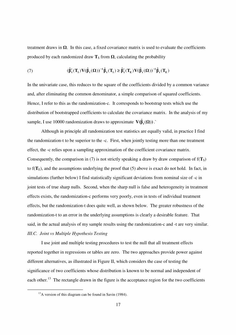
treatment draws in Ω. In this case, a fixed covariance matrix is used to evaluate the coefficients

produced by each randomized draw TS from Ω, calculating the probability

(7)

In the univariate case, this reduces to the square of the coefficients divided by a common variance

and, after eliminating the common denominator, a simple comparison of squared coefficients.

Hence, I refer to this as the randomization-c. It corresponds to bootstrap tests which use the

distribution of bootstrapped coefficients to calculate the covariance matrix. In the analysis of my

sample, I use 10000 randomization draws to approximate )ΩβV( t )(ˆ .`

Although in principle all randomization test statistics are equally valid, in practice I find

the randomization-t to be superior to the -c. First, when jointly testing more than one treatment

effect, the -c relies upon a sampling approximation of the coefficient covariance matrix.

Consequently, the comparison in (7) is not strictly speaking a draw by draw comparison of f(TS)

to f(TE), and the assumptions underlying the proof that (5) above is exact do not hold. In fact, in

simulations (further below) I find statistically significant deviations from nominal size of -c in

joint tests of true sharp nulls. Second, when the sharp null is false and heterogeneity in treatment

effects exists, the randomization-c performs very poorly, even in tests of individual treatment

effects, but the randomization-t does quite well, as shown below. The greater robustness of the

randomization-t to an error in the underlying assumptions is clearly a desirable feature. That

said, in the actual analysis of my sample results using the randomization-c and -t are very similar.

III.C. Joint vs Multiple Hypothesis Testing

I use joint and multiple testing procedures to test the null that all treatment effects

reported together in regressions or tables are zero. The two approaches provide power against

different alternatives, as illustrated in Figure II, which considers the case of testing the

significance of two coefficients whose distribution is known to be normal and independent of

each other.13

The rectangle drawn in the figure is the acceptance region for the two coefficients

13

A version of this diagram can be found in Savin (1984).

18

tested individually with a multiple testing adjustment to critical values, while the oval drawn in

the figure is the Wald acceptance region for the joint significance of the two coefficients. In the

multiple testing framework, to keep the probability of one or more Type I errors across the two

tests at level α, one could select a size η for each test such that 1-(1-η)2 = α. The probability of

no rejections, under the null, given by the integral of the probability density inside the rectangle,

then equals 1-α. The integral of the probability density inside the Wald ellipse is also 1-α. The

Wald ellipse, however, is the translation-invariant procedure that minimizes the area such that the

probability of falling in the acceptance region is 1-α.14

It achieves this, relative to the multiple

testing rectangle, by dropping corners, where the probability of two extreme outcomes is low, and

increasing the acceptance region along the axes. Consequently, the joint test has greater power to

reject in favour of alternatives within quadrants, while multiple testing has greater power to reject

when alternatives lie on axes. In the analysis of the experimental sample further below I find that

joint testing produces rejection rates that are generally slightly greater than those found using

multiple testing procedures, i.e. while articles emphasize the extreme effects of individual

statistically significant treatment measures, evidence in favour of the relevance of treatment is at

least as often found in the modest effects of multiple aspects of treatment.

Multiple testing is an evolving literature. The classical Bonferroni method evaluates each

test at the α/N level, which, based on Boole’s inequality, ensures that the probability of a Type I

error in N tests is less than or equal to α no matter what the correlation between the test statistics.

For values of α such as .01 or .05, the gap between α/N and the p-value cutoff η = 1-(1-α)1/N

that

would be appropriate if the test statistics were known to be independent, as in the example above,

is miniscule. Nevertheless, as Bonferroni’s method does not make use of information on the

covariance of p-values, it can be quite conservative. For example, if the p-values of individual

tests are perfectly correlated under the null, then α is the αth percentile of their minimum and

hence provides an α probability of a Type I error when applied to all tests. In recognition of this,

14

A procedure is translation invariant if, after adding a constant to both the point estimate and the null, one

remains in the confidence region. Stein (1962) provides examples of procedures that do not satisfy this requirement

but produce smaller confidence regions.

19

Westfall & Young (1993) suggested using bootstrap or randomization inference to calculate the

joint-distribution of p-values and then using the αth

percentile of the minimum as the cutoff value.

In the analysis of the sample below I find that Westfall & Young’s procedure yields substantially

higher rejection rates than Bonferroni’s method in table level tests of treatment effects, as

coefficients appearing in different columns of tables are often highly (if not perfectly) correlated.

While joint testing produces a single 0/1 decision, multiple testing allows for further tests,

as following an initial rejection one can step-down through the remaining tests using less

demanding cutoffs (e.g. Holm 1979, Westfall & Young 1993). Step-down procedures of this sort

require either “subset pivotality” (Westfall & Young 1993), i.e. that the multivariate distribution

of p-values for subsets of hypotheses does not depend upon the truth of other hypotheses, or,

more generally, that critical values are weakly monotonic in subsets of hypotheses (Romano &

Wolf 2005). Both conditions trivially hold when authors kindly project a different dependent

variable on a single treatment measure in each column of a table. This rarely occurs. Within

equations, treatment measures are interacted with covariates, making the calculation of a

randomization distribution without an operational null on each treatment measure impossible, as

noted earlier. Across columns of tables the same dependent variable is usually projected on

slightly different specifications or sub-samples, making the existence of non-zero effects in one

specification and a sharp null in another logically impossible.15 However, the null that every

aspect of treatment has zero effects everywhere on everyone can always be tested.

I use joint and multiple testing procedures in this paper to highlight the relevance of

randomization inference in these, as the size distortions of inexact methods are much larger in

higher dimensional joint tests and in evaluating extreme tail probabilities. In multiple testing I

restrict attention to the existence of any rejection, as this initial test can be applied to any group of

results in my sample. Alternative multiple testing procedures all start with the same initial

15

As examples: (i) having rejected the null of zero effects for women, it is not possible to consider a sharp null

of zero in an equation that combines men and women; (ii) having rejected the null of zero effects in the projection of

an outcome on treatment and covariates, it is not possible to then consider a sharp null of zero in the projection of the

outcome on treatment alone.

20

Bonferroni or Westfall-Young cutoff, and hence their initial decisions are subsumed in those

results.16

The existence of any rejection in multiple testing also produces a result equivalent to

the joint test, i.e. a statement that the combined null is false, allowing a comparison of the two

methods and of the evidentiary value of traditionally emphasized treatment effects on axes

against that provided by the combinations of treatment effects found within quadrants.

IV: MONTE CARLOS

In this section I use simulations with balanced and unbalanced regression design and fixed

and heterogeneous treatment effects to compare rejection rates of true nulls using clustered/robust

covariance estimates to results obtained using randomization inference, as well as those found

using the bootstrap and jackknife. For randomization inference and the bootstrap I use the

randomized and bootstrapped distribution of coefficients and robust t-statistics to evaluate the p-

value, i.e. the -c and -t methods described earlier in (6) and (7). The bootstrap-t is generally

considered superior to the -c as its rejection probabilities converge more rapidly asymptotically to

nominal size (Hall 1992). For OLS regressions, the jackknife substitutes ε~i, the residual for

observation i when the delete-i coefficient estimates are used to calculate predicted values for that

observation, for the [n/(n-k)]-½

adjusted estimated residual used in the clustered/robust formula

(3) earlier, which has the disadvantage of being biased toward zero in high leverage observations.

It is equivalent to the hc3 finite sample correction of clustered/robust covariance estimates, which

appears to provide better inference in finite samples (MacKinnon and White 1995).

Table III reports size at the .05 level of the different methods in tests of individual

coefficients. Panel A uses the data generating process yi = α + tiβi + ɛi, with εi distributed iid

standard normal and ti a 0/1 treatment measure that is administered in a balanced (50/50) or

unbalanced (10/90) fashion. For βi, I consider both fixed treatment effects, with βi = β for all

observations, and heterogeneous treatment effects, with βi distributed iid standard normal or iid

chi2. Panel B uses the data generating process yi = α + ti*βi + ti*xi*γi + xi + ɛi, where εi is again

16

Thus, for example, control of the false discovery rate at rate α using Benjamini & Hochberg’s (1995) step-

down procedure imposes a rejection criterion of α/N for the first step.

21

distributed iid normal and ti is a 0/1 treatment measure administered in a balanced (50/50)

fashion. Treatment interacts with a participant characteristic xi, which is distributed iid

exponential with mean 1. Once again, the parameters βi and γi are either fixed or distributed iid

normal or chi2. Sample sizes range from 20 to 2000. In each case, I use OLS to estimate average

treatment effects in a specification that follows the data generating process. With 10000

simulations there is a .99 probability of estimated size lying between .044 and .056 if the

rejection probability is actually .05.

Two patterns emerge in Table III. First, with evenly distributed leverage, all methods,

with the exception perhaps of the bootstrap-c, do reasonably well. This is apparent in the left-

hand side of (A), where leverage is evenly distributed in all samples, but also in the rapid

convergence of size to nominal value with unbalanced regression design in the right-hand side of

(A), where the maximal leverage of a single observation falls from .45 to .045 to .0045 with the

increase in the sample size. Things proceed much less smoothly, however, in Panel B where the

exponentially distributed covariate ensures that the maximal observation leverage share remains

above .029 (and as high as .11) more than ¼ of the time even in samples with 2000 observations.

Asymptotic theorems rely upon an averaging that is precluded when estimation places a heavy

weight on a small number of observations, so regression design rather than the crude number of

observations is probably a better guide to the quality of inference based upon these theorems.

Second, Table III shows that the randomization-t is much more robust than the -c to

deviations from the sharp null. When heterogeneous treatment effects that are not accounted for

in the randomization test are introduced, rejection rates using the randomization-c rise well above

nominal value, but the randomization-t continues to do well, with rejection probabilities that are

closer to nominal size than any method other than the bootstrap-t. The intuition for this result is

fairly simple. Heterogeneous treatment effects introduce heteroskedasticity that is correlated

with extreme values of the regressors, making coefficient estimates more volatile. When

treatment is re-randomized with a sharp null adjustment to the dependent variable equal to the

mean treatment effect of the data generating process, the average treatment effect is retained, but

22

the correlation between the residual and the treatment regressor is broken, so the coefficient

estimate becomes much less volatile. When the deviation of the original coefficient estimate

from the null is compared to this randomized distribution of coefficients, it appears to be an

outlier, generating a randomization-c rejection probability well in excess of nominal size, as

shown in the table. In contrast, the randomization-t adjusts the initial coefficient deviation from

the null using its large robust standard error estimate and all the later, less volatile, coefficient

deviations from the null using the much smaller robust standard error estimates that arise when

heteroskedasticity is no longer correlated with the regressors. By implicitly taking into account

how re-randomization reduces the correlation between heteroskedastic residuals and the

treatment regressor, the randomization-t adjusts for how re-randomization reduces the dispersion

of coefficient estimates around the null.

Table IV evaluates rejection rates of the different methods in joint and multiple tests of

the significance of treatment effects in 10 independent equations of the form used in Panel A of

Table III. The top panel reports the frequency with which at least one true null is rejected using

the Bonferroni multiple testing critical value of .05/10 = .005. The bottom panel reports the

frequency with which the joint null that all 10 coefficients equal the data generating value are

rejected, using White’s (1982) extension of the robust covariance method to estimate the

covariance of the treatment coefficients across equations for the conventional Wald statistic and

the randomization and bootstrap estimates of its distribution. The most notable difference in the

pattern of results, relative to Table III, is the magnitude of the size distortions. In small samples

the robust and jackknife approaches have rejection probabilities approaching 1.0, particularly in

joint tests, while bootstrap rejection probabilities range from 0 to well above .05, but are rarely

near .05. Even with perfectly balanced leverage, in small samples joint and multiple tests often

have rejection probabilities that are well outside the .99 probability interval for an exact test.17

17

As noted earlier, in joint tests the randomization-c is no longer exact even in tests of sharp nulls, as the

covariance matrix in the calculation of the distribution of test statistics (7) is only an approximation to the covariance

matrix across all possible randomization draws. This is clearly seen in the rejection probabilities of .060 and .058 in

samples of 20 in panel (B1).

23

wVw

βwβVβ

w

1

ˆ

)ˆ(Maxˆˆˆ

2

′′

=′ −

Size distortions increase with dimensionality in joint and multiple tests for different

reasons. In the case of multiple tests, the problem is that a change in the thickness of the tails of a

distribution generally results in a proportionally greater deviation at more extreme tail values.

Thus, a test that has twice (or one-half) the nominal rejection probability at the .05 level will

typically have more than twice (less than one-half) the nominal rejection probability at the .005

level. Consequently, as N increases and the α/N Bonferroni cutoff falls, the probability of a

rejection across any of the N coefficients will deviate further from its nominal value, so small

size distortions in the test of one coefficient become large size distortions in the test of N. In the

case of joint tests, intuition can be found by noting that the Wald statistic is actually the

maximum squared t-statistic that can be found by searching over all possible linear combinations

w of the estimated coefficients (Anderson 2003), that is:

(8)

When the covariance estimate equals the true covariance matrix V times a scalar error, i.e.

22 /ˆˆ σσVV = , as is the case with homoskedastic errors and covariance estimates, this search is

actually very limited and produces a variable with a chi2 or F distribution.

18 However, when V is

no simple scalar multiple of the true covariance V, the search possibilities expand, allowing for

much larger tail outcomes. This systematically produces rejection probabilities much greater

than size in clustered/robust joint tests.19

At the same time, if the bootstrapped or randomized

distribution of V is even slightly misrepresentative of its true distribution, the two methods can

18Employing the transformations wVw

½~ = and βVβ ˆ~ ½−= , plus the normalization 1~~ =′ww :

22½½

2

~

2

/ˆ

~~

~ˆ~)

~~(Max

ˆ

)ˆ(Max

σσββ

wVVVw

βw

wVw

βw

ww

′=

′′

=′′

−−

The last equality follows because the denominator reduces to 22 /ˆ σσ no matter what the w~ such that 1~~ =′ww ,

while the maximum of the numerator across w~ equals ββ~~′ , which is typically an independent chi

2 variable with k

degrees of freedom (dof). Thus, the maximum is either distributed chi2 with k dof (when asymptotically 22ˆ σσ = )

or else equals k times an Fk,n-k (when the denominator is (n-k)-1

times a chi2 variable with n-k dof). However, when

22 /ˆˆ σσVV ≠ the search possibilities in the denominator clearly expand.

19Young (2018) provides further evidence of this for the case of F-tests of coefficients in a single regression.

24

greatly over or understate the search possibilities in the original procedure, producing large size

distortions of their own. Thinking of a joint test as a maximization problem provides, I believe,

some intuition for why errors in approximating the distribution increase with the dimensionality

of the test.

Figure III graphs randomization-t p-values against those found using conventional

techniques. In each panel I take the first 1000 results from each of the three data generating

processes for parameters (fixed, normal & chi2), comparing results with small (N = 20) and large

(N = 2000) samples. Panel A graphs p-values from the balanced regression design of the upper-

left hand panel of Table III, where robust p-values are nearly exact in both small and large

samples, showing that randomization and conventional p-values are almost identical in both

cases. Panel B graphs the p-values of the lower-right hand panel of Table III, where robust

methods have positive size distortions in small samples. In small samples, randomization p-

values are concentrated above conventional results, with particularly large gaps for statistically

significant results, but in large samples the two types of results are, once again, almost identical.

Panel C graphs the joint tests of the lower-left hand panel of Table IV, where robust methods

produce large size distortions in small samples but have accurate size in large samples. In small

samples the pattern of randomization p-values lying above robust results, particularly for small

conventional p-values, is accentuated, but once again differences all but disappear in large

samples.20

Panels A - C of Figure III might lead to the conclusion that randomization and

conventional p-values agree in large samples or when both p-values are nearly exact. Panel D

shows this is not the case by examining conventional inference with the default homoskedastic

covariance estimate for the highly leveraged coefficients tested in the lower left-hand panel of

Table III. With samples of 20 observations, despite the fact that errors are heteroskedastic in ⅔

of the simulations (βi distributed chi2 or normal), conventional and randomization-t inference

using the homoskedastic covariance estimate produce rejection rates that are very close to

20

Figures for bootstrap-t and jackknife p-values compared with robust p-values show the same patterns.

25

nominal value (i.e. .048 and .051 at the .05 level, respectively). Nevertheless, randomization and

conventional p-values are scattered above and below each other.21

As the sample size increases,

the default covariance estimate results in a growing rejection probability for the conventional test

(.080 at the .05 level), but no change in randomization rejection rates, so randomization p-values

end up systematically above the conventional results. The pattern that does emerge from these

simulations is that randomization and conventional p-values are quite close when maximal

leverage, either through regression design or the effects of sample size, is relatively small and

conventional and randomization inference are exact, or very nearly so.

Beyond size, there is the question of power. In the on-line appendix I vary the mean

treatment effect of the data generating processes in the upper panel of Table III and calculate the

frequency with which randomization-t and conventional robust inference reject the incorrect null

of zero average or sharp treatment effects. When both methods have size near nominal value,

their power is virtually identical. When conventional robust inference has large size distortions,

i.e. in small samples with unbalanced regression design, randomization inference has

substantially lower power. This is to be expected, as a tendency to reject too often becomes a

valuable feature when the null is actually false. However, from the point of view of Bayesian

updating between nulls and alternatives, it is the ratio of power to size that matters, and here

randomization inference dominates, with ratios of power to size that are above (and as much as

two to three times) those offered by robust inference when the latter has positive size distortions.

To conclude, Tables III and IV show the clear advantages of randomization inference,

particularly randomization inference using the randomization-t. When the sharp null is true,

randomization inference is exact no matter what the characteristics of the regression. Moreover,

the fact that randomization inference is superior to all other methods when the sharp null is true,

does not imply the inverse, i.e. that it is inferior to all other methods when the sharp null is false.

When unrecognized heterogeneous treatment effects are present, the randomization-t test of the

21

This is not an artefact of the use of the homoskedastic covariance estimate under heteroskedastic conditions.

The dispersion of p-values in the case of fixed treatment effects, where both methods are exact, is similar.

26

sharp fixed null produces rejection probabilities that are often quite close to nominal value, and in

fact closer than most other testing procedures. In the case of high-dimensional multiple and

joint-testing problems, it is arguably the only basis to construct reliable tests in small samples,

albeit only of sharp nulls.

V: RESULTS

This section applies the testing procedures described above to the 53 papers in my sample.

As the number of coefficients, regressions and tables varies greatly by paper, reported results are

the average across papers of within paper rejection rates, so that each paper carries an equal

weight in summary statistics. All randomization tests are based upon the distribution of t and

Wald statistics, which, as noted above, are more robust to deviations away from sharp nulls in

favour of heterogeneous treatment effects. Corresponding tests based upon the distribution of

coefficients alone produce very similar results and are reported in the on-line appendix. Reported

bootstrap tests are also based upon the distribution of t and Wald statistics, which asymptotically

and in simulation produce more accurate size. Results using the bootstrapped distribution of

coefficients are reported in the on-line appendix, and have systematically higher rejection rates.

To avoid controversy, I restrict the tests to treatment effects authors report in tables, rather than

the unreported and arguably less important coefficients on other treatment measures in the same

regressions. Results based upon all treatment measures are reported in the on-line appendix and,

with a few noted exceptions, exhibit similar patterns. Details on the methods used to implement

the randomization, bootstrap and jackknife tests are given in the on-line appendix. Variations on

these methods (also reported there) produce results that are less favourable to authors and

conventional tests.

Table V tests the statistical significance of individual treatment effects. The top row in

each panel reports the average across papers of the fraction of coefficients that are statistically

significant using authors' methods (rounded to three decimal places), while lower rows report the

ratio of the same measure calculated using alternative procedures to the figure in the top row

(rounded to two decimal places for contrast). In the upper left-hand panel we see that using

27

authors' methods in the typical paper .216 and .354 of reported coefficients on treatment

measures are significant at the .01 and .05 levels, respectively, but that the average number of

significant treatment effects found using the randomization distribution of the t-statistic is only

.78 and .88 as large at the two levels. Jackknife and t-statistic based bootstrap significance rates

agree with the randomization results at the .01 level and find somewhat lower relative rates of

significance (.83 to .84) at the .05 level.

Table V also divides the sample into low, medium and high leverage groups based upon

the average share of the cluster or observation with the greatest coefficient leverage, as described

earlier in Table II. As shown, the largest difference between the three methods and authors'

results is found in high leverage papers, where on average randomization techniques find only .65

and .74 as many significant results at the .01 and .05 levels, respectively. Differences in rejection

rates in the one-third of papers with the lowest average leverage are minimal. Jackknife and

bootstrap results follow this pattern as well. The lower panel of the table compares treatment

effects appearing in first tables to those in other tables, and those in regressions with treatment

interactions with covariates against those without, in papers which have both types of

coefficients. Results in first tables and in regressions without interactions tend to be more robust

to alternative methods, with randomization rejection rates at the .05 level, in particular, coming in

close (.97) to those found using authors’ methods. Regressions in the on-line appendix of

conventional vs randomization significance differences on dummies for a first table regression or

one without interactions, as well as the number of observations, find that the addition of maximal

coefficient leverage to the regression generally moves the coefficients on these measures

substantively toward zero, while leaving the coefficient on leverage largely unchanged.

Regression design is systematically worse in some papers and deteriorates within papers as

authors explore their data using sub-samples and interactions with covariates and this, rather than

being in a first table or regression without covariates per se, appears to be the determinant of

differences between authors’ results and those found using randomization methods.

28

Table VI tests the null that all reported treatment effects in regressions with more than one

reported treatment coefficient are zero using joint and multiple testing methods. The average

number of reported treatment effects tested in such regressions in a paper ranges from 2 to 17.5,

with a median of 3.0 and mean of 3.7. The very top row of the table records (using three decimal

places) the average fraction of regressions which find at least one individually .01 or .05

significant treatment coefficient using authors' methods. Below this I report (also using three

decimal places) the average fraction of regressions which, again using authors' covariance

calculation methods, either reject the combined null of zero effects directly in a joint F/Wald test

(Panel A) or implicitly by having a minimum coefficient p-value that lies below the Bonferonni

multiple testing adjusted cutoff (Panel B). As expected, the Bonferonni adjustment reduces the

average number of significant results, as the movement from an α to an α/N p-value cutoff raises

the average critical value of the t- or z-statistic for .01 significance from ± 2.6 to ± 3.0 in the

average paper. Joint tests expand the critical region on any given axis further than multiple

testing procedures; in the case of my sample to an average .01 t- or z- critical value of ± 3.5 in the

average paper. Despite this, joint tests have systematically higher rejection rates, in the sample as

a whole and in every sub-sample examined in the table, as evidence against the irrelevance of

treatment is found not in extreme coefficient values along the axes, but in a combination of

moderate values within quadrants. While Wald ellipses expand acceptance regions along the

axes, the area that receives all of the attention in the published discussion of individually

significant coefficients, they do so in order to tighten the rejection region within quadrants, and

this may yield otherwise underappreciated evidence against the null that experimental treatment

is irrelevant. In a similar vein, when these tests are expanded to all coefficients, not merely those

reported, rejection rates in joint and multiple tests actually rise slightly, despite the increase in

critical values, as evidence against the null is found in treatment measures authors did not

emphasize (on-line appendix).

Within panels A and B of Table VI I report (using two decimal places for contrast) the

average rejection rates of tests based upon randomization, bootstrap and jackknife techniques

29

expressed as a ratio of the average rejection rate of the corresponding test using authors' methods.

The relative reduction in rejection rates using randomization techniques is slightly greater than in

Table Vs’ analysis of coefficients and is especially pronounced in high leverage papers, where, in

joint tests, randomization tests find only .42 and .58 as many significant results as authors’

methods. This may be a consequence of the greater size distortions of clustered/robust methods

in higher dimensional tests, especially in high leverage situations, discussed earlier above. In

joint tests bootstrap and jackknife results are alternately somewhat more and less pessimistic than

those based upon randomization inference, but both show similar patterns, with differences with

conventional results concentrated in higher leverage sub-samples. Westfall Young randomization

and bootstrap measures raise rejection rates relative to Bonferroni based results, as should be

expected, as they calculate the joint distribution of p-values avoiding the "worst case scenario"

assumptions of the Bonferroni cutoffs.22 Levels and patterns of relative rejection rates are quite

similar when the tests are expanded to include unreported treatment effects (on-line appendix).

Table VII reports results for joint tests of reported treatment effects appearing together in

tables. The results presented in tables usually revolve around a theme, typically the exploration

of alternative specifications in the projection of one or more related outcomes of interest on

treatment, treatment interactions with covariates, and treatment sub-samples. The presence of

both significant and insignificant coefficients in these tables calls for some summary statistic,

evaluating the results in their entirety, and Table VII tries to provide these. For the purpose of

Wald statistics in joint tests, I estimate the joint covariance of coefficients across equations using

White's (1982) formula.23 Calculation of this covariance estimate reveals that, unknown to

22

Although a conventional equivalent of the Westfall-Young multiple testing procedure could be calculated

using the covariance estimates and assumed normality of coefficients, I report the Westfall-Young randomization

and bootstrap rejection rates as a ratio of the conventional Bonferroni results to facilitate a comparison with the

absolute rejection rates of the randomization and bootstrap Bonferroni tests, which are also normalized by the

conventional Bonferroni results.

23As White’s theory is based upon maximum likelihood estimation, this is the one place where I modify

authors’ specifications, using the maximum likelihood representation of their estimating equation where it exists.

Differences in individual coefficient estimates are zero or minimal. Some estimation methods (e.g. quantile

regressions) have no maximum likelihood representation and are not included in the tests. In the few cases where the

number of clusters does not exceed the number of treatment effects, I restrict the table level joint test to the subset of

coefficients that Stata does not drop when it inverts the covariance matrix.

30

readers (and possibly authors as well), coefficients presented in tables are often perfectly

collinear, as the manipulation of variables and samples eventually produces results which simply

repeat earlier information.24 These linear combinations are dropped in the case of joint tests, as

they are implicitly subsumed in the joint test of the zero effects of the remaining coefficients. I

retain them in the multiple testing calculations based upon individual p-values, however, as they

provide a nice illustration of the advantages of Westfall-Young procedures in environments with

strongly correlated coefficients.

The discrepancies between the rejection rates found using different methods in the joint

tests of Table VII are much larger than those found in the preceding tables. Randomization tests

show only .51 as many significant results at the .01 level as clustered/robust joint tests, while the

bootstrap finds merely .21 as many significant results, and the jackknife does more to validate

clustered/robust methods with .77 as many significant results. The number of treatment effects

reported in tables ranges from 2 to 96, with the average table in a paper having a 53 paper mean

of 19 and median of 17. As found in the Monte Carlos earlier above, in high dimensional joint

tests of this type, clustered/robust and jackknife methods appear to have rejection probabilities

much greater than nominal size, while Wald based bootstraps grossly under-reject. The results in

Table VI are consistent with this pattern. Randomization inference based upon Wald statistics in

exact tests of sharp nulls is arguably the only credible basis for tests of this sort.

Turning to the Bonferroni multiple tests in Table VII, which rely only on the accuracy of

covariance estimates for individual coefficients, the agreement between methods is better here,

with a reduction in significance rates from conventional results of .61 to .81 using randomization

inference and .69 to .85 using the bootstrap or jackknife. These are larger proportional reductions

in significance rates than in any of the preceding tables. As shown in Section IV above, size

distortions grow in multiple testing as proportional deviations from nominal size are greater at the

more extreme tail cutoffs used in Bonferroni testing. This again argues in favour of the use of

24

Excluding the tables where the number of tested treatment effects is greater than or equal to the number of

clusters, in the average paper .14 of tables contain perfectly collinear results. In such tables, on average one-fifth of

the reported results are collinear with the remaining four-fifths.

31

randomization inference, as this is the only basis to ensure accurate size, at least for tests of sharp

nulls, at .001 or .0001 levels.

Table VII highlights the advantages of Westfall-Young methods, using randomization or

bootstrap inference to calculate the joint distribution of p-values within tables rather than

adopting the conservative Bonferroni cutoff. Switching from the Bonferroni cutoff to the

Westfall-Young calculation raises the relative number of significant randomization-t results by

fully ¼ (from .61 to .77) at the .01 level and by ⅛ (from .81 to .91) at the .05 level. This reflects

the extensive repetition of information in tables, in the form of minor changes in the specification

of right-hand side variables or highly correlated or collinear left-hand side variables. Westfall-

Young methods incorporate this, raising the critical p-value for a finding of a significant result.

This is a nice feature, as it allows the exploration of the data and presentation of correlated

information without unduly penalizing authors. Critical p-values only become more demanding

to the degree that new specifications add uncorrelated (i.e. new) information on the significance

of treatment measures.

Finally, it is worth noting that Table VII reinforces Table VI’s message that evidence

against the null of experimental irrelevance can often be found within quadrants rather than along

axes. While, in this case, the average t- or z-statistic for rejection along an axis in the average

paper rises from 3.4 in the Bonferroni test to 5.5 in the joint test, rejection rates in the

conventional joint test are still greater than in the conventional Bonferroni test. Randomization

inference produces a greater proportional reduction relative to conventional results in joint tests,

but the average absolute rejection rates of the randomization-t in joint tests within papers at the

.01 and .05 levels (.251 and .419, respectively) are comparable to those found using

randomization-t Bonferroni tests (.231 and .439), although with Westfall-Young methods

rejection rates are higher (.289 and .495). In a similar vein, conventional and randomization

rejection rates are actually slightly higher once treatment effects that were not reported by authors

are included (on-line appendix).

32

The preceding presentation is frequentist, in keeping with the emphasis on “starred”

significant results in journals. In this context, all that matters are the 0/1 significance rates

reported above, as a p-value of .011 is no more significant at the .01 level than a p-value of .11.

Seminar participants and referees, however, often ask whether p-value changes are substantial,

reflecting, presumably, quasi-Bayesian calculations involving the likelihood of outcomes under

different hypotheses.25 To this end, Figure III graphs the randomization-t p-values against the

conventional p-values for the tests discussed above. As can be seen, there are often very

substantial differences, concentrated in particular in tests with conventionally statistically

significant results. These patterns are consistent with those found earlier in Monte Carlos for

unbalanced regression design, where conventional methods have sizeable size distortions. Table

VIII focuses in on the average within paper distribution of randomization p-values for

conventional results that are statistically significant at the .01 or .05 levels. As can be seen, in

tests at the coefficient level in the average paper about ⅔ of changes in significance merely bump

the p-value into the next category (.160/.248 and .101/.147). In contrast, in tests at the table level

the biggest movement by far is into p-values in excess of .20, which account for anything from

103

to 106

of all changes in .01 or .05 statistical significance in the average paper. The gaps

between randomization and conventional results are greatest in high dimensional tests where, as

seen in Section IV earlier, conventional clustered/robust tests have gross size distortions.

In the presentation above I have focused on those methods that produce the results most

favourable to authors. This is of greatest relevance in the evaluation of the impact of

randomization inference on p-values. For example, in the 12 papers in my sample where authors

systematically clustered below treatment level I follow their lead and treat the grouping of

treatment in lab sessions and geographic neighbourhoods as nominal, re-randomizing across

observations rather than treatment groupings. If instead I were to cluster both the conventional

and randomization tests at treatment level, then in the average paper in this group the fraction of

25

Similarly, in a frequentist world a failure to reject doesn’t confirm the null, but in a Bayesian world large p-

values increase its posterior probability, which might explain why authors emphasize the statistical insignificance of

treatment coefficients in regressions related to randomization balance and sample attrition.

33

.01 conventionally individually significant treatment effects that have individual randomization

p-values in excess of .10 rises from .000 to .186. Similarly, when the randomization-c is applied

or when randomization-t “conditional” p-values that do not rely on a joint zero null for all

treatment effects are calculated, .073 and .047, respectively, of .01 conventionally individually

significant results in the average paper have individual randomization p-values in excess of .10

(see the on-line appendix). Authors deserve the benefit of the doubt, but the minimization of

differences in the tables above should not be read as a guide to expected differences in

randomization and conventional results, particularly in highly leveraged estimation.

VI. CONCLUSION

If there is one message in this paper, it is that there is value added in paying attention to

regression and experimental design. Balanced designs lead to uniform leverage with

conventional results that are less sensitive to outliers, less subject to size distortions with

clustered/robust covariance estimates, and produce p-values that are nearly identical across

clustered/robust, randomization, bootstrap or jackknife procedures. Regressions with multiple

treatments and treatment interactions with participant characteristics generate concentrated

leverage, producing coefficients and clustered/robust standard errors that depend heavily upon a

limited set of observations and have a volatility that is typically greater than standard error and

degrees of freedom estimates. Rather than maintain the fiction that identification and inference

comes from the full sample, more accurate results might be achieved by breaking the experiment

and regression into groups based on treatment regime or participant characteristics, each with a

balanced treatment design.

Consideration of experimental and regression design can also play a role in multiple

testing. While the tests used in this paper can evaluate the general question of treatment

relevance, more discerning results can be achieved if regressions are designed in a fashion that

allows step-down procedures to control the Type I error or false discovery rate (e.g. Holm 1979,

Westfall & Young 1993, and Benjamini & Hochberg 1995). Practically speaking, to allow for

this tests have to be set up in a fashion that allows subset pivotality (Westfall & Young 1993),

34

where the distribution of each randomization test statistic is independent of the nulls for other

treatment results. Dividing regressions into mutually exclusive samples is a trivially easy way to

ensure this. In sum, if the exploration of the effects of multiple treatment regimes and the

differing effects of treatment in population sub-groups is indeed the original intent of an

experiment, then it is best to build this into the experimental design by stratifying the application

of treatment so as to ensure balanced regression design for each treatment/control pair and

population sub-group. This will allow accurate inference for individual coefficients and enable

the application of multiple testing procedures to control error rates across families of hypotheses.

That said, there will obviously be occasions where outlier treatment values arise through

factors beyond experimenters' control or a conscious attempt to achieve greater power by

expanding the range of treatment variation. In such highly leveraged circumstances, as well as in

the case of high dimensional joint and multiple testing, randomization tests of sharp nulls provide

a means to construct tests with credible finite sample rejection probabilities.

35

REFERENCES26

Anderson, T.W., An Introduction to Multivariate Statistical Analysis, third edition (New Jersey: John Wiley & Sons,

2003).

Anderson, Michael L., “Multiple Inference and Gender Differences in the Effects of Early Intervention: A

Reevaluation of the Abecedarian, Perry Preschool and Early Training Projects,” Journal of the American

Statistical Association, 103 (2008), 1481-1495.

Benjamini, Yoav, and Yosef Hochberg, “Controlling the False Discovery Rate: A Practical and Powerful Approach

to Multiple Testing,” Journal of the Royal Statistical Society, Series B (Methodological), 57 (1995), 289-300.

Bugni, Federico A., Ivan A. Canay, and Azeem M. Shaikh, “Inference under Covariate-Adaptive Randomization,”

manuscript, Duke University, Northwester University & University of Chicago, 2017.

Chesher, Andrew, and Ian Jewitt, “The Bias of a Heteroskedasticity Consistent Covariance Matrix Estimator,”

Econometrica, 55 (1987), 1217-1222.

Chesher, Andrew, “Hajek Inequalities, Measures of Leverage and the Size of Heteroskedasticity Robust Wald

Tests,” Econometrica 57 (1989), 971-977.

Chung, Eun Yi, and Joseph P. Romano, “Exact and Asymptotically Robust Permutation Tests,” The Annals of

Statistics, 41 (2013): 484-507.

Fisher, Ronald A., The Design of Experiments (Edinburgh: Oliver and Boyd, Ltd, 1935).

Hall, Peter, The Bootstrap and Edgeworth Expansion (New York: Springer-Verlag, 1992).

Heckman, James, Seong Hyeok Moon, Rodrigo Pinto, Peter Savelyev, and Adam Yavitz, Quantitative Economics, 1

(2010),1-46.

Holm, Sture, “A Simple Sequentially Rejective Multiple Test Procedure,” Scandinavian Journal of Statistics, 6

(1979), 65-70.

Imbens, W. Guido, and Donald B. Rubin, Causal Inference for Statistics, Social, and Biomedical Sciences: An

Introduction (New York: Cambridge University Press, 2015).

Imbens, Guido W., and Jeffrey M. Wooldridge, “Recent Developments in the Econometrics of Program Evaluation,”

Journal of Economic Literature, 47 (2009), 5-86.

Janssen, Arnold, “Studentized Permutation Tests for Non-iid Hypotheses and the Generalized Behrens-Fisher

Problem,” Statistics & Probability Letters, 36 (1997), 9-21.

Jockel, Karl-Heinz, “Finite Sample Properties and Asymptotic Efficiency of Monte Carlo Tests,” The Annals of

Statistics, 14 (1986), 336-347.

Lee, Soohyung and Azeem M. Shaikh, “Multiple Testing and Heterogeneous Treatment Effects: Re-Evaluating the

Effect of Progresa on School Enrollment,” Journal of Applied Economics, 29 (2014), 612-626.

Lehmann, E.L., Testing Statistical Hypotheses (New York: John Wiley & Sons, 1959).

List, John A., Azeem M. Shaikh, and Yang Xu, “Multiple Hypothesis Testing in Experimental Economics,”

manuscript, 2016.

26

Sources cited in this paper. See the on-line appendix for the list of papers in the experimental sample.

36

MacKinnon, James G., and Halbert White, “Some Heteroskedasticity-Consistent Covariance Matrix Estimators with

Improved Finite Sample Properties,” Journal of Econometrics, 29 (1985), 305-325.

Romano, Joseph P., and Michael Wolf, “Exact and Approximate Stepdown Methods for Multiple Hypothesis

Testing,” Journal of the American Statistical Association, 100 (2005), 94-108.

Savin, N.E., “Multiple Hypothesis Testing,” in Handbook of Econometrics, Vol. II, Zvi Griliches and Michael D.

Intriligator, eds (Amsterdam: North Holland, 1984).

Stein, C.M., “Confidence Sets for the Mean of a Multivariate Normal Distribution,” Journal of the Royal Statistical

Society, Series B (Methodological), 24 (1962), 265-296.

Westfall, Peter H., and S. Stanley Young, Resampling-Based Multiple-Testing: Examples and Methods for p-Value

Adjustment, (New York: John Wiley & Sons, 1993).

White, Halbert, “A Heteroskedasticity-Consistent Covariance Matrix Estimator and a Direct Test for

Heteroskedasticity,” Econometrica, 48 (1980), 817-838.

____, “Maximum Likelihood Estimation of Misspecificed Models,” Econometrica, 50 (1982), 1-25.

Young, Alwyn, “Consistency without Inference: Instrumental Variables in Practical Application,” manuscript,

London School of Economics, 2018.

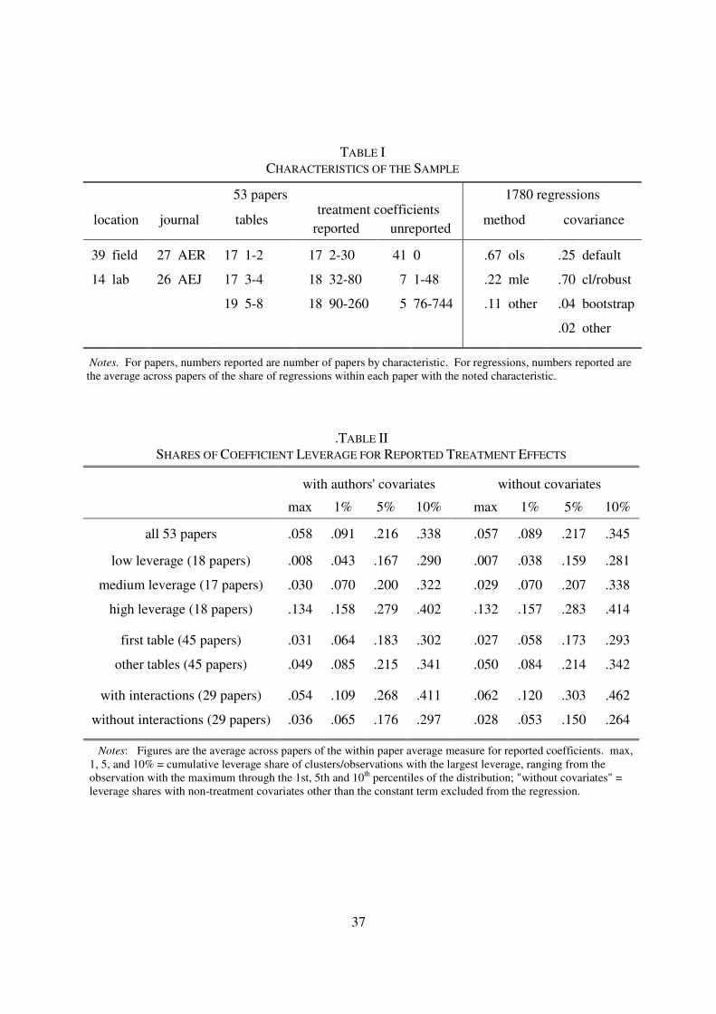
37

TABLE I

CHARACTERISTICS OF THE SAMPLE

53 papers 1780 regressions treatment coefficients

location journal tables reported unreported

method covariance

39

14

field

lab

27

26

AER

AEJ

17

17

19

1-2

3-4

5-8

17

18

18

2-30

32-80

90-260

41

7

5

0

1-48

76-744

.67

.22

.11

ols

mle

other

.25

.70

.04

.02

default

cl/robust

bootstrap

other

Notes. For papers, numbers reported are number of papers by characteristic. For regressions, numbers reported are

the average across papers of the share of regressions within each paper with the noted characteristic.

.TABLE II

SHARES OF COEFFICIENT LEVERAGE FOR REPORTED TREATMENT EFFECTS

with authors' covariates without covariates

max 1% 5% 10% max 1% 5% 10%

all 53 papers .058 .091 .216 .338 .057 .089 .217 .345

low leverage (18 papers)

medium leverage (17 papers)

high leverage (18 papers)

.008

.030

.134

.043

.070

.158

.167

.200

.279

.290

.322

.402

.007

.029

.132

.038

.070

.157

.159

.207

.283

.281

.338

.414

first table (45 papers)

other tables (45 papers)

.031

.049

.064

.085

.183

.215

.302

.341

.027

.050

.058

.084

.173

.214

.293

.342

with interactions (29 papers)

without interactions (29 papers)

.054

.036

.109

.065

.268

.176

.411

.297

.062

.028

.120

.053

.303

.150

.462

.264

Notes: Figures are the average across papers of the within paper average measure for reported coefficients. max,

1, 5, and 10% = cumulative leverage share of clusters/observations with the largest leverage, ranging from the

observation with the maximum through the 1st, 5th and 10th percentiles of the distribution; "without covariates" =

leverage shares with non-treatment covariates other than the constant term excluded from the regression.

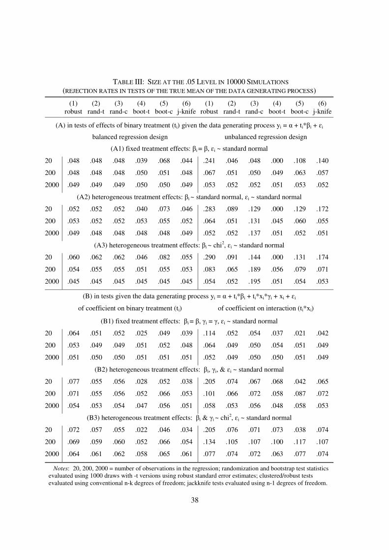
38

TABLE III: SIZE AT THE .05 LEVEL IN 10000 SIMULATIONS

(REJECTION RATES IN TESTS OF THE TRUE MEAN OF THE DATA GENERATING PROCESS)

(1)

robust

(2)

rand-t

(3)

rand-c

(4)

boot-t

(5)

boot-c

(6)

j-knife

(1)

robust

(2)

rand-t

(3)

rand-c

(4)

boot-t

(5)

boot-c

(6)

j-knife

(A) in tests of effects of binary treatment (ti) given the data generating process yi = α + ti*βi + ɛi

balanced regression design unbalanced regression design

(A1) fixed treatment effects: βi = β, ɛi ~ standard normal

20

200

2000

.048

.048

.049

.048

.048

.049

.048

.048

.049

.039

.050

.050

.068

.051

.050

.044

.048

.049

.241

.067

.053

.046

.051

.052

.048

.050

.052

.000

.049

.051

.108

.063

.053

.140

.057

.052

(A2) heterogeneous treatment effects: βi ~ standard normal, ɛi ~ standard normal

20

200

2000

.052

.053

.049

.052

.052

.048

.052

.052

.048

.040

.053

.048

.073

.055

.048

.046

.052

.049

.283

.064

.052

.089

.051

.052

.129

.131

.137

.000

.045

.051

.129

.060

.052

.172

.055

.051

(A3) heterogeneous treatment effects: βi ~ chi2, ɛi ~ standard normal

20

200

2000

.060

.054

.045

.062

.055

.045

.062

.055

.045

.046

.051

.045

.082

.055

.045

.055

.053

.045

.290

.083

.054

.091

.065

.052

.144

.189

.195

.000

.056

.051

.131

.079

.054

.174

.071

.053

(B) in tests given the data generating process yi = α + ti*βi + ti*xi*γi + xi + ɛi

of coefficient on binary treatment (ti) of coefficient on interaction (ti*xi)

(B1) fixed treatment effects: βi = β, γi = γ, ɛi ~ standard normal

20

200

2000

.064

.053

.051

.051

.049

.050

.052

.049

.050

.025

.051

.051

.049

.052

.051

.039

.048

.051

.114

.064

.052

.052

.049

.049

.054

.050

.050

.037

.054

.050

.021

.051

.051

.042

.049

.049

(B2) heterogeneous treatment effects: βi, γi, & ɛi ~ standard normal

20

200

2000

.077

.071

.054

.055

.055

.053

.056

.056

.054

.028

.052

.047

.052

.066

.056

.038

.053

.051

.205

.101

.058

.074

.066

.053

.067

.072

.056

.068

.058

.048

.042

.087

.058

.065

.072

.053

(B3) heterogeneous treatment effects: βi & γi ~ chi2, ɛi ~ standard normal

20

200

2000

.072

.069

.064

.057

.059

.061

.055

.060

.062

.022

.052

.058

.046

.066

.065

.034

.054

.061

.205

.134

.077

.076

.105

.074

.071

.107

.072

.073

.100

.063

.038

.117

.077

.074

.107

.074

Notes: 20, 200, 2000 = number of observations in the regression; randomization and bootstrap test statistics

evaluated using 1000 draws with -t versions using robust standard error estimates; clustered/robust tests

evaluated using conventional n-k degrees of freedom; jackknife tests evaluated using n-1 degrees of freedom.

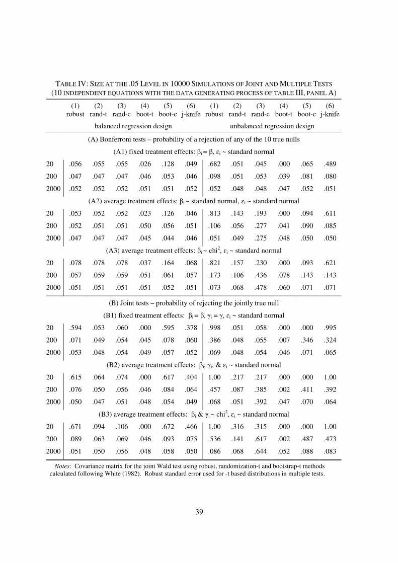
39

TABLE IV: SIZE AT THE .05 LEVEL IN 10000 SIMULATIONS OF JOINT AND MULTIPLE TESTS

(10 INDEPENDENT EQUATIONS WITH THE DATA GENERATING PROCESS OF TABLE III, PANEL A)

(1)

robust

(2)

rand-t

(3)

rand-c

(4)

boot-t

(5)

boot-c

(6)

j-knife

(1)

robust

(2)

rand-t

(3)

rand-c

(4)

boot-t

(5)

boot-c

(6)

j-knife

balanced regression design unbalanced regression design

(A) Bonferroni tests – probability of a rejection of any of the 10 true nulls

(A1) fixed treatment effects: βi = β, ɛi ~ standard normal

20

200

2000

.056

.047

.052

.055

.047

.052

.055

.047

.052

.026

.046

.051

.128

.053

.051

.049

.046

.052

.682

.098

.052

.051

.051

.048

.045

.053

.048

.000

.039

.047

.065

.081

.052

.489

.080

.051

(A2) average treatment effects: βi ~ standard normal, ɛi ~ standard normal

20

200

2000

.053

.052

.047

.052

.051

.047

.052

.051

.047

.023

.050

.045

.126

.056

.044

.046

.051

.046

.813

.106

.051

.143

.056

.049

.193

.277

.275

.000

.041

.048

.094

.090

.050

.611

.085

.050

(A3) average treatment effects: βi ~ chi2, ɛi ~ standard normal

20

200

2000

.078

.057

.051

.078

.059

.051

.078

.059

.051

.037

.051

.051

.164

.061

.052

.068

.057

.051

.821

.173

.073

.157

.106

.068

.230

.436

.478

.000

.078

.060

.093

.143

.071

.621

.143

.071

(B) Joint tests – probability of rejecting the jointly true null

(B1) fixed treatment effects: βi = β, γi = γ, ɛi ~ standard normal

20

200

2000

.594

.071

.053

.053

.049

.048

.060

.054

.054

.000

.045

.049

.595

.078

.057

.378

.060

.052

.998

.386

.069

.051

.048

.048

.058

.055

.054

.000

.007

.046

.000

.346

.071

.995

.324

.065

(B2) average treatment effects: βi, γi, & ɛi ~ standard normal

20

200

2000

.615

.076

.050

.064

.050

.047

.074

.056

.051

.000

.046

.048

.617

.084

.054

.404

.064

.049

1.00

.457

.068

.217

.087

.051

.217

.385

.392

.000

.002

.047

.000

.411

.070

1.00

.392

.064

(B3) average treatment effects: βi & γi ~ chi2, ɛi ~ standard normal

20

200

2000

.671

.089

.051

.094

.063

.050

.106

.069

.056

.000

.046

.048

.672

.093

.058

.466

.075

.050

1.00

.536

.086

.316

.141

.068

.315

.617

.644

.000

.002

.052

.000

.487

.088

1.00

.473

.083

Notes: Covariance matrix for the joint Wald test using robust, randomization-t and bootstrap-t methods

calculated following White (1982). Robust standard error used for -t based distributions in multiple tests.

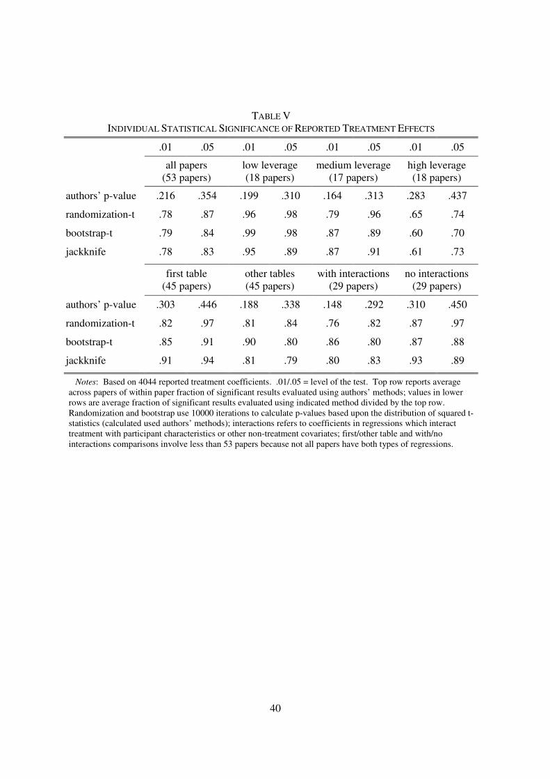
40

TABLE V

INDIVIDUAL STATISTICAL SIGNIFICANCE OF REPORTED TREATMENT EFFECTS

.01 .05 .01 .05 .01 .05 .01 .05

all papers

(53 papers)

low leverage

(18 papers)

medium leverage

(17 papers)

high leverage

(18 papers)

authors’ p-value

randomization-t

bootstrap-t

jackknife

.216

.78

.79

.78

.354

.87

.84

.83

.199

.96

.99

.95

.310

.98

.98

.89

.164

.79

.87

.87

.313

.96

.89

.91

.283

.65

.60

.61

.437

.74

.70

.73

first table

(45 papers)

other tables

(45 papers)

with interactions

(29 papers)

no interactions

(29 papers)

authors’ p-value

randomization-t

bootstrap-t

jackknife

.303

.82

.85

.91

.446

.97

.91

.94

.188

.81

.90

.81

.338

.84

.80

.79

.148

.76

.86

.80

.292

.82

.80

.83

.310

.87

.87

.93

.450

.97

.88

.89

Notes: Based on 4044 reported treatment coefficients. .01/.05 = level of the test. Top row reports average

across papers of within paper fraction of significant results evaluated using authors’ methods; values in lower

rows are average fraction of significant results evaluated using indicated method divided by the top row.

Randomization and bootstrap use 10000 iterations to calculate p-values based upon the distribution of squared t-

statistics (calculated used authors’ methods); interactions refers to coefficients in regressions which interact

treatment with participant characteristics or other non-treatment covariates; first/other table and with/no

interactions comparisons involve less than 53 papers because not all papers have both types of regressions.

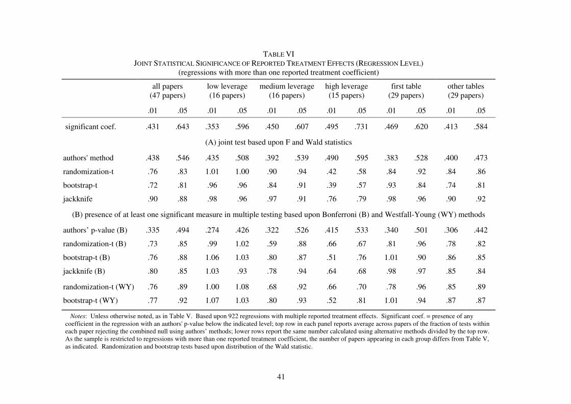
41

TABLE VI

JOINT STATISTICAL SIGNIFICANCE OF REPORTED TREATMENT EFFECTS (REGRESSION LEVEL)

(regressions with more than one reported treatment coefficient)

all papers

(47 papers)

low leverage

(16 papers)

medium leverage

(16 papers)

high leverage

(15 papers)

first table

(29 papers)

other tables

(29 papers)

.01 .05 .01 .05 .01 .05 .01 .05 .01 .05 .01 .05

significant coef. .431 .643 .353 .596 .450 .607 .495 .731 .469 .620 .413 .584

(A) joint test based upon F and Wald statistics

authors' method

randomization-t

bootstrap-t

jackknife

.438

.76

.72

.90

.546

.83

.81

.88

.435

1.01

.96

.98

.508

1.00

.96

.96

.392

.90

.84

.97

.539

.94

.91

.91

.490

.42

.39

.76

.595

.58

.57

.79

.383

.84

.93

.98

.528

.92

.84

.96

.400

.84

.74

.90

.473

.86

.81

.92

(B) presence of at least one significant measure in multiple testing based upon Bonferroni (B) and Westfall-Young (WY) methods

authors’ p-value (B)

randomization-t (B)

bootstrap-t (B)

jackknife (B)

.335

.73

.76

.80

.494

.85

.88

.85

.274

.99

1.06

1.03

.426

1.02

1.03

.93

.322

.59

.80

.78

.526

.88

.87

.94

.415

.66

.51

.64

.533

.67

.76

.68

.340

.81

1.01

.98

.501

.96

.90

.97

.306

.78

.86

.85

.442

.82

.85

.84

randomization-t (WY)

bootstrap-t (WY)

.76

.77

.89

.92

1.00

1.07

1.08

1.03

.68

.80

.92

.93

.66

.52

.70

.81

.78

1.01

.96

.94

.85

.87

.89

.87

Notes: Unless otherwise noted, as in Table V. Based upon 922 regressions with multiple reported treatment effects. Significant coef. = presence of any

coefficient in the regression with an authors' p-value below the indicated level; top row in each panel reports average across papers of the fraction of tests within

each paper rejecting the combined null using authors’ methods; lower rows report the same number calculated using alternative methods divided by the top row.

As the sample is restricted to regressions with more than one reported treatment coefficient, the number of papers appearing in each group differs from Table V,

as indicated. Randomization and bootstrap tests based upon distribution of the Wald statistic.

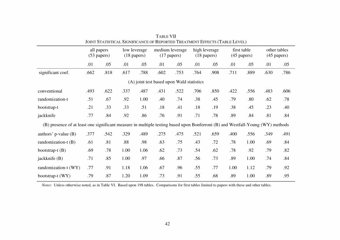
42

TABLE VII

JOINT STATISTICAL SIGNIFICANCE OF REPORTED TREATMENT EFFECTS (TABLE LEVEL)

all papers

(53 papers)

low leverage

(18 papers)

medium leverage

(17 papers)

high leverage

(18 papers)

first table

(45 papers)

other tables

(45 papers)

.01 .05 .01 .05 .01 .05 .01 .05 .01 .05 .01 .05

significant coef. .662 .818 .617 .788 .602 .753 .764 .908 .711 .889 .630 .786

(A) joint test based upon Wald statistics

conventional

randomization-t

bootstrap-t

jackknife

.493

.51

.21

.77

.622

.67

.33

.84

.337

.92

.33

.92

.487

1.00

.51

.86

.431

.40

.18

.76

.522

.74

.41

.91

.706

.38

.18

.71

.850

.45

.19

.78

.422

.79

.38

.89

.556

.80

.45

.84

.483

.62

.23

.81

.606

.78

.40

.84

(B) presence of at least one significant measure in multiple testing based upon Bonferroni (B) and Westfall-Young (WY) methods

authors’ p-value (B)

randomization-t (B)

bootstrap-t (B)

jackknife (B)

.377

.61

.69

.71

.542

.81

.78

.85

.329

.88

1.00

1.00

.489

.98

1.06

.97

.275

.63

.62

.66

.475

.75

.73

.87

.521

.43

.54

.56

.659

.72

.62

.73

.400

.78

.78

.89

.556

1.00

.92

1.00

.349

.69

.79

.74

.491

.84

.82

.84

randomization-t (WY)

bootstrap-t (WY)

.77

.79

.91

.87

1.18

1.20

1.06

1.09

.67

.73

.96

.91

.55

.55

.77

.68

1.00

.89

1.12

1.00

.79

.89

.92

.95

Notes: Unless otherwise noted, as in Table VI. Based upon 198 tables. Comparisons for first tables limited to papers with these and other tables.

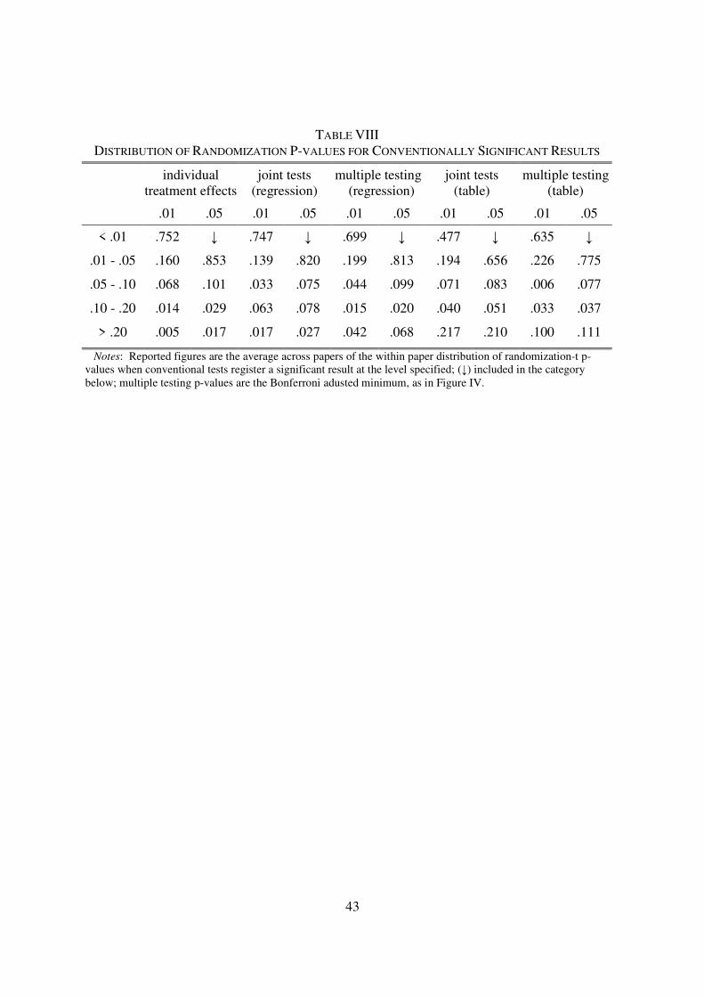
43

TABLE VIII

DISTRIBUTION OF RANDOMIZATION P-VALUES FOR CONVENTIONALLY SIGNIFICANT RESULTS

individual

treatment effects

joint tests

(regression)

multiple testing

(regression)

joint tests

(table)

multiple testing

(table)

.01 .05 .01 .05 .01 .05 .01 .05 .01 .05

< .01

.01 - .05

.05 - .10

.10 - .20

> .20

.752

.160

.068

.014

.005

↓

.853

.101

.029

.017

.747

.139

.033

.063

.017

↓

.820

.075

.078

.027

.699

.199

.044

.015

.042

↓

.813

.099

.020

.068

.477

.194

.071

.040

.217

↓

.656

.083

.051

.210

.635

.226

.006

.033

.100

↓

.775

.077

.037

.111

Notes: Reported figures are the average across papers of the within paper distribution of randomization-t p-

values when conventional tests register a significant result at the level specified; (↓) included in the category

below; multiple testing p-values are the Bonferroni adusted minimum, as in Figure IV.

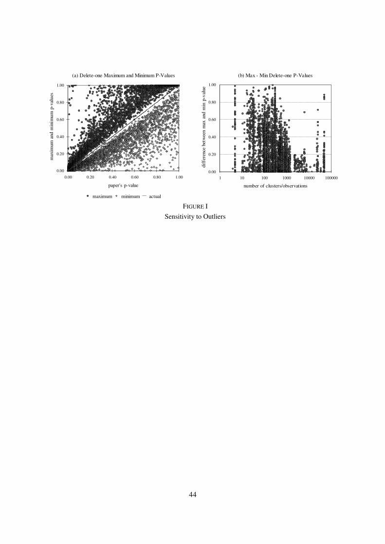
44

0.00 0.20 0.40 0.60 0.80 1.00

paper's p-value

0.00

0.20

0.40

0.60

0.80

1.00

max

imum

and

min

imu

m p

-val

ues

maximum minimum actual

(a) Delete-one Maximum and Minimum P-Values

1 10 100 1000 10000 100000

number of clusters/observations

0.00

0.20

0.40

0.60

0.80

1.00

dif

fere

nce

bet

wee

n m

ax a

nd

min

p-v

alue

(b) Max - Min Delete-one P-Values

FIGURE I

Sensitivity to Outliers

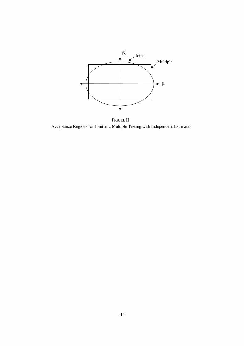
45

β1

β2 Joint

Multiple

FIGURE II

Acceptance Regions for Joint and Multiple Testing with Independent Estimates

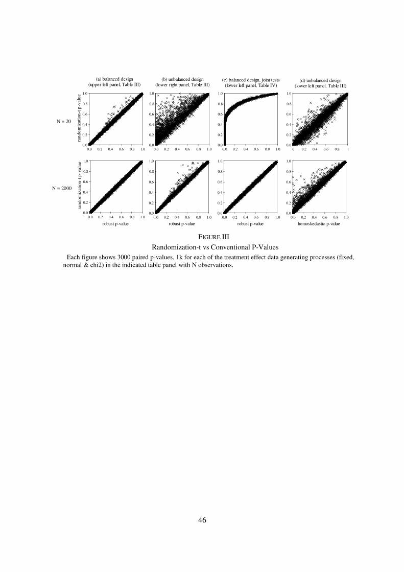
46

N = 20

N = 2000

(a) balanced design(upper left panel, Table III)

(b) unbalanced design(lower right panel, Table III)

(c) balanced design, joint tests(lower left panel, Table IV)

0 0.2 0.4 0.6 0.8 10.0

0.2

0.4

0.6

0.8

1.0

(d) unbalanced design(lower left panel, Table III)

0.0 0.2 0.4 0.6 0.8 1.00.0

0.2

0.4

0.6

0.8

1.0

ran

do

miz

atio

n-t

p-v

alu

e

0.0 0.2 0.4 0.6 0.8 1.0

robust p-value

0.0

0.2

0.4

0.6

0.8

1.0

ran

do

miz

atio

n-t

p-v

alu

e

0.0 0.2 0.4 0.6 0.8 1.00.0

0.2

0.4

0.6

0.8

1.0

0.0 0.2 0.4 0.6 0.8 1.0

robust p-value

0.0

0.2

0.4

0.6

0.8

1.0

0.0 0.2 0.4 0.6 0.8 1.00.0

0.2

0.4

0.6

0.8

1.0

0.0 0.2 0.4 0.6 0.8 1.0

robust p-value

0.0

0.2

0.4

0.6

0.8

1.0

0.0 0.2 0.4 0.6 0.8 1.0

homoskedastic p-value

0.0

0.2

0.4

0.6

0.8

1.0

FIGURE III

Randomization-t vs Conventional P-Values

Each figure shows 3000 paired p-values, 1k for each of the treatment effect data generating processes (fixed,

normal & chi2) in the indicated table panel with N observations.

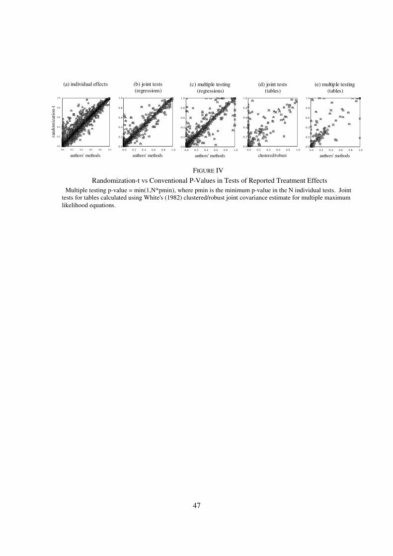
47

0.0 0.2 0.4 0.6 0.8 1.0

authors' methods

0.0

0.2

0.4

0.6

0.8

1.0

ran

dom

izat

ion

-t

(a) individual effects

0.0 0.2 0.4 0.6 0.8 1.0

authors' methods

0.0

0.2

0.4

0.6

0.8

1.0

(b) joint tests

(regressions)

0.0 0.2 0.4 0.6 0.8 1.0

authors' methods

0.0

0.2

0.4

0.6

0.8

1.0

(c) multiple testing

(regressions)

0.0 0.2 0.4 0.6 0.8 1.0

clustered/robust

0.0

0.2

0.4

0.6

0.8

1.0

(d) joint tests

(tables)

0.0 0.2 0.4 0.6 0.8 1.0

authors' methods

0.0

0.2

0.4

0.6

0.8

1.0

(e) multiple testing

(tables)

FIGURE IV

Randomization-t vs Conventional P-Values in Tests of Reported Treatment Effects

Multiple testing p-value = min(1,N*pmin), where pmin is the minimum p-value in the N individual tests. Joint

tests for tables calculated using White's (1982) clustered/robust joint covariance estimate for multiple maximum

likelihood equations.