Channelized Epishelf Lake Drainage Beneath the Milne Ice Shelf, Ellesmere Island,

Nunavut

By

Jill Sophia Thomas Rajewicz

A thesis submitted to the Faculty of Graduate and Postdoctoral Affairs in partial

fulfillment of the requirements for the degree of

Master of Science

In

Geography

Carleton University

Ottawa, Ontario

©2017, Jill Sophia Thomas Rajewicz

ii

Abstract

A depression running across the outer Milne Ice Shelf was hypothesized to overlie a basal

channel incised by outflow from the Milne Fiord epishelf lake, a thick layer of freshwater

impounded in the fiord by the ice shelf. Ice thickness mapping using ice-penetrating radar

revealed the presence of a channel with incision heights of 39 to 45 m (70-80% of mean

ice shelf thickness), basal widths of 57-86 m, and mean sidewall slopes of ~40° upward

from horizontal. Profiles of salinity, temperature and current speed with depth showed

there was a fast flowing jet of epishelf lake water in the channel, with velocities up to 60

cm s-1

, confirming the channel is a drainage outlet for the epishelf lake. The presence of

the channel represents a significant structural weakness along which future breakup of the

ice shelf is likely to occur.

iii

Acknowledgements

This thesis has benefitted from many kinds and sources of support, for which I am

extremely grateful.

Support for this project was provided by a Natural Sciences and Engineering Research

Council of Canada (NSERC) Alexander Graham Bell Canada Graduate Scholarship, a W.

Garfield Weston Award for Northern Research from the Garfield Weston Foundation, the

Ontario Graduate Scholarship from the Ontario Ministry of Training, Colleges and

Universities and scholarships from Carleton University. Research funding also came

from grants from the Northern Scientific Training Program, NSERC, the Polar

Continental Shelf Project, the Canada Foundation for Innovation and ArcticNet.

I owe many, many, many thanks to my supervisor, Dr. Derek Mueller. Derek, thank you

for your patience, guidance, excellent feedback, and sense of humour throughout this

process. I am inspired by your endless curiosity about the world and passion for the work

you do, and I have learned so much about how to do science from you. I am also very

grateful for having had the tremendous opportunity to hone my skills as a field scientist

in one of the most spectacular places on this planet, the northern coast of Ellesmere

Island.

I also owe big thanks to Andrew Hamilton for all his help and advice over the last three

years, not to mention tremendous field ingenuity!

I have had the pleasure of having many excellent field adventures and strange fieldwork

meals with many folks over three field seasons: Kelly Graves, Sam Brenner, Adam

Garbo, Kevin Xu and Greg Crocker, thank you for all your help and for the good times.

Nat Wilson provided advice on ice penetrating radar data interpretation and analysis. Dr.

Chris Burn, my committee member, has given me great advice and support throughout

my whole degree and I appreciate his time and thoughtful comments. My colleagues in

the Water and Ice Research Lab and in the Department of Geography and Environmental

Studies and my wonderful community of friends have also been invaluable sources of

wisdom and support, and have kept me sane and happy!

And last, but most definitely not least, my family have been the best cheerleaders a

person could ask for. Your encouragement and belief in me buoys me and fortifies me.

Thank you for your unflagging love and support, mom, dad, Craig, Lise and Grandma.

Thank you also for inspiring in me a love of learning and a deep appreciation for the

natural world.

iv

Table of Contents

1 Introduction ................................................................................................................. 1

Description of problem......................................................................................... 1 1.1

Research objectives .............................................................................................. 8 1.2

Significance .......................................................................................................... 8 1.3

Thesis structure .................................................................................................... 9 1.4

2 Literature Review...................................................................................................... 10

Ellesmere Island ice shelves ............................................................................... 10 2.1

Epishelf lakes ..................................................................................................... 11 2.2

Ice shelf change .................................................................................................. 13 2.3

Consequences of ice shelf breakup .................................................................... 16 2.4

Causes of ice shelf breakup ................................................................................ 16 2.5

Basal channels .................................................................................................... 18 2.6

Basal channel formation ............................................................................. 18 2.6.1

Channel morphology ................................................................................... 20 2.6.2

Impacts of channelization ........................................................................... 22 2.6.3

Detection and characterization of ice shelf basal channels ......................... 22 2.6.4

Ice penetrating radar ........................................................................................... 23 2.7

Physical principles of ice penetrating radar ................................................ 23 2.7.1

Considerations for IPR data collection and analysis................................... 28 2.7.2

3 Methods..................................................................................................................... 31

Study area ........................................................................................................... 31 3.1

Field campaign overview ................................................................................... 34 3.2

Characterization of feature morphology ............................................................ 35 3.3

Ice thickness surveys................................................................................... 35 3.3.1

Data processing ........................................................................................... 40 3.3.2

Cross-sectional form characterization, measurement and analysis ............. 42 3.3.3

Ice thickness error estimation ............................................................................. 45 3.4

Hydrography....................................................................................................... 48 3.5

Conductivity-temperature-depth profiling .................................................. 48 3.5.1

CTD profile data processing ....................................................................... 50 3.5.2

v

Current velocities ........................................................................................ 50 3.5.3

Estimation of discharge............................................................................... 52 3.5.4

4 Results ....................................................................................................................... 55

Ice thickness survey overview............................................................................ 55 4.1

Channel morphology .......................................................................................... 59 4.2

Comparison of fracture and channel morphology .............................................. 65 4.3

Additional ice thickness measurements ............................................................. 65 4.4

Characterization of snow cover .......................................................................... 68 4.5

Hydrography....................................................................................................... 68 4.6

Temperature and salinity profiles ............................................................... 68 4.6.1

Current measurements ................................................................................ 71 4.6.2

Estimation of discharge............................................................................... 74 4.6.3

5 Discussion ................................................................................................................. 80

Morphological evidence for channelization ....................................................... 80 5.1

Controls on channel surface and basal morphology........................................... 81 5.2

Properties of flow through the channel .............................................................. 87 5.3

Discharge ............................................................................................................ 91 5.4

Fracture hydrography and morphology .............................................................. 93 5.5

Sources of error .................................................................................................. 96 5.6

Implications of channelization for ice shelf stability ......................................... 98 5.7

6 Conclusion .............................................................................................................. 100

7 References ............................................................................................................... 105

Appendix A: Cross-sectional ice thickness profiles from IPR survey grids ................... 116

vi

List of Tables

Table 2.1 Typical values for the electrical properties of common earth materials. Adapted

from Hubbard and Glasser (2005). ................................................................................... 26

Table 3.1 Antenna frequencies and settings for ice penetrating radar surveys of the

channel (grids A-D) and the fracture (grid E). .................................................................. 39

Table 3.2 Summary statistics for a cross-point analysis conducted to assess picking error

in IPR survey data. ............................................................................................................ 46

Table 4.1 Total number of IPR traces recorded and number of traces where the ice-water

reflector could be identified, by survey grid. .................................................................... 58

Table 4.2 Basal and surface morphology metrics calculated from all complete ice

penetrating radar cross-sectional profiles across the channel (grids A to D) and fracture

(grid E). ............................................................................................................................. 61

Table 4.3 Ice thickness and ice draft measurements made through natural cracks and

steam-drilled boreholes in the channel. ............................................................................ 67

Table 4.4 Area, water velocity and discharge for each 1 m depth segment over the

estimated depth of flow in the channel at site 1. Discharge is summed across all segments

for total discharge. ............................................................................................................ 77

Table 4.5 Area, water velocity and discharge for each 1 m depth segment over the

estimated depth of flow in the channel at site 2. Discharge is summed across all segments

for total discharge. ............................................................................................................ 78

vii

List of Figures

Figure 1.1 Maps of the locations and historic and present-day extents of ice shelves in

the Canadian Arctic. Ice shelves are found only along the northwestern coast of

Ellesmere Island, in the Canadian Arctic Archipelago (red box, panel A). Panel B shows

the ice shelf extent as of 2015 in black, and the red arrow indicates the Milne Ice Shelf,

located at the mouth of Milne Fiord. Green shows the greater maximum ice shelf extent-

in 1959, when the ice shelves were first mapped. The approximate extent of the ~8900

km2 ‘Ellesmere Ice Shelf’, reconstructed from observations in the late 1800s/early 1900s,

is shown in blue. White areas are ocean or sea ice; dark grey indicates glaciated areas

(Figure adapted from Mueller et al., 2017a). ...................................................................... 2

Figure 1.2 Schematics of an epishelf lake/ice shelf system (not drawn to scale) in plan

view (A) and side view (B). The floating ice shelf dams terrestrial meltwater in the fiord,

creating a density-stratified epishelf lake wherein freshwater floats on marine water.

When the freshwater layer deepens beyond the minimum draft of the ice shelf, epishelf

lake water flows out beneath the ice shelf to the Arctic Ocean. ......................................... 4

Figure 1.3 RADARSAT-2 Fine Quad image from July 2015 of the outer Milne Ice Shelf

(A) showing the location of the E-W surface depression hypothesized to overlie a basal

channel (red arrow).The blue arrow denotes a fracture formed in 2009 used in this study

to compare morphology and hydrography of a channel and fracture. An older fracture that

dates to at least 1950 can be seen intersecting the E-W depression. Panel B is a photo of

the surface appearance of the fracture. Panel C shows the curvilinear E-W surface

depression with longitudinal crevassing along the margins. Meltwater pools and snow can

be seen in the depression, as well as in surrounding low spots on the ice shelf. An aerial

photo shows the depression in plan view (D); the depression cross-cuts the characteristic

rolling topography of the ice shelf. ..................................................................................... 6

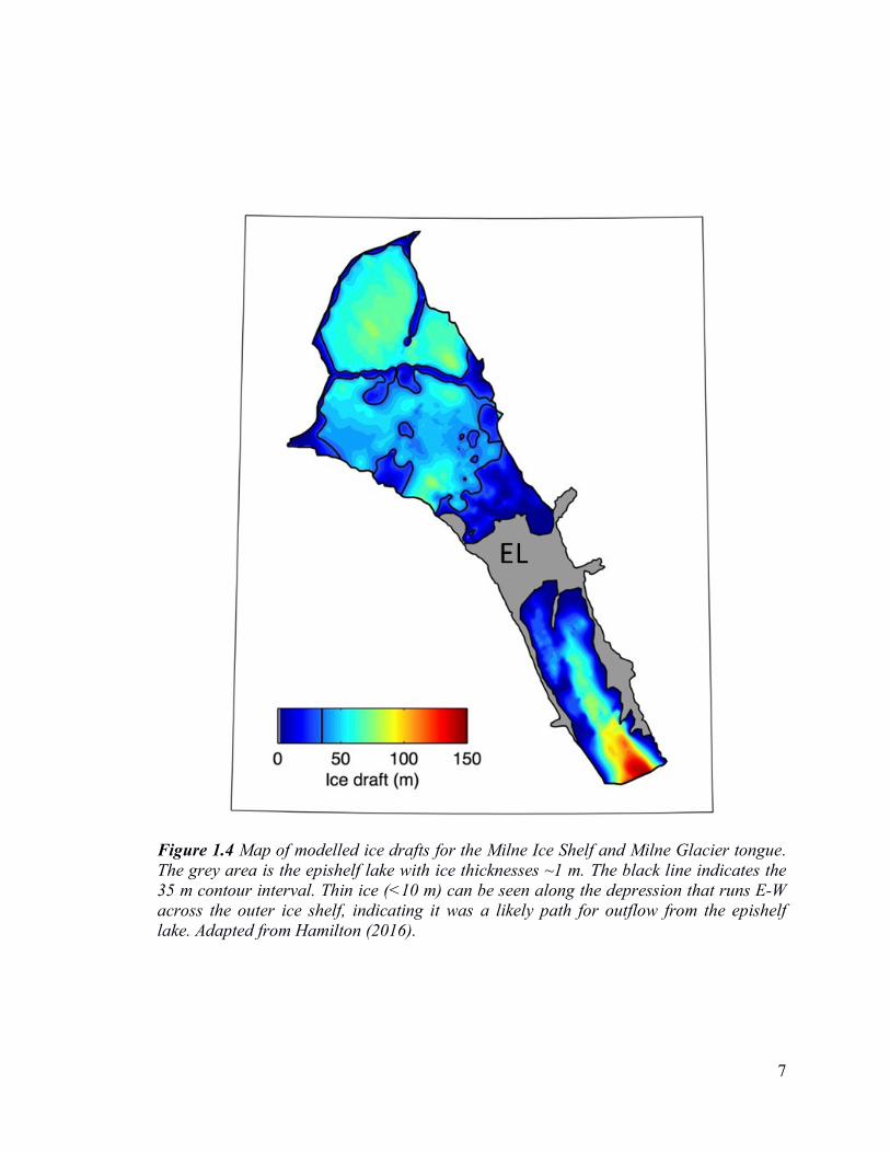
Figure 1.4 Map of modelled ice drafts for the Milne Ice Shelf and Milne Glacier tongue.

The grey area is the epishelf lake with ice thicknesses ~1 m. The black line indicates the

35 m contour interval. Thin ice (<10 m) can be seen along the depression that runs E-W

across the outer ice shelf, indicating it was a likely path for outflow from the epishelf

lake. Adapted from Hamilton (2016). ................................................................................. 7

viii

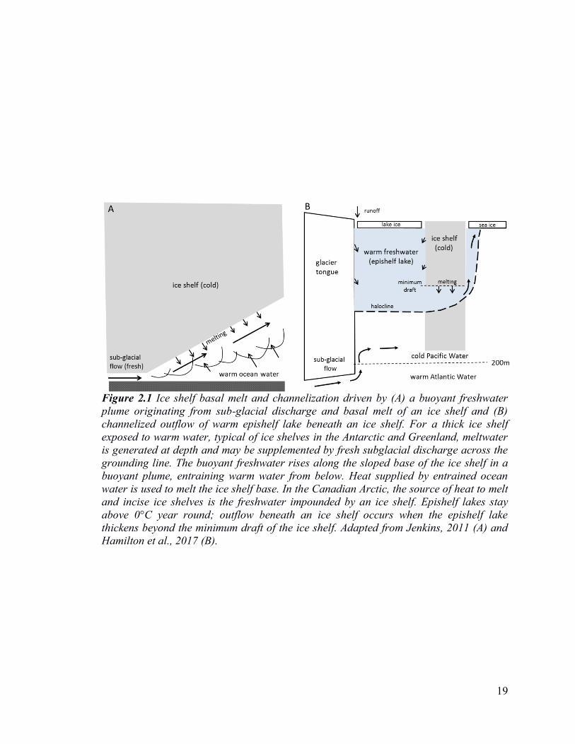
Figure 2.1 Ice shelf basal melt and channelization driven by (A) a buoyant freshwater

plume originating from sub-glacial discharge and basal melt of an ice shelf and (B)

channelized outflow of warm epishelf lake beneath an ice shelf. For a thick ice shelf

exposed to warm water, typical of ice shelves in the Antarctic and Greenland, meltwater

is generated at depth and may be supplemented by fresh subglacial discharge across the

grounding line. The buoyant freshwater rises along the sloped base of the ice shelf in a

buoyant plume, entraining warm water from below. Heat supplied by entrained ocean

water is used to melt the ice shelf base. In the Canadian Arctic, the source of heat to melt

and incise ice shelves is the freshwater impounded by an ice shelf. Epishelf lakes stay

above 0°C year round; outflow beneath an ice shelf occurs when the epishelf lake

thickens beyond the minimum draft of the ice shelf. Adapted from Jenkins, 2011 (A) and

Hamilton et al., 2017 (B). ................................................................................................. 19

Figure 2.2 Ice penetrating radar (IPR) set up: the transmitting antenna sends a pulse of

electromagnetic energy into the ice. When the pulse hits a boundary between materials

with different electrical properties, some of the transmitted energy is reflected back to the

surface. Some of the energy is absorbed and some transmitted into the underlying

substrate. The amplitude and two-way travel time of the reflected pulse is recorded by the

receiver antenna. Two-way travel time can be converted to distance to the reflector, using

the velocity of the radar wave in ice. ................................................................................ 24

Figure 2.3 Configuration of a common-offset survey (A) and the resulting series of radar

traces (B). Pulses are sent and received at regular intervals moving along the direction of

travel. The associated traces show the amplitude and polarity of the transmitted pulse

(airwave and ground wave combined) and the reflected pulse (bed wave). Red dashed

lines indicate the location of the wavelet ‘first break’, which is the first increase in

energy. Two-way travel time to the reflector is calculated using the position of the

airwave first break and bed wave first break. Adapted from Cassidy (2009). .................. 29

Figure 3.1 Map of Milne Fiord on the northern coast of Ellesmere Island, overlaid on an

ASTER image from July 2016. The ice shelf is outlined in black, the epishelf lake is in

orange and a portion of the floating tongue of the Milne Glacier is outlined in green.

Triangles denote the locations of field camps occupied over the years of this study. The

surface depression hypothesized to mark a basal channel is shown with a dashed red line.

ix

A fracture formed between 2008 and 2009 is outlined with a solid blue line. The

hydrography and morphology of the channel and fracture were compared in this study.

Dark blue meltwater ponds can be seen between the rolls on the ice shelf. There are

several other linear features on the outer ice shelf, including a rehealed fracture dating to

at least 1950 that can be seen running N-S from Cape Egerton to intersect the

hypothesized channel. ....................................................................................................... 32

Figure 3.2 Panel A shows the field-ruggedized ice penetrating radar unit (IPR) used in

this study. The transmitter and receiver were ski-mounted, in an in-line, common-offset

survey configuration. The distance between antennae was adjusted as appropriate for the

frequency used for a given survey. A Topcon Hiper V Dual-Frequency GPS receiver unit

was mounted in front of the receiver and recorded precise horizontal positions and

surface elevations along each transect. Panel B shows a survey in progress, with the front

worker pulling the IPR unit and an additional person acting as a brake if required. ........ 36

Figure 3.3 Ice penetrating radar survey grids along the channel (A, B, C and D) and the

fracture (E). Each black line is an IPR transect line. Light green circles indicate the

locations of ice thickness measurements taken in the channel or fracture through natural

cracks or steam-drilled boreholes. Red dashed lines indicate the boundaries between

survey grids. The left and right banks of the channel and fracture show the orientation of

cross channel lines normalized to zero, where zero is the centerline of the feature.

Locations to the left of the centerline have negative values for distance, while locations to

the right of the feature centerline have positive distance values. ..................................... 38

Figure 3.4 Schematics of an idealized channel ice thickness cross-section (A) and an

idealized fracture ice thickness cross-section (B) showing the geometric variables

measured in this study (not to scale). Slope breakpoints indicating the margins of the

feature at the surface and at the ice shelf base are indicated by red dashed lines. For

channel cross-sections, basal incision (‘h’), basal and surface width (‘w’), and the mean

slope angle of each sidewall from horizontal (θ) was calculated. In addition, the thickness

(‘t’) of the ice on the left and right banks was measured, as well as the minimum

thickness of the ice at the crest of the channel. For each fracture cross-section, the

fracture penetration depth (‘d’), minimum thickness of ice within the fracture, width of

the fracture, and slope of the sidewalls up from horizontal was measured. ..................... 44

x

Figure 3.5 Locations of hydrographic measurements in this study. Pink circles indicate

conductivity-temperature-depth (CTD) profiles. CTD profiling was done every year of

the study in the epishelf lake, as well as in three different locations offshore of the

northern edge of the ice shelf. CTD profiling, as well as current measurements were done

at two sites in the channel and at one site in the fracture. Site 1 was at the seaward edge

of the channel; site 2 was further up channel. Current measurements were done with a

point current meter in the channel and an Acoustic Doppler Current Profiler (ADCP) in

the fracture. The ‘u’ axis of the ADCP was oriented along the channel, with positive ‘u’

pointed northeast. The ‘v’ axis was oriented across the fracture, with positive ‘v’ pointed

northwest. .......................................................................................................................... 49

Figure 3.6 Schematic showing how channel cross-sectional geometry was used to

calculate discharge, using the cross section and depth of flow for site 2. The channel was

divided into 1 m horizontal segments over the depth where current measurements were

available. The area of each segment was computed by parameterizing the segment as a

trapezoid. Discharge was calculated for each segment and then summed to get total

discharge through the channel. ......................................................................................... 53

Figure 4.1 Map of point surface elevation measurements along IPR transect grids from a

Dual Frequency GNSS receiver unit post-corrected with Precise Point Positioning. Data

are overlaid on a July 2016 ASTER image of the Milne Ice Shelf. Grids are labelled by

letter on the map and inset boxes, black dashed lines indicate boundaries between grids.

........................................................................................................................................... 56

Figure 4.2 Map of ice thicknesses measured along IPR transect grids. Data are overlaid

on a July 2016 ASTER image of the Milne Ice Shelf from July. Grids are labelled by

letter on map and inset boxes; black dashed lines indicate boundaries between grids. .... 57

Figure 4.3 A radargram from a cross-channel profile in grid D. Multiple radar traces are

aligned side by side in a radargram, in order to show variation in the subsurface over

horizontal space. The continuous black line just below 600 ns is the ice surface. The

bright reflector at 1400 ns is the ice shelf-ocean interface. The channel can be seen in the

ice shelf from trace 45 to 90. On the sides of the channel, there are places where no

reflector can be seen or where identifying the correct reflector was not possible, due to

multiple reflections due to off-nadir reflections from the angled sidewall. ...................... 60

xi

Figure 4.4 Two representative cross-sectional ice thickness profiles (one plotted in green,

one in black) from cross-channel (grids A to D) and cross-fracture (grid E) transects.

Channel profiles run from the left (negative) to right (positive) where the left is defined in

the downstream direction and zero corresponds to the centerline defined along the

channel at the surface of the ice shelf. Fracture profiles run from north (negative) to south

(positive) across the fracture; zero corresponds to the fracture centerline. Plots of channel

and fracture cross-sections not shown here are provided in Appendix A. ........................ 62

Figure 4.5 Boxplots showing variability in mean sidewall slope angle up from horizontal,

calculated for each of the left and right sides of each cross-section, by grid. The right side

of the channel is substantially steeper at grid C, whereas there is no significant difference

in slope angle between the left and right sides for any other grid. The plot for grid E

shows that sidewall slope angles on both sides of the fracture are consistently much

steeper than those of the channel. ..................................................................................... 64

Figure 4.6 Boxplots showing variability in ice thicknesses measured with ice penetrating

radar within the channel (grids A, B, C and D) and within the fracture (E). .................... 66

Figure 4.7 Plots illustrating variability in snow depths measured along grid D IPR

transects. A boxplot of snow depths (A) shows that median snow depth was 0.25 m, with

a minimum of 0.00 and maximum of 2.60 m. A plot of snow depth (B) against distance

from the channel centerline shows that snow depths were most variable in the depression

overlying the channel; peak values were also located in the channel. .............................. 69

Figure 4.8 Temperature and salinity with depth for four locations in an along-channel

CTD transect done in 2015 and 2016. Only the upper water column, to 50 m depth, is

shown. Measurements taken within ice were removed from the top of the profiles and the

downcasts isolated. The solid black line indicates the profile taken offshore of the ice

shelf through a lead in the sea ice; the dashed line is the profile from sampling site 1 at

the seaward edge of the channel; the dotted line is the profile from sampling site 2 located

roughly mid-channel and the solid grey line is the epishelf lake profile for each year. ... 70

Figure 4.9 Salinity and temperature profiles for 2014, 2015 and 2016 showing profiles

from the fracture, plotted against profiles from the epishelf lake and the channel for the

same year for comparison. The channel was not profiled in 2014. For each profile,

measurements taken in ice were removed, and the downcast isolated. The epishelf lake

xii

profile is shown with a solid line, the fracture with a dashed line and the channel profile

with a dotted line. .............................................................................................................. 72

Figure 4.10 Mean water speed with depth at the seaward edge of the channel (site 1), and

approximately mid-way along the channel (site 2). Water speed was measured for 2

minutes at each depth, and the mean of the middle 80% of the recorded values taken.

Mean speed (in m s-1

) is plotted in red; points indicate the depths at which water speed

measurements were recorded. The dashed grey lines indicate one standard deviation from

the mean. Salinity with depth at each location is plotted in blue. ..................................... 73

Figure 4.11 Photos of a weighted line lowered through a natural hole in the ice overlying

the channel. Panel A shows the line before the weight reached the depth of fast flowing

water: the line hung straight down into the water from the hand. Panel B shows the line

when it has been taken up by the fast flowing near-surface current. The line was pulled

downstream (left side of crack in the photo) and thus, angled away from vertical. The red

dashed line marks the vertical from the hand for comparison. ......................................... 75

Figure 4.12 Time-averaged velocities with depth in the water column at the fracture. The

'u' axis is along the fracture, with positive u running NE, toward the intersection of the

fracture and channel. The 'v' axis is oriented roughly along-fiord, with positive v being

toward the ocean. Grey dashed lines indicated one standard deviation from the mean for

each depth. Depth bins are 1.5 m, with the center of the first bin at 2.33 m depth. ......... 76

List of Appendices

Appendix A Cross-sectional ice thickness profiles from IPR survey grids

1

1 Introduction

Description of problem 1.1

The Milne Ice Shelf is one of the few remaining ice shelves in the Canadian Arctic, a

remnant of the vast ‘Ellesmere Ice Shelf’ that once stretched along some 500 km of the

northern coast of Ellesmere Island, Nunavut (Figure 1.1). These ice shelves, thick (>20

m) floating masses of ice attached to land, formed during a period of climatic cooling

4000 – 5500 years ago (England et al. 2008; Antoniades et al., 2011). The course of the

20th

century, however, saw a greater than 90% reduction in ice shelf area; recent years

(since ~2000) in particular have seen accelerated loss as massive calving events and in-

situ fracturing occurred in short succession (Mueller et al., 2003; Copland et al., 2007;

Vincent et al., 2011; Mueller et al., 2017a). Ice shelf decline is understood as a response

to climate change: ice shelf loss is linked with periods of sustained above-average air

temperatures, and a reduction in sea ice coverage along the seaward edge of ice shelves

(e.g. Vincent et al., 2001; Copland et al., 2007; White et al., 2015). Crucial to

understanding past, present and future ice shelf loss, however, is an improved

understanding of the specific mechanisms and processes that link climate warming and

ice shelf break-up.

Studies from Greenland and Antarctica suggest that the nature of the sub-ice shelf

hydrological system plays an important role in ice shelf stability. Basal melt channels

formed by concentrated subglacial outflow plumes or melt-driven cavity circulation have

been identified under many ice shelves and floating glacier tongues in Greenland and

Antarctica (e.g. Rignot and Steffen, 2008; Le Brocq et al., 2013; Langley et al., 2014;

Alley et al. 2016). The presence of basal channels can impact the strength and stability of

2

Figure 1.1 Maps of the locations and historic and present-day extents of ice shelves in

the Canadian Arctic. Ice shelves are found only along the northwestern coast of

Ellesmere Island, in the Canadian Arctic Archipelago (red box, panel A). Panel B shows

the ice shelf extent as of 2015 in black, and the red arrow indicates the Milne Ice Shelf,

located at the mouth of Milne Fiord. Green shows the greater maximum ice shelf extent-

in 1959, when the ice shelves were first mapped. The approximate extent of the ~8900

km2 ‘Ellesmere Ice Shelf’, reconstructed from observations in the late 1800s/early 1900s,

is shown in blue. White areas are ocean or sea ice; dark grey indicates glaciated areas

(Figure adapted from Mueller et al., 2017a).

3

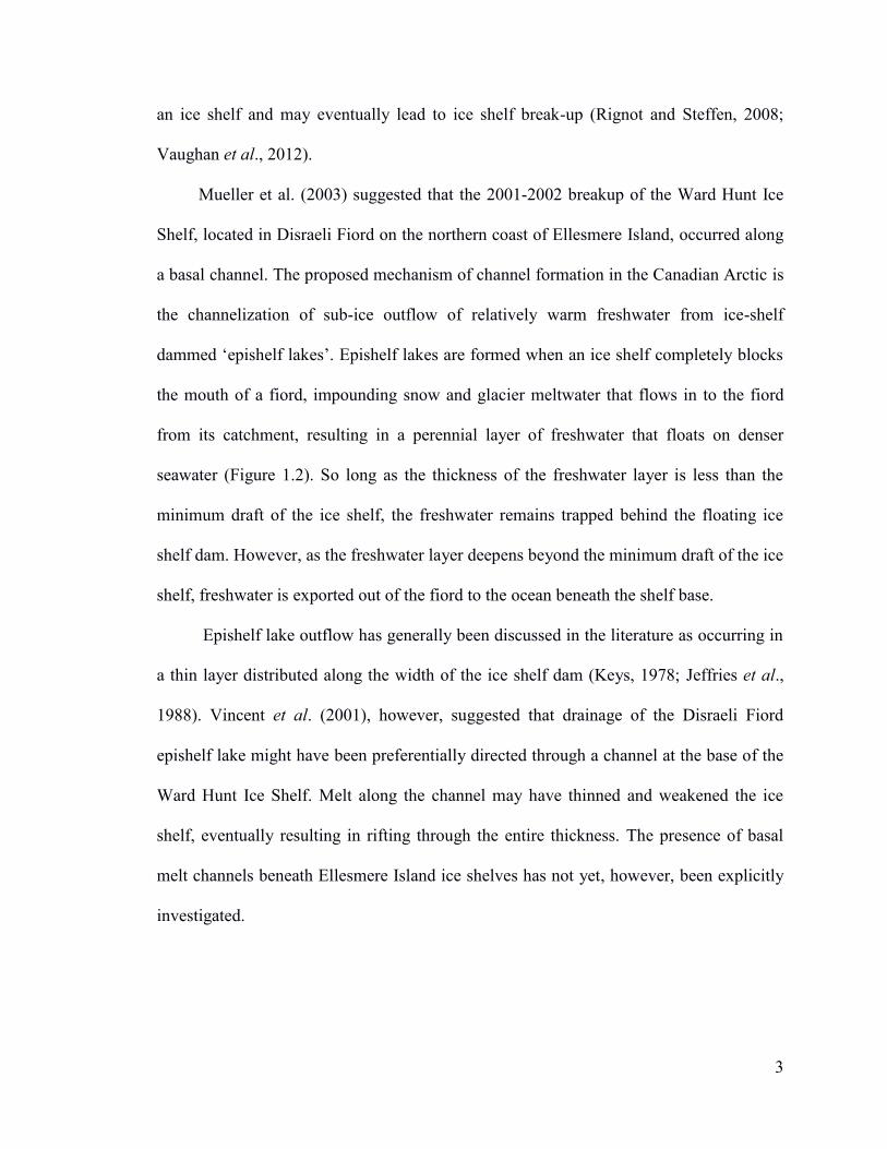
an ice shelf and may eventually lead to ice shelf break-up (Rignot and Steffen, 2008;

Vaughan et al., 2012).

Mueller et al. (2003) suggested that the 2001-2002 breakup of the Ward Hunt Ice

Shelf, located in Disraeli Fiord on the northern coast of Ellesmere Island, occurred along

a basal channel. The proposed mechanism of channel formation in the Canadian Arctic is

the channelization of sub-ice outflow of relatively warm freshwater from ice-shelf

dammed ‘epishelf lakes’. Epishelf lakes are formed when an ice shelf completely blocks

the mouth of a fiord, impounding snow and glacier meltwater that flows in to the fiord

from its catchment, resulting in a perennial layer of freshwater that floats on denser

seawater (Figure 1.2). So long as the thickness of the freshwater layer is less than the

minimum draft of the ice shelf, the freshwater remains trapped behind the floating ice

shelf dam. However, as the freshwater layer deepens beyond the minimum draft of the ice

shelf, freshwater is exported out of the fiord to the ocean beneath the shelf base.

Epishelf lake outflow has generally been discussed in the literature as occurring in

a thin layer distributed along the width of the ice shelf dam (Keys, 1978; Jeffries et al.,

1988). Vincent et al. (2001), however, suggested that drainage of the Disraeli Fiord

epishelf lake might have been preferentially directed through a channel at the base of the

Ward Hunt Ice Shelf. Melt along the channel may have thinned and weakened the ice

shelf, eventually resulting in rifting through the entire thickness. The presence of basal

melt channels beneath Ellesmere Island ice shelves has not yet, however, been explicitly

investigated.

4

Figure 1.2 Schematics of an epishelf lake/ice shelf system (not drawn to scale) in plan

view (A) and side view (B). The floating ice shelf dams terrestrial meltwater in the fiord,

creating a density-stratified epishelf lake wherein freshwater floats on marine water.

When the freshwater layer deepens beyond the minimum draft of the ice shelf, epishelf

lake water flows out beneath the ice shelf to the Arctic Ocean.

5

This study aims to determine whether epishelf lake outflow is channelized beneath the

Milne Ice Shelf. There is a curvilinear surface depression that runs E-W across the

surface of the outer Milne Ice Shelf for 11 km, terminating at the seaward edge of the ice

shelf (Figure 1.3, Panels A, C and D). This feature can be seen in aerial photos dating to

as early as 1950 (Jeffries, 1986). There is evidence to suggest there is a basal channel

incised into the base of the ice shelf beneath this E-W feature.

Previous ice thickness mapping of the ice shelf indicated that ice thicknesses in the

vicinity of the depression were notably less than for other regions of the ice shelf, and

that the most likely path for outflow would therefore be along this E-W feature (Narod et

al., 1988; Mortimer et al., 2012; Hamilton et al., 2017, Figure 1.4). Repeat ice thickness

measurements at one location within the depression showed that ice thickness there

decreased from ~40 m in 1981 to <10 m in 2008/2009 (Mortimer, 2011), which is

broadly consistent with upward incision and the removal of mass from the ice shelf base.

In addition, two cross-sectional profiles of ice thickness across the feature collected

during previous surveys of the ice shelf were suggestive of channelization (Mortimer et

al., 2012; Hamilton, 2016).

The presence of a topographic low on the ice shelf surface is also consistent with

channelization (Luckman et al., 2012; Mankoff et al., 2012); unsupported ice would

deform downward as mass is preferentially removed by channelization. Longitudinal

crevasses were also noted along the margins of the depression (Panel C, Figure 1.3).

Crevassing is consistent with extensional stresses expected where the ice surface sags

downward; similar crevassing is seen as a result of channelization of the Pine Island

Glacier ice shelf in Antarctica (Vaughan et al., 2012).

6

Figure 1.3 RADARSAT-2 Fine Quad image from July 2015 of the outer Milne Ice Shelf

(A) showing the location of the E-W surface depression hypothesized to overlie a basal

channel (red arrow).The blue arrow denotes a fracture formed in 2009 used in this study

to compare morphology and hydrography of a channel and fracture. An older fracture

that dates to at least 1950 can be seen intersecting the E-W depression. Panel B is a

photo of the surface appearance of the fracture. Panel C shows the curvilinear E-W

surface depression with longitudinal crevassing along the margins. Meltwater pools and

snow can be seen in the depression, as well as in surrounding low spots on the ice shelf.

An aerial photo shows the depression in plan view (D); the depression cross-cuts the

characteristic rolling topography of the ice shelf.

7

Figure 1.4 Map of modelled ice drafts for the Milne Ice Shelf and Milne Glacier tongue.

The grey area is the epishelf lake with ice thicknesses ~1 m. The black line indicates the

35 m contour interval. Thin ice (<10 m) can be seen along the depression that runs E-W

across the outer ice shelf, indicating it was a likely path for outflow from the epishelf

lake. Adapted from Hamilton (2016).

8

Research objectives 1.2

This study evaluates the hypothesis that the E-W surface depression on the outer Milne

Ice Shelf overlies a basal channel incised into the ice shelf by outflow from the Milne

Fiord epishelf lake. Accordingly, this study had the following objectives:

1. Characterize the basal morphology of the ice shelf beneath the surface

depression, and compare it to that of a stress fracture that appeared on the ice shelf

between 2008 and 2009 (Figure 1.3, panel B). The morphology of a channel incised by

flowing water will differ from that of a stress fracture due to their different mechanisms

of formation. A channel is expected to have an inverted ‘v’ shape, with sides that slope

away from vertical. A fracture will be straight-sided, with sides closer to vertical.

2. Profile the temperature, salinity and water velocity in the water column

below the feature, and compare these profiles to profiles taken in the epishelf lake, the

fracture, and offshore of the ice shelf, to determine if water properties are consistent with

sub ice-shelf channelized outflow of the epishelf lake water from the fiord.

3. Calculate discharge through the hypothesized drainage channel to

determine whether it might be the primary drainage pathway for the Milne Fiord epishelf

lake, thus gaining a better understanding of the sub-ice shelf hydrology.

Significance 1.3

As a result of ongoing ice shelf break-up along the northern coast of Ellesmere Island,

Milne Ice Shelf dams what is likely the last remaining epishelf lake in the Northern

Hemisphere (Veillette et al., 2008). This work therefore represents the final opportunity

to investigate the presence of basal channels and gain insight into how epishelf lake

drainage may influence ice shelf mass balance and impact ice shelf stability in the

9

Canadian Arctic. Field measurements and observations from this study contribute to our

knowledge of possible mechanisms that determine where, when, and how fractures form

and breakup occurs. An understanding of mechanisms driving present deglaciation also

provides insight into how past deglaciation may have occurred. The applicability of this

study, however, is not limited to the Canadian Arctic. This work in Milne Fiord may also

provide insight into deglaciation in Greenland and Antarctica, as Milne Fiord may

represent a ‘future state’ of ice shelf systems for Greenland and Antarctica. In a warming

climate, it is conceivable that epishelf lakes could develop in the Greenlandic and

Antarctic contexts, if floating ice shelves or glacier tongues become separated from their

glacial trunks but remain attached to the coast.

Thesis structure 1.4

This thesis follows a traditional thesis format. Chapter 2 provides a review of relevant

literature on Ellesmere Island ice shelves and epishelf lakes, ice shelf basal channels, and

ice penetrating radar. The study area and the methods used in this study are described in

Chapter 3. Study results are provided in Chapter 4 followed by a discussion of the

significance of these findings in Chapter 5. Finally, Chapter 6 summarizes the main

conclusions and outlines directions for future work building on this study.

10

2 Literature Review

Ellesmere Island ice shelves 2.1

Ice shelves are best known from Antarctica, where they cover ~40% of the Antarctic

coastline (Drewry et al., 1982). However, ice shelves also occur in northern Greenland,

the Russian High Arctic (Dowdeswell, 2017), and in the Canadian High Arctic in

protected bays and fiords along the northern coast of Ellesmere Island. Where Antarctic,

Greenland and Russian ice shelves are the floating extensions of continental ice, ice

shelves in the Canadian Arctic are both glacial and marine in origin. Ice shelf formation

occurred through in situ surface snow accumulation and basal ice accretion onto

multiyear landfast sea ice (MLSI) and/or glacier ice (Jeffries, 2002). As a result,

Ellesmere Island ice shelves may be classified as sea-ice ice shelves (primarily marine in

origin, e.g. the Ward Hunt Ice Shelf), glacier ice shelves (an ice shelf that has been, or is

still, nourished directly by a glacier, e.g. the Milne Ice Shelf) or composite ice shelves,

having both significant sea ice and glacier ice components (e.g. the Serson Ice Shelf)

(Lemmen et al., 1988). The addition of mass to an ice shelf can also occur via the

accretion of sea ice along the seaward edge of the ice shelf after calving (a ‘reentrant’,

Jeffries, 1986).

Ellesmere Island ice shelves range in thickness from ~20 m to ~100 m (Jeffries,

2002; Mortimer et al., 2012; White et al., 2015). They have a characteristic undulating

surface topography of alternating ridges and troughs (‘rolls’), thought to be formed by the

pattern of snow distribution and elongation of meltwater ponds by the prevailing winds

(Crary, 1960; Jeffries, 1992). Ice shelf mass loss occurs through surface melt and calving

(Jeffries, 2002). Estimates of ice shelf thinning and surface mass balance indicate that

11

basal melt is also likely an important contributor to ice shelf mass loss, but this has not

yet been verified through direct measurements (Braun et al., 2004; Mortimer et al.,

2012). Calving from ice shelves is characterized by the intermittent sudden detachment of

one or more tabular icebergs (‘ice islands’) with an area of many times the ice thickness

(Lazarra et al., 1999). Calving of an ice island is preceded by the formation, propagation

and intersection of fractures that penetrate the entire thickness of the ice shelf (Lazzara et

al., 1999). Calving can occur both at the front of an ice shelf (seaward edge), as well as at

the rear of an ice shelf, into the fiord (c.f. Mortimer et al., 2012). Ice shelves were formed

during a much cooler climatic period and there is no evidence they can reform under

current climatic conditions (Copland et al., 2007).

Epishelf lakes 2.2

Epishelf lakes are formed when terrestrial freshwater is dammed behind a floating ice

shelf. Two types of epishelf lakes have been identified, distinguished by the nature of

their connection with the marine environment (Gibson and Andersen, 2002). The first is

one where the freshwater lake is located on land, and exchange between the freshwater

and ocean occurs indirectly, through a conduit beneath the ice shelf at the ice-land

interface or through cracks in the ice shelf (Gibson and Andersen, 2002). In the second,

the freshwater layer floats directly on seawater and the thickness of the freshwater layer

is controlled by the thickness of the ice shelf dam. It is this type of epishelf lake that has

been identified along the coast of Ellesmere Island, where ice shelves span the mouth of a

fiord or bay (Veillette et al., 2008; Jungblut et al., 2017).

Arctic epishelf lakes are highly stratified, with a well-mixed layer of relatively

warm, fresh to slightly brackish water (absolute salinities of <1.5 g kg-1

, temperatures just

12

above zero to ~4°C) overlying seawater (~30 g kg-1

, <-1ºC) separated by a steep salinity

and temperature gradient (the halocline and thermocline, respectively) (Keys, 1978;

Veillette et al., 2008; Hamilton et al., 2017). The strong and persistent density

stratification is due to a perennial freshwater ice cover on the epishelf lake, which

precludes wind mixing (Keys, 1978; Veillette et al., 2008; Hamilton et al., 2017). Since

there is no physical barrier between the fresh and marine waters, epishelf lakes

experience some tidal exchange. However, the tidal ranges along the coast of Ellesmere

Island are very small (typically <0.20 m between high and low tides, Copland et al.,

2017), so mixing from below is also limited (Veillette et al., 2008). The freshwater layer

is warm because the meltwater runoff that enters the fiord is above freezing, there is little

heat loss to the atmosphere because of a thick insulating snow cover during the winter,

and convective heat loss to the cold ocean below is limited because there is little mixing

at the freshwater-saltwater interface due to strong density stratification (Keys, 1978;

Hamilton, 2016). Solar heating also warms the water near the surface (Veillette et al.,

2008).

The minimum depth of the freshwater layer is approximately equivalent to the

minimum draft of the ice shelf; below this depth, there is free exchange between the fiord

and offshore (Keys, 1978; Vincent et al., 2001; Hamilton et al., 2017). The freshwater

layer deepens over the course of the melt season with meltwater input to the fiord, with

the volume of inflow in a given year dependent on the strength of the melt that year

(Hamilton et al., 2017). When inflow causes an epishelf lake to deepen past the minimum

draft of the ice shelf, water flows out of the fiord beneath the base of the ice shelf, driven

by the difference in density between the buoyant freshwater column and denser seawater

13

(Keys, 1978; Hamilton et al., 2017). Outflow would cease once the depth of the epishelf

lake is equivalent to (or less than) the ice shelf minimum draft.

Epishelf lake outflow could contribute to ice shelf growth, through basal freeze-on

of ice (Keys, 1978; Jeffries and Sackinger, 1988; Jeffries, 1991). Based on measurements

in Disraeli Fiord, Ellesmere Island, Keys (1978) suggested that, as brackish water near

the freezing point flowed from the base of the epishelf lake under the ice shelf, it would

lose heat to the colder seawater below and could form ice crystals or supercooled water

that would subsequently accrete to the base of the ice shelf. Although there have been no

in-situ measurements of sub-ice shelf circulation, ice cores from the Ward Hunt Ice Shelf

suggest basal accretion of epishelf lake water had occurred beneath the Ward Hunt Ice

Shelf (Jeffries and Sackinger, 1988). Keys (1978) theorized that epishelf outflow must

occur in a ‘uniform sheet’ across the width of the ice shelf. He reasoned that if epishelf

lake water flowed out through a channel, the channel would quickly be filled by ice

formed when cooled epishelf lake water came in contact with the ice shelf base and thus,

a consistent ice dam thickness should be maintained by basal accretion (Keys, 1978). The

presence of a deeply incised basal channel in an ice shelf implies that Keys’ model is

perhaps too simplistic, or that channelization is unlikely to be initiated by outflow alone.

Ice shelf change 2.3

Observations from early 20th

century explorations along the northern coast of Ellesmere

by Lieutenant Pelham Aldrich and Commander Robert Peary suggest that there was once

a continuous ice shelf along the northern coast of Ellesmere, with an area of ~8900km2

(Figure 1.1; Vincent et al., 2001). By the early 1950s, however, episodic calving had

significantly reduced the Ellesmere Ice Shelf, leaving several small individual ice shelves

14

in protected bays and fiords (Vincent et al., 2001). From the 1950s to the end of the 20th

century, ice shelves were relatively stable (Mueller et al., 2017a). By the end of the 20th

century, six major ice shelves remained, with a combined area of 1043 km2: the Serson,

Petersen, Ward Hunt, Milne, Markham and Ayles ice shelves (Mueller et al., 2006).

A renewed period of ice shelf loss and breakup occurred from the early 2000s until

2012, which included the loss of the Ayles Ice Shelf in 2005 (Copland et al., 2007), a

60% reduction in area of the Serson Ice Shelf, calving of the entire 50 km2 Markham Ice

Shelf in 2008 (Mueller et al., 2008; Vincent et al., 2009), and ongoing decline of the

Ward Hunt and Petersen ice shelves (Mueller et al., 2017a). The pace of loss has reduced

since 2012 but this is likely a temporary lull (Mueller et al., 2017a). Presently, five major

ice shelves remain (the Serson, Petersen, Ward Hunt, Ward Hunt East and Milne ice

shelves) which represent <6% of the area of the original Ellesmere Ice Shelf (Mueller et

al., 2017a).

Ice shelf loss and disintegration have also resulted in the disappearance of epishelf

lakes, since the existence of an epishelf lake is dependent on an intact ice shelf dam

(Veillette et al., 2008). In 2002, for instance, the fracturing event that bisected the Ward

Hunt Ice Shelf resulted in the drainage of the associated epishelf lake in Disraeli Fiord

(Mueller et al., 2003). Fracturing of the Petersen Ice Shelf in 2005 also resulted in the

drainage of the epishelf lake it dammed (White et al., 2015). At one time, the Ellesmere

Ice Shelf may have dammed up to 17 epishelf lakes (Veillette et al., 2008). As recently as

2007, epishelf lakes were likely still present in five fiords or embayments (Veillette et al.,

2008). At present however, Milne Fiord appears to contain the only remaining deep

epishelf lake in the Arctic (Veillette et al., 2008).

15

The Milne Ice Shelf has suffered less dramatic loss than other ice shelves along the coast

of Ellesmere Island, but nonetheless has decreased in size. Between 1950 and 2009, there

was a 29% reduction in ice shelf area, which amounted to an 82 km2 loss (Mortimer et

al., 2012). One large calving event of 26 km2 occurred sometime between 1959 and 1974

from the northwest corner of the ice shelf (Jeffries, 1986). The ice that calved from the

front was replaced by thinner multiyear landfast sea ice (MLSI) (the Milne ‘re-entrant’ of

Jeffries, 1986). The remainder of the loss occurred through calving at the rear of the ice

shelf and through expansion of ice marginal lakes, causing an expansion of the area of the

epishelf lake (Mortimer et al., 2012; Mueller et al., 2017a). Several new fractures also

developed on the ice shelf between 1981 and 2009 (Mortimer, 2011).

In addition to changes in ice shelf extent, ice shelves in the Canadian Arctic have also

thinned. Thinning occurs when ablation from surface and/or basal melt outpaces

accumulation from surface precipitation, basal accretion, and glacial input. Ablation stake

measurements on the Ward Hunt, Petersen and Milne ice shelves indicate an increasingly

negative surface mass balance as a result of increased temperatures and greater surface

melt (Braun et al., 2004; Mortimer et al., 2012; White et al., 2015). A repeat survey of

historical radio echo sounding measurements of ice thickness on the Milne Ice Shelf by

Mortimer et al. (2012) showed that the ice shelf thinned by an average of 8.1 m from

1981-2009. Observations of a 27% reduction in the depth of the Disraeli Fiord epishelf

lake 1967 to 1999 also suggested the Ward Hunt Ice Shelf thinned over that time, though

thinning did not necessarily occur evenly across the whole ice shelf (Vincent et al.,

2001). As mentioned previously, there is little known about basal melt rates beneath ice

shelves along the coast of Ellesmere Island, so the relative contributions of basal and

16

surface melt to thinning are not well resolved. The loss of epishelf lakes associated with

ice shelves means that the potential for basal accretion, which can add mass to an ice

shelf and offset ablation, is also lost (c.f. Jeffries, 1991).

Consequences of ice shelf breakup 2.4

Ice shelf break-up does not contribute to sea level rise as the ice is already floating

(Jeffries, 2002), but it has other potential consequences. Disintegration can result in the

production of very large tabular icebergs (‘ice islands’). Ice islands that calve from the

Northern Ellesmere ice shelves may drift into the Beaufort or Chukchi seas under the

influence of the Beaufort Gyre, where they present a potential hazard to offshore industry

or shipping (Jeffries, 1992; Mueller et al., 2013). Epishelf lakes provide a unique habitat

wherein marine and freshwater organisms co-exist within the same water column,

stratified by the different habitats that exist at different depths, while meltwater ponds on

the surface of ice shelves are colonized by rare cold-tolerant microbial communities

(Vincent et al., 2000; Veillette et al., 2011; Jungblut et al., 2017). Ice shelf loss results in

a loss of these rare habitats and the organisms that depend on them.

Causes of ice shelf breakup 2.5

The Arctic is warming at nearly twice the rate of the global average temperature (ACIA,

2004). The mean annual Arctic land surface air temperature for 2000-2013 was 1.0°C

higher than the average for 1981-2000 (Overland et al., 2014). Sustained periods of years

where annual positive degree days exceed 200 are linked to increased rates of calving and

break-up events in the Canadian Arctic (Copland et al., 2007). It is likely that long-term

negative surface mass balances and thinning, due to the increase in mean annual

temperatures, result in ‘pre-weakened’ ice shelves that are increasingly vulnerable to

17

various stresses that ultimately cause break-up events (Mortimer et al., 2012; Copland et

al., 2017). The timing of ice shelf calving events also appears to be related to periods of

low sea ice coverage and increased open water along the seaward edges of Ellesmere

Island ice shelves (Copland et al., 2017). Arctic sea ice extent has declined over the

satellite record and the lowest extents in the satellite record have all occurred since the

end of the 20th

century (Stroeve et al., 2012). A sea ice ‘buffer’ along the edges of ice

shelves is important in maintaining ice shelf stability because it provides a physical

barrier that holds the ice shelf in place and protects it from wind, waves and impacts with

pack ice (Copland et al., 2007).

Persistent winds, waves and tides have all been suggested as potential mechanisms

that, coupled with ‘pre-weakening’, may induce stresses large enough to finally cause

fracturing and calving of ice shelves, determining the precise timing of breakup events.

Ocean tides can cause the ice to flex, leading to bending stresses that might enlarge

existing cracks or create new fractures: Holdsworth (1971) suggested that the calving of

the Ward Hunt Ice Shelf in 1961-1962 was the result of an extreme tidal range where low

water fell to 50 cm below its normal value, perhaps combined with a coincident seismic

event. Strong winds blowing across an ice shelf may also exert sufficient stress to induce

fracturing. Strong offshore winds are thought to have been key in triggering calving of

the Ayles Ice Shelf in 2005 (Copland et al., 2007). It has also been proposed that ocean

waves might induce vibrations in the ice which can increase stresses to the point that

fracturing occurs (Holdsworth and Glynn, 1981).

18

Basal channels 2.6

Basal channel formation 2.6.1

The melt rate of an ice shelf by warm water is primarily a function of flow velocity and

thermal driving, which is the difference in temperature between the water and the

freezing temperature at the ice shelf base (Holland et al., 2008). Basal channels form

when warm water beneath an ice shelf somehow becomes concentrated, resulting in

locally higher melt rates and, thus, incision of the ice shelf base (Dutrieux et al., 2013;

Stanton et al., 2013). In Greenland and Antarctica, ice shelf melt is driven by ice shelf

exposure to relatively warm ocean waters at depth, which causes melting at the ice shelf

base. Ice shelves thin away from their grounding lines, resulting in a sloped base.

Meltwater is less dense than seawater, so it rises along the sloped ice shelf base in a

buoyant plume, entraining the warm waters from below as it goes; heat supplied by this

entrained ocean water is used to melt the ice shelf base (Figure 2.1; Jenkins, 1991;

Jenkins, 2011). Additional freshwater may be added by the discharge of subglacial

meltwater across the grounding line of the ice shelf, resulting in even stronger buoyant

plumes (Jenkins, 2011). Several mechanisms have been proposed to explain how the

channelization of warm water is initiated beneath Antarctic and Greenland ice shelves.

Basal channels under some ice shelves may be the result of channelized subglacial

discharge exiting the grounding line of an ice shelf (i.e. channels are an ‘extension’ of the

subglacial hydrological pathways) (Le Brocq et al., 2013). In other cases, it is thought

that variations in ice thickness, caused by topographic features upstream of the grounding

line (Gladish et al., 2012) or variability in lateral shear along ice shelf margins(Sergienko

et al., 2013) are preferentially amplified and deepened by ocean melting via the buoyant

19

Figure 2.1 Ice shelf basal melt and channelization driven by (A) a buoyant freshwater

plume originating from sub-glacial discharge and basal melt of an ice shelf and (B)

channelized outflow of warm epishelf lake beneath an ice shelf. For a thick ice shelf

exposed to warm water, typical of ice shelves in the Antarctic and Greenland, meltwater

is generated at depth and may be supplemented by fresh subglacial discharge across the

grounding line. The buoyant freshwater rises along the sloped base of the ice shelf in a

buoyant plume, entraining warm water from below. Heat supplied by entrained ocean

water is used to melt the ice shelf base. In the Canadian Arctic, the source of heat to melt

and incise ice shelves is the freshwater impounded by an ice shelf. Epishelf lakes stay

above 0°C year round; outflow beneath an ice shelf occurs when the epishelf lake

thickens beyond the minimum draft of the ice shelf. Adapted from Jenkins, 2011 (A) and

Hamilton et al., 2017 (B).

20

plume (Gladish et al., 2012). Regardless of the mechanism of formation, once a channel

is initiated, the buoyant meltwater plume is then preferentially directed into the channel,

resulting in flow speeds and melt rates that are much higher within the channel than out

of the channel (Rignot and Steffen, 2008; Dutrieux et al., 2013).

Beneath the Milne Ice Shelf, entrainment of warm water by buoyant freshwater

plumes is unlikely to be a source of warm water for potential channelization and melt of

the ice shelf base (Figure 2.1). Warm (0-3°C), saline Atlantic Water is found only below

~200 m depth in Milne Fiord, above that is cold, fresh Pacific Water (Hamilton, 2016).

The Milne Ice Shelf is thin enough that it does not float in Atlantic Water, so it is

insulated from this warm layer. While there are also subglacial meltwater plumes

discharged across the grounding line of Milne Glacier that entrain warm water at depth,

these plumes reach their level of neutral buoyancy (the depth at which they no longer rise

through the water column) between 30 and 55 m depth, which is below the halocline

marking the base of epishelf lake (Hamilton, 2016). The sole source of warm water to

drive basal channelization in Milne Fiord is therefore outflow from the epishelf lake. The

epishelf lake represents a significant source of heat to melt ice as it has an elevated heat

content (temperatures >0°C) year round (Hamilton, 2016). Concentration of epishelf lake

outflow in a channel would result in an elevated heat flux from the relatively warm

epishelf lake water to the ice (Hamilton et al., 2017).

Channel morphology 2.6.2

Channels identified under Antarctic and Greenland ice shelves are hundreds of meters to

a few kilometers wide, with heights of many tens to hundreds of meters (Rignot and

Steffen, 2008; Vaughan et al., 2012; Dutrieux et al., 2014). Channel orientations both

21

parallel and perpendicular to the direction of ice flow have been observed (Rignot and

Steffen, 2008; Dutrieux et al., 2014). A surface depression is associated with most

channels, formed by the downward sagging of unsupported ice at the channel crest

(Mankoff et al., 2012; Vaughan et al., 2012). These depressions, however, are often not

as deep as would be expected if the ice was in hydrostatic equilibrium, because of snow

accumulation in the depression or bridging stresses limiting relaxation (e.g. Vaughan et

al., 2012).

Channels have sides that slope away from vertical, but the slope of the channel

sides does not appear to be consistent; reported channel height to width ratios vary

between ice shelves (Rignot and Steffen, 2008; Le Brocq et al., 2013; Langley et al.,

2014). Channel sides have been characterized as smooth by several investigators (Rignot

and Steffen, 2008; Stanton et al., 2013), although Dutrieux et al. (2014) found evidence

of stepped terraces along channel walls on the Petermann Glacier and Pine Island Ice

Shelf. Melting in channels may take place right at the channel apex (Stanton et al., 2013)

or it may be more concentrated along channel sides (Rignot and Steffen, 2008; Dutrieux

et al., 2014), depending on the stratification of the water column in the channel.

Modelling studies also suggest that channel morphology should be asymmetrical, due to

the deflection of flow through a channel by the Coriolis force (Sergienko et al., 2013).

This deflection results in melt concentrated to one side and, thus, a steeper sidewall on

the side because melt is intensified where flow is faster (Gladish et al., 2012; Sergienko

et al., 2013).

22

Impacts of channelization 2.6.3

The presence of basal channels reduces the mechanical strength of an ice shelf, as

concentrated melt causes localized thinning (Rignot and Steffen, 2008). Crevassing at the

base and surface in the vicinity of a channel, due to the generation of extensional stress as

the ice shelf settles back to hydrostatic equilibrium, also reduces the structural integrity of

an ice shelf (Vaughan et al., 2012). While strength is locally reduced along a channel due

to thinning and crevassing, however, the presence of basal channels may in some cases

actually reduce the total amount of melting occurring under an ice shelf. By concentrating

the melting in channels, modelling studies show that the mean melt rate elsewhere is

diminished, which can result in less melting overall than if no channels were present

(Gladish et al. 2012; Millgate et al., 2013).

While this scenario may hold true for Antarctic and Greenland ice shelves, it likely

does not apply in the Ellesmere Island oceanographic context. A thin, distributed layer of

epishelf lake outflow is more likely to result in epishelf lake water quickly losing heat

and freezing on to the ice shelf base, adding mass, not causing additional melt.

Channelized melt would therefore be more likely to destabilize an ice shelf in the

Canadian Arctic, through the combined effects of localized thinning and the loss of a

mechanism to add mass to the ice shelf.

Detection and characterization of ice shelf basal channels 2.6.4

The presence of basal channels beneath ice shelves and floating glacier tongues can be

inferred from the presence of surface depressions seen in satellite imagery (Humbert et

al., 2015; Alley et al., 2016). In some cases, surface topography can yield information

about channel cross-sectional and plan morphology (Alley et al., 2016). However, the

23

degree to which surface topography echoes basal topography depends on many factors,

including the time ice has had to adjust to the removal of mass from the base, bridging

stresses in the ice and the pattern of surface accumulation of mass since the formation of

the depression (Luckman et al., 2012; Humbert et al., 2015). Therefore, to obtain detailed

and accurate information about the morphology and extent of basal channels beneath ice

shelves, it is necessary to image the ice shelf base.

Limited measurements of channel morphology have been obtained through acoustic

radar surveys by autonomous underwater vehicles deployed beneath ice shelves

(Vaughan et al., 2012). Much more common, however, is the use of airborne or ground

penetrating radar for mapping of basal channels (e.g. Rignot and Steffen, 2008; Vaughan

et al., 2012; Langley et al., 2014). Ground penetrating radar uses the transmission and

reflection of radio waves to image the subsurface (Annan, 2009). The application of radar

specifically to the imaging of ice bodies is referred to as ice penetrating radar (IPR).

Identification of the ice-water interface of a floating ice shelf or glacier tongue gives ice

thickness; this is combined with surface elevation measurements to yield a detailed

picture of ice shelf basal topography (Cassidy, 2009). In this study, IPR was used to map

the purported channel incised into the base of the Milne Ice Shelf. A review of important

physical principles and survey considerations for IPR studies follows.

Ice penetrating radar 2.7

Physical principles of ice penetrating radar 2.7.1

An IPR system is composed of a transmitter and a receiver and a pair of antennae in a

fixed geometry (Figure 2.2). The transmitter sends an electrical signal to the transmitting

antenna, which then sends a pulse of radar waves into the ice at regular intervals. Where

24

Figure 2.2 Ice penetrating radar (IPR) set up: the transmitting antenna sends a pulse of

electromagnetic energy into the ice. When the pulse hits a boundary between materials

with different electrical properties, some of the transmitted energy is reflected back to the

surface. Some of the energy is absorbed and some transmitted into the underlying

substrate. The amplitude and two-way travel time of the reflected pulse is recorded by the

receiver antenna. Two-way travel time can be converted to distance to the reflector,

using the velocity of the radar wave in ice.

25

the pulse encounters a boundary between media with different electrical properties (e.g.

travelling from ice to water or ice to air) some of this energy is reflected back up to the

surface, while the rest is either absorbed or penetrates into the underlying material

(Annan, 2009). The amplitude (strength) and travel time of this reflected pulse is

recorded by the receiver antenna at the surface. Two-way travel time can be converted to

depth (and, thus, ice thickness, if the reflector marks the base of the ice mass) by

assuming a velocity for the electromagnetic wave in the ice.

The propagation velocity (V) of a radar wave through ice (or any material) is

controlled primarily by the relative permittivity (Annan, 2009):

𝑉 = 𝑐

√ɛ𝑟

(2.1)

Where c is the speed of light in a vacuum (3.00×108 m s

-1) and ɛr (unitless) is the relative

permittivity of a material, defined as the ratio between the absolute permittivity of the

material to permittivity in a vacuum. Relative permittivity or the ‘dielectric constant’,

describes how easily electromagnetic energy can move through a material (Hubbard and

Glasser, 2005). Permittivity impacts the propagation velocity of a pulse: velocity will be

higher through a material with a low relative permittivity than one with a higher relative

permittivity. Table 2.1 shows the electrical properties of ice and water relative to other

common earth materials. Where a radar wave travels from one material to another, the

amplitude of the reflected wave is a function of the contrast in the relative permittivity of

the two materials (Hubbard and Glasser, 2005). The relative permittivities of ice (3-4)

and water (80) are very different, so IPR works well to identify the location of the ice-

water boundary for floating glacier tongues and ice shelves. Previous studies have

26

Table 2.1 Typical values for the electrical properties of common earth materials.

Adapted from Hubbard and Glasser (2005).

Material Relative electrical permittivity (ɛ

r)

Electrical conductivity (σ, mS m

-1)

Radar wave propagation velocity

(V, ×108 m s

-1)

Air 1 0 3.0

Fresh water 80 0.5 0.33

Ice 3-4 0.01 1.67

Salt water 80 3000 0.1

Granite 4-6 0.01-1 1.3

Silt 5-30 1-100 0.7

27

successfully used IPR to determine the thickness of the Milne Ice Shelf (Narod et al.,

1988; Mortimer et al., 2012).

The strength of a returned radar signal recorded at the surface is also impacted by

factors that cause signal loss within the material. Electrical conductivity describes the

ability of a material to conduct an electric current (Table 2.1, Hubbard and Glasser,

2005). In conductive materials, such as saline ice, the radar signal attenuates (loses

energy) rapidly and will not propagate as deeply (Cassidy, 2009). In contrast, pure ice is a

‘low-loss’ material, meaning there is a low signal loss with depth (Hubbard and Glasser,

2005). Radar signal strength loss also occurs as a result of reflections off heterogeneities

within the ice, which leads to unwanted scatter, termed ‘noise’ or ‘clutter’ (Hubbard and

Glasser, 2005). Scattering loss depends on the size, number and nature of scattering

bodies in the ice, as well as the radar wavelength (Plewes and Hubbard, 2001).

The radar wave that propagates through the ice is a spherical wave, so it also

suffers from attenuation due to geometrical spreading as a result of the spherical

distribution of the energy at the front of the wave (Hubbard and Glasser, 2005). Signal

loss also increases with radar frequency (Annan, 2009). A lower frequency antenna will

therefore result in less attenuation and a deeper signal penetration but will also increase

scattering loss and thus, decrease vertical resolution (Hubbard and Glasser, 2005). The

antenna frequency chosen for a survey should therefore maximize resolution while also

accounting for radar signal loss and ensuring sufficient depth of penetration. Antenna

frequencies of 5 to 1000 MHz are typically used to profile ice, depending on the survey

goals and site characteristics (Hubbard and Glasser, 2005).

28

Considerations for IPR data collection and analysis 2.7.2

A common-offset IPR survey is used to image the subsurface in the horizontal plane

(Annan, 2009). In a common-offset configuration, the transmitter and receiving antenna

are moved together, always separated by a constant distance, which is determined by the

antenna frequency used for the survey (Annan, 2009, Figure 2.3). As the radar system is

moved along the surface, data are recorded as individual radar traces, at regular intervals

along the survey line (Figure 2.3). Traces are plotted as returned signal amplitude (x-axis)

against time (y-axis). Traces can also be plotted side by side to produce a radargram

which shows variation in reflections over space, to assist in interpretation (Hubbard and

Glasser, 2005).

The first (earliest) wavelet seen in a trace is the direct wave, or airwave, which

travelled from the transmitter to the receiver through the air at the speed of light

(Hubbard and Glasser, 2005, Figure 2.3). Then there is the coupled wave, or ground

wave, which travels directly between the transmitter and receiver through the ice, and is

of opposite polarity to the air wave (Arcone et al., 1995). It arrives slightly later, having

travelled through the ice slower than the radar wave in air (Hubbard and Glasser, 2005).

Later returning reflections represent reflections from within the ice and the basal

interface, as well as below the interface until the wave is attenuated. The polarity of the

reflected waves can be used to understand the nature of the reflector and identify the ice

base. A reflected wave passing from a low to high relative permittivity material (e.g. ice

to water, as in the case of a floating ice shelf) will have the same polarity as the air wave

(Arcone et al., 1995). A reversed polarity wave would indicate a transition from a high to

low relative permittivity, e.g. ice to air or water to ice, which could indicate an air or

29

Figure 2.3 Configuration of a common-offset survey (A) and the resulting series of radar

traces (B). Pulses are sent and received at regular intervals moving along the direction

of travel. The associated traces show the amplitude and polarity of the transmitted pulse

(airwave and ground wave combined) and the reflected pulse (bed wave). Red dashed

lines indicate the location of the wavelet ‘first break’, which is the first increase in

energy. Two-way travel time to the reflector is calculated using the position of the

airwave first break and bed wave first break. Adapted from Cassidy (2009).

30

water-filled cavity within the ice. In terms of reflection patterns over space, the simplest

case in an IPR survey is where the base is a planar reflector. However, the spherical

nature of the radar wave means that steeply dipping reflectors in the ice body (such as the

sloping sidewalls of a basal channel, for instance) will cause reflection patterns that

obscure the true nature of the reflector. An angled reflector will result in reflections from

points other than that directly below the radar (the nadir) (Navarro and Eisen, 2010). To

facilitate interpretation, migration can be used in post-processing to move off-nadir

reflectors to their correct spatial position (Fisher et al., 1992).

The vertical resolution of a radar survey (the minimum detectable ice thickness) is

determined by the wavelength of the antenna frequency (Mingo and Flowers, 2010). The

wavelength of a given antenna frequency, λ, is a function of frequency f and the

propagation velocity of the radar signal V:

𝜆 =𝑉

𝑓 (2.2)

Vertical resolution is usually taken to be a minimum of one quarter of the radar

signal’s wavelength, but in practice one half of the wavelength is a better (more

conservative) estimate (Hubbard and Glasser, 2005).

31

3 Methods

Study area 3.1

The 206 km2 Milne Ice Shelf is located within Milne Fiord (82°35’N 80°35’W), between

Cape Evans and Cape Egerton, along the northern coast of Ellesmere Island in the

Canadian Arctic Archipelago (Figure 3.1). Milne Fiord has an average depth of 436 m,

but there is evidence to suggest the seabed rises to within tens of metres of the surface

under the outer region of the ice shelf (Hamilton, 2016). As a result, the ice shelf base

may be grounded in spots (Hamilton, 2016). Seaward of the ice shelf, the sea bed deepens

to greater than 600 m (Hamilton, 2016). The 55 km long, ~4 km wide Milne Glacier

flows into the head of the fiord. The floating glacier tongue is separated from the ice shelf

by the Milne Fiord epishelf lake, but they were once continuous (Mortimer et al., 2012,

Mueller et al., 2017a). The ice shelf is composed of both glacial and sea ice; glaciers

along the fiord walls still provide a small amount of glacial input (Mortimer et al., 2012;

Richer-McCallum, 2015).

Previous studies have determined that the Milne Ice Shelf has a mean thickness of

55 m and a maximum thickness of 94 m (Mortimer et al., 2012, Figure 1.4). Seaward of

the ice shelf, sea ice abutting the ice shelf has a thickness of 1-5 m (Mortimer, 2011). Ice

thicknesses are greatest on the eastern side adjacent to Cape Egerton and thin toward the

ice shelf edge (Jeffries, 1986; Narod et al. 1988; Mortimer et al., 2012). The outer region

of the ice shelf is characterized by rolls oriented parallel to the coastline with an average

wavelength of 200 m and a maximum height from trough bottom to ridge depth of ~7.5

m (Jeffries, 1986). Dark blue areas on the ice shelf in Figure 3.1 are the meltwater ponds

that form in the troughs of these ice shelf rolls every summer.

32

Figure 3.1 Map of Milne Fiord on the northern coast of Ellesmere Island, overlaid on an

ASTER image from July 2016. The ice shelf is outlined in black, the epishelf lake is in

orange and a portion of the floating tongue of the Milne Glacier is outlined in green.

Triangles denote the locations of field camps occupied over the years of this study. The

surface depression hypothesized to mark a basal channel is shown with a dashed red line.

A fracture formed between 2008 and 2009 is outlined with a solid blue line. The

hydrography and morphology of the channel and fracture were compared in this study.

Dark blue meltwater ponds can be seen between the rolls on the ice shelf. There are

several other linear features on the outer ice shelf, including a rehealed fracture dating

to at least 1950 that can be seen running N-S from Cape Egerton to intersect the

hypothesized channel.

33

The surface depression hypothesized to overlie a basal channel is found in this outer

region (dashed red line, Figure 3.1). The curvilinear depression extends for 11 km,

starting on the eastern margin of the ice shelf and extending west to the ice shelf edge.

The morphology and hydrography of the hypothesized channel (hereafter referred to as

‘the channel’) were compared to those of a linear stress-fracture formed in 2009

(hereafter ‘the fracture’), which has since been infilled with ice (solid blue line, Figure

3.1). There are several other linear features on the outer region of the ice shelf, including

a fracture dating to at least 1950 (Jeffries, 1986) that runs N-S from Cape Egerton and

intersects the channel (Figure 3.1).

Fiordward of the E-W depression, the central part of the ice shelf has rolls that are

more irregular in form and orientation, likely due to the influence of glacier inflow onto

the ice shelf (Jeffries, 1986). Ice thicknesses in this region are more variable and thinner

than the outer region (~50 m) (Narod et al., 1988; Mortimer et al., 2012, Figure 1.4).

Notably, there is a very large area of thin ice (20 – 30 m) in the center of the ice shelf,

just south of the hypothesized channel (Mortimer et al., 2012, Figure 4.1).

Milne Ice Shelf dams the 71.2 km2 Milne Fiord epishelf lake (Mueller et al.,

2017b). The lake is perennially covered by thin (<1 m) freshwater ice and is composed of

a main body extending the width of the fiord, with arms that extend along the sides of the

glacier tongue and pockets within the central part of the ice shelf. The epishelf lake is

spatially uniform in depth, and is characterized by a layer of relatively warm, fresh (0-

3ºC, ~0.2 g kg-1

) water at the surface, separated from seawater (< -1ºC, ~30 g kg-1

) by a

sharp halocline only a few meters thick (Hamilton et al., 2017). Seasonally, the lake

deepens during the summer melt season (mid-June to mid-August) with meltwater input,

34

reaching a maximum depth in mid-August (Hamilton et al., 2017). Once inflow ceases,

the lake continues to drain under the ice shelf (Hamilton et al., 2017). The lake reaches

reaching a minimum depth in early June before beginning to refill again when melt

recommences (Hamilton et al., 2017). The epishelf lake warms over the melt season,

peaking in mid-August (Hamilton et al., 2017). Water temperatures in the epishelf lake

gradually decrease over the winter but remain significantly above 0°C all year (Hamilton

et al., 2017). The epishelf lake has thinned over time from ~17.5 m depth when it was

first measured in 1983 to 8.0 m in 2013 and the rate of thinning has increased over time

coincident with increased air temperatures in the region (Hamilton et al., 2017).

From the base of the epishelf lake to 50 m depth, seawater is influenced by

interactions with ice and with subsurface glacier meltwater runoff, resulting in a water

mass that is fresher (20 g kg-1

to 34 g kg -1

) and up to 1ºC warmer than water at

equivalent depths offshore of the ice shelf (‘fiord-modified water’, Hamilton et al., 2017).

Below 50 m depth, water properties in the fiord are consistent with those offshore

(Hamilton et al., 2017). Cold, relatively fresh Pacific Water is found from 50 to ~200 m;

below that is warm and saline Atlantic Water. The tides in the fiord are small, with a

maximum range of 0.31 m (Hamilton et al., 2017).

Field campaign overview 3.2

Fieldwork was conducted from July 12th

to 27th

2014, July 6th

to July 31st 2015, and July

11 to August 1st, 2016. Helicopter-supported fieldwork was conducted from a base camp

at Purple Valley adjacent to Milne Fiord (82°42’N, 81°34’W) (Figure 3.1). Sampling on

the ice shelf was also done from fly-in field camps on the outer ice shelf (adjacent to the

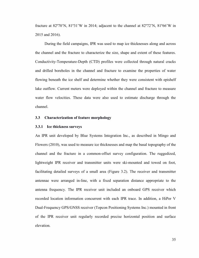
35

fracture at 82º70’N, 81º31’W in 2014; adjacent to the channel at 82º72’N, 81º66’W in

2015 and 2016).

During the field campaigns, IPR was used to map ice thicknesses along and across

the channel and the fracture to characterize the size, shape and extent of these features.

Conductivity-Temperature-Depth (CTD) profiles were collected through natural cracks

and drilled boreholes in the channel and fracture to examine the properties of water

flowing beneath the ice shelf and determine whether they were consistent with epishelf

lake outflow. Current meters were deployed within the channel and fracture to measure

water flow velocities. These data were also used to estimate discharge through the

channel.

Characterization of feature morphology 3.3

Ice thickness surveys 3.3.1

An IPR unit developed by Blue Systems Integration Inc., as described in Mingo and

Flowers (2010), was used to measure ice thicknesses and map the basal topography of the

channel and the fracture in a common-offset survey configuration. The ruggedized,

lightweight IPR receiver and transmitter units were ski-mounted and towed on foot,

facilitating detailed surveys of a small area (Figure 3.2). The receiver and transmitter

antennae were arranged in-line, with a fixed separation distance appropriate to the

antenna frequency. The IPR receiver unit included an onboard GPS receiver which

recorded location information concurrent with each IPR trace. In addition, a HiPer V

Dual-Frequency GPS/GNSS receiver (Topcon Positioning Systems Inc.) mounted in front

of the IPR receiver unit regularly recorded precise horizontal position and surface

elevation.

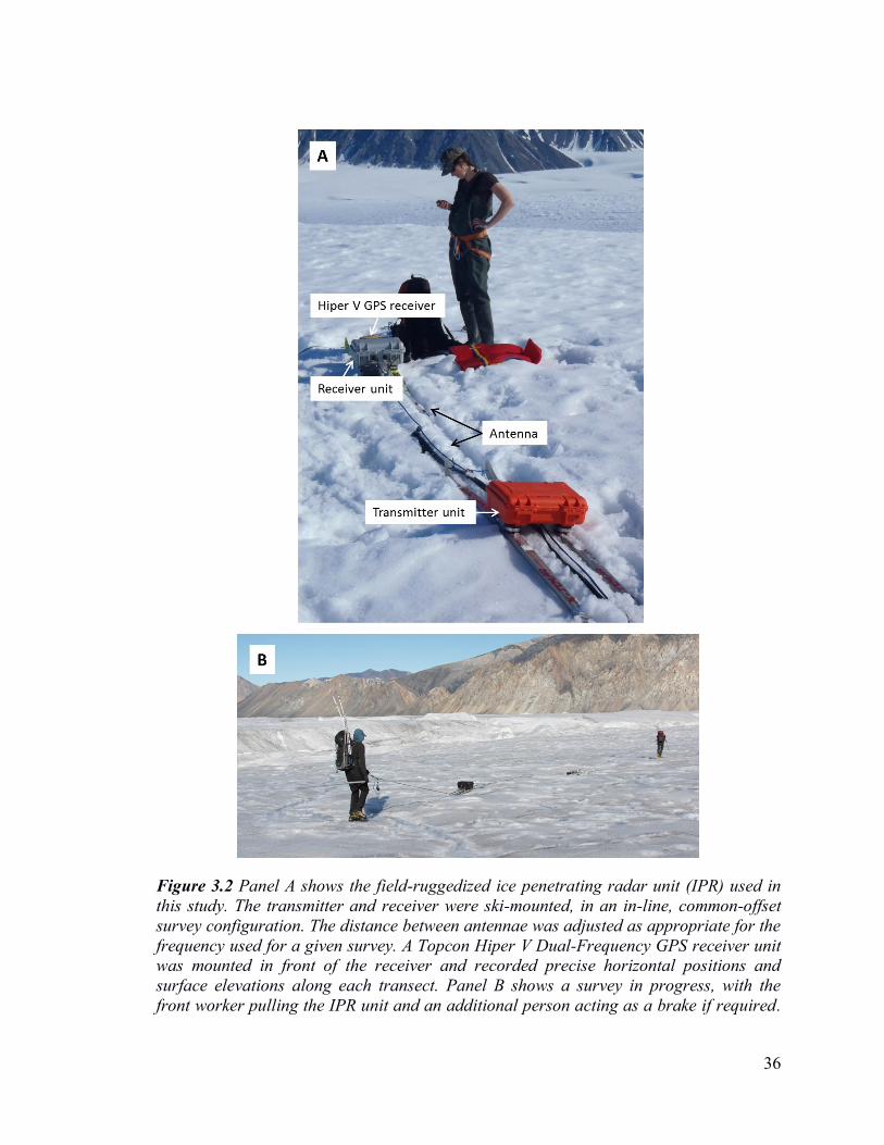
36

Figure 3.2 Panel A shows the field-ruggedized ice penetrating radar unit (IPR) used in

this study. The transmitter and receiver were ski-mounted, in an in-line, common-offset

survey configuration. The distance between antennae was adjusted as appropriate for the

frequency used for a given survey. A Topcon Hiper V Dual-Frequency GPS receiver unit

was mounted in front of the receiver and recorded precise horizontal positions and

surface elevations along each transect. Panel B shows a survey in progress, with the

front worker pulling the IPR unit and an additional person acting as a brake if required.

37

Along- and across-channel IPR profiles were acquired in four survey grids spaced along

the channel in July and August 2014, 2015 and 2016 (grids A, B, C and D, Figure 3.3).

Grid A was located at the seaward edge of the channel. Grids B, C and D were spaced

along the channel with grid D at the far fiordward end of the channel. In 2014, profiles

were taken at the fracture (grid E, Figure 3.3). Survey line locations were limited by

where it was possible to walk back and forth across the channel and fracture; travel was

limited by deep meltwater ponds or slush and by the presence of cracks in the ice

spanning the fracture. Multiple cross-sectional profiles were gathered for each grid, and

the cross-channel or cross-fracture lines extended to at least 100 m on either side of the

channel and fracture.

Both a 50 MHz and 25 MHz antenna were used to image the ice shelf base (Table

3.1). For all surveys, the sampling rate was 2.5×108 samples s

-1. To improve the signal to

noise ratio, each acquired trace was the average of 512 individual traces (stacking)

(Hubbard and Glasser, 2005). The sampling interval of the Hiper V GPS receiver unit

was set to match the IPR sampling interval. For the radar surveys using the 50 MHz

antenna, the minimum detectable thickness (using λ/2) was equal to 1.7 m. For the 25

MHz antenna, it was 3.4 m. Ice thickness measurements were also taken manually

through natural cracks and at boreholes at several locations in the channel and at the

fracture (Figure 3.3).

Snow depth distribution was characterized along several IPR survey lines in grid

D. Depths were measured using an avalanche probe with 5 cm markings along the length

of the probe, at a variable spacing along the transects. It was determined during post-

processing, however, that the temporal and spatial coverage of snow depth measurements

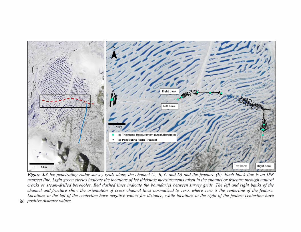
38

Figure 3.3 Ice penetrating radar survey grids along the channel (A, B, C and D) and the fracture (E). Each black line is an IPR

transect line. Light green circles indicate the locations of ice thickness measurements taken in the channel or fracture through natural

cracks or steam-drilled boreholes. Red dashed lines indicate the boundaries between survey grids. The left and right banks of the

channel and fracture show the orientation of cross channel lines normalized to zero, where zero is the centerline of the feature.

Locations to the left of the centerline have negative values for distance, while locations to the right of the feature centerline have

positive distance values.

39

Table 3.1 Antenna frequencies and settings for ice penetrating radar surveys of the

channel (grids A-D) and the fracture (grid E).

Grid Antenna Frequency

(MHz) Antenna Separation

(m) Sampling Interval (s)

A 50 3 10

B 50 & 25 3 & 9 5

C 25 9 5

D 50 3 5

E 50 3 5

40

collected during the field campaign was insufficient to model and subtract snow cover

from the total (snow plus ice) thicknesses recorded with the IPR. Therefore, thicknesses

reported in this document are ice plus snow (if present). The uncertainty in thicknesses

due to snow is discussed in Section 3.4.

Data processing 3.3.2

Positional data recorded by the Hiper V GPS receiver unit were post-processed for

enhanced vertical and horizontal accuracy using the Canadian Spatial Reference System

Precise Point Positioning (PPP) tool from Natural Resources Canada. The horizontal

datum used to reference coordinates was NAD83 and the horizontal datum used to

reference heights was the Canadian Geodetic Vertical Datum of 1928 (CGDV28). After

correction, accuracy for horizontal positions was estimated at ±0.03 m (95%, 2 standard

deviations (SD)). Vertical position accuracy was ±0.07 m (2 SD). Using the Radar Tools

package (Wilson, 2013), readings from the on-board IPR GPS were replaced with the

higher precision PPP-corrected Hiper V GPS positional data by matching time stamps.

PPP-derived elevations and ice thicknesses were corrected for the offset of the

Hiper V GPS receiver unit from the ice shelf surface. Elevations were also corrected for

tidal motion using tidal heights modelled using an 11-month record of water level

collected in Milne Fiord between 01 July 2011 and 01 May 2012 (Hamilton, 2016).

Anomalies from mean sea level were subtracted from surface elevation. The standard

deviation of the residual between observations of tidal height and the model is ±4 cm.

Radar Tools was used to post-process radar data to enhance the bed reflection and

make the identification of the ice-water boundary easier. Stationary radar traces and

empty soundings were removed. A dewow correction was applied to data to remove any

41

very low-frequency signal trend and reduce noise in the data. A linear gain filter was

applied to data where required to enhance later returning reflections and assist in

interpretation. Where required, a Stolt (F-K) migration was used on radargrams to restore

dipping reflectors to their correct spatial positions (Annan, 2009).

The time of the wavelet first break was used as a reference for picking the surface

and reflected waves. Selection of the location of the ice-water interface was done using a

combination of the examination of individual traces; the pattern and spatial relationships

across neighbouring traces; the radargram corrected for surface elevation, and theoretical

ice-thicknesses calculated assuming the ice shelf was in hydrostatic equilibrium. For an

ice shelf in hydrostatic equilibrium, the basal topography should roughly mirror surface

topography. Therefore, in instances where there were multiple strong reflectors at the

same location but different times, the theoretical ice thickness was used as a guide to

selecting the correct reflector (i.e. to determine whether the shallower or deeper reflector

should be selected). In cases where the bed reflection was uncertain or the data were too

noisy to clearly determine the bed reflection, no pick was made.

Once the surface and basal reflectors had been picked wherever possible in all

radargrams, two-way travel time associated with each pick was converted to ice thickness

in metres using the equation:

𝑇(𝑚) = √((𝑡 + (

𝑠0.3)) ⋅ 𝑣

2)

2

−𝑠2

4 (3.1)

where t is two-way travel time in ns, v is the radar wave propagation velocity and s is the

transmitter-receiver antenna separation. According to the literature, the average velocity

of a radar wave through ice is 1.67×108 m s

-1, with slightly higher values for cold, dry ice

42

and slightly lower values for warm, temperate ice (Hubbard and Glasser, 2005). Previous

studies on Ellesmere Island ice shelves have calculated a propagation velocity of 1.7×108

m s-1

(Mortimer et al., 2012) and 1.76×108 m s

-1 (Narod et al., 1988). The velocity

calculated by Narod et al. (1988), however, accounts for propagation through both ice

and firn, through which radar wave velocities may be significantly faster (Clark and

Bentley, 1994). Therefore, a radar wave propagation speed of 1.70×108 m s

-1 was used to

convert measured two-way travel time to ice thickness for this study.

Cross-sectional form characterization, measurement and analysis 3.3.3

Cross-sectional ice thickness profiles were isolated and used to characterize channel and

fracture geometry. Cross-sectional lines that were angled across the channel were

corrected to perpendicular, to correct for any distortion of shape or measurements

resulting from non-perpendicularity. Correction was done as follows: the centerline of the

depression and fracture were digitized, based on the surface appearance of the features in

RADARSAT-2 Fine Quad Mode images (pixel size 6.71 m) from the survey years. Then,

straight lines perpendicular to the channel were defined for each location where an IPR

line crossed the centreline, and the actual radar survey locations projected onto these

lines. Cross-sections were normalized to the centerline, such that measurements to the left

and right of the centerline were defined in terms of horizontal distance from the

centerline (Figure 3.3). For the channel, the left bank (negative distances from 0) was

defined looking in the down-channel (seaward) direction. For the fracture, the left bank

was on the west (seaward) side of the fracture. Margins were defined both for the surface

expression of the feature (elevation > 0 m asl) and for the basal expression (draft below 0

43

m asl), using the slope breaks along the base and the surface of the ice shelf (c.f. Rignot

and Steffen, 2008).

Geometric variables measured for each corrected channel cross-section were:

maximum basal width, maximum incision height, minimum measured ice thickness

within the channel/fracture, upward slope of the sides from horizontal, ice thicknesses of

the left and right banks, and the width and depth of the surface depression (Figure 3.4).

For fracture cross sections, the penetration depth, minimum ice thickness, fracture width

and the slope of the sidewalls from horizontal were measured (Figure 3.4). Summary

statistics were calculated for all measured channel variables over each survey grid. The

channel sidewalls were defined using the basal slope breaks and slope breaks identified at

the crest of the channel. Angles for the left and right sides of the channel were calculated

separately. Missing thicknesses were interpolated for every meter along the channel using

a linear interpolation. Working from the channel margins to the center, the rise and run of

each successive 1 m segment was calculated. This allowed for an examination of

variability in slope along the channel walls. For each cross section, summary statistics

were calculated for the individual slope segments, for each of the left and right sides. The

mean sidewall slope angles reported here for each grid are the mean of the each cross-

section mean slope; the standard deviation is the mean of the standard deviations for each

cross-section.

To examine changes in surface and basal morphology between channel survey

locations, variables were compared between channel survey grids. Differences in basal

widths, surface widths, channel incision heights and mean slope of the channel walls

between channel grids were assessed with a non-parametric Kruskal-Wallis rank sum

44

Figure 3.4 Schematics of an idealized channel ice thickness cross-section (A) and an

idealized fracture ice thickness cross-section (B) showing the geometric variables

measured in this study (not to scale). Slope breakpoints indicating the margins of the

feature at the surface and at the ice shelf base are indicated by red dashed lines. For

channel cross-sections, basal incision (‘h’), basal and surface width (‘w’), and the mean

slope angle of each sidewall from horizontal (θ) was calculated. In addition, the

thickness (‘t’) of the ice on the left and right banks was measured, as well as the

minimum thickness of the ice at the crest of the channel. For each fracture cross-section,

the fracture penetration depth (‘d’), minimum thickness of ice within the fracture, width

of the fracture, and slope of the sidewalls up from horizontal was measured.

45

test. A post-hoc Neyemi pairwise comparison test was done to determine where

differences occurred between groups. Differences in left and right bank thicknesses were

tested for significance using a Wilcoxon rank sum test. A Student’s t-test was used to

assess whether there was a difference in mean slope on the left and right sides of the

channel, within each grid. To compare channel and fracture morphology, the mean slope

of the channel walls was compared to that of the fracture walls, to assess the hypothesis

that the channel would have an inverted ‘v’ shape with sides that slope away from

vertical while fracture sides would be near vertical. Variability in ice thickness within the

channel was also compared with that of the fracture.

Ice thickness error estimation 3.4

There are several sources of measurement uncertainty that must be considered when

determining the accuracy of ice thickness measurements reported here. Uncertainty in

thickness measurements arises from uncertainty in the position of the surface and

reflected waves, which in turn impacts the measurement of the waveform sampling

interval and thus, the two-way travel time and calculated depth. Based on the sampling

rate and radar wave velocity used in this study, the system uncertainty in thickness for

this study is ±0.68 m.

Uncertainty in thickness estimates also arises from operator error in picking the

location of the reflected wave. To assess the impact of magnitude of picking errors, a

cross-point analysis was conducted: all points from independent survey lines that were

within a 4 m radius of each other were identified, and the difference in ice thickness

between each pair of points was calculated. A total of 88 cross-points were identified.

The median picking error from the cross-point analysis was 1.4 m (Table 3.2), with an

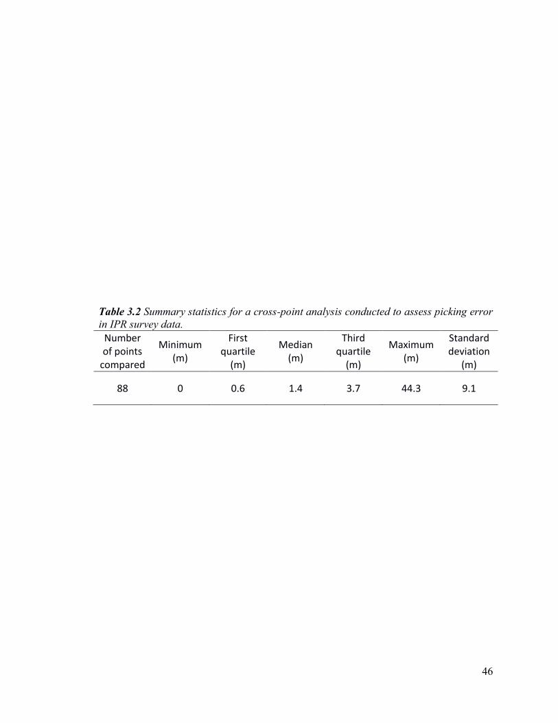
46

Table 3.2 Summary statistics for a cross-point analysis conducted to assess picking error

in IPR survey data.

Number of points

compared

Minimum (m)

First quartile

(m)

Median (m)

Third quartile

(m)

Maximum (m)

Standard deviation

(m)

88 0 0.6 1.4 3.7 44.3 9.1

47

interquartile range of 3.1 m. Summing system uncertainty and the median uncertainty

arising from errors in reflection picking, the uncertainty associated with ice thickness

measurements in this study is ±2.08 m.

There is also uncertainty in the reported thicknesses that result from neglecting the

effect of differential radar wave propagation velocities through snow and through ice. As

previously described, insufficient snow depth measurements collected during the field

campaigns meant it was not possible to estimate or model snow cover on the ice shelf. It

was also not possible to resolve the snow-ice boundary in the radar traces. Therefore,

snow and ice were treated as one, and a radar propagation velocity of 1.70 x 108 m s

-1 was

used to convert two-way travel time to depth for the entire thickness measured.

However, the propagation velocity in snow is faster than in ice (Plewes and

Hubbard, 2001). Thickness calculated from a two-way travel time measured by the IPR

using the propagation velocity of a radar wave in ice would be less than if the faster

velocity for snow were used. The maximum snow depth measured along the IPR transect

was 2.6 m. Using a snow depth of 3 m, the difference in thickness when using a radar

wave velocity in snow of 2.00×108 m s

-1 (c.f. White et al., 2015) to account for the snow

thickness, compared with using only the velocity in ice of 1.70×108 m s

-1, is 0.5 m.

Therefore, by assuming the entire column is ice, the thicknesses reported here may

underestimate thickness by up to ~0.5 m in places where there was appreciable snow. A

very conservative estimate of uncertainty in ice thickness measurements in this study is

then total uncertainty as calculated above, plus 0.5 m due to snow, for a total of ±2.58 m.

48

Hydrography 3.5

Conductivity-temperature-depth profiling 3.5.1

Conductivity-temperature-depth (CTD) profiles were collected to examine the structure

of the water column. Profiles were collected through leads in the sea ice offshore of the

ice shelf and through boreholes and natural cracks through the ice shelf and epishelf lake

ice. Profiling locations were accessed by foot or helicopter. Profiles were taken at two

locations within the channel in 2015 and in 2016, to enable examination of change in

water properties along the channel (sites 1 and 2, Figure 3.5). Profiles were taken at the

fracture in all three years of the study. Profiles were also collected in the epishelf lake

and offshore of the ice shelf, to enable comparison of the water column structure at these

locations with those of the channel and fracture (Figure 3.5).

The profiles were recorded using a 6 Hz XR-620 CTD (RBR-Global Ltd.) and an

8 Hz Ocean Seven 304 Plus CTD (OS 304Plus, Idronaut S.r.l.). At each sampling site,

CTDs were left to equilibrate for at least 1 minute in the water, and lowered through the

water column at a rate of ~0.5 m s-1

. CTD casts were full depth, to the bottom of the

fiord. However, it is the near-surface water column that is of interest here, so only the top

50 m of the profiles are presented herein. The temperature sensor of the OS 304Plus has

an accuracy of ±0.002ºC with a resolution of 0.0001ºC. The pressure sensor accuracy is

±0.05% F.S. (full scale) with a resolution of 0.0015% F.S. and conductivity

measurements are accurate to ±0.003 mS cm-1

with an instrument resolution of 0.0003

mS cm-1

. For the RBR XR-620, the accuracy of the temperature sensor is ±0.002ºC with

a resolution better than 0.00005ºC. Conductivity is accurate to 0.003 mS cm-1

with a

49

Figure 3.5 Locations of hydrographic measurements in this study. Pink circles indicate

conductivity-temperature-depth (CTD) profiles. CTD profiling was done every year of the

study in the epishelf lake, as well as in three different locations offshore of the northern

edge of the ice shelf. CTD profiling, as well as current measurements were done at two

sites in the channel and at one site in the fracture. Site 1 was at the seaward edge of the

channel; site 2 was further up channel. Current measurements were done with a point

current meter in the channel and an Acoustic Doppler Current Profiler (ADCP) in the

fracture. The ‘u’ axis of the ADCP was oriented along the channel, with positive ‘u’

pointed northeast. The ‘v’ axis was oriented across the fracture, with positive ‘v’ pointed

northwest.

50

resolution of 0.0005 mS cm-1

. The accuracy of the pressure sensor on the XR-620 is

better than ±0.05% F.S

CTD profile data processing 3.5.2

For each profile, the downcast was isolated and any measurements taken within ice (e.g.

in a borehole and so not exposed to the ambient water column) were removed. Instrument

pressures were corrected for atmospheric pressure. Further processing and plotting were

done in R using the oce package (Kelley and Richards, 2016): pressures were converted

to depth, and the square of the Brunt-Vӓisӓlӓ buoyancy frequency, N2, was calculated as a

measure of water column stratification. Additionally, Absolute Salinity (SA, g kg-1

) and

Conservative Temperature (Θ, ºC) were derived from Practical Salinity and in-situ

temperature using the Gibbs Seawater TEOS-10 formulation (McDougall and Barker,

2011). As per Hamilton et al. (2017), the depth of the epishelf lake was defined as the

depth of the stratification maximum (maximum N2). Absolute Salinity and Conservative

Temperature were plotted against depth to examine the structure of the water column at

each profile location.

Current velocities 3.5.3

3.5.3.1 Channel measurements

Water speed with depth in the water column was measured in the channel using an

Infinity AEM-USB electromagnetic point current meter (JFE Advantek Co. Ltd) with a

resolution of 0.02 cm s-1

and accuracy of ±1 cm s-1

. Current profiling was done at the

same sampling locations in the channel as the CTD profiles (Figure 3.5). To profile, the

current meter was attached to a line above one of the CTD instruments and the

instruments were lowered in increments through the water column, to a depth of at least

51

25 m. Current speed was recorded for 2 minutes at each depth sampled. The sampling

rate for all profiles with the current meter was 10 Hz.

For analysis, current meter data were matched with the CTD to obtain the exact

depth associated with water speed measurements. First, the CTD data were adjusted for

atmospheric pressure and for the offset between the pressure sensor and current meter.

Due to the difference in sampling rates between the instruments, data from both

instruments were averaged to one second intervals. Then, current speed and depth

measurements were matched by time stamp. The first and last 20% of the current speed

measurements recorded at each depth bin were removed to eliminate the possibility of

readings taken while the instrument was being lowered into or out of position. This issue

was due to a loss of synchrony between times recorded by the CTD, the current meter,

and in field notes. The remaining values were averaged to obtain a mean current speed

for each depth bin. Two profiles were completed at site 2, one after the other and current

speed was recorded at slightly different depths in both profiles. To improve the depth

resolution for current speed, the two profiles were merged.

3.5.3.2 Fracture

Water velocity with depth was measured in the fracture using a 4-beam 300 kHz Sentinel

V100 Acoustic Doppler Current Profiler (ADCP, Teledyne Rd Instruments, Inc). ADCPs

are used to measure current velocity throughout a column of water, providing a time

series of flow over a series of binned depths. The ADCP was installed with a fixed

orientation and deployed looking downward through the water column. The instrument

transducers sat at a depth of 0.6 metres below the water surface. Measurement took place

over 34 hours starting in the morning of July 14th, 2014. The ADCP bin size was 1.5 m,

52

with the center of the first bin at 2.33 m and the last at 100 m. The ADCP recorded an

ensemble at 10 minute intervals, with 100 pings per ensemble at a rate of one ping per

second. The instrument velocity measurement accuracy is ±0.5% of the water velocity

relative to the ADCP, ±0.5 cm s-1. Velocity resolution is 0.1 cm s-1.

ADCP data were processed using the ‘oce’ package in R. Coordinates were

transformed from beam coordinates to instrument (xyz) coordinates. The ‘u’ axis was

oriented along the fracture, roughly cross-fiord with positive u pointed north, and the ‘v’

axis was oriented across the fracture, with positive v pointed west, down-fiord (Figure

3.5). Data were screened for accuracy using a correlation threshold of 64 and for returned

signal strength using an echo intensity threshold of 40 (RD Instruments, 2011). Data were

also screened for consistency in the velocity measurements; any velocities with an

associated error velocity greater than 2 m s-1 were rejected (RD Instruments, 2011).

Finally, an ensemble mean velocity was calculated for each sampling interval from

individual ping measurements. Mean velocity over the entire sampling period was plotted

for each depth bin, for both the u and v axes, to examine velocity with depth at the

fracture site in both the along-fracture and along-fiord directions.

Estimation of discharge 3.5.4

The geometry of the cross-sectional ice thickness profiles closest to each of sampling

sites 1 and 2 were used to calculate the cross-sectional area of the channel over which

flow occurred. For each site, the channel cross-section was divided into 1 m horizontal

segments over the depth range of measurements made with the current meter; an example

for site 2 is shown in Figure 3.6. For each segment where a current velocity measurement

had been made within the depth range encompassed by that segment, that velocity value

53

.

Figure 3.6 Schematic showing how channel cross-sectional geometry was used to

calculate discharge, using the cross section and depth of flow for site 2. The channel was

divided into 1 m horizontal segments over the depth where current measurements were

available. The area of each segment was computed by parameterizing the segment as a

trapezoid. Discharge was calculated for each segment and then summed to get total

discharge through the channel.

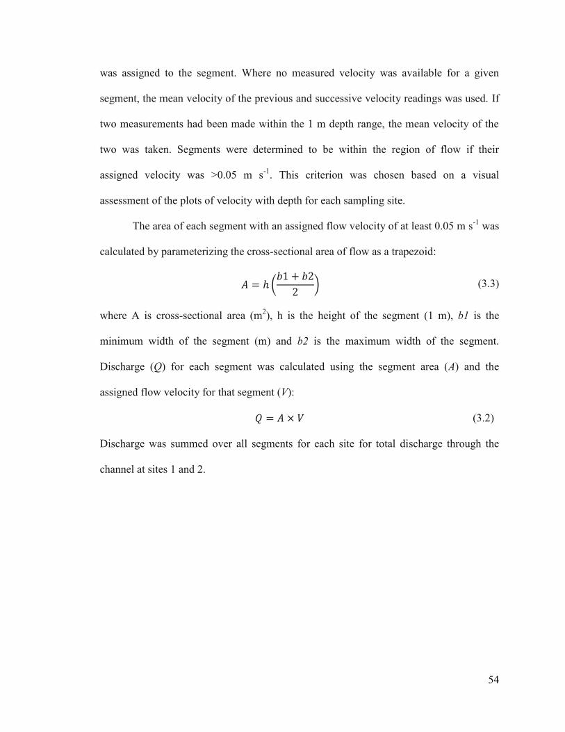
54

was assigned to the segment. Where no measured velocity was available for a given

segment, the mean velocity of the previous and successive velocity readings was used. If

two measurements had been made within the 1 m depth range, the mean velocity of the

two was taken. Segments were determined to be within the region of flow if their

assigned velocity was >0.05 m s-1

. This criterion was chosen based on a visual

assessment of the plots of velocity with depth for each sampling site.

The area of each segment with an assigned flow velocity of at least 0.05 m s-1

was

calculated by parameterizing the cross-sectional area of flow as a trapezoid:

𝐴 = ℎ (𝑏1 + 𝑏2

2) (3.3)

where A is cross-sectional area (m2), h is the height of the segment (1 m), b1 is the

minimum width of the segment (m) and b2 is the maximum width of the segment.

Discharge (Q) for each segment was calculated using the segment area (A) and the

assigned flow velocity for that segment (V):

𝑄 = 𝐴 × 𝑉 (3.2)

Discharge was summed over all segments for each site for total discharge through the

channel at sites 1 and 2.

55

4 Results

Ice thickness survey overview 4.1

Over the three field campaigns for this study, ~40 km of surface elevation and ice

thickness transects were completed, covering 5.5 km of the ~11 km long channel and 800

m of the ~7 km long fracture (Figures 4.1 and 4.2). Grid A had the lowest percentage of

traces for which the ice-water reflector was identified (63%, compared to >75% in other

grids) (Table 4.1). The ice shelf basal topography generally mirrored surface elevation as

the lowest elevation surface areas corresponded to areas with the thinnest ice. Thin ice is

seen along the length of the channel (grids A-D, Figure 4.2) and within the fracture (grid

E). Within the channel, ice was consistently thinnest in grid A (<5 m). The ridges and

troughs of the characteristic rolls on the ice shelf surface were also captured in the

thickness data presented here. This effect was most prominent in the vicinity of the

fracture, where survey lines across the fracture followed along these ridges and troughs:

lines of thin ice (troughs) can be seen alternating with thicker ice (ridges) extending on

either side of the fracture (box E, Figures 4.1 & 4.2).

Over the entire survey, the mean ice thickness was 41 m, with a minimum of 1 m

and maximum of 68 m. Ice thicknesses less than 3.4 m thick (25 MHz) and 1.7 m (50

MHz) are artefacts and represent errors in picking the correct location of the basal

reflector, because, as described previously, they exceed the minimum vertical resolution

possible with the respective antennae. The mean surface elevation was 4.37 m, and the

maximum was 8.89 m. The lowest surface elevation recorded was -0.86. Elevations

below sea level, however, are likely erroneous and attributed to a datum-related error; as

discussed in Chapter 5.

56

Figure 4.1 Map of point surface elevation measurements along IPR transect grids from a

Dual Frequency GNSS receiver unit post-corrected with Precise Point Positioning. Data

are overlaid on a July 2016 ASTER image of the Milne Ice Shelf. Grids are labelled by

letter on the map and inset boxes, black dashed lines indicate boundaries between grids.

57

Figure 4.2 Map of ice thicknesses measured along IPR transect grids. Data are overlaid

on a July 2016 ASTER image of the Milne Ice Shelf from July. Grids are labelled by letter

on map and inset boxes; black dashed lines indicate boundaries between grids.

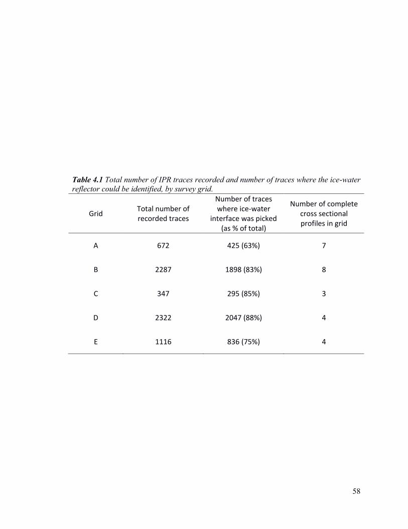
58

Table 4.1 Total number of IPR traces recorded and number of traces where the ice-water

reflector could be identified, by survey grid.

Grid Total number of recorded traces

Number of traces where ice-water

interface was picked (as % of total)

Number of complete cross sectional profiles in grid

A 672 425 (63%) 7

B 2287 1898 (83%) 8

C 347 295 (85%) 3

D 2322 2047 (88%) 4

E 1116 836 (75%) 4

59

Figure 4.3 shows a typical radargram from a cross-channel IPR transect. The continuous

black line seen at ~600 ns marks the ice surface. The strong, bright reflector arriving later

(~1400 ns on the left side of the profile) is the ice-ocean interface. The basal channel can

be seen cutting upward into the base of the ice shelf between traces 45 and 85,

interrupting the continuous basal reflector. Where the ice shelf is sloped along the walls

of the channel, accurately identifying the base of the ice is difficult due to noise from

multiple off-nadir returns and absent reflections, as seen in Figure 4.3. Therefore, there

are relatively few ice thickness measurements available from the sidewalls of the channel

in the cross-sectional profiles.

Channel morphology 4.2

In total, 22 complete channel cross-sections across the channel were identified (Table

4.1). There were four fracture cross-sections. These cross-sections were used to

characterize channel and fracture morphology (Table 4.2). For four of the cross-sections

from grid A, there were no picks made between the breakpoints defining the channel

banks, so channel height was only calculated using three of the seven cross sections.

The cross-sections from the channel all show a deeply-incised feature with

sloping sidewalls located beneath the E-W surface depression (Figure 4.4). Away from

the edge of the ice shelf, in grids B, C and D, basal width and incision height were fairly

consistent (Figure 4.4, Table 4.2). Mean channel widths ranged from 57 to 86 m and the

mean channel incision height across all three grids was 42 m, or 77% of the mean ice

shelf thickness of 55 m reported by Mortimer et al. (2012). Channel height decreased in

the down-channel direction. The channel was significantly broader and less deeply

incised at the seaward edge, in grid A, than it was at the grids up-channel

60

Figure 4.3 A radargram from a cross-channel profile in grid D. Multiple radar traces

are aligned side by side in a radargram, in order to show variation in the subsurface

over horizontal space. The continuous black line just below 600 ns is the ice surface. The

bright reflector at 1400 ns is the ice shelf-ocean interface. The channel can be seen in the

ice shelf from trace 45 to 90. On the sides of the channel, there are places where no

reflector can be seen or where identifying the correct reflector was not possible, due to

multiple reflections due to off-nadir reflections from the angled sidewall.

61

Table 4.2 Basal and surface morphology metrics calculated from all complete ice

penetrating radar cross-sectional profiles across the channel (grids A to D) and fracture

(grid E).

Grid

Mean width ±1 SD

(m)

Mean height ±1

SD (m) (as % of total )

Minimum ice

thickness (minimum

draft)

Mean ice thickness left bank

±1 SD (m)

Mean ice thickness

right bank ±1 SD (m)

Mean surface width ±1 SD (m)

Mean surface depth ±1 SD

(m)

Mean sidewall

slope angle ±1

SD (°)

A 164±12

n = 7 32±2 (58)

n = 3 3(3) 51±7 48±6

320±12 n = 7

6±1 n = 7

32±15

B 86±12 n = 8

39±3 (71) n = 8

6(6) 51±4 52±6 68±4 n = 5

3±1 n = 5

43±21

C 57±8 n = 3

43±2 (78) n = 3

10(9) 40.±2 59±2 NA NA 61±22

D 82±7 n = 4

45±4 (82) n = 4

10(5) 52±5 61±3 96±30 n = 2

3±1 n = 2

40±11

E 69±21 n = 4

43±4* (100) n = 4

4(3) – – – – 78±6

* for the fracture, mean depth was calculated, using the height of both sidewalls Metrics not calculated for the fracture are marked with – NA indicates metric could not be calculated Uncertainty associated with ice thickness measurements in this study is ±2.58 m

62

Figure 4.4 Two representative cross-sectional ice thickness profiles (one plotted in

green, one in black) from cross-channel (grids A to D) and cross-fracture (grid E)

transects. Channel profiles run from the left (negative) to right (positive) where the left is

defined in the downstream direction and zero corresponds to the centerline defined along

the channel at the surface of the ice shelf. Fracture profiles run from north (negative) to

south (positive) across the fracture; zero corresponds to the fracture centerline. Plots of

channel and fracture cross-sections not shown here are provided in Appendix A.

63

(χ2

width = 17.52, p<0.001; χ2

height = 14.99, p = 0.001). The minimum ice thickness at the

crest of the channel was in grid A (3 m) and thickness increased up channel to grid D (10

m) (Table 4.2). The maximum draft (ice <0 m asl) measured in the channel was 9 m, at

grid C.

The mean slope of the channel sidewalls, averaged across the left and right sides

of the channel, ranged from 32° at grid A to 61° at grid C (Table 4.2). The surface

depression was widest (320±12 m) and deepest (6±1 m) at grid A, and narrower and

shallower away from the ice shelf edge, consistent with the patterns noted in basal

morphology. There was considerable variability in surface morphology along the

channel. The depression was consistently narrow in grid B (68±4 m), but highly variable

in grid D (96±30 m). Notably, there was no appreciable depression at the surface of the

ice shelf overlying the channel in grid C.

A striking feature of the cross-sections was the asymmetrical nature of the profiles

from grid C and, to a lesser extent, grids B and D. Ice thicknesses on the left bank of the

channel were significantly less than ice thicknesses on the right bank in grids B (W =

2671.5, p = 0.009), C (W = 110, p<0.001) and D (W = 312, p<0.001) (Table 4.2). The

mean slope of the channel sidewalls in grid C also differed on the left and right sides. The

mean slope of the left channel wall at grid C was 42°, consistent with sidewall slope

angles at grids B and D but the right wall of the channel was much steeper, with a mean

slope of 80° (Figure 4.5). There were no significant differences in slope between the left

and right sidewalls of the channel in grid A (t = -0.49, p = 0.65), B (t = -0.67, p = 0.51) or

D (t = -0.44, p = 0.68) (Figure 4.5). While mean sidewall slope angles were fairly

consistent between grids, there was substantial variability in slope angle along each

64

Figure 4.5 Boxplots showing variability in mean sidewall slope angle up from horizontal,

calculated for each of the left and right sides of each cross-section, by grid. The right

side of the channel is substantially steeper at grid C, whereas there is no significant

difference in slope angle between the left and right sides for any other grid. The plot for

grid E shows that sidewall slope angles on both sides of the fracture are consistently

much steeper than those of the channel.

65

segment of the channel walls in individual cross sections, reflected in the standard

deviation (Table 4.2). Variability in the sidewall topography can also be seen in the

plotted cross-sections (Figure 4.4): there appear to be ‘steps’ incised into the channel

walls in the profiles from grid B near the base of the channel.

Comparison of fracture and channel morphology 4.3

The sidewalls of the fracture were substantially, and consistently, steeper than those of

the channel, with a mean slope angle of 78±6° (Table 4.2, Figure 4.5). Median ice

thickness in the fracture was 7 m (Figure 4.6), and ice thicknesses across the width of the

fracture were fairly consistent whereas channel ice thickness increased rapidly away from

the middle of the channel (Figure 4.4). The fracture was through the full ice shelf

thickness. The width of the fracture was quite variable in the cross sections surveyed

(Table 4.2). The cross-sections plotted in Figure 4.4 (grid E) illustrate an instance of a

transect along the crest of a ridge (higher surface elevation, black line) and a transect

along a trough between rolls (lower surface elevations, green line). The plotted cross-

section also show an instance where thin ice in a trough is not echoed at the base of the

ice shelf (green line) though Figure 4.1 and 4.2 show that generally, there was thin ice

along the troughs.

Additional ice thickness measurements 4.4

Ice thickness measurements made through natural cracks and steam-drilled boreholes in

the channel show ice thicknesses ~2 m in grid A, with thicker ice in grids B and C (Table

4.3). No additional ice thickness measurements were made in grid D. Ice thicknesses and

drafts measured through boreholes in grids B and C are comparable to those measured in

the channel with IPR (B: 5-6 m, C: ~8 m). Ice drafts of ~1 m measured around the

66

Figure 4.6 Boxplots showing variability in ice thicknesses measured with ice penetrating

radar within the channel (grids A, B, C and D) and within the fracture (E).

67

Table 4.3 Ice thickness and ice draft measurements made through natural cracks and

steam-drilled boreholes in the channel.

Grid Ice thicknesses (m)

A 1.75, 1.52, 1.65, 1.50,

1.68, 1.80, 1.81

B 3.27(draft), 3, 3.5,

7(draft)

C 8(draft)

D NA*

E 1.04, 1.50 (draft), 1.75

(draft), 1.33 (draft)

*NA indicates no ice thickness measurements were made through cracks or boreholes within the grid

68

profiling sites in the fracture are thinner than the minimum ice thicknesses that could be

measured with the IPR.

Characterization of snow cover 4.5

Snow depths were measured along several IPR transect lines in grid D. Snow depth

varied from 0.00 m to 2.60 m, with a median snow depth of 0.25 m (Figure 4.7). Peak

snow depth values were measured within the depression but snow depths within the

channel were also highly variable. Outside the depression, snow depths were more

consistent; depth was generally less than 0.5 m.

Hydrography 4.6

Temperature and salinity profiles 4.6.1

Temperature and salinity profiles from along-channel CTD transects in 2015 and 2016

show the structure of the near-surface water column within the channel, compared to that

of the epishelf lake and offshore of the ice shelf (Figure 4.8). The strongly stratified

epishelf lake has a layer of warm (>0°C) and fresh (SA <1 g kg-1

) water overlying colder,

more saline water (<1°C, SA > 25 g kg-1

) with a steep halocline and thermocline,

indicating the transition occurs over just a few meters. The depth of the epishelf lake was

10.3 m in July 2015 and 9.8 m in July 2016. The profile taken offshore shows seawater

through the entire depth of the profile, save for a very thin freshwater cap from seasonal

sea ice melt.

Profiles from within the channel are distinct from the epishelf lake and offshore

profiles. Channel profiles from both years and both sampling sites show a well-mixed

layer several meters thick present just below the ice at both channel sites. This layer had

temperatures (-1ºC to 0ºC) and salinities (5-14 g kg-1

) that were intermediate

69

Figure 4.7 Plots illustrating variability in snow depths measured along grid D IPR

transects. A boxplot of snow depths (A) shows that median snow depth was 0.25 m, with a

minimum of 0.00 and maximum of 2.60 m. A plot of snow depth (B) against distance from

the channel centerline shows that snow depths were most variable in the depression

overlying the channel; peak values were also located in the channel.

70

Figure 4.8 Temperature and salinity with depth for four locations in an along-channel

CTD transect done in 2015 and 2016. Only the upper water column, to 50 m depth, is

shown. Measurements taken within ice were removed from the top of the profiles and the

downcasts isolated. The solid black line indicates the profile taken offshore of the ice

shelf through a lead in the sea ice; the dashed line is the profile from sampling site 1 at

the seaward edge of the channel; the dotted line is the profile from sampling site 2

located roughly mid-channel and the solid grey line is the epishelf lake profile for each

year.

71

between the epishelf lake and offshore profiles. Below the brackish layer, salinity and

temperature gradually transition to that of ambient seawater by 30 m depth. At site 1 at

the seaward edge of the channel, however, the brackish layer was thinner, saltier and

cooler than the layer at site 2 in both years. Although there was some year to year

variability, the CTD profiles show that general salinity structure of the profiles, and the

spatial pattern seen along the CTD transect, were consistent over the two years of study.

Temperature and salinity profiles from the fracture in 2014, 2015, and 2016 are

plotted with epishelf lake and channel profiles in Figure 4.9. The structure of the water

column at the fracture site was not consistent year to year. In 2014, the fracture site and

epishelf lake profiles showed the same stratified structure with a freshwater layer to 9 m.

In 2015, only a thin freshwater layer was present and the water column was very weakly

stratified, indicative of mixing. In 2016, the fracture profile again had a distinct near-

surface freshwater layer, and had become more stratified than in 2015.

Current measurements 4.6.2

4.6.2.1 Channel

Plots of mean current speed with depth for sites 1 and 2 in the channel show a subsurface

jet of relatively fast flowing water from ~3-10 m depth (site 1) and from ~7-15 m depth

(site 2) (Figure 4.10). Above and below the jet, current speeds were substantially lower

(<5 cm s-1

). The highest current speed at site 1 (62±3 cm s-1

) was recorded at 5.4 m depth.

At site 2, the maximum current speed in the jet of 48±2 cm s-1

was recorded at 9.9 m

depth (Figure 4.10). The sampling increment was ~1.5 to 2 m at site 2, and even coarser

at site 1, so even faster water speeds may have occurred at un-sampled depths. Mean

current speed with depth at sites 1 and 2 is plotted against salinity in Figure

72

Figure 4.9 Salinity and temperature profiles for 2014, 2015 and 2016 showing profiles

from the fracture, plotted against profiles from the epishelf lake and the channel for the

same year for comparison. The channel was not profiled in 2014. For each profile,

measurements taken in ice were removed, and the downcast isolated. The epishelf lake

profile is shown with a solid line, the fracture with a dashed line and the channel profile

with a dotted line.

73

Figure 4.10 Mean water speed with depth at the seaward edge of the channel (site 1),

and approximately mid-way along the channel (site 2). Water speed was measured for 2

minutes at each depth, and the mean of the middle 80% of the recorded values taken.

Mean speed (in m s-1

) is plotted in red; points indicate the depths at which water speed

measurements were recorded. The dashed grey lines indicate one standard deviation

from the mean. Salinity with depth at each location is plotted in blue.

74

4.10. The region of fastest flow for both sites occurs within the halocline separating the

brackish layer and seawater.

Flow directionality in the channel was inferred from observations. When a

weighted line was lowered into the water column in the channel, the instrument line was

pulled sharply in the down-channel direction at depths consistent with the depth range of

the jet, causing the line to hang at an angle (Figure 4.11). This was observed in all

instances where current measurements were being made in the channel, at both sampling

sites. Therefore, flow in the channel was assumed to be primarily in the down-channel

(out-fiord) direction. No angling of the line was observed at any time when lowering

instruments into the water at the fracture.

4.6.2.2 Fracture

Current measurements in the fracture were collected with an ADCP so flow directionality

was recorded by the instrument. Flow velocities in the along-fracture (u axis) and along-

fiord directions (v axis) were uniformly low to 25 m, at least an order of magnitude

slower than flow recorded in the channel (Figure 4.12). Water velocities recorded along

the fracture (u axis) ranged from -0.9 to 0.7 cm s-1

, with a mean of -0.2±2.0 cm s1; there

was no dominant flow direction. Along the v axis, the range was – 1.2 to 2.3 cm s-1

, with

a mean of 0.8±2.2 cm s-1

. Flow occurred primarily in the positive v direction, which was

cross-fracture and roughly out of the fiord.

Estimation of discharge 4.6.3

Discharge calculated for each of the 1 m segments spanning the estimated thickness of

the outflow jet at sites 1 and 2 are shown in Table 4.4 and Table 4.5, respectively. Based

on these results, the total discharge through the channel at site 1 was 110.34 m3 s

-1 and

75

Figure 4.11 Photos of a weighted line lowered through a natural hole in the ice overlying

the channel. Panel A shows the line before the weight reached the depth of fast flowing

water: the line hung straight down into the water from the hand. Panel B shows the line

when it has been taken up by the fast flowing near-surface current. The line was pulled

downstream (left side of crack in the photo) and thus, angled away from vertical. The red

dashed line marks the vertical from the hand for comparison.

76

Figure 4.12 Time-averaged velocities with depth in the water column at the fracture. The

'u' axis is along the fracture, with positive u running NE, toward the intersection of the

fracture and channel. The 'v' axis is oriented roughly along-fiord, with positive v being

toward the ocean. Grey dashed lines indicated one standard deviation from the mean for

each depth. Depth bins are 1.5 m, with the center of the first bin at 2.33 m depth.

77

Table 4.4 Area, water velocity and discharge for each 1 m depth segment over the

estimated depth of flow in the channel at site 1. Discharge is summed across all segments

for total discharge.

Depth Range (m) Area (A, m

2) Velocity (V, m s

-1) Discharge (Q, m

3 s

-1)

3-4 41.81 0.37* 15.47

4-5 47.38 0.49 23.22

5-6 51.27 0.60* 30.76

6-7 55.16 0.40 22.06

7-8 59.26 0.20* 11.85

8-9 63.46 0.11 6.98

Total 110.34

*indicates a velocity reading was made with the current meter within the specified depth range

78

Table 4.5 Area, water velocity and discharge for each 1 m depth segment over the

estimated depth of flow in the channel at site 2. Discharge is summed across all segments

for total discharge.

Depth Range (m) Area (A, m

2) Velocity (V, m s

-1) Discharge (Q, m

3 s

-1)

7-8 17.10 0.13* 2.22

8-9 20.51 0.33* 6.77

9-10 21.42 0.46 9.86

10-11 23.43 0.45* 10.13

11-12 24.28 0.42 9.84

12-13 24.28 0.35* 8.50

13-14 25.33 0.23* 5.82

14-15 26.33 0.10* 2.63

Total 55.77

*indicates a velocity reading was made with the current meter within the specified depth range

79

55.77 m3 s

-1 at site 2. The vertical sampling resolution at site 1 was coarser than at site 2

(Figure 4.10, Tables 4.4 and 4.5) so it is less certain how representative interpolated

velocities are of actual flow in the jet. There were also no measurements of velocity made

at depths less than 3 metres at site 1, though it is suspected there would have been flow at

shallower depths given the relatively high flow velocity recorded between 3 and 4 m

(Table 4.4).

80

5 Discussion

Morphological evidence for channelization 5.1

Cross-sectional ice thickness profiles support the hypothesis that there is a channel

incised upward into the base of the Milne Ice Shelf. Cross-channel profiles along the E-

W surface depression show a deeply-incised, inverted ‘v’-shaped feature with sidewalls

that sloped upward on average ~40° from horizontal (Figure 4.4, Table 4.2). The

morphology of the purported channel is distinct from that of the fracture, which is

consistent with differing mechanisms of formation. The inverted ‘v’ shape of the channel

is consistent with upward thermal incision into the ice shelf by water, analogous to the

formation of a v-shaped valley by a river. The fracture, in contrast, rifted through the

entire thickness of the ice shelf as a result of tensile stresses which exceeded the strength

of the ice (Lawn, 1993). As a result, it had consistently near-vertical sidewalls (Table 4.2,

Figure 4.5). After formation, the fracture infilled with ice; ice thicknesses are therefore

uniformly thin across the fracture width rather than thickening toward the margins as in

the channel (Figure 4.6).

Observations of a channel with sloping sidewalls are consistent with the

morphology of basal channels detected beneath the floating tongue of the Petermann

Glacier in Greenland (Rignot and Steffen, 2008) and the Pine Island Glacier ice shelf in

Antarctica (Stanton et al., 2013). The surface morphology of the E-W depression is also

consistent with channelization. The presence of a surface depression overlying the

channel is consistent with downward deformation of ice toward hydrostatic equilibrium

as mass is removed from below (c.f. Vaughan et al., 2012). Longitudinal crevasses were

observed along the walls of the surface depression (Figure 1.3). The formation of

81

crevasses along the flanks of the surface depression overlying a basal channel have also

been noted on other ice shelves (Vaughan et al., 2012) and are attributed to bending

stresses induced as the ice shelf surface settles downward in response to gradually

reduced ice thickness above the channel (McGrath et al., 2012).

Controls on channel surface and basal morphology 5.2

The morphology of the surface depression overlying the channel was somewhat obscured

by snow deposition. Limited snow thickness measurements showed snow could be up to

several metres thick within the channel (Figure 4.7), so, in many locations, the depression

was likely deeper than indicated by the surface elevations presented herein. In addition,

snow deposition across the depression may also not have been homogenous across the

channel. The orientation of the channel with respect to the prevailing wind, or the effect

of local topographic surface variations, may have resulted in preferential accumulation in

certain aspects or locations over others.

Although the mean channel basal width was consistent between grids B and D,

the mean width of the surface depression in D (96±30 m) was wider and more variable

than that of grid B (68±4 m, Table 4.2). If the only factor determining surface depression

morphology was the downward deformation of the ice shelf surface to hydrostatic

equilibrium, it is expected that surface morphology would be reasonably consistent. At

grid C, there was no discernible surface depression overlying the channel at all.

Inconsistent infilling of the surface depression by snow may explain the variability in the

width of the surface depression between the survey grids. Variability may also be

attributed to variations in bridging stresses along the channel. The channel was narrowest

at grid C, and the ice thicknesses at the crest of the channel thickest, so it could be that

82

bridging stresses at that location were great enough that the surface of the ice shelf had

not yet slumped noticeably downward. An estimation of whether these surface elevation

measurements demonstrate that the ice is in hydrostatic equilibrium should be done. If the

ice shelf was not yet in hydrostatic equilibrium, further settling of the ice shelf surface

over the channel would be expected in future.

IPR survey grids were spaced along the length of the channel, with the aim of

investigating changes in channel morphology over distance. Channel basal morphology

(basal width, incision height and sidewall slope angle) was fairly consistent away from

the seaward edge of the ice shelf over the 5 km length spanned by grids B, C, and D

(Table 4.2). The channel appeared to be broader and less deeply incised at the edge of the

ice shelf in grid A, with a shallower mean sidewall slope angle as a result. However, the

differences in morphology noted at the edge of the ice shelf (grid A), are likely not

reflective of the channel proper.

Rather, the apparent widening is attributed to mistakenly surveying seaward of the

actual ice shelf edge. At the location of grid A, the ice shelf was notched inward and had

been infilled by MLSI (the Milne ‘re-entrant’ described by Jeffries, 1986). During the

IPR survey, many of the across-channel lines crossed from thick ice shelf ice onto the

thin sea ice, and back onto thick ice shelf ice on the other side of the notch, rather than

over ice shelf-ice thinned by incision. Therefore, no conclusion can be made about

whether channel morphology was significantly different at the seaward edge of the ice

shelf. It is expected that, had it been possible to survey the length of the channel, the

channel would be less incised with distance from the epishelf lake, as the potential for

melt (thermal driving) would lessen as heat was lost from epishelf lake outflow.

83

For four of the IPR transects across grid A, no reflections indicating the ice-water

interface could be identified in the thin ice between the thick channel banks. Grid A also

had the lowest percentage of traces in which the ice-water reflector could be identified

(Table 4.1). The lack of reflections across the channel in grid A is attributed to the

attenuation of the radar signal due to the presence of the conductive saline MLSI, coupled

with ice thicknesses in the channel that were thinner than the minimum resolvable by the

IPR antenna frequency used. Ice thicknesses measured through cracks and steam-drilled

boreholes were 1.50 to 1.75 m in the middle of the channel in grid A (Table 4.3). A 50

MHz antenna was used to survey grid A, for which the minimum detectable thickness

was calculated to be 1.7 m in Section 3.3.2. Where ice is too thin, the air and reflected

waves overlap so it was not possible to identify and pick the location of the ice shelf base

in many locations.

Previous studies of basal channel morphology have identified both smooth-sided

basal channels (Rignot and Steffen, 2008; Stanton et al., 2013) and channels with

terraced sidewalls (Dutrieux et al. 2014). Dutrieux et al. (2014) described terraced

channel geometry in two different settings, on both an Antarctic ice shelf (Pine Island

Glacier) and the Petermann Glacier (Greenland), leading them to conclude terraced

melting could be a generic feature of melting in an ice shelf channel. Topographic

variability along a channel results from heterogeneous melt patterns; they suggest that it

is specifically uneven melt due to stratification in the ice-ocean boundary layer within a

channel that leads to terracing. Variability in slope angles calculated along the channel

walls in this study show there is local (metre-scale) topographic variability along the

84

channel walls (Table 4.2), and cross sectional profiles are suggestive of the existence of

stepped topography near the base of the channel for grids B and D (Figure 4.4).

Although terracing noted by Dutrieux et al. (2014) is on scale much larger than

what was observed here (terraces hundreds of metres wide in Antarctica and Greenland),

it is plausible that the steps seen here are also caused by stratified flow and heterogeneous

melt rates. Indeed, the CTD profiles from within the channel collected in this study,

discussed in section 5.3, suggest flow is stratified within the channel beneath Milne Ice

Shelf (Figure 4.8). The steps identifiable in the cross-sectional profiles occur 30 to 50 m

below the top of the channel. At this depth, the CTD profiles from the channel indicate

there is no influence from the epishelf lake as water properties are consistent with

ambient ocean water (Figure 4.8). The formation of steps would presumably occur near

the top of the channel where the warm epishelf lake outflow is in contact with the channel

sides. These steps are unlikely to be the result of active incision, but they may be ‘legacy’

channel features, formed earlier when the channel was less deeply incised.

If steps are formed sequentially as the channel is incised, steps may be expected

along the height of the channel walls, which is not seen in these data. However, the full

extent of topographic variations along the channel walls is not well resolved by the

methods used here, since a detailed geometry of the channel walls is hampered by the

presence of noise from multiple reflectors off the steeply angled walls (e.g. Figure 4.3).

The channel, therefore, may appear artificially smooth away from the channel base, due

to the linear interpolation used to fill in missing thicknesses. Some of the apparent

variability in sidewall slope angle is undoubtedly the result of errors in the determination

of the correct position of the basal reflector, but erroneous picks are unlikely to account

85

for all the observed variability. Conversely, the presence of terraced topography also

controls melt rates (Dutrieux et al., 2014), so an understanding of detailed channel

morphology may be an important element in understanding melt and channel evolution.

Minimum ice thicknesses at the crest of the channel measured in the IPR survey

were 6±2.58 m in grid B, and 10±2.58 m in both grids C and D. Ice thicknesses are

consistent with those made through cracks and boreholes in grids B and C (Table 4.3) and

with findings by Mortimer (2011) of ice <10 m thick in the channel based on a limited

number of cross-sections in 2008-2009. Mortimer et al. (2012) also identified a large area

of thin ice (~20-30 m) abutting the southern side of the channel near the confluence of the

channel and the N-S fracture formed prior to 1950 (Figure 1.4). They measured much

greater ice thicknesses on the opposing side of the channel (upwards of 50 m). The

presence of this anomalous area of thin ice, combined with depth soundings that showed

the sea bed rose to within 28 m of the surface led Hamilton (2016) to conclude the ice

shelf was likely grounded on a seabed ridge that rises beneath the ice shelf and extends 2

km south of the fracture. Findings of differential reflectivity from the ice shelf base in

this area by Narod et al. (1988) are also consistent with a grounded ice shelf.

The area of thin ice detected by Mortimer et al. (2012) and the location of the

depth sounding by Hamilton (2016) are coincident with the location of the asymmetrical

ice thickness profiles from grid C, where thicknesses were significantly less on the left

(south) side of the channel (40±2 m) than on the right (north) side (59±2 m). This effect

is also seen in profiles from grids B and D, though it is less pronounced (Table 4.2,

Figure 4.4). The results presented here provide corroborating evidence for a locally

grounded ice shelf. Further, the ice thickness profiles may help to constrain the extent of

86

the seabed ridge, as they show that the ice shelf might be grounded for as much as 4 – 5

km (the distance between grids B, C, and D) along the south bank of the channel. Future

work should examine the nature of basal reflectivity on either side of the channel, as an

additional line of evidence for a grounded ice shelf.

Differing slope angles on the left and right sides of the channel in profiles from

grid C might be the result of variability in melt rates due to an asymmetrical flow velocity

profile in the channel at grid C. Deflection of flow to the right wall of the channel and the

associate elevated velocities could have accelerated melting along the right wall, for

instance, similar to the development of a steep cut bank on the outside of a river meander.

Modelling investigations of channel formation have shown that the deflection of flow

through a channel by the Coriolis force could result in preferentially higher melt rates to

one side and, thus, asymmetry in channel side slope angle (Millgate et al., 2013).

However, the scale of the channel on the Milne Ice Shelf is much smaller than the

range of the Rossby radius of deformation for the Arctic (e.g. Cottier et al., 2010) so

deflection by the Coriolis force does not explain why the right side of the channel is

steeper at grid C. Local deflection of flow due to curvature in the channel is a possible

explanation; RADARSAT-2 imagery and photos of the surface depression (Figure 1.3)

do show some meandering along the channel. Perhaps differential hydrostatic adjustment

of grounded and ungrounded ice due to mass removal (or gain, if accretion occurred at

the ice shelf base for some reason) also had an impact on side slope asymmetry. It is

possible that side slope asymmetry is somehow related to the left-right asymmetry in ice

thicknesses at grid C since, for instance, if the ice shelf is grounded in this location,

perhaps a local deflection of flow occurs as a result of the influence of sea bed

87

topography there. The difference in side slope angle could also be related to differential

movement of the ice shelf on the right and left sides of the ice channel as a result of

grounding. If ice on the right side of the channel is moving relative to the other one side

of the channel (because only the floating side is adjusting to hydrostatic equilibrium as

the ice shelf thins), then perhaps the ongoing deformation of the ice along the channel can

explain the observed morphology.

The data suggest that channelized melt produced the observed surface and basal

morphology, but ice shelf grounding is a plausible mechanism to explain the initiation of

this channelized flow beneath the Milne Ice Shelf. If the ice shelf was indeed locally

grounded, tensile stresses (from differential movement of the grounded and ungrounded

ice in response to tides, for example) may have resulted in weaknesses/fractures within

the ice, or basal crevassing, along the grounded/ungrounded boundary. Over many years,

outflow from the epishelf lake could then have been preferentially directed along this

weakness, resulting in upward incision and the observed channel morphology. This

potential model for channel formation is consistent with Keys’ (1978) assertion that

channelization would be unlikely to be initiated by epishelf lake outflow alone, as any

incipient channel would fill with frazil ice as the thin outflow layer cooled. A large

volume of outflow directed through an existing weakness, in contrast, would have a high

heat content and thus, high melt potential.

Properties of flow through the channel 5.3

Current measurements, coupled with CTD profiles of the channel water column, confirm

that the channel was a drainage pathway for the epishelf lake. A fast-flowing jet of water

flowing in the down-channel direction was detected at both sampling locations in the

88

channel. Peak flow velocities recorded at both sites in the channel (40-60 cm s-1

, Figure

4.10) are an order of magnitude higher than velocities measured below the halocline of

the epishelf lake (i.e. where outflow could theoretically occur) (1-2 cm s-1

, Hamilton,

2016) or velocities measured along either axis at the fracture (Figure 4.12, 1-2 cm s-1

).

Tidal dynamics cannot explain flow velocities of the observed magnitude, as the tidal

range in the fiord is very small (Hamilton, 2016). The presence of the jet therefore

suggests that outflow is being concentrated in the channel. The observation of the fast

flowing jet at both sampling sites in the channel, coupled with the consistent surface and

basal morphology along the channel, also confirms the channel is continuous and

connected.

The thickest ice along the outflow channel acts as a constriction and so, controls

flow through the channel and the depth of the epishelf lake. It seems likely the

constriction is located in the area of grid C. Minimum ice drafts measured at the crest of

the channel in grid C with IPR and through a steam drilled borehole were 8-9 m whereas

drafts on either side along the channel in grids B and D were much less (Tables 4.2, 4.3).

Though there is uncertainty associated with ice thickness measurements, a draft of ~9 m

is roughly consistent with the measured depth of the epishelf lake in July 2015 (10. 3 m)

and July 2016 (9.8 m) since it is expected that the freshwater layer would be distinctly

deeper than the minimum draft by July, at the height of the melt season, due to inflow.

The exact properties of the warm outflowing epishelf lake water depend on the depth of

the outflow layer. At 9 m depth in 2015 and 2016, water in the epishelf lake had a

temperature of ~1°C and an absolute salinity of <1 g kg-1

, whereas by 10 m depth, water

had an absolute salinity of ~15 g kg-1

but was still ~1°C in temperature (Figure 4.8).

89

It can be seen from the velocity profiles from site 2 that outflow did not occur right at the

top of the channel but rather, peak velocities occurred within the halocline at 9.9 m depth

(Figure 4.10). The water flowing out of the epishelf lake in the jet is fresher and more

buoyant than the seawater beneath the ice shelf, but denser than the fresh water being

generated at the top of the channel through submarine melting of the ice shelf (and from

the injection of surface meltwater in some cases). As a result, the outflow jet is vertically

constrained by density stratification, and it cannot rise up against the base of the ice shelf.

Sampling resolution is poor at site 1 but flow appears to be shallower and closer to the ice

shelf base; velocity at 5.4 m depth was 62±3 cm s-1

. This may be because stratification of

the water column lessens downstream (e.g. because less melt is generated as the heat

content of the jet diminishes), allowing the jet to rise higher up in the channel.

The outflow jet transported the warm and comparatively fresh epishelf lake water

through the channel, which modified the structure of the water column. If there was no

epishelf lake outflow in the channel, a water column structure resembling a typical

offshore profile would be expected, with a very thin layer of surface meltwater

transitioning quickly to seawater. Instead, at the depth of the jet, water in the channel is

warmer and fresher than seawater, consistent with outflow. However, with distance from

the epishelf lake, the halocline shoals upward, and water in the jet is cooler and saltier,

indicating the water column was becoming more and more well-mixed with distance

along the channel. Therefore, it is concluded that the velocity of the jet must be sufficient

to overcome stratification in the channel and cause turbulent mixing, at least in some

places along the channel.

90

Both sites 1 and 2 had a connection between the ice shelf surface and the channel, as

sampling was done through natural cracks in the ice, and surface meltwater was observed

to flow into these cracks. The addition of surface meltwater may have altered the

structure of the water column somewhat at the sites sampled (e.g. the thickness of the

meltwater layer at the top of the channel impacts at what depth the outflow jet can flow).

Nonetheless, the hydrographic profiles here clearly demonstrate epishelf lake water was

flowing through the channel and the similarity in flow velocities measured at channel

sites separated in space suggests velocity measurements were fairly representative.

The morphology of the channel and the presence of epishelf lake water in the

channel are consistent with the idea that warm epishelf lake outflow transports heat into

the channel causing localized melting and channelization. As previously described, the

outflow jet was vertically constrained due to stratification in the channel, so it flowed a

few metres below the top of the channel. The presence of a mixed layer at the top of the

channel overlying the warmer epishelf lake water may mean that there is insufficient heat

at the top of the channel for significant melt, so melting may be concentrated along the

sides of the channel where velocities are highest. There may even be freezing occurring

at the top of the channel while melting occurs along the sides, as has been theorized to

occur in some basal crevasses (Khazendar and Jenkins, 2003). With distance from the

epishelf lake, water in the jet was cooler and more saline, as heat was presumably lost to

melting and as more cold seawater was mixed upward (Figure 4.8). Therefore, melt rates

in the channel are expected to decrease with distance from the epishelf lake. Indeed,

channel incision heights calculated here decreased slightly in the down-channel direction

(from grids D to B) which is consistent with decreasing melt rates.

91

Freshwater input to the epishelf lake occurs from early-June to mid-August during the

melt season, resulting in a corresponding deepening of the epishelf lake (Hamilton,

2016). When inflow ceases, the epishelf lake gradually thins as excess freshwater flows

out of the channel. Outflow beneath the ice shelf is non-linear and drainage occurs at a

rate proportional to the difference between the minimum ice draft and the epishelf lake

depth (Hamilton, 2016). Therefore, discharge through the channel increases over the melt

season, reaching a maximum at the end of the melt season in mid-August when the

epishelf lake is deepest. Heat content of the epishelf lake also increases over the melt

season (Hamilton, 2016). Consequently, outflow velocities and the structure of the water

column (temperature, salinity and thickness of the mixed layer), as well as the resulting

melt patterns, are presumed to vary over the course of the year. Melting may be ongoing,

or may have seasonal modulation. Future work should focus on obtaining hydrographic

measurements over time, to understand how the velocity, thickness, flow depth and

temperature of the outflow jet changes over the year, as these dynamics will impact melt

and channel evolution.

Discharge 5.4

Discharge through the channel was estimated at 110 m3 s

-1 at site 1 in the channel, and 56

m3 s

-1 at site 2 (Tables 4.4 and 4.5). The estimate from site 2 is likely more reliable than

that from site 1, due to a higher density of velocity measurements through the depth of

flow there. In addition, the location of site 1 in grid A may also mean that this discharge

measurement is not representative of flow through the channel because this location may

not be within the channel proper, as previously discussed. Nonetheless, while there is

uncertainty in these estimates, discharge calculated for site 2 in particular is likely a

92

reasonable first order approximation of the magnitude of epishelf lake outflow volume

directed through the channel for the date sampled.

To explore how important the channel might be in draining the epishelf lake, an

estimate of total outflow from the epishelf lake is required for comparison. The available

estimates for outflow are bulk annual estimates. Using the glacier mass budget for the

northern Canadian Arctic Archipelago for 2000 – 2011 estimated by Lenaerts et al.

(2013), the total meltwater runoff from the 1108 km2 Milne Fiord catchment is estimated

to be at least 1.12×109

m3 a

-1 by Hamilton et al. (2017). The percentage of this runoff that

enters the fiord at the surface and contributes to the epishelf lake is likely between 10 and

28%, based on observed changes in the depth of the epishelf lake (Hamilton et al., 2017).

Assuming that 30% of the total meltwater runoff enters the epishelf lake as inflow, and

that over the course of the year all inflow leaves the epishelf lake as outflow, this gives a

total outflow estimate of 3.4×108 m

3 a

-1.

Discharge in this study was measured on a day in mid-July, which is approximately

midway through the melt season (mid-June to mid-August). The lake deepens over the

melt season, reaching a maximum depth in mid-August, and outflow from the epishelf

lake increases with the depth of the freshwater layer (Hamilton et al., 2017). Therefore,

the outflow volume through the channel in mid-July is unlikely to represent the

maximum discharge volume reached over the melt season. Outflow from the epishelf

lake occurs during the entire year, but it would be much lower in early June when the

epishelf lake is at its lowest. If, as a rough estimate, the discharge value from site 2 is

taken to be something close to mean discharge volume over the two month melt season,

then the total outflow volume through the channel over 2 months is ~2.9×108 m

3. On this

93

approximation, outflow through the channel during the summer alone would account for

85% of the total annual outflow of 3.4×108 m

3 as calculated above. If the discharge from

site 1 were used, the estimate of outflow through the channel would be even higher.

While these estimates for discharge through the channel and total outflow from the

epishelf lake are highly simplified, and it is beyond the scope of this thesis to do a

detailed accounting of inflow and outflow, discharge data are a first look at the relative

importance of the channel in draining the epishelf lake. These calculations suggest that

outflow through the channel is at least the same order of magnitude as total outflow from

the epishelf lake and, further, that it is possible the channel is indeed an important

drainage pathway for the epishelf lake.

This interpretation is supported by the findings of Hamilton et al. (2017), who

showed that observed changes in the depth of the Milne Fiord epishelf lake were well

modelled assuming that outflow was directed through a constriction of similar

dimensions to the one mapped herein. Additionally, findings by previous investigators

suggested that the only ice thin enough to constitute an outflow channel beneath the ice

shelf is along the E-W feature (Narod et al., 1988; Hamilton et al., 2017, Figure 1.4).

There are no other candidate surface depressions or fractures on the ice shelf that could

represent outflow conduits (Figure 1.3A). Therefore, it seems plausible that the channel

documented here accounts for the majority of the water leaving the Milne Fiord epishelf

lake.

Fracture hydrography and morphology 5.5

The fracture had similar water properties to the epishelf lake, which suggests there was

connectivity between the fracture and the main body of the epishelf lake. Epishelf lake

94

water in fractures within the ice shelf have been previously noted, indicating a network of

fractures must connect the main body of the epishelf lake to these ‘satellite’ lakes

(Hamilton, 2016). There was, however, variability in the depth of the freshwater layer in

the fracture between the years surveyed. In 2014, the depth of the freshwater layer was

identical to that of the main epishelf lake (Figure 4.9). ADCP measurements showed

negligible flow along and across the channel in 2014, consistent with the presence of

strong stratification of the water column that year (Figure 4.12).

In 2015, however, the water column structure in the fracture did not resemble that

of the main epishelf lake. The gradient of the halocline and thermocline were much

gentler and the stratified structure was disturbed (Figure 4.9). The freshwater layer

thinned to just a few meters. In 2016, though, it appeared the epishelf lake may have been

once again developing within the fracture, as the freshwater layer had deepened and the

halocline steepened. However, while was evidence from the CTD profiles that mixing

had occurred, no appreciable flow was noted in the fracture in either 2015 or 2016 when

a weighted instrument line was lowered into the water column, as noted earlier.

The seeming recovery of the stratified structure of the water column in 2016,

coupled with the fact that there was no flow through the fracture, indicates that the

disruptions of the stratified water column structure in the fracture were the result of

temporary events and not, say, the result of outflow through the fracture. Mixing at the

fracture may have been caused by an isolated (and time-limited) mixing event that caused

localized changes to the water column structure in the fracture. This phenomenon is not

unknown in Milne Fiord; a sudden decrease in the thickness of the main epishelf lake in

January 2012 was attributed to an episodic mixing event by Hamilton (2016). Internal

95

waves, tidal oscillations and iceberg calving events outside the fiord have all been

suggested as possible mechanisms which could generate energy for episodic mixing

(Veillette et al., 2008; Hamilton et al., 2017). Alternatively, the connection between the

fracture could be ephemeral and the 2015/2016 profiles were taken while the fracture was

draining and/or refilling of the fracture with epishelf lake.

The presence of the epishelf lake water in the 2009 fracture helps to further

constrain the specific location of the ice shelf dam, i.e. the constriction that controls the

depth of the epishelf lake and marks the beginning of channelized outflow. The fracture

intersects the channel very close to the fiordward end of the channel. The dam must be

seaward of the fracture or the epishelf lake would not have been present there, as it would

have drained out through the channel. Combined with the ice draft measurements along

the channel, this further suggests the constriction is in the area of grid C.

Ice thickness measurements showed that along most of the troughs between rolls in

the vicinity of the fracture, ice was very thin (<10 m), but along one, ice thicknesses in

the troughs were comparable to those beneath roll crests (Figures 4.1 & 4.2, Figure 4.4).

Though these findings represent a fairly small sample area, they shed some light on the

ongoing question of whether (or to what degree) the rolling surface topography on the

surface of the ice shelf is echoed at the base (Jeffries, 2017). These results seem to

suggest the base is not a mirror image of the surface, but that significant topographic

variability at the ice shelf base is related to surface topography. Narod et al. (1988), in

contrast, found that there was little to no bottom expression of the surface rolls on the

Milne Ice Shelf. However, the IPR survey lines along the rolls and troughs only extend to

96

~200 m on either side of the fracture, so it cannot be said how widespread this pattern is

from these data.

If the thinning is localized, it may be the result of lateral melting along the fracture

walls by the warm epishelf lake water in the fracture. The concentration of melt along

certain troughs is still perhaps suggestive of some dampened initial variability in ice

thickness on the underside of the ice shelf resulting in preferential melt along the thinner

ice, however. White et al. (2015) also noted thin ice in troughs on the Petersen Ice Shelf,

and ice islands from the Petersen Ice Shelf appeared to be ridges that had broken away

from the ice shelf along troughs. The findings of White et al. (2015) imply that the results

presented here, of thin ice in troughs, could be very significant in terms of ice shelf

stability as they represent zones of weakness that could make the Milne Ice Shelf more

prone to fracture.

Sources of error 5.6

Minimum absolute surface elevations measured in this study were below 0 m asl (Figure

4.1), but the ice surface was not observed to be depressed below sea level at any location.

Negative surface elevations are attributed to the vertical datum used as a reference for

surface elevations. The datum used in this study to post-process locational data was the

CGVD28 datum. The accuracy of heights derived with CGVD28 in southern Canada is

±5 cm, whereas in northern regions the accuracy is on the order of decimeters because

there are few accurate and known CGVD28 height benchmarks that can be used for

correction in northern Canada (Hughes Clark et al., 2005). Uncertainty in absolute

surface elevation does not present a problem in interpreting the results in this study,

97

because relative elevations and ice thicknesses are not affected assuming the error in

vertical position is constant over the small area surveyed.

There was also uncertainty in ice thickness measurements due to picking errors

which was quantified using a cross-point analysis (Table 3.2). While the median

difference in cross-points was 1.4 m, there were some instances with very large

disagreement between cross-points. Error in ice thicknesses reported here is attributed

primarily to differences in the apparent depth of the bed reflection between down-channel

and across-channel IPR transects where basal topography was steeply sloped. A pulse of

energy transmitted by a radar system is not focused, but spreads out as it travels through

the ice (Hubbard and Glasser, 2005). Therefore, where the ice is sloped, reflected energy

is returned from points upslope of the point directly below the midpoint of the transmitter

and receiver (the nadir), as well as from the nadir (the location of the desired reflector).

Steep basal topography, such as the side slopes of the channel in this study, result in

multiple off-nadir reflections (Bauder et al., 2003), which makes it difficult to determine

the true location of basal reflections in survey lines that travel longitudinally along or

adjacent to a steep slope.

Along-channel IPR transects were highly susceptible to multiple reflections from

the channel sidewalls because profiles were along the slope, while cross-channel transects

were less affected. Large errors in ice thickness were most likely the result of a correct

pick of the bed reflection in the cross-channel line and an erroneous pick in the along-

channel line. However, while the cross-point analysis used points from the intersection of

along- and across-channel transects, only cross-channel profiles were used to generate

98

plots of ice thickness with distance across the channel/fracture and calculate geometry.

Therefore, large errors in picks are unlikely to plague cross-channel profiles.

The presence of meltwater ponds and wet slush in the depression also prevented

picks from being made in many cases, as the radar signal was attenuated by water and

there was no bed reflection. In some cases, ice thicknesses were recorded that are thinner

than the minimum resolvable thickness for the antennae used (the minimum ice thickness

reported in Chapter 4 was 1 m). Nonetheless, although there were errors in the selection

of the correct reflector particularly where ice was thin, ice thicknesses measured along

the channel banks and within the channel are in good agreement with previous studies

(Mortimer, 2011; Mortimer et al., 2012). Additionally, ice thicknesses measured through

steam-drilled boreholes and natural cracks within the channel compare very well with

coincident IPR results (Tables 4.2 & 4.3), providing confidence in this analysis.

Implications of channelization for ice shelf stability 5.7

Thin ice overlying the basal melt channel represents a significant structural weakness in

the Milne Ice Shelf. Reduced mechanical strength along the channel means the ice shelf

is likely to be particularly vulnerable to fracturing along this weakness. Crevassing along

the channel at the surface of the ice shelf is also an indicator of reduced ice shelf stability

due to channelization (Vaughan et al., 2012). Ice thicknesses at the crest of the channel

are already as little as 6 m in some locations. As described previously, the 2001-2002

breakup of the Ward Hunt Ice Shelf is thought to have occurred along a basal channel

incised by epishelf lake outflow, where ice thickness were ~25 m, compared to mean

thicknesses of 40-60 m (Mueller et al., 2003). The drainage of the epishelf lake dammed

by the Petersen Ice Shelf may have initiated in a similar way. A ‘meandering fissure’ was

99

noted running from the epishelf lake along the margin of the ice shelf and the location of

this fissure coincided with the thinnest ice surveyed on the ice shelf (White et al., 2015).

Increased incision of the Milne Ice Shelf is expected in a warming climate.

Meltwater runoff is predicted to more than double over this century (Lenaerts et al.,

2013). Increased inflow into the epishelf lake will cause increased outflow through the

channel. Increased outflow volume will result in augmented heat transport to the channel,

leading to higher melt and incision rates in the channel. Repeat ice thickness

measurements at one location in the channel showed that overlying ice thickness had

already decreased from ~40 m in 1981 to <10 m in 2008/2009 (Mortimer, 2011). Based

on the change in the depth of the epishelf lake, Hamilton (2016) estimated that the

minimum draft of the ice shelf (the ice dam) thinned a further 5.4 m between 2009 and

2014. If the ice shelf does not fracture along the channel first, enhanced melt along the

channel as a result increased outflow could incise completely through the ice overlying

the channel in the next 5 to 10 years.

100

6 Conclusion

The aim of this study was to determine whether epishelf lake outflow was channelized

beneath the Milne Ice Shelf. The results of this study support the hypothesis that a

curvilinear depression that ran E-W across the outer region of the ice shelf was the

surface expression of a basal channel and confirm that outflow occurred along this

channel.

The first objective of this study was to characterize the morphology of the

suspected channel and compare it to a straight stress fracture that formed on the ice shelf

in 2009. Ice penetrating radar was used to map ice thicknesses in several survey grids

along the length of the ~11 km channel. Cross-sectional ice thickness profiles revealed an

inverted ‘v’-shaped basal channel with sloping sidewalls beneath the surface depression,

consistent with incision of the ice shelf by warm water. The mean slope of the channel

sidewalls ranged from ~40 to 60°. Ice thickness data from grid A were determined not to

be representative of the channel but rather the result of surveying seaward of the ice shelf

edge. Away from the edge, in grids B, C and D, the channel was 57- 86 m wide at the

base and was incised 39-40 m upward into the ice shelf, which was >70% of the mean ice

shelf thickness. Ice thicknesses at the crest of the channel were as little as 6±2.58 m. The

fracture, in contrast, had rifted through the entire ~40 m thickness of the ice shelf. It had

steeply sloping parallel sidewalls and was infilled with uniformly thin ice (<5 m).

The surface morphology of the channel was also consistent with channelization.

The presence of a depression is consistent with channelization, formed as unsupported ice

deforms downward to hydrostatic equilibrium. Stresses induced as the ice surface settles

results in the formation of crevasses along the flanks of the channel at the surface;

101

longitudinal crevassing was observed at several locations along the length of the channel.

Variability in the width of the depression along the length of the fracture might result

from infilling by snow, and/or along-channel differences in bridging stresses that

determines the ice shelf response to the removal of mass from below.

Channel morphology at grid C was notably different than it was within 1-2 km on

either side in grids B or D. The cross-sections from grid C showed that ice thicknesses

were significantly less on the left side of the channel than on the right side. The right side

of the channel was also much more steeply sloped than the left side (80° compared to

42°). Asymmetry in ice thickness was seen in profiles from B and D, but was much less

pronounced; mean sidewall slope angles were consistent for both sides of the channel in

grids B and D. Previous investigators have suggested the Milne Ice Shelf was locally

grounded on a sea bed ridge in the vicinity of the channel. Asymmetrical cross-channel

profiles presented here seem to be consistent with grounding along the inner edge of the

channel, but further work needs to be done to confirm grounding.

The second objective of this study was to profile the temperature and salinity of

the water in the channel, as well as current speed and direction, to determine whether

they were consistent with epishelf lake outflow. Conductivity-temperature-depth (CTD)

profiling of the water column in the channel, coupled with the current measurements,

confirmed warm, brackish outflow from the epishelf lake flowed through the channel.

Flow velocities >60 cm s-1

were recorded in the channel, which was an order of

magnitude higher than flow recorded in the epishelf lake or in the fracture, indicating that

outflow was concentrated in the channel. Peak velocities of the outflow jet occurred

within the halocline, several metres below the top of the channel due to the stratification

102

of the channel water column. Stratified flow may also mean melt in the channel is

concentrated along the channel sides, rather than the top. The stratified nature of flow in

the channel may also have influenced the development of local variations (steps) in the

channel sidewalls.

The final objective of the study was to calculate discharge through the channel.

Discharge at site 1 was estimated at 110.34 m3

s-1

, and 55.77 m3 s

-1 at site 2. While it

cannot be concluded from these data alone that the channel is the primary drainage

pathway for the Milne Fiord epishelf lake, when compared with inflow estimates, the

discharge volumes calculated for the channel in this study seem consistent with findings

of previous investigators who suggest that the channel was the primary conduit for

outflow from the epishelf lake. Based on hydrographic profiling of the 2009 fracture and

minimum ice drafts along the channel, it was determined the ice shelf dam, or

constriction point that controls outflow from the epishelf lake, was most likely located a

few km seaward of the confluence of the fracture and channel. Outflow occurred along

the entire length of the channel, exiting at the seaward edge of the ice shelf. These results

contribute to an understanding of the dynamics of Milne Fiord and the processes

operating at the base of the ice shelf.

This study provides the first confirmation of a basal channel under an ice shelf in

the Canadian Arctic. The presence of a basal channel beneath an ice shelf decreases its

stability. Thin ice along the length of the channel represents an area of weakness that

makes the Milne Ice Shelf increasingly vulnerable to stresses. Channelization of epishelf

lake outflow may have been an important factor in deglaciation along the northern coast

of Ellesmere Island: observations suggest previous ice shelf breakup events in the

103

Canadian Arctic occurred along areas of thin ice formed by channelization. The Milne Ice

Shelf may also be vulnerable to break up along thin ice in troughs between the ice shelf

rolls, though more work is required to elucidate the extent and cause of thin ice in the

troughs. Future breakup of the Milne Ice Shelf is likely to occur along the channel in the

near future, resulting in the drainage of the last epishelf lake in the Northern Hemisphere.

Building on these results, the next step should be modelling the rate of incision of

the ice shelf by epishelf lake outflow, in order to understand channel evolution. Detailed

channel morphology, current speed and water temperature and salinity data from this

study make it possible to model basal melt rates along the channel and estimate the

incision rate of the ice shelf by epishelf lake outflow. Mass loss and runoff are projected

to increase in the Canadian Arctic Archipelago in a warming climate (Gardner et al.,

2011; Lenaerts et al., 2013). An increase in runoff input into the Milne Fiord epishelf

lake will result in increased outflow and consequently, increased incision rates and a

further reduction in ice thickness. An understanding of melt rates is therefore necessary to

understand channel evolution and ice shelf stability in a warming climate.

There exist few direct measurements of water properties or current speed in ice

shelf basal channels, due to the difficulty of accessing ice shelf cavities (e.g. Rignot and

Steffen, 2008; Stanton et al., 2013). Though the exact values are specific to the channel

beneath the Milne Ice Shelf, in-situ observations from this study will contribute to an

improved understanding of how the presence of basal channels can alter ice-shelf ocean

interactions. Understanding controls on ice shelf stability is important because the

collapse of ice shelves along the coasts of Greenland and Antarctica will result into

greater flux of ice into the ocean from the continent, contributing to global sea-level rise.

104

Quantitative data from this study can be used to develop and validate models of ice ocean

processes and, thus, better predictions about ice shelf stability and change in a warming

climate.

105

7 References

Alley, K.E., Scambos, T.A., Siegfreid, M.R., and Fricker, H.A. (2016) Impacts of warm

water on Antarctic ice shelf stability through basal channel formation. Nature

Geoscience, 9: 290-293.

Annan, A.P. (2009) Electromagnetic Principles of Ground Penetrating Radar. In Jol, H.

ed. Ground Penetrating Radar Theory and Applications, Elsevier, Oxford,

England.

Antoniades, D., Francus, P., Pienitz, R., St-Onge, G., and Vincent, W.F. (2011) Holocene

dynamics of the Arctic’s largest ice shelf. Proceedings of the National Academy

of Sciences. 108(47): 18899-18904.

Arcone, S., Lawson, D., and Delaney, A. (1995) Short-pulse radar wavelet recovery and

resolution of dielectric contrasts within englacial and basal ice of Matanuska

Glacier, Alaska, U.S.A. Journal of Glaciology, 41(137): 68-86.

Bauder, A., Funk, M., and Gudmundsson, G.H. (2003) The ice-thickness distribution of

Unteraargletscher, Switzerland. Annals of Glaciology, 37: 331-336.

Braun, C. Hardy, D.R., and Bradley, R.S. (2004) Surface mass balance of the Ward Hunt

Ice Rise and Ward Hunt Ice Shelf, Ellesmere Island, Nunavut, Canada. Journal of

Geophysical Research, 109(D22110).

Cassidy, N.J. (2009) Ground penetrating radar data processing, modelling and analysis.

In Jol, H. ed. Ground Penetrating Radar Theory and Applications, Elsevier,

Oxford, England.

106

Clark, T.S. and Bentley, C.R. (1994) High resolution radar on Ice Stream B2, Antarctica:

measurements of electromagnetic wave speed in firn and strain history from

buried crevasses. Annals of Glaciology, 20: 153-59.

Copland, L., Mueller, D.R., and Weir, L. (2007) Rapid loss of the Ayles Ice Shelf,

Ellesmere Island, Canada. Geophysical Research Letters, 34(L21501).

Copland, L., Mortimer, C., White, A., Richer McCallum, M., and Mueller, D. (2017)

Factors contributing to recent Arctic ice shelf losses. In Copland, L., and Mueller,

D.R. eds. Arctic Ice Shelves and Ice Islands, Springer, Dordrecht, The

Netherlands, in press.

Cottier, F.R., Nilsen, F., Skogseth, R., Tverberg, V., Skardhamar, J. and Svendsen, H.

(2010) Arctic fjords: a review of the oceanographic environment and dominant

physical processes. In Howe, J.A., Austin, W.E.N., Forwick, M and Paetzel, M.

eds. Fjord Systems and Archives, Special Publication, Geological Society,

London, 344: 35-50.

Crary, A.P. (1960) Arctic ice island and ice shelf studies, Part II. Arctic, 13: 32-50.

Dowdeswell, J.A. (2017) Eurasian Arctic ice shelves and tidewater ice margins. In

Copland, L., and Mueller, D.R. eds. Arctic Ice Shelves and Ice Islands, Springer,

Dordrecht, The Netherlands, in press.

Drewry, D.J., Jordan, S.R., and Jankowski, E.J. (1982) Measured properties of the

Antarctic Ice Sheet: surface configuration, ice thickness, volume, and bedrock

characteristics. Annals of Glaciology, 3: 83-91.

107

Dutrieux, P., Vaughan, D.G., Corr, H.F.J., Jenkins, A., Holland, P.R., Joughan, I., and

Fleming, A.H. (2013) Pine Island Glacier ice shelf melt distributed at kilometer

scales. The Cryosphere, 7(5): 1543-1555.

Dutrieux, P., Stewart, C., Jenkins, A., Nicholls, K.A., Corr, H.J., Rignot, E.R. and

Steffen, K. (2014) Basal terraces on melting ice shelves. Geophysical Research

Letters, 41: 5506-5513.

England, J.H., Lakeman, T.R., Lemmen, D.S., Bednarksi, J.M., Stewart, T.G., and Evans,

D.J.A. (2008) A millennial-scale record of Arctic Ocean sea ice variability and

the demise of the Ellesmere Island ice shelves. Geophysical Research Letters,

35(L19502).

Fisher, E., McMechan, G.A., and Annan, A.P. (1992) Acquisition and processing of

wide-aperture ground-penetrating radar data. Geophysics, 57(3): 495-504.

Gardner, A.S., Moholdt, G., Wouters, B., Wolken, G.J., Burgess, D.O., Sharp, M.J.,

Cogley, J.G., Braun, C., and Labine, C. (2011) Sharply increased mass loss from

glaciers and ice caps in the Canadian Arctic Archipelago. Nature, 473(7347):

357-360.

Gibson, J., and Andersen, D. (2002) Physical structure of epishelf lakes of the southern

Bunger Hills, East Antarctica. Antarctic Science, 14(3): 253-261.

Gladish, C.V., Holland, D.M., Holland, P.R. and Price, S.F. (2012) Ice-shelf basal

channels in a coupled ice/ocean model. Journal of Glaciology, 58(212): 1227-

1244.

Hamilton, A.K. (2016) Ice-Ocean Interactions in Milne Fiord. PhD thesis, University of

British Columbia, Vancouver, Canada. 151 pp.

108

Hamilton, A.K., Laval, B.E., Mueller, D.R., Vincent, W.F. and Copland, L. (2017)

Dynamic response of an Arctic epishelf lake to seasonal and long-term forcing:

implications for ice shelf thickness. The Cryosphere Discussion, doi:10.5194/tc-

2017-19.

Hattersley-Smith, G. (1963) The Ward Hunt Ice Shelf: recent changes of the ice front.

Journal of Glaciology, 4: 415-424.

Holdsworth, G. (1971) Calving from Ward Hunt Ice Shelf, 1961-1962. Canadian Journal

of Earth Sciences, 8(2): 299-305.

Holdsworth, G., and Glynn, J. (1981) Iceberg calving from floating glaciers by a

vibration mechanism. Nature, 274: 464-466.

Holland, P.R., Jenkins, A., and Holland, D.M. (2008) The Response of ice shelf basal

melting to variations in ocean temperature. Journal of Climate, 21: 2558-2572.

Hubbard, B. and Glasser, N. (2005) Field Techniques in Glaciology and Glacier

Geomorphology. John Wiley & Sons Ltd, West Sussex, England.

Hughes Clarke, J.E., Dare, P., Beaudoin, J., and Bartlett, J. (2005) A stable vertical

reference for bathymetric surveying and tidal analysis in the high Arctic. U.S.

Hydrographic Conference, San Diego, California, USA. 16 pp.

Humbert, A., Steinhage, D., Helm, V., Hoerz, S., Berendt, J., Leipprand, E., Christmann,

J., Plate, C., and Muller, R. (2015) On the link between surface and basal

structures of the Jelbart Ice Shelf, Antarctica. Journal of Glaciology, 61(229):

975-986.

Jeffries, M. O. (1986) Glaciers and the morphology and structure of the Milne Ice Shelf,

Ellesmere Island, N.W.T., Canada. Arctic and Alpine Research, 18(4): 397-405.

109

Jeffries, M.O. (1991) Perennial water stratification and the role of basal freshwater flow

in the mass balance of the Ward Hunt Ice Shelf, Canadian High Arctic. In Weller,

G., Wilson, C.L. and Severin, B.A.B. eds. Proceedings of the International

Conference on the Role of Polar Regions in Global Change Vol 1, Fairbanks,

Alaska, USA: 332-337.

Jeffries, M.O. (1992) Arctic ice shelves and ice islands: origin, growth and disintegration,

physical characteristics, structural-stratigraphic variability and dynamics. Reviews

of Geophysics, 30(3): 245-267.

Jeffries, M.O. (2002) Ellesmere Island ice shelves and ice islands. In Williams, R.S. Jr

and Ferrigno, J.G. eds. Satellite Image Atlas of Glaciers of the World: Glaciers of

North America, U.S: Geological Survey Professional Paper 1386-J-1, Reston, VA,

USA: 147-163.

Jeffries, M.O. (2017) The Ellesmere ice shelves, Nunavut, Canada. In Copland, L., and

Mueller, D.R. eds. Arctic Ice Shelves and Ice Islands, Springer, Dordrecht, The

Netherlands, in press.

Jeffries, M.O., and Sackinger, W.M. (1988) Water circulation and ice accretion beneath

Ward Hunt Ice Shelf (Northern Ellesmere Island, Canada), deduced from salinity

and isotope analysis of ice cores. Annals of Glaciology, 10: 68-72.

Jenkins, A. (1991) A one-dimensional model of ice shelf-ocean interaction. Journal of

Geophysical Research: Oceans, 96(C11): 20671-20677.

Jenkins, A. (2011) Convection-driven melting near the grounding lines of ice shelves and

tidewater glaciers. Journal of Physical Oceanography, 41(12): 2279-2294.

Jungblut, A.D., Mueller, D.R., and Vincent, W.F. (2017) Arctic ice shelf ecosystems. In

110

Copland, L., and Mueller, D.R. eds. Arctic Ice Shelves and Ice Islands, Springer,

Dordrecht, The Netherlands, in press.

Kelley, D. and Richards, C. (2016) oce: Analysis of Oceanographic Data. R package

version 0.9-2.0. http://CRAN.R-project.org/package=oce.

Keys, J.E., Johannssen, O., and Long, A. (1968) On the oceanography of Disraeli Fiord

on Northern Ellesmere Island. Marine Sciences Centre Manuscript Report 6,

McGill University, Montreal, Canada.

Keys, J.E. (1978) Water regime of Disraeli Fiord, Ellesmere Island. Technical Report

792, Defence Research Establishment, Ottawa, Canada.

Khazendar, A., and Jenkins, A. (2003) A model of marine ice formation within Antarctic

ice shelf rifts. Journal of Geophysical Research, 108(C7): 3525.

Langley, K., von Deschwanden, A., Kohler, J., Sinisalo, A., Matsuoka, K., Hattermann,

T., Humbert, A., Nost, O.A., and Isaksson. E. (2014) Complex network of

channels beneath an Antarctic ice shelf. Geophysical Research Letters, 41(4):

1209-1215.

Lawn, R. (1993) Fracture of Brittle Solids, 2nd

ed. Cambridge University Press,

Cambridge, England.

Lazzara, M., Jezek, K., Scambo, T., MacAyeal, D., and Van der Veen, C. (1999) On the

recent calving of icebergs from the Ross Ice Shelf. Polar Geography, 23: 201-

212.

Le Brocq, A., Ross, N., Griggs, J.A., Bingham, R.G., Corr, H.J., Ferraccioli, F., Jenkins,

A., Jordan, T.A., Payne, A.J., Rippin, D.M. and Siegert, M.J. (2013) Evidence

111

from ice shelves for channelized meltwater flow beneath the Antarctic Ice Sheet.

Nature Geoscience, 6: 945-948.

Lemmen, D.S., Evans, D.J. & England, J. (1988) Ice shelves of northern Ellesmere

Island, NWT. The Canadian Geographer, 32: 363-367.

Lenaerts, J., Angelen, J.H., Broeke, M.R., Gardner, A.S., Wouters, B., and Meijgaard, E.

(2013) Irreversible mass loss of Canadian Arctic Archipelago glaciers.

Geophysical Research Letters, 40(5): 870-874.

Mankoff, K.D., Jacobs, S.S., Tulaczyk, S.M., and Stammerjohn, S.E. (2012) The role of

Pine Island Glacier ice shelf basal channels in deep-water upwelling, polynyas

and ocean circulation in Pine Island Bay, Antarctica. Annals of Glaciology,

53(60): 123-128.

McDougall, T.J. and Barker, P.M. (2011) Getting Started With TEOS-10 and the Gibbs

Seawater (GSW) Oceanographic Toolbox, SCOR/IAPSO WG127, ISBN 978-0-

646-55621-5. 28 pp.

McGrath, D., Steffen, K., Rajaram, H., Scambos, T., Abdalati, W., and Rignot, E. (2012)

Basal crevasses on the Larsen C Ice Shelf, Antarctica: Implications for meltwater

ponding and hydrofracture. Geophysical Research Letters, 39(L16504).

Millgate, T., Holland, P.R., Jenkins, A., and Johnson, H.L. (2013) The effect of basal

channels on oceanic ice-shelf melting. Journal of Geophysical Research: Oceans,

118: 6951-6964.

Mingo, L., and Flowers, G.E. (2010) Instruments and methods: An integrated lightweight

ice-penetrating radar system. Journal of Glaciology, 56(198): 709-714.

112

Mortimer, C.A. (2011) Quantification of Changes for the Milne Ice Shelf, Nunavut,

Canada, 1950-2009. MSc. thesis, University of Ottawa, Ottawa, Canada. 185 pp.

Mortimer, C.A., Copland, L., and Mueller, D.R. (2012) Volume and area changes of the

Milne Ice Shelf, Ellesmere Island, Nunavut, Canada, since 1950. Journal of

Geophysical Research, 117(F04011).

Mueller, D.R., Vincent, D.F., and Jeffries, M.O. (2003) Break-up of the largest Arctic ice

shelf and associated loss of an epishelf lake. Geophysical Research Letters,

30(20): 1-4.

Mueller, D.R., Vincent, W.F., and Jeffries, M.O. (2006) Environmental gradients,

fragmented habitats and microbiota of a northern ice shelf cryoecosystem,

Ellesmere Island, Canada. Arctic, Antarctic and Alpine Research, 38(4): 593-607.

Mueller, D.R., Copland, L., Hamilton, A., and Stern, D. (2008) Ice shelf break-up and

ecosystem loss in the Canadian High Arctic. EOS, 84(49): 548-552.

Mueller, D.R., Crawford, A., Copland, L., and Van Wychen, W. (2013) Report to the

Northern Transportation Assessment Initiative, Innovation Policy Branch,

Transport Canada, Ottawa, Canada.

Mueller, D.R., Copland, L., and Jeffries, M. (2017a) Changes in Canadian Arctic ice

shelf extent since 1906. In Copland, L., and Mueller, D.R. eds. Arctic Ice Shelves

and Ice Islands, Springer, Dordrecht, The Netherlands, in press.

Mueller, D.R., Copland, L. and Jeffries, M.O. (2017b) Northern Ellesmere Island ice

shelf and ice tongue extents, v 1.0 (1906-2015). Nordicana D28.

113

Narod, B.B., Clarke, G.K.C., and Prager, B.T. (1988) Airborne UHF sounding of glaciers

and ice shelves, northern Ellesmere Island, Arctic Canada. Canadian Journal of

Earth Sciences, 25(1): 95-105.

Navarro, F., and Eisen, O. (2010) Ground penetrating radar. In Pelikka, P and Rees, W.

eds. Remote Sensing of Glaciers: Techniques for Topographic, Spatial and

Thematic Mapping of Glaciers, CRC press/Balkema, Leiden, The Netherlands.

Overland, J., Key, J., Hanna, E., Hanssen-Bauer, B-M., Kim, S-J., Walsh, J., Wang, M.,

Bhatt, U., Liu, Y., Stone, R., Cox, C., and Walden, V. (2014) The Arctic. The

lower atmosphere: air temperature, clouds and surface radiation. In: “State of the

Climate 2014”. Bulletin of the American Meteorological Society, 95(7): S115-

S117.

Plewes, L.A. and Hubbard, B. (2001) A review of the use of radio-echo sounding in

glaciology. Progress in Physical Geography, 25(2): 203-236.

RD Instruments (2011) Acoustic Doppler Current Profiler Principles of Operation: A

Practical Primer. Teledyne RD Instruments Inc., Poway, California, USA.

Richer McCallum, M. (2015) Analysis of Ice Types Along the Northern Coast of

Ellesmere Island, Nunvavut, Canada and Their Relationship to Synthetic Aperture

Radar (SAR) Backscatter. MSc. thesis, Carleton University, Ottawa, Canada. 147

pp.

Rignot, E., and Steffen, K. (2008) Channelized bottom melting and stability of floating

ice shelves. Geophysical Research Letters, 35(L02503).

Scambos, T., Hulbe, C., and Fahnestock, M. (2003) Climate-induced ice shelf

disintegration in the Antarctic Peninsula. Antarctic Research Series, 79: 79-92.

114

Sergienko, O.V. (2013) Basal channels on ice shelves. Journal of Geophysical Research:

Earth Surface, 118: 1342-1355.

Stanton, T.P., Shaw, W.J., Truffer, M., Corr, H.F.J., Peters, L.E., Riverman, K.L.,

Bindschadler, R., Holland, D.M., and Anandakrishnan, S. (2013) Channelized ice

melting in the ocean boundary layer beneath Pine Island Glacier, Antarctica.

Science, 341: 1236-1239.

Stroeve, J.C., Serreze, M.C., Holland, M.M., Kay, J.E., Malanik, J., and Barrett. A.

(2012) The Arctic’s rapidly shrinking sea ice cover: a research synthesis. Climatic

Change, 110: 1105-1027.

Vaughan, D.G., Corr, H.F.J., Bindschadler, R.A., Dutrieux, P., Gundmundsson, G.H.,

Jenkins, A., Newman, T., Vornberger, P., and Wingham. D.J. (2012) Subglacial

melt channels and fracture in the floating part of Pine Island Glacier, Antarctica.

Journal of Geophysical Research: Earth Surface, 117(F03012).

Veillette, J., Mueller, D.R., Antoniades, D., and Vincent, W.F. (2008) Arctic epishelf

lakes as sentinel ecosystems: Past, present and future. Journal of Geophysical

Research: Biogeosciences, 113(G04014).

Veillette, J., Lovejoy, C., Potvin, M., Harding, T., Jungblut, A.D., Antoniades, D.,

Chenard, C., Suttle, C.A., and Vincent, W.F. (2011) Milne Fiord epishelf lake: a

coastal Arctic ecosystem vulnerable to climate change. Ecoscience, 18(3): 304-

316.

Vincent, W.F., Gibson, J.A.E., Pienitz, R., and Villeneuve, V. (2000) Ice shelf microbial

ecosystems in the High Arctic and implications for life on snowball Earth.

Naturwissenschaften, 87: 137-141.

115

Vincent, W. F., Gibson, J.A.E., and Jeffries, M.O. (2001) Ice shelf collapse, climate

change, and habitat loss in the Canadian high Arctic. Polar Record, 37(201): 133–

142.

Vincent, W.F., Whyte, L.G., Lovejoy, C., Greer, C.W., Laurion, I., Suttle, C.A., Corbeil,

J., and Mueller, D.R. (2009) Arctic microbial ecosystems and impacts of extreme

warming during the International Polar Year. Polar Science, 3(3): 171-180.

Vincent, W.F., Fortier, D., Levesque, E., Boulanger-Lapointe, N., Tremblay, B., Sarrazin,

D., Antoniades, D., and Mueller, D.R. (2011) Extreme ecosystems and

geosystems in the Canadian High Arctic: Ward Hunt Island and vicinity.

Ecoscience, 18(3): 236-261.

Welch, B.C., Pfeffer, W.T., Harper, J.T., and Humphrey, N.F. (1998) Mapping subglacial

surface of temperate valley glaciers by two-pass migration of a radio-echo

sounding survey. Journal of Glaciology, 44(146): 164-170.

White, A., Copland, L., Mueller, D., and Van Wychen, W. (2015). Assessment of

historical changes (1959-2012) and the causes of recent break-ups of the Petersen

Ice Shelf, Nunavut, Canada. Annals of Glaciology, 56(69): 65-76.

Wilson, N. (2013) Radar Tools (software). http://doi.org/10.5281/zenodo.43972

116

Appendix A: Cross-sectional ice thickness profiles from IPR survey

grids

Figure A1 Cross-sectional ice thickness profiles from grid A in the channel, used in the

calculation of metrics in Table 4.2 but not shown in Figure 4.4. Channel profiles run

from the left (negative) to right (positive) where the left is defined in the downstream

direction and zero corresponds to the centerline defined along the channel at the surface

of the ice shelf. The dashed grey line indicates sea level (0 m asl).

117

Figure A2 Cross-sectional ice thickness profiles from grid B in the channel, used in the

calculation of metrics in Table 4.2 but not shown in Figure 4.4. Channel profiles run

from the left (negative) to right (positive) where the left is defined in the downstream

direction and zero corresponds to the centerline defined along the channel at the surface

of the ice shelf. The dashed grey line indicates sea level (0 m asl).

118

Figure A3 Cross-sectional ice thickness profile from grid C in the channel, used in the

calculation of metrics in Table 4.2 but not shown in Figure 4.4. Channel profiles run

from the left (negative) to right (positive) where the left is defined in the downstream

direction and zero corresponds to the centerline defined along the channel at the surface

of the ice shelf. The dashed grey line indicates sea level (0 m asl).

119

Figure A4 Cross-sectional ice thickness profiles from grid D in the channel, used in the

calculation of metrics in Table 4.2 but not shown in Figure 4.4. Channel profiles run

from the left (negative) to right (positive) where the left is defined in the downstream

direction and zero corresponds to the centerline defined along the channel at the surface

of the ice shelf. The dashed grey line indicates sea level (0 m asl).

120

Figure A5 Cross-sectional ice thickness profiles from grid E (the fracture) used in the

calculation of metrics in Table 4.2 but not shown in Figure 4.4. Fracture profiles run

from north (negative) to south (positive) across the fracture; zero corresponds to the

fracture centerline. The dashed grey line indicates sea level (0 m asl).