CHANGING CORRELATIONS IN NETWORKS: ASSORTATIVITY …

Vol. 36 (2005) ACTA PHYSICA POLONICA B No 5

CHANGING CORRELATIONS IN NETWORKS:

ASSORTATIVITY AND DISSORTATIVITY∗

R. Xulvi-Brunet and I.M. Sokolov

Institut für Physik, Humboldt Universität zu Berlin

Newtonstraße 15, 12489 Berlin, Germany

(Received January 5, 2005)

Dedicated to Professor Andrzej Fuliński on the occasion of his 70th birthday

To analyze the role of correlations in networks, in particular, assorta-tivity and dissortativity, we introduce two algorithms which respectivelyproduce assortative and dissortative mixing to a desired degree. In bothprocedures this degree is governed by a single parameter p. Varying this pa-rameter, one can change correlations in networks without modifying theirdegree distribution to produce new versions ranging from fully random(p = 0) to totally assortative or dissortative (p = 1), depending on thealgorithm used. We discuss the properties of networks emerging when ap-plying our algorithms to a Barabási–Albert scale-free construction. In spiteof having exactly the same degree distribution, different correlated networksexhibit different geometrical and transport properties. Thus, the averagepath length and clustering coefficient, as well as the shell structure andpercolation properties change significantly when modifying correlations.

PACS numbers: 05.50.+q, 89.75.Hc

1. Introduction

Our interest to complex networks was strongly motivated by our studiesof models of infection spread, since it got clear that many effects can onlybe described when taking into account that an infecting agent spreads notin a homogeneous population of infectives, but over a complex network ofcontacts [1–3]. In many cases the exact knowledge of the network structureis necessary, in other situations one can rely on simple model assumptions,which, however, mirror the properties of a real networked system.

∗ Presented at the XVII Marian Smoluchowski Symposium on Statistical Physics,

Zakopane, Poland, September 4–9, 2004.

(1431)

1432 R. Xulvi-Brunet, I.M. Sokolov

Examples of systems described as complex networks are abundant inmany disciplines of science and have received much attention in the last fewyears. Thus, technological systems such as the World Wide Web, Internet,and electrical power grids, as well as other natural and social systems likechemical reactions in the living cell, different social collaboration networks,etc., have been successfully described through scale-free networks, networkswith power-law degree distributions P (k) ∼ k−γ [4, 5]. The degree distri-bution P (k) is one of the principal measures used to capture the structureof a network and represents the probability that a node chosen at randomis connected with exactly k other vertices of the network. The network ofhuman sexual contacts also has a property of being scale-free [6].

It was recently pointed out that real networks exhibit a degree of correla-tions among their nodes [7–20]. Thus, in social networks nodes having manyconnections tend to be connected with other highly connected nodes [8,10].This characteristic is usually referred to as assortativity, or assortative mix-ing. On the other hand, technological and biological networks show theproperty that nodes having high degrees are preferably connected with nodeshaving low degrees, a property referred to as dissortativity [7, 11].

Correlations play an important role in the characterization of the topol-ogy of networks, and therefore, they are essential to understand spreading ofinformation or infections, as well as their robustness against targeted or ran-dom removal of their elements [21–26]; in the case of infection such removalcorresponds to immunization of a part of the population. In order to deter-mine the exact influence of correlations several authors have proposed pro-cedures to build correlated networks [7,28–30]. The most general proceduresare the ones proposed by Newman [7] and Boguñá and Pastor-Satorras [30],who suggested two different ways to construct general correlated networkswith predeterminate correlations. Following the same goal, we, however,adopt a different perspective. Instead of putting in correlations “by hand”we propose to use link-restructuring (“rewiring”) processes [31] satisfyingconditions such as “nodes with similar degree connect preferably” (assorta-tive mixing) or “nodes with low degree try to connect with highly connectednodes” (dissortativity), leaving all other properties random.

Such processes, which do not change the degree distribution of networksand do avoid the appearance of multiple and self-connections, can be viewedas ergodic Markovian chains defined on the set of the network’s configura-tions. Repeated application of a rewiring step leads to distributions of linkconfigurations which converge to a stationary distribution with desired cor-relation properties, independently of the initial correlations of the network.In this work we thus introduce two procedures to change correlations basedon the rewiring of links, which produce assortative and dissortative mixing,respectively. Both algorithms are governed by a single parameter, p, and

Changing Correlations in Networks: Assortativity and . . . 1433

are capable to change the degree of assortativity (dissortativity) to a desiredamount allowing us to generate networks ranging from fully uncorrelated tototally assortative (dissortative). In the present work we focus on undirectednetworks. Some of the results were earlier reported on in Refs. [29, 33].

2. The assortative model

2.1. Algorithm

Starting from a given network, two links of the network connecting fourdifferent nodes are randomly chosen at each step. We consider the four nodesassociated with these two links, and order them with respect to their degrees.Then, with probability p, the links are rewired in such a way that one linkconnects the two nodes with the smaller degrees and the other connects thetwo nodes with the larger degrees; otherwise the links are randomly rewired(Maslov–Sneppen algorithm [16]). In the case that one or both of these newlinks already existed in the network, the step is discarded and a new pair ofedges is selected. This restriction prevents the appearance of multiple edgesconnecting the same pair of nodes. A repeated application of the rewiringstep leads to an assortative version of the original network. Note that thealgorithm does not change the degree of the nodes involved and thus theoverall degree distribution in the network. Changing the parameter p, it ispossible to construct networks with different degrees of assortativity.

2.2. Correlations and assortativity

Let Eij be the probability that a randomly selected edge of the networkconnects two nodes, one with degree i and another with degree j. Theprobabilities Eij determine the correlations of the network. We say thata network is uncorrelated when

Eij = Erij = (2 − δij)

iP (i)

〈i〉

jP (j)

〈j〉, (1)

i.e., when the probability that a link is connected to a node with a certaindegree is independent from the degree of the attached node. Here 〈i〉 = 〈j〉denotes the first moment of the degree distribution, assumed to be finite.

Assortativity means nodes with similar degrees tend to be connectedwith a larger probability than in the uncorrelated case, i.e., Eii > Er

ii ∀i.The degree of assortativity of a network can thus be characterized by thequantity [7]

A =

∑

i Eii −∑

i Erii

1 −∑

i Erii

, (2)


which takes the value 0 when the network is uncorrelated and the value 1when the network is totally assortative. (Note that in a finite network theconstraint that no pair of vertices is connected by more than one edge boundsA from above by the values lower than 1 [27].)

Now, starting from the algorithm generator, we can obtain a theoreticalexpression for Eij as a function of p. Let Eij be the number of links in thenetwork connecting two nodes, one with degree i and another with degree j,so that Eij = Eij/L, where L is the total number of links of the network.(Since undirected networks satisfy Eij = Eji, the restriction i ≤ j can beimposed without loss of generality.) We now define the variable

Fln =

n∑

r=l

n∑

s=r

Ers , r ≤ s , l ≤ n . (3)

Every time the rewiring procedure is applied, the values of Fln either in-crease or decrease by unity, or do not change. We can then calculate theprobabilities of change, i.e., that Fln → Fln +1 or Fln → Fln − 1. The effectof multiple edges can be disregarded since they are rare in the thermody-namical limit. Taking all corresponding possibilities into account, we obtainthe following expressions for the probabilities of change:

(Xln − fln)2 + p (Xln − f1n + f1,l−1)2 , for Fln → Fln + 1 ,

fln [(1−p)(1−2Xln) + p (X1,l−1−f1,l−1−f1n) + fln] , for Fln → Fln−1 .

Here fln = Fln/L, and Xln is given by

Xln =1

〈k〉

n∑

k=l

kP (k) , l ≤ n .

Using these expressions, we can calculate the expected value of fln. The pro-cess of repeatedly applying our algorithm corresponds to an ergodic Markovchain, and the stationary solution is given by the condition

(Xln − fln)2 + p (Xln − f1n + f1,l−1)2

= fln

[

(1 − p)(1 − 2Xln) + p(X1,l−1 − f1,l−1 − f1n) + fln

]

, (4)

for all l > 1. For l = 1 this condition reduces to

(1 + p) (X1n − f1n)2 = (1 − p)f1n [1 − 2X1n + f1n] . (5)


Using Eq. (4) and Eq. (5) we calculate fln. The solution reads

fln =X2

ln + (Bn − Bn−1)2

(1 − p)/2 + pXln + Bn + Bn−1

, l ≤ n ,

with

Bn =

√

[

pX1n +1 − p

4

]2

− pX21n

(

1 + p

2

)

.

Applying the definition, Eq. (3), we obtain the correlations

Eij = fij − fi,j−1 − fi+1,j + fi+1,j−1 . (6)

We note that Eq. (6) reduces to the corresponding uncorrelated case Erij

when p = 0, and reduces to

Eij = δij

iP (i)

〈i〉, (7)

for the case p = 1.

2.3. Properties of an assortative network

Let us start this section with drawing a small network to show howour algorithm works. The initial network is a Barabási–Albert scale-freeconstruction [32] with only N = 200 nodes and L = 400 links, see Fig. 1(a).To obtain other networks with exactly the same degree distribution butdifferent degree of assortativity we apply the algorithm discussed. Fig. 1shows the changes in the network with varying parameter p. In the figurewe have placed the nodes in such a way that nodes of degree 2 are shown inthe left part of each panel, all nodes of degree 3 lie to the right of any nodeof degree 2, all nodes of degree 4 lie to the right of any node of degree 3, etc.The nodes of the same degree are randomly spread within the correspondingarea of the figure to better show the links.

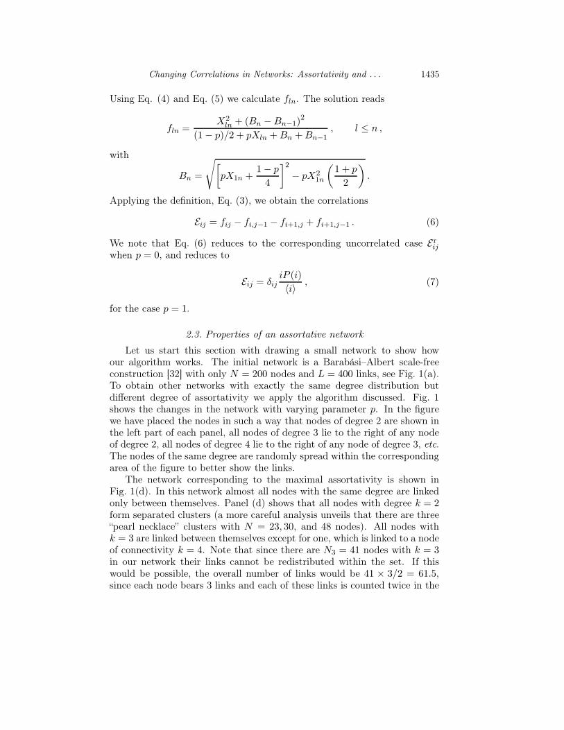
The network corresponding to the maximal assortativity is shown inFig. 1(d). In this network almost all nodes with the same degree are linkedonly between themselves. Panel (d) shows that all nodes with degree k = 2form separated clusters (a more careful analysis unveils that there are three“pearl necklace” clusters with N = 23, 30, and 48 nodes). All nodes withk = 3 are linked between themselves except for one, which is linked to a nodeof connectivity k = 4. Note that since there are N3 = 41 nodes with k = 3in our network their links cannot be redistributed within the set. If thiswould be possible, the overall number of links would be 41 × 3/2 = 61.5,since each node bears 3 links and each of these links is counted twice in the


(a)

A = 0

(b)

A = 0.26

(c)

A = 0.43

(d)

A = 0.62

Fig. 1. Scale-free networks for different degrees of assortativity (see text for details).

The nodes of the same degree are grouped together; the degree is nondecreasing

from left to right. The panels show: (a) A = 0 (uncorrelated network), (b) A =

0.26, (c) A = 0.43, (d) A = 0.62 (maximal assortativity).


set. All nodes with degree k = 4 form a single cluster, with two outgoinglinks, one to the cluster of nodes with k = 3, and one to a cluster of nodesof connectivity k = 5. In fact, the network is not a set of isolated clustersof nodes with the same connectivity only due to the restrictions imposed bythe given degree distribution. These restrictions are also responsible for thefact that A < 1 (for our network the maximal assortativity is Amax = 0.62).

In the present work we apply the algorithm to the Barabási–Albert con-struction with the number of links being twice the number of nodes L = 2N ,just like in our example on Fig. 1. We measure Eij as functions of p, and usethem to calculate the corresponding values of A. All simulation results areaveraged over ten independent realizations of the algorithm as applied tothe same original network.

Fig. 2 shows the relation between the parameter p and the coefficient ofassortativity A. The lower curves correspond to the measured assortativityfor two networks of different size (N = 104 and N = 105); the upper curvecorresponds to our theoretical prediction (pertinent to an infinite network).All curves coincide for small values of A. However, whereas the theoreticalcurve reaches the value A = 1 when p → 1, the measured assortativityincreases until a maximal value smaller than one. Thus, the central curvein the figure, corresponding to the Barabási–Albert network with 105 nodes,shows a maximal value A = 0.917 when p → 1, and for the network withN = 104 this value is even smaller, reaching only A = 0.864. This wasexpected [27], and is due to the finite-sized effects mentioned above.

10−6 10−4 10−2 10

0.2

0.4

0.6

0.8

1

A

1 − p

Fig. 2. Assortativity A as function of the parameter p. The two lower curves

correspond to the measured assortativity A of our simulations for two different

Barabási–Albert networks, one with N = 104 nodes (the lowest curve) and another

with 105 nodes. The upper curve corresponds to the theory (thermodynamical

limit). We note that all curves coincide for small A, whereas for large values of A

finite-size corrections get important, leading to a value of A < 1 for p → 1.


To assess the goodness of the Eq. (6), we compare the simulations withthe theoretical values of Ekk, given by Eq. (6), in the Fig. 3. Here the resultscorrespond to a Barabási–Albert network with 106 nodes. The points are theoutcomes of the simulations and the curves are the corresponding theoreticalresults obtained based on the actual degree distribution of our particulardiscussed network. We note that the agreement is really excellent.

10 10010−8

10−6

10−4

10−2

1

k

Ekk

Fig. 3. Ekk as a function of k for different values of A. From bottom to top: A = 0,

0.221, 0.443, 0.640, and 0.777. The points are the results of the simulations while

the curves are calculated using the theory.

Average path length — The average path length of a network is theaverage distance between every pair of vertices of the network, being definedas the number of edges along the shortest path connecting them. Uncorre-lated scale-free networks show a very small path length, typically growinglogarithmically with the network’s size (a small-world behavior).

Our simulations show that the average path length l grows rapidly whenthe assortativity of the network increases so that it becomes some hundredstimes larger than in an uncorrelated network when the coefficient of assor-tativity tends to its maximal value. In Fig. 4 we plot l as function of A fornetworks with N = 104 and N = 105 nodes. We observe that l increasesfollowing the expression l ∝ (K − A)−γ , with K = 0.864 (N = 104) andK = 0.917 (N = 105), corresponding to the maximal values of A attainablein the networks, and with γ = 1.2. The inset of the figure show this behaviorof l for the network with N = 105 nodes.

Although assortative networks present large mean path lengths, they arestill small worlds, i.e., they are exhibiting the logarithmic dependence of lon the network’s size N . Fig. 5 shows this behavior for three differentvalues of A. The error bars result from averaging over ten realizations of


the algorithm. This small-world behavior is preserved for all tested valuesof A ≤ 0.6 (this maximal value of A is considerably larger than the valuesfound in real assortative networks, where A range between 0 and 0.4). Thus,assortative networks are the “large” small worlds.

0 0.2 0.4 0.6 0.8 1

101

102

103

10−2 10−1 1

101

102

103

l

A

K −A

l

Fig. 4. Average path length l vs coefficient of assortativity for two Barabási–Albert

networks, one with N = 105 nodes (the curve that reach the largest value of A)

and another with N = 104. We note that l grows rapidly when A increases. The

average path length is plotted on double logarithmic scales as function of K − A

for the larger network (N = 105) in the inset. Here is K = 0.917. The slope of the

straight line is −1.2.

103 104 1054

6

8

10

12

14

l

N

Fig. 5. The average path length l is plotted as function of N for three values of the

coefficient of assortativity A. From bottom to top: A = 0, 0.221 and 0.443. Note

the logarithmic scale.


Natural networks, like different co-authorship networks (physics, biology,mathematics, etc.), the film actor collaboration network, etc. (all of themassortative networks) seem to show somewhat smaller average path lengthsthan the ones found here [4, 7]. We attribute this finding to the fact thatthe mean degree of such networks is 2 to 4 times larger than in our case(〈k〉 = 4). Therefore, one has to be cautious about comparing absolutenumerical values.

Clustering coefficient —Clustering coefficients of a network are a mea-sure of the number of loops (closed paths) of length three. The notion hasits roots in sociology, where it was often used to analyze the groups of ac-quaintances in which every member knows every other one. To discuss theconcept of clustering, let us focus first on a vertex, having k edges connectedto k other nodes termed as nearest neighbors. If these nearest neighbors ofthe selected node were forming a fully connected cluster of vertices, therewould be k(k − 1)/2 edges between them. The ratio between the numberof edges that really exist between these k vertices and the maximal num-ber k(k − 1)/2 gives the value of the clustering coefficient of the selectednode. The clustering coefficient of the whole network C is then defined asthe average of the clustering coefficients of all vertices. One can also speakabout the clustering coefficient of nodes with a given degree k, referring tothe average of the clustering coefficients of only this type of nodes. We shalldenote this degree-dependent clustering coefficient by C̄(k), to distinguishit from C.

Fig. 6 shows the variation of both clustering coefficients with the assor-tativity of the network. Fig. 6(a) corresponds to a Barabási–Albert networkwith N = 105 nodes while Fig. 6(b) corresponds to a one with N = 106

nodes. We see that the clustering coefficient C increases with the assorta-tivity (insets of the figure). However, typical values of clustering coefficientsfound in our simulations are still much smaller than the ones observed inreal networks (C ≥ 0.1) [4]. The latter ones might, however, have a muchmore intricate structure, partly governed by the metrics of the underlyingspace, as in the models discussed in [34].

The variation of C̄(k) shows more interesting features. Our simulationsindicate that for small k the values of C̄(k) grow with the degree of nodes kproducing a peak whose height increases with the assortativity of the net-work. The peak (probably a finite size effect) moves to larger k when the sizeof the network increases. Thus, our simulations show a peak around k = 90for the network with 105 nodes and one around k = 185 for the networkwith 106 nodes. Assortative networks show a strong tendency of clustering(for relatively large values of k) compared to uncorrelated networks, whereC̄(k) does not depend on k [18]. We also observe that C̄(k = 2) = 0 whenA ≃ 1 (k = 2 correspond to the minimal degree of the vertices). This is


not surprising since in a strongly assortative network almost all nodes withk = 2 are connected between themselves, forming one or several large loopsof length larger than three. This means that all nodes having this minimaldegree (in our simulations the half of the total number of vertices) do nottend to contribute to the clustering coefficient C at all.

0

0.2

0.4

0.6

0.8

1

0 0.2 0.4 0.6 0.8 10

0.002

0.004

0.006

0 200 400 600 800 1000 12000

0.2

0.4

0.6

0.8

1

0 0.2 0.4 0.6 0.8 10

0.001

0.002

C̄

C̄

k

A

A

C(k)

C(k)

(b)

(a)

Fig. 6. C̄(k) as a function of the degree of nodes k. (a) N = 105, (b) N = 106. In

both panels different curves correspond to different values of A. From bottom to top

A = 0, 0.221, 0.443; A ≃ 0.640, 0.78 and A = max (A = 0.917 for (a), A = 0.864

for (b)). Insets: clustering coefficients C versus the degree of assortativity A.

Tomography — Tomography is a useful tool to examine the local struc-ture of networks. How can a computer virus spread in the Internet or a cer-tain information in social networks from the original node to the others?This depends clearly on the distribution of vertices around the node fromwhich the spreading starts, i.e., on the structure of shells around the orig-


inal node. Thus, Cohen et al., examined the shells around the node withthe highest degree for uncorrelated networks. In our study we use a dif-ferent perspective, and apply the procedure to each node of the network.The initial node (the root) is assigned to shell number 0. Then all linksstarting at this node are followed and all vertices reached are assigned toshell number 1. Then all links leaving nodes in shell 1 are followed, and allnodes reached that do not belong to previous shells are labeled as nodes ofshell 2, etc., until the whole network is exhausted. We then get Nl,r(k) asthe number of nodes with degree k in shell l for root r. The repetition ofthe whole procedure starting at all N vertices of the network gives us Pl(k),the degree distribution in shell l. We define Pl(k) as

Pl(k) =

∑

r Nl,r(k)∑

k,r Nl,r(k). (8)

We are interested in the average degree 〈k〉l =∑

k kPl(k) of nodes ofthe shell l. In the epidemiological context, this quantity can be interpretedas a disease multiplication factor after l steps of propagation. It describeshow many neighbors a node can infect on the average. Note that such adefinition of Pl(k) gives us the following degree distribution in the first shell

P1(k) =

∑

r N1,r(k)∑

k,r N1,r(k)=

kNk∑

k kNk

=kP (k)

〈k〉, (9)

where P (k) and Nk are the degree distribution and the number of nodeswith degree k in the network respectively. We bear in mind that every linkin the network is followed exactly once in each direction. Hence, we findthat every node with degree k is counted exactly k times. From Eq. (9)follows that 〈k〉1 = 〈k2〉/〈k〉. This quantity plays an important role in thepercolation theory of networks [35] and depends only on the first and secondmoment of the degree distribution, but not on the correlations. Of courseP0(k) = P (k).

A similar study for more distant shells gets complicated because of cor-relations and closed loops in the network. Let us discuss for example thedegree distribution in the second shell. In this case we find that every linkleaving a node of degree n is counted n − 1 times. Let P (k|n) be a prob-ability that a link leaving a node of degree n enters a node with degree k.Neglecting the possibility of short loops (which is always appropriate in thethermodynamical limit N → ∞) we have

P2(k) =

∑

n nP (n)(n − 1)P (k|n)∑

n nP (n)(n − 1), (10)


an expression that explicitly depends on the correlations. For uncorrelatednetworks, where the probability that a link connects to a node with a certaindegree is independent from whatever is attached to the other end of the link,P (k|n) = kP (k)/〈k〉. On the other hand, in the assortative case, i.e. whennodes attach to nodes with similar degree more likely than in uncorrelatedmodels, P (k|n) > kP (k)/〈k〉 for k ≈ n. Inserting this in Eq.(10), andcalculating the mean, one finds for weakly assortative networks 〈k〉2 > 〈k〉r2as a first approximation. Note that for strongly assortative ones the shortloops could play an important role.

Fig. 7(a) shows 〈k〉 as a function of the shell number l. Here, the simu-lations are based on a Barabási–Albert network with N = 30000 nodes. Wecompare the shell structure for different assortative versions of the originalnetwork, ranging from an uncorrelated version (A = 0) to strongly assor-tative correlated one (A = 0.777). Note that tomographic properties canbe only investigated on fully connected networks, or on connected clustersof nodes. For larger values of assortativity our initially connected networkbreaks into clusters, with a non-negligible part of nodes not belonging to thelargest connected one. Moreover, for these extremely assortative networksthe largest connected cluster exhibits a different degree distribution thanthe original network. Fig. 7 suggests that, independently on the degree ofthe initial root, any spreading phenomenon on weakly assortative networks(a realistic case) will rapidly reach highly connected vertices, and then prop-agate to nodes with smaller and smaller degree. On the other hand, whenthe assortativity increases the propagating agent does not reach the highlyconnected nodes so fast, and the spreading on distant shells, where the lessconnected vertices are found, is slower. Thus, the spreading agent infectsthe whole network more rapidly if the network is uncorrelated.

From Fig. 7(a) we could also conclude that the propagation changes ini-tially quite abruptly when the assortativity increases starting from A = 0,i.e., when passing from uncorrelated networks to weakly assortative ones.Thus, weakly assortative networks present a jump in the value of 〈k〉2 withrespect to the uncorrelated ones (where 〈k〉2 = 〈k〉1 = 〈k2〉/〈k〉, in thethermodynamical limit); the value of 〈k〉2 then decreases slowly as the as-sortativity grows.

Real networks present assortativity only among highly connected nodes.Thus, the tomographical structure of real networks might be slightly differ-ent. However, our results indicate a general property of assortative networksthat very probably is also pertinent to the realistic ones: under moderateassortativity, disease reaches highly connected nodes more rapidly than inan uncorrelated network.

Node percolation — Node percolation corresponds to removal of a cer-tain fraction of vertices from the network, and is relevant when discussing


0

4

8

12

16

20

24

0 5 10 150

4

8

12

16

20

24

1 101

102

1030

0.2

0.4

0.6

0.8

1

〈k〉

l

〈k〉

l

(a)

(b)

n̄

Fig. 7. (a) Average degree 〈k〉l as function of the number of the shell l. The four

upper curves correspond, respectively, to the following values of the assortativity:

A = 0.221, 0.443, 0.634 and 0.777. The lower curve corresponds to the uncorrelated

version of the network A = 0. Note the logarithmic scale in x. The inset shows the

same curves on a linear scale, allowing to grasp the tomographical behavior close to

l = 0. From both pictures we can see that 〈k〉1 does not depend on correlations of

the network. One also infers that the value of 〈k〉2 decreases when the assortativity

grows (see text for details). (b) n̄(l) = (∑l

i=0

∑

r,k Ni,r(k))/(∑

r,k,i Ni,r(k)) as

function of the shell number l. The picture shows clearly that spreading over the

network gets slower the more assortative the network is. Logarithmic scale in l.

their vulnerability to a random attack (or immunization). Let q be the frac-tion of nodes removed. At a critical fraction qc, the giant component (largestconnected cluster) breaks into isolated clusters. Fig. 8 shows the fraction ofnodes M in the giant component as a function of q for different degrees ofassortativity of the network. The four upper curves correspond to the val-ues of assortativity found in natural networks. We note that the behavior of


M(q) changes gradually with A from the uncorrelated case (upper curve) toa quite different behavior when A → 1 (lower curve), which indicates a verydifferent topology in the network when it is strongly assortative. However,although the particular form of the M-dependence is different for differentdegrees of assortativity, the absence of the transition at finite concentrations(qc = 1) and the overall type of the critical behavior for correlated networkswith the same P (k) seems to be the same as for uncorrelated networks,namely the one discussed in Refs. [35, 36]. We thus see that this genericbehavior in node percolation is only quantitatively affected by reshuffling,lowering M at a given fraction of removed nodes. This quantitative behav-ior, however, might depend on the network’s precise nature which fact hasto be beared in mind when comparing our results with the ones for naturalnetworks. We also point out that in case A ≃ 1, a finite network is no longerfully connected: a part of the nodes does not belong to the giant componenteven for q = 0. The results suggest that, in the thermodynamical limit,the giant cluster at q → 0 contains around a half of all nodes, and that itsdensity then decays smoothly with q.

0 0.2 0.4 0.6 0.8 10

0.2

0.4

0.6

0.8

1

M

q

Fig. 8. Fraction of nodes M in the giant component depending on the fraction

of nodes removed from the network. The graph compares the results for different

degrees of assortativity. From top to bottom: A = 0, 0.069, 0.221, 0.443, 0.640,

0.777, 0.856 and 0.913 (maximal assortativity).


3. The dissortative model

3.1. Algorithm

A minor change in our algorithm can produce dissortative mixing. Asbefore, we start from a given network and at each step we chose randomlytwo links of the network. We order the four corresponding nodes with respectto their degrees. Now, however, we rewire with probability p the edges sothat one link connects the highest connected node with the node with thelowest degree and the other link connects the two remaining vertices; withprobability 1 − p we rewire the links randomly [16]. In case that any of thenew links already existed in the network the step is discarded and a newpair of edges selected. Varying the parameter p, it is possible to constructnetworks with different degrees of dissortativity. As before, the proceduredoes not change the degree distribution of the network and does not lead tothe appearance of multiple and self-connections.

3.2. Correlations and dissortativity

Dissortativity means that nodes with high degree tend to connect toones with low degree with larger probability than in an uncorrelated net-work. Of course, for undirected networks, this means that lowly connectednodes connect preferably with highly connected vertices too, and thus thatthe nodes with moderate degrees tend to connect among themselves. Instrongly dissortative networks this tendency is very strong. Let us assumethat our network is scale-free. In an intuitive way, we could say that allnodes with the highest degree should be connected with nodes with thesmallest degree. Once all nodes with the highest degree are exhausted, thenodes with the second highest degree should be also connected with nodeswith the minimum degree (which is possible, since in a scale-free network theweakly connected nodes build an overwhelming majority). Also nodes withthe third, fourth, etc., highest degree might be connected with nodes havingthe smallest degree, until all nodes with the minimum degree are connected.After this the nodes with the second minimum degree should be connectedwith those vertices with the high degree which are not yet connected, andso on. Depending of the degree distribution P (k), this intuitive procedureto construct a perfectly dissortative network produces actually a strong as-sortative mixing for few medium values of k. This peculiarity of dissortativenetworks is also evident in our simulations for p = 1.

The property discussed above makes theoretical analysis of correlationsEij in dissortative networks somewhat involved. In the thermodymical limitthe solution similar to one given in Sec. 2 shows that the expected correla-tions Eij → 0 for p → 1 for all finite values of i and j. This only indicatesthat all outgoing edges of nodes with a certain degree k tend to link up to


vertices with infinite connectivity, which makes this thermodynamical limitunrealistic. In finite networks a direct measurement of the Eij function isa rather complex task due to large statistical fluctuations. This discussionshows that it might be difficult to introduce a reasonable quantity to mea-sure the degree of dissortativity in a network. In order to study dissortativecorrelations in networks, some authors study the quantity

〈knn〉 =

∑

j j(1 + δkj)Ekj∑

j(1 + δkj)Ekj

, (11)

the nearest neighbors’ average degree of nodes with degree k. Eq. (11) cor-responds to a constant function of value 〈knn〉 = 〈k2〉/〈k〉 for uncorrelatednetworks, whereas the function is decreasing when the network presents dis-sortative correlations. For assortative networks the function is an increasingone. The value 〈k2〉/〈k〉 diverges in the thermodynamical limit for scale-freenetworks with diverding second moment of the degree distribution, but isfinite for any finite network.

3.3. Topological properties

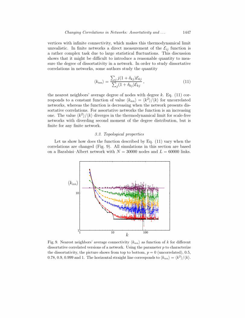
Let us show how does the function described by Eq. (11) vary when thecorrelations are changed (Fig. 9). All simulations in this section are basedon a Barabási–Albert network with N = 30000 nodes and L = 60000 links.

1 10 1001

10

〈knn〉

k

Fig. 9. Nearest neighbors’ average connectivity 〈knn〉 as function of k for different

dissortative correlated versions of a network. Using the parameter p to characterize

the dissortativity, the picture shows from top to bottom, p = 0 (uncorrelated), 0.5,

0.78, 0.9, 0.999 and 1. The horizontal straight line corresponds to 〈knn〉 = 〈k2〉/〈k〉.


We see in Fig. 9 that 〈knn〉 stays constant and is equal to 〈knn〉 = 〈k2〉/〈k〉for uncorrelated network (Eq. (1)). However, when the correlations aremodified by the increase of the parameter p, this flat curve is transformedinto a decreasing one, indicating the appearance of dissortative correlations.In fact, the larger the value of p, the smaller is 〈knn〉 for k ≫ 1. Thisbehavior corresponds exactly to what is expected. Moreover, since almostall highly connected nodes must be linked with nodes of minimum degree,the curve should exhibit a plateau for k ≫ 1, as well as a high peak forthe minimal value of k = 2. Both properties are revealed in our simulations(lower curve of Fig. 9).

Different dissortative real networks, as for example the Internet, show〈knn〉 ∝ k−ν [11]. Our results, plotted on a double logarithmic scale, do notreproduce this behavior. This means that dissortative networks which arerandom with all other respects do not reproduce all properties of dissortativereal networks. We will, however, remark that real networks are also governedby the metrics of the underlying space, normally our Euclidean physicalspace.

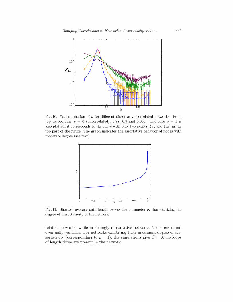
A detailed analysis of strongly dissortative networks shows that theyexhibit properties similar to ones we have described in our ideal dissorta-tive case, such as the assortative correlations among nodes with mediumdegree. Fig. 10 shows E4k as function of k for different dissortative corre-lated networks. We observe, for example, that E45 and E46 increase as thedissortativity grows, in a such a way that E45 > Er

45 as well as E46 > Er46.

This indicates that nodes with degree k = 4 connect preferably with nodeswith degrees k = 5 and k = 6, a clearly indication of assortativity.

Average path length — We now discuss the behavior of the aver-age shortest path length l when the dissortativity of the network increases.Fig. 11 shows l as function of the parameter p. Although the parameter p isan internal parameter of the algorithm and does not immediately representany property of the network, it is clear that any reasonably defined degreeof dissortativity has to be an increasing function of p. Fig. 11 confirms thatthe average path length l always grows when the dissortativity of the net-work increases. At variance with the assortative case, the increase in l ismoderate, and its maximal value is not much higher than in an uncorrelatednetwork.

It is quite interesting to note the average minimal path length in all cor-related networks studied in this work is larger than one for the uncorrelatedones; in might be that for a fixed degree distribution, the network with theminimum average path length would be exactly an uncorrelated one.

Clustering coefficient — Fig. 12 shows the behavior of the mean clus-tering coefficient C as function of p. Thus, in weakly dissortative networksthe clustering coefficient does not change considerably compared to uncor-


1 10 10010

-6

10-4

10-2

1

E4k

k

Fig. 10. E4k as function of k for different dissortative correlated networks. From

top to bottom: p = 0 (uncorrelated), 0.78, 0.9 and 0.999. The case p = 1 is

also plotted; it corresponds to the curve with only two points (E45 and E46) in the

top part of the figure. The graph indicates the assortative behavior of nodes with

moderate degree (see text).

0 0.2 0.4 0.6 0.8 15

6

7

8

l

p

Fig. 11. Shortest average path length versus the parameter p, characterizing the

degree of dissortativity of the network.

related networks, while in strongly dissortative networks C decreases andeventually vanishes. For networks exhibiting their maximum degree of dis-sortativity (corresponding to p = 1), the simulations give C = 0: no loopsof length three are present in the network.


0 0.2 0.4 0.6 0.8 10

0.001

0.002

0.003

0.004

0.005

C

p

Fig. 12. Mean clustering coefficient C as function of the parameter p.

An analysis of the degree-dependent clustering coefficient C̄(k) showsthat C̄(k) is smaller than in the uncorrelated case but remains practicallyconstant. For perfectly dissortative infinite correlated networks (p = 1) onewould have C̄(k) = 0 for all k.

Tomography — The study of tomography on the dissortative versionsof our original Barabási–Albert network, with N = 30000 nodes, yields in-teresting outcomes. In the Fig. 13(a) we plot 〈k〉l as a function of the shellnumber l. In uncorrelated networks the curve 〈k〉l reaches a maximum valueof 〈k2〉/〈k〉 in the first shell and then it smoothly decreases to 〈k〉 = 2corresponding to the minimum node degree. In a dissortative network thebehavior changes: the value of 〈k2〉/〈k〉 oscillates as a function of l: now,the second shell exhibits a local minimum of 〈k〉2, followed by a maximumfor l = 3, decreases again for shell l = 4, etc. These jumps of the tomo-graphical curve are typical for all dissortative networks. The explanation isnot complicated. Using Eq. (10), and supposing as a first approximationthat there exists a large probability that a link leaving a node of degree nenters a node with “opposite” degree (i.e., if n is large then k must be small,and vice versa), one can show that the calculation of the mean, 〈k〉2, yields〈k〉2 < 〈k〉r2 (note that for dissortative networks the number of short loops issmall). Now, if the second shell possesses a large number of lowly connectednodes, the third shell must then be full of highly connected nodes, becauseof the dissortative tendency of nodes to connect. For the same reason theshell l = 4 must contain mostly nodes with small degree, etc.

Thus, dissortative correlations produce networks where the propagat-ing agent more readily reaches nodes with small degree than in uncorrelatedones. In this networks the lowly connected nodes do not form the ”periphery”of the network, and play a more important role in the spreading phenomena,since they represent bridges between the highly connected ones. The periph-


0

4

8

12

16

0 2 4 6 8 10 12 140

0.2

0.4

0.6

0.8

1

〈k〉

n̄

l

(a)

(b)

Fig. 13. (a) Average degree 〈k〉l as function of the number of the shell l. From

top to bottom (or from more peaked to more smooth): p = 1, 0.999, 0.9 and 0

(uncorrelated). (b) n̄(l) = (∑l

i=0

∑

r,k Ni,r(k))/(∑

r,k,i Ni,r(k)) as function of the

shell number l.

ery of the network consists of a large fraction of the nodes of medium degree,which are the last ones to be affected by the spreading agent. Fig. 13(b)shows the cumulative distribution of the average number of nodes per shell

n̄(l) =

∑li=0

∑

r,k Ni,r(k)∑

r,k,i Ni,r(k)(12)

as function of the shell number l. We note that the average path length in-creases when the degree of dissortativity grows and we can offer a qualitative


explanation for this result. We note that the difference between the curvesappears starting from the shell l = 3. Under dissortative mixing a lot ofnodes with small degree, located in the second shell, are connected to nodeswith high degree in the third shell. The inverse is, however, not true sincethe number of highly connected nodes is small. Starting from a smaller num-ber of nodes in the third shell (in comparison to an uncorrelated networks)hinders reaching a large number of further nodes and leads to a weaker pop-ulation of the fourth shell, etc. A careful observation of the curves supportsthis argument: note also that the slope of the lines is smaller when passingfrom an even shell to a odd shell than when changing from an odd to aneven one.

Another important property of dissortative networks compared to theirassortative counterparts is that they always remain fully connected, inde-pendently of their degree of dissortativity. Our simulations show that evenextremely dissortative networks (p = 1) are composed of a single connectedcluster.

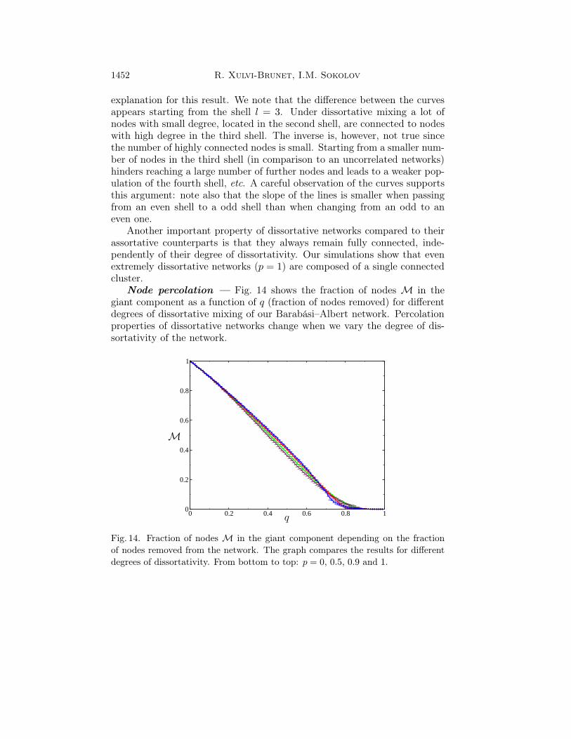
Node percolation — Fig. 14 shows the fraction of nodes M in thegiant component as a function of q (fraction of nodes removed) for differentdegrees of dissortative mixing of our Barabási–Albert network. Percolationproperties of dissortative networks change when we vary the degree of dis-sortativity of the network.

0 0.2 0.4 0.6 0.8 10

0.2

0.4

0.6

0.8

1

M

q

Fig. 14. Fraction of nodes M in the giant component depending on the fraction

of nodes removed from the network. The graph compares the results for different

degrees of dissortativity. From bottom to top: p = 0, 0.5, 0.9 and 1.


Although the differences between them and uncorrelated networks arenot as large as in the assortative case, they could be important. Simulationsshow that as the dissortativity grows the robustness of the networks forsmall and moderate values of q increases. However, when q exceeds somecharacteristic value, the network tends to break more rapidly. While weaklydissortative networks exhibit a percolation behavior quite similar to one ofuncorrelated ones, the behavior of strongly correlated networks seems to bedifferent. However, our simulations do not allow us to make a definitive onthe existence of a real percolation transition in such networks.

4. Conclusions

We present two algorithms based on the idea of rewiring of the preex-isting network which are capable to change correlations in a network andproduce assortative or dissortative mixing leaving all other properties of thenetwork random. Both algorithms do not change the degree distribution ofthe network and avoid creating of multiple and self-connections. The algo-rithms are governed by a single parameter, p, whose variation changes thedegree of assortativity (dissortativity) of the network to a desired amount.Using the algorithms we show that correlations have a drastic influence onthe topological properties of networks. Assortative networks tend to formhighly connected groups of nodes with similar degree which results in anincrease of the average path length and clustering coefficient when the as-sortativity grows. The study of tomography and percolation on assortativenetworks shows that their transport properties differ from ones for uncorre-lated networks. In dissortative networks, the tendency of hubs to connectnodes with low degree also produce changes in the topology; in comparison touncorrelated networks they exhibit larger average path lengths and smallerclustering coefficients. All our results are pertinent to networks which do notexhibit any other correlations that the ones put by their mixing property.We have to note that the real ones might have also other types of correla-tions, and therefore, other statistical properties; geographical restrictions orsimply peculiar properties of certain nodes may play an important role too.

IMS uses the possibility to thank the Fonds der Chemischen Industriefor the partial financial support.


REFERENCES

[1] L.M. Sander, C.P. Warren, I.M. Sokolov, C. Simon, J. Koopman, Math. Biosci.180, 293 (2002).

[2] L.M. Sander, C.P. Warren, I.M. Sokolov, Physica A 325, 1 (2003).

[3] L. Hufnagel, D. Brockmann, T. Geisel, Proc. Natl. Acad. Sci. USA 101, 15124(2004).

[4] R. Albert, A.-L. Barabási, Rev. Mod. Phys. 74, 47 (2002).

[5] S.N. Dorogovtsev, J.F.F. Mendes, Adv. Phys. 51, 1079 (2002).

[6] F. Liljeros, C.R. Edling, L.A.N. Amaral, H.E. Stanley, Y. Aberg, Nature 411,907 (2001).

[7] M.E.J. Newman, Phys. Rev. E67, 026126 (2003).

[8] M.E.J. Newman, Phys. Rev. Lett. 89, 208701 (2002).

[9] A. Vázquez, M. Boguñá, Y. Moreno, R. Pastor-Satorras, A. Vespignani, Phys.Rev. E67, 046111 (2003).

[10] A. Capocci, G. Caldarelli, P. De Los Rios, Phys. Rev. E68, 047101 (2003).

[11] R. Pastor-Satorras, A. Vázquez, A. Vespignani, Phys. Rev. Lett. 87, 258701(2001).

[12] A. Trusina, S. Maslov, P. Minnhagen, K. Sneppen, Phys. Rev. Lett. 92, 178702(2004).

[13] M.E.J. Newman, J. Park, Phys. Rev. E68, 036112 (2003).

[14] J. Berg, M. Lässig, Phys. Rev. Lett. 89, 228701 (2002).

[15] K.-I. Goh, E. Oh, B.Kahng, D. Kim, Phys. Rev. E67, 017101 (2003).

[16] S. Maslov, K. Sneppen, Science 296, 910 (2002).

[17] P.L. Krapivsky, S. Redner, Phys. Rev. E63, 066123 (2001).

[18] S.N. Dorogovtsev, Phys. Rev. E69, 027104 (2004).

[19] D.S. Callaway, J.E. Hopcroft, J. M. Kleinberg, M.E.J. Newman, S.H. Strogatz,Phys. Rev. E64, 041902 (2001).

[20] J. Park, M.E.J. Newman, Phys. Rev. E68, 026112 (2003).

[21] M. Boguñá, R. Pastor-Satorras, A. Vespignani, Phys. Rev. Lett. 90, 028701(2003).

[22] V.M. Eguíluz, K. Klemm, Phys. Rev. Lett. 89, 108701 (2002).

[23] M. Boguñá, R. Pastor-Satorras, Phys. Rev. 66, 047104 (2002).

[24] N. Schwartz, R. Cohen, D. ben-Avraham, A.-L. Barabási, S. Havlin, Phys.Rev. E66, 015104 (2002).

[25] A. Vázquez, Y. Moreno, Phys. Rev. E67, 015101 (2003).

[26] Y. Moreno, J.B. Gómez, A.F. Pacheco, Phys. Rev. E68, 035103 (2003).

[27] S. Maslov, K. Sneppen, A. Zaliznyak, Physica A 333, 529 (2004).

[28] A. Ramezanpour, V. Karimipour, A. Mashaghi, Phys. Rev. E67, 046107(2003).


[29] R. Xulvi-Brunet, W. Pietsch, I. M. Sokolov, Phys. Rev. E68, 036119 (2003).

[30] M. Boguñá, R. Pastor-Satorras, Phys. Rev. E68, 036112 (2003).

[31] I. Farkas, I. Derényi, G. Palla, T. Vicsek, Lect. Notes Phys. 650, 163 (2004).

[32] A.-L. Barabási, R. Albert, Science 286, 509 (1999).

[33] R. Xulvi-Brunet, I.M. Sokolov, Phys. Rev. E70, 066102 (2004).

[34] L.M. Sander, C.P. Warren, I.M. Sokolov, Phys. Rev. E66, 056105 (2002).

[35] R. Cohen, K. Erez, D. ben-Avraham, S. Havlin, Phys. Rev. Lett. 85, 4626(2000).

[36] R. Cohen, D. ben-Avraham, S. Havlin, Phys. Rev. E66, 036113 (2002).

[37] M.E.J. Newman, I. Jensen, R.M. Ziff, Phys. Rev. E65, 021904 (2002).

CHANGING CORRELATIONS IN NETWORKS: ASSORTATIVITY …

Documents

Transcript of CHANGING CORRELATIONS IN NETWORKS: ASSORTATIVITY …