Changbo Chen1 Sviatoslav Covanov2 Farnam Mansouri2

Marc Moreno Maza2 Ning Xie2 Yuzhen Xie2

1Chinese Academy of Sciences2University of Western Ontario

ISSAC 2014 Software demoJuly 23, 2014

1 / 39

Plan

1 Overview

2 Fast Fourier Transform

3 ModularPolynomial

4 IntegerPolynomial

5 RationalNumberPolynomial

6 Conclusion

2 / 39

Background

Reducing everything to multiplication

Polynomial multiplication and matrix multiplication are at the core ofmany algorithms in symbolic computation.Algebraic complexity is often estimated in terms of multiplication timeAt the software level, this reduction is also common (Magma, NTL)Can we do the same for fork-join-multithreaded algorithms?

Building blocks in scientific software

The Basic Linear Algebra Subprograms (BLAS) is an inspiring andsuccessful project providing low-level kernels in linear algebra, used byLINPACK, LAPACK, MATLAB, Mathematica, Julia (among others).Other BB’s successful projects: FFTW, SPIRAL (among others).The GNU Multiple Precision Arithmetic Library project plays a similarrole for rational numbers and floating-point numbers.No symbolic computation software dedicated to sequential polynomialarithmetic managed to play the unification role of the BLAS.Could this work in the case of hardware accelerators?

3 / 39

BPAS Mandate (1/2)

Functionalities

Level 1: basic arithmetic operations that are specific to a polynomialrepresentation or a coefficient ring: multi-dimensional FFTs/TFTs,univariate real root isolationLevel 2: basic arithmetic operations for dense or sparse polynomialswith coefficients in Z, Q or Z/pZ.Level 3: advanced arithmetic operations taking as input azero-dimensional regular chains: normal form of a polynomial,multivariate real root isolation.

4 / 39

BPAS Mandate (2/2)

Targeted architectures

Multi-core processors with code written in CilkPlus or OpenMP. OurMeta Fork framework performs automatic translation between thetwo as well as conversions to C/C++.Graphics Processing Units (GPUs) with code written in CUDA,provided by CUMODP.Unifying code for both multi-core processors and GPUs is conceivable(see the SPIRAL project) but highly complex (multi-core processorsenforce memory consistency while GPUs do not, etc.)

5 / 39

Design

Algorithm choice

Level 1 functions (n-D FFTs/TFTs) are highly optimized in terms oflocality and parallelism.Level 2 functions provide a variety of algorithmic solutions for a givenoperation (polynomial multiplication, Taylor shift, etc.)Level 3 functions combine several Level 2 algorithms for achieving agiven task.

Implementation techniques

At Level 1, code generation at installation time (auto-tuning) is used.At Level 2, the user can choose between algorithms minimizing workand algorithms maximizing parallelism.At Level 3, this leads to adaptive algorithms that select appropriateLevel 2 functions depending on available resources (number of cores,input data size).

6 / 39

Organization

Developer view point

Source tree has two branches: 32bit and 64bit arithmetic with largebodies of common codeFour sub-projects: ModularPolynomial, IntegerPolynomial,RationalNumberPolynomial and Polynomial.For the former three, the base ring is known at compile time while thelatter provides polynomial arithmetic over an arbitrary BPAS ring.Python scripts generate 1-D FFT code at installation time.Dense representations, SLPs and sparse representations are available.

User view point today

Only the 64bit arithmetic branch, but full access to each sub-project.Regression tests and benchmark scripts are also distributed.Documentation is generated by doxygen.A manually written documentation is work in progress.

7 / 39

User interface (1/2)

Figure: A snapshot of BPAS algebraic data structures.

8 / 39

User interface (2/2)

Figure: A snapshot of BPAS code.

9 / 39

Plan

1 Overview

2 Fast Fourier Transform

3 ModularPolynomial

4 IntegerPolynomial

5 RationalNumberPolynomial

6 Conclusion

10 / 39

BPAS 1-D FFT

BPAS 1-D FFTs code is optimized in terms of cache complexity andregister usage, following principles introduced by FFTW and SPIRAL.

The FFT of a vector of size n is computed in a divide-and-conquermanner until the vector size is smaller than a threshold, at whichpoint FFTs are computed using a tiling strategy.

At compile time, this threshold is used to generate and optimize thecode. For instance, the code of all FFTs of size less or equal toHTHRESHOLD are decomposed into blocks (typically performing FFTson 8 or 16 points) for which straight-line program (SLP) machinecode is generated by python scripts.

Instruction level parallelism (ILP) is carefully considered: vectorizedinstructions are explicitly used (SSE2, SSE4) and instruction pipelineusage is highly optimized.

Other environment variables are available for the user to controldifferent parameters in the code generation.

11 / 39

1-D FFT Benchmarks

Figure: One-dimensional modular FFTs: Modpn vs BPAS.

12 / 39

Plan

1 Overview

2 Fast Fourier Transform

3 ModularPolynomial

4 IntegerPolynomial

5 RationalNumberPolynomial

6 Conclusion

13 / 39

2-D TFT versus 2-D FFT

2048 2560

3072 3584

4096 2048 2560

3072 3584

4096

0.3

0.4

0.5

0.6

0.7

0.8

0.9

1

1.1

Time(s)

2-D FFT method on 8 cores (0.806-0.902 s, 7.2-7.3x speedup)2-D TFT method on 8 cores (0.309-1.08 s, 6.8-7.6x speedup)

d1+d1’+1d2+d2’+1

Time(s)

Figure: Timing of bivariate multiplication for input degree range of [1024, 2048)on 8 cores.

14 / 39

Balanced Dense Multiplication over Z/pZ

32768 40960

49152 57344

65536 32768

40960 49152

57344 65536

0

2

4

6

8

10

12

14

16

Time

Ext.+Contr. of 4-D to 2-D TFT on 1 core (7.6-15.7 s)Kronecker’s substitution of 4-D to 1-D TFT on 1 core (6.8-14.1 s)

Ext.+Contr. of 4-D to 2-D TFT on 2 cores (1.96x speedup, 1.75x net gain)Ext.+Contr. of 4-D to 2-D TFT on 16 cores (7.0-11.3x speedup, 6.2-10.3x net gain)

d1 (d2=d3=d4=2)d1’ (d2’=d3’=d4’=2)

Time

15 / 39

Plan

1 Overview

2 Fast Fourier Transform

3 ModularPolynomial

4 IntegerPolynomial

5 RationalNumberPolynomial

6 Conclusion

16 / 39

Integer polynomial multiplication

Five different integer polynomial multiplication algorithms areavailable:

Schonhage-Strassen, 8-way Toom-Cook, 4-way Toom-Cook,divide-and-conquer plain multiplication and the two-convolutionmethod.

The first one has optimal work (among the five) but is purely serialdue to the difficulties of parallelizing 1D FFTs on multicore processors.

The next three algorithms are parallelized but their parallelism isstatic, that is, independent of the input data size; these algorithms arepractically efficient when both the input data size and the number ofavailable cores are small, for details.

The fifth algorithm relies on modular 2D FFTs which are computed bymeans of the row-column scheme; this algorithm delivers a highscalability and can fully utilize fat computer nodes.

17 / 39

KS+GMP: Reduction to GMP via Kronecker substitution

f (x) :=n∑

i=0fix

i , g(x) :=m∑i=0

gixi , h(x) = f (x)× g(x) =

n+m−1∑i=0

hixi

Assume 0 ≤ fi < Hf and 0 ≤ j < m for all fi ’s and gj ’s.

Then we have: 0 ≤ hk < min(n,m)HfHg + 1, for 0 ≤ k < n + m − 1.Thus B := dlog2 min(n,m)HfHg + 1e is the maximum number of bitsrequired for representing a coefficient of the result.

If f or g has a negative coefficient we use a “two-complement”-trick.

Steps

1 Evaluation: Zf =n∑

i=0fi2

iB , Zg =m∑i=0

fi2iB

2 Multiplying: Zh = Zf × Zg using GMP library.

3 Unpacking: hi s from Zh =n+m−1∑i=0

hi2iB

Analysis

Work is in O(s log(s)log(log(s))). s is the maximum bit size of f or g(Schonhage & Strassen). But no parallelism and modest data locality.

18 / 39

DnC+KS+GMP: GMP Reduction via KS and distributivity

Steps

1 Divide: f (x) = f0(x) + xn/2f1(x), g(x) = g0(x) + xn/2g1(x)2 Execute 4 sub-problems recursively.

I Store f0 × g0 and f1 × g1 in the result array.I Store f0 × g1 and f1 × g0 in auxiliary arrays.

3 Add the auxiliary arrays to the result.4 Use (one or) two DnC levels, then use the KS+GMP algorithm.

Analysis

Work is in O(s log(s)log(log(s))). But, w.r.t. pure KS+GMP, the constanthas increased by approximately by 4. However, parallelism is close to 16.

19 / 39

k-way Toom-Cook and reduction to GMP (1/4)

1 Division: Write f (x) = f0(x) + xn/k f1(x) + . . .+ x (k−1)n/k fk−1(x)and g(x) = g0(x) + xn/kg1(x) + . . .+ x (k−1)n/kgk−1(x)

2 Conversion: Set X = xn/k and apply KS to the fi ’s and gj ’s.Obtaining F (X ) = Zf0 + Zf1X + . . .+ Zfk−1

X k−1 andG (X ) = Zg0 + Zg1X + . . .+ Zgk−1

X k−1.

3 Evaluation: Evaluate f , g at 2k − 1 points: (0,X1, . . . ,X2k−3,∞)

4 Multiplying: (w0, . . . ,w2k−2) = (F (0) · G (0), . . . ,F (∞) · G (∞))

5 Interpolation: recover (Zh0 ,Zh1 , . . . ,Zh2k−2) where:

H(X ) = f (X )g(X ) = Zh0 + Zh1X + . . .+ Zh2k−2X 2k−2.

6 Conversion: recover polynomial coefficients from Zh0 , . . . , . . . ,Zh2k−2.

Obtaining h(x) = h0(x) + xn/kh1(x) + . . .+ x (2k−2)n/kh2k−2(x).

7 Merge: Add intermediate results to the final result.

20 / 39

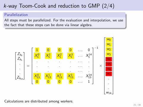
k-way Toom-Cook and reduction to GMP (2/4)

Parallelization

All steps must be parallelized. For the evaluation and interpolation, we usethe fact that these steps can be done via linear algebra.

Zh0

Zh1

.

.

.Zh14

=

1 0 0 0 . . . 0

X 01 X 1

1 X 21 X 3

1 . . . X 141

. . . . . . . .

. . . . . . . .

. . . . . . . .

X 013 X 1

13 X 213 X 3

13 . . . X 1413

0 0 0 0 . . . 1

−1

×

w0

w1

w2

w3

w4

w5

w6

w7

.

.

.w14

Calculations are distributed among workers.

21 / 39

k-way Toom-Cook and reduction to GMP (3/4)

Analysis

Work in O(s log(s)log(log(s))). W.r.t. pure KS+GMP, for k = 8, theconstant has increased approximately by 2 for s = 224.However, parallelism is about 7 and 13 when k = 4 and k = 8, resp.In the 3 tables below, a 12-core (Intel Xeon) is used.In the last one, we have

√s = 8192.

Toom-8 Profiled results√s Div. & Conv. Eval. Mul. Inter. Con. & Merge

16384 10% 8% 44% 25% 9%32768 9% 9% 43% 27% 10%65536 8% 8% 45% 28% 9%

Toom-4 Profiled results√s Div. & Conv. Eval. Mul. Inter. Con. & Merge

16384 13% 3% 57% 11% 13%32768 12% 3% 61% 11% 12%65536 8% 2% 66% 10% 11%

22 / 39

k-way Toom-Cook and reduction to GMP (4/4)

Algorithm Timing Work Span Work/serial Span/serialKS (Ser.) 1 16781990263 16781990263 1 1

DnC 15.86 67222430575 4237755216 4 0.25Toom-4 6.42 28289430113 4382572841 1.68 0.26Toom-8 11.26 24449014227 2023790230 1.45 0.12

Notes

Span of Toom-8 is the best, 12 % of the KS→ It should be much better on better machines.Work of the Toom-8 & Toom-4 are more than KS, but much betterthan DnC.But for Toom-8 and Toom-4, GMP-multiplication is not the dominantpart.Hence, we need an algorithm which can scale on fatter nodes.

23 / 39

Two-convolution method (1/7)

Specifications

Input: a(y), b(y) ∈ Z[y ] with max(deg(a),deg(b) < d and N0 themaximum bit size of a coefficient among a(y) and b(y).Intention: a(y), b(y) are dense in the sense that most coefficientshave a size in the order of N0.Output: c(y) = a(y)b(y).

Theorem

Let w be the number of bits of a machine word. There exist positiveintegers N,K ,M, with N = K M and M ≤ w , such that the integer N isw -smooth (and so is K ), we have N0 < N ≤ N0 +

√N0 and the following

algorithm for multiplying a(y), b(y) hasa work of O(d K log2(d K )(log2(d K ) + 2M)) word operations,a span of O(K log2(d) log2(d K )) word operations and,incurs O(ddN/wLe+ d(log2(d K ) + 2M)e dK/L) cache misses,

24 / 39

Two-convolution method (2/7)

Principle

1 Convert-in: convert the integer coefficients of a(y), b(y) to Z[x ],thus converting a(y), b(y) to A(x , y),B(x , y) s.t. for some β ∈ Z:

1 a(y) = A(β, y) and b(y) = B(β, y),2 deg(A, y) = deg(a) and deg(B, y) = deg(b),3 max(bitsize(a),bitsize(b)) ∈ Θ(max(bitsize(a),bitsize(b)))

Let m > 4H be an integer, where H is the maximum absolute valueof a coefficient of the integer polynomial C (x , y) := A(x , y)B(x , y).

2 Compute: m and A(x , y),B(x , y) are constructed such that1 the polynomials C+(x , y) := A(x , y)B(x , y) mod 〈xK + 1〉 and

C−(x , y) := A(x , y)B(x , y) mod 〈xK − 1〉 are computed over Z/mZvia FFT techniques

2 meanwhile the following equation holds over Z:

C (x , y) =C+(x , y)

2(xK − 1) +

C−(x , y)

2(xK + 1).

3 Convert-out: Compute u(y) := C+(β, y) and v(y) := C−(β, y)

over Z. Then, deduce c(y) := u(y)+v(y)2 + −u(y)+v(y)

2 2N over Z.25 / 39

Two-convolution method (3/7)

Figure: Multiplication scheme for dense univariate integer polynomials.

26 / 39

Two-convolution method (4/7)

Principle (recall)

1 Convert-in: convert a(y), b(y) to A(x , y),B(x , y) s.t. for someβ ∈ Z we have a(y) = A(β, y) and b(y) = B(β, y).

2 Let m > 4H where H := || C (x , y) ||∞ withC (x , y) := A(x , y)B(x , y).

3 Compute:C+(x , y) := A(x , y)B(x , y) mod 〈xK + 1〉 andC−(x , y) := A(x , y)B(x , y) mod 〈xK − 1〉 over Z/mZ.

4 Convert-out: Compute u(y) := C+(β, y) and v(y) := C−(β, y)

over Z. Then, deduce c(y) := u(y)+v(y)2 + −u(y)+v(y)

2 2N over Z.

Remarks

For polynomials with size in the Giga-bytes, we can choose m < 2w .Thus each of C+(x , y) and C−(x , y) requires at most two 2-DFFT/TFT over a prime field with characteristic of machine word size.Convert-in and Convert-out are done only with addition and shiftoperations on byte vectors: GMP is not used.The cache complexity of this process is proved to be optimal. 27 / 39

Two-convolution method (5/7)√s ConvertIn TwoConvolution ConvertOut Total

2048 0.038 0.106 0.042 0.1954096 0.039 0.23 0.107 0.398192 0.119 0.895 0.267 1.298

16384 0.248 3.705 0.665 4.64332768 0.943 16.272 4.217 21.496

Table: Using 2 primes on a 48-core AMD Opteron node.

√s ConvertIn TwoConvolution ConvertOut Total

2048 0.037 0.113 0.052 0.2274096 0.028 0.206 0.103 0.3648192 0.07 0.652 0.307 1.059

16384 0.224 2.71 0.73 3.69832768 0.943 11.796 4.174 16.978

Table: Using 3 primes on a 48-core AMD Opteron node.

This about four faster than Toom-8 at√s = 8192.

28 / 39

Two-convolution method (6/7)

Figure: Dense integer polynomial multiplication: BPAS vs FLINT vs Maple 18.

29 / 39

Two-convolution method (7/7)

Figure: Dense integer polynomial multiplication: BPAS vs FLINT vs Maple 18.

30 / 39

Plan

1 Overview

2 Fast Fourier Transform

3 ModularPolynomial

4 IntegerPolynomial

5 RationalNumberPolynomial

6 Conclusion

31 / 39

Univariate Real Root Isolation Algorithm: Find Roots

Input: A univariate squarefree polynomial f (x) = cd xd + · · ·+ c1 x + c0

with rational number coefficients

Output: A list of pairwise disjoint intervals [a1, b1], . . . , [ae , be ] withrational endpoints such that

each [ai , bi ] contains one and only one real root of f (x);

if ai = bi , the real root xi = ai (bi ); otherwise, the real rootai < xi < bi (f (x) doesn’t vanish at either endpoint).

Figure: An example of input / output

32 / 39

Real Root Isolation (Collins-Vincent-Akritas Algorithm)

Algorithm 1: NumberInZeroOne(p)

Input: a squarefree univariate polynomial pOutput: number of real roots of p in (0, 1)begin

p1 := xnp(1/x); p2 := p1(x + 1)let d be the number of sign variations of the coefficients of p2if d ≤ 1 then return dp1 := 2np(x/2); p2 := p1(x + 1)if x | p2 then m := 1 else m := 0m′ := NumberInZeroOne(p1)m := m + NumberInZeroOne(p2)return m + m′

end

The Taylor shift f (x) 7−→ f (x + 1) operation is at the core of the abovealgorithm for real root isolation (counting).

33 / 39

Univariate Taylor Shift: Parallel Horner’s Method

Horner’s method

We compute g(x) = f0 + (x + 1) (f1 + · · ·+ (x + 1) fd) in n steps

g (0) = fd , g(i) = (x + 1) g (i−1) + fd−i for 1 ≤ i ≤ d ,

and obtain g = g (d).One can represent this computation in a Pascal’s Triangle.

Given an example f (x) = a3 x3 + a2 x

2 + a1 x + a0, we have, in Horner’s rule as follows.

0 0 0 0↓ ↓ ↓ ↓

a3 → + → + → + → + → c3↓ ↓ ↓

a2 → + → + → + → c2↓ ↓

a1 → + → + → c1↓

a0 → + → c0

Thus, g(x) = f (x + 1) = c3 x3 + c2 x

2 + c1 x1 + c0. For instance, we can parallelize theaddition a1 + a2, a2 + a3 and a3 + 0, and so on.

34 / 39

Univariate Taylor Shift: Parallel Divide & Conquer Method

Divide & conquer method

We assume that d + 1 = 2` is a power of two. In a precomputation stage, we compute(1 + x)2

ifor 0 ≤ i < `. In main stage, with polynomials f (0), f (1) ∈ Q[x ] of degree less

than d+12 , we compute

g(x) = f (0)(x + 1) + (x + 1)(d+1)/2 f (1)(x + 1),

where we compute f (0)(x + 1) and f (1)(x + 1) recursively.

We parallelize each univariate polynomial multiplication by a DnC method. For example,

35 / 39

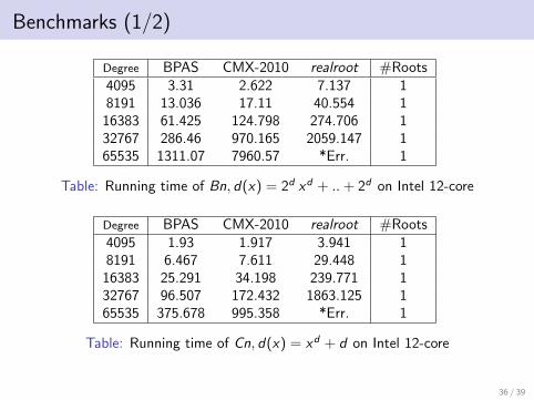
Benchmarks (1/2)

Degree BPAS CMX-2010 realroot #Roots4095 3.31 2.622 7.137 18191 13.036 17.11 40.554 1

16383 61.425 124.798 274.706 132767 286.46 970.165 2059.147 165535 1311.07 7960.57 *Err. 1

Table: Running time of Bn, d(x) = 2d xd + ..+ 2d on Intel 12-core

Degree BPAS CMX-2010 realroot #Roots4095 1.93 1.917 3.941 18191 6.467 7.611 29.448 1

16383 25.291 34.198 239.771 132767 96.507 172.432 1863.125 165535 375.678 995.358 *Err. 1

Table: Running time of Cn, d(x) = xd + d on Intel 12-core

36 / 39

Benchmarks (2/2)

Size BPAS CMX-2010 realroot #RootsBnd 4096 4.003 5.125 4.955 1

8192 11.025 25.228 23.754 116384 43.498 127.412 159.245 132768 176.351 609.513 1,011.872 165536 701.682 4,695.31 9,741.249 1

Cnd 4096 0.704 1.209 1.699 18192 1.533 5.228 10.899 1

16384 5.086 25.296 109.420 132768 18.141 125.902 816.134 165536 66.436 664.438 7,526.428 1

Chebycheff 2048 608.738 594.82 1,378.444 20474096 8,194.06 10,014 35,880.069 4095

Laguerre 2048 1,336.14 1,324.33 3,706.749 20474096 20,727.9 23,605.7 91,668.577 4095

Wilkinson 2048 630.481 614.94 1,031.36 20474096 9,359.25 10,733.3 26,496.979 4095

Table: Running times on AMD 48-core

37 / 39

Plan

1 Overview

2 Fast Fourier Transform

3 ModularPolynomial

4 IntegerPolynomial

5 RationalNumberPolynomial

6 Conclusion

38 / 39

Summary

www.bpaslib.org

39 / 39