arX

iv:1

604.

0203

4v2

[as

tro-

ph.G

A]

9 A

pr 2

016

Prepared for submission to JCAP

Chandrasekhar’s Dynamical Friction

and non-extensive statistics

J. M. Silva,a J. A. S. Lima,b R. E. de Souza,b A. Del Popolo,c,d,e

Morgan Le Delliou,f Xi-Guo Leeg

aCentro de Formacao de Professores da UFCG, Cajazeiras, PBbInstituto de Astronomia, Geofısica e Ciencias Atmosfericas, USP, 05508-900 Sao Paulo, SP,Brasil

cDipartimento di Fisica e Astronomia, University Of Catania, Viale Andrea Doria 6, 95125Catania, Italy

dINFN sezione di Catania, Via S. Sofia 64, I-95123 Catania, ItalyeInternational Institute of Physics, Universidade Federal do Rio Grande do Norte, 59012-970Natal, Brazil

f Instituto de Fısica Teorica, Universidade Estadual de Sao Paulo (IFT-UNESP),Rua Dr. Bento Teobaldo Ferraz 271, Bloco 2 - Barra Funda, 01140-070 S˜ao Paulo, SPBrazil

gInstitute of Modern Physics, Chinese Academy of Sciences,Post Office Box 31, Lanzhou 730000, People’s Republic of China

Abstract. The motion of a point like object of mass M passing through the backgroundpotential of massive collisionless particles (m << M) suffers a steady deceleration nameddynamical friction. In his classical work, Chandrasekhar assumed a Maxwellian velocitydistribution in the halo and neglected the self gravity of the wake induced by the gravitationalfocusing of the mass M . In this paper, by relaxing the validity of the Maxwellian distributiondue to the presence of long range forces, we derive an analytical formula for the dynamicalfriction in the context of the q-nonextensive kinetic theory. In the extensive limiting case(q = 1), the classical Gaussian Chandrasekhar result is recovered. As an application, thedynamical friction timescale for Globular Clusters spiraling to the galactic center is explicitlyobtained. Our results suggest that the problem concerning the large timescale as derived bynumerical N -body simulations or semi-analytical models can be understood as a departurefrom the standard extensive Maxwellian regime as measured by the Tsallis nonextensiveq-parameter.

Keywords: Dynamical Friction– Nonextensivity– Globular Clusters

Contents

1 Introduction 1

2 Dynamical Friction and Nonextensive Effects 4

3 Decay of Globular Orbits 7

3.1 Comparison with N-body simulations 10

4 Conclusions 13

1 Introduction

The analysis of the dynamics of stellar systems such as globular clusters or clusters of galaxieshas shown that the gravitational stochastic force plays a fundamental role in their evolution(Chandrasekhar & von Newman 1942, 1943; Kandrup 1980; Ardi & Inagaki 1999). In thesesystems the stochastic force, arising from statistical fluctuations in the number of neighbors ofa test star, perturbs the stars orbits from the orbits they would have if the density distributionin the system were perfectly smooth. The existence of the stochastic force is due to thediscreteness of gravitational systems, i.e. to the fact that the mass is concentrated intodiscrete objects like stars. The first consequence produced by the stochastic force is theexistence of a frictional force that implies a preferential deceleration of a particle in thedirection of motion (Chandrasekhar & von Newman 1942, 1943).

The study of the statistics of the fluctuating gravitational force in infinite homogeneoussystems was pioneered by Chandrasekhar & Von Neumann in two classical papers (Chan-drasekhar & Von Neumann 1942, 1943). Their analysis of the fluctuating gravitational fieldwas formulated statistically, in a treatment related to the so-called Holtsmark’s distribution(Holtsmark 1919), by W (F), which gives the probability that a test star is subject to a forceF in the range F+dF, and by the distribution W (F+dF) which gives the speed of fluctu-ations, i.e. the joint probability that the star experiences a force F and a rate of changef=dF/dt. From such statistical treatment, Chandrasekhar showed the emergence of a dy-namical friction (DF) force, a dissipative force connected to the fluctuations in the medium,thus an aspect of the fluctuation-dissipation relation (see also Bekenstein & Maoz 1992).

Chandrasekhar’s famous formula was not obtained in the general statistical framework(Chandrasekhar & von Newman 1942, 1943) because of the mathematical complexity ofthe scheme, but rather in another paper (Chandrasekhar 1943), restricted to a two-pointinteraction scheme, and his aim to re-derive this formula only from his general theory ofstochastic forces has never been realized.

In that paper (Chandrasekhar 1943), the formula was obtained assuming that a pointmass moves through an infinite, homogeneous sea of field particles, in the approximation thatbinary encounters dominate. In this case a fraction of the kinetic energy of the incomingobject is transferred to the stellar collisionless population whose distribution was describedby a Maxwellian velocity.

The formula shows that a massive object of mass M such as a Globular Cluster passingthrough a background of non-colliding particles suffers a gravitational force which slows downits motion.

– 1 –

Despite being obtained for an homogeneous and infinite system, neglecting self-gravity(i.e., the interaction between the field particles) (Maoz 1993), and resonant interactionsbetween the background and the infalling body (e.g., Weinberg 1986; Inoue 2009), the DFmechanism is now considered a classical effect in the description and evolution of almost allmany-body astrophysical systems, as it has been applied quite successfully.

Examples of its application involve the formation of stellar galactic nuclei via merging ofold Globular Clusters (GCs) [Tremaine et al. 1975], the transformation from non-nucleateddwarf galaxies into nucleated ones [Oh & Lin 2000], the behavior of radio galaxies in galaxyclusters [Nath 2008], in nonlinear gaseous media [Kin & Kin 2009] and in field particles with amass spectrum [Ciotti 2010]. Traditionally, such investigations were carried out in the frame-work of Newtonian gravity, however, alternative gravity theories like the Modified NewtonianDynamics (MOND) has also been considered [Nipoti et al. 2008].

DF is also of fundamental importance in determining the observed properties of clus-ters of galaxies (White 1976; Kashlinsky 1986,1987; Colafrancesco, Antonuccio-Delogu, DelPopolo 1995) and in the orbital decay of a satellite moving around a galaxy or in the merg-ing scenario (Bontekoe & van Albada 1987; Seguin & Dupraz 1996; Dominguez-Tenreiro &Gomez-Flechoso 1998; Del Popolo & Gambera 1997; Antonuccio-Delogu & Colafrancesco1994).

Finally, the use of such formula speeds up considerably N-body simulations. For ex-ample, self-consistent modeling of the internal dynamics of a 105M⊙ GC requires 107 − 1012

background particles to model the inspiral: smaller mass resolution (i.e., less particles) pro-duces an under-prediction of the dynamical friction force. The dynamical friction formulaallows to skip the calculation of the interaction with the background, and to concentrate onthe calculation of the internal dynamics.

However, Chandrasekhar’s formula suffers from some break downs, such as

a. the evolution of a displaced super massive black hole (Gualandris & Merritt 2008);

b. the overprediction of the infalling timescale in cored systems, the so-called ”core stallingproblem” (see the following);

c. the inadequacy of the formula to describe dynamical friction in head-on encounters(Seguin & Dupraz 1996a);

d. the inaccuracy of the formula to calculate DF in disks1.

It is therefore of utmost importance to have a reliable semi-analytic formula to describeDF in the break down cases.

Improving the treatment of dynamical friction was attempted, following two differentpaths:

A. recalculate dynamical friction starting from a statistical analysis approach, whetherChandrasekhar’s or another. Such approaches comprise:

(1) a Fokker-Planck analysis of binary interaction to estimate the diffusion coefficients(e.g., Rosenbluth, MacDonald & Judd 1957; Binney & Tremaine 1987).

1A better model to describe DF in disks is that of obtained by Binney (1977), modifying Chandrasekhar’stheory

– 2 –

(2) the polarization cloud approach (e.g., Bekenstein & Zamir 1991) recovers Chan-drasekhar’s formula in the case of very massive test particle (Kandrup 1983).

(3) the derivation of frictional effects starting from the interaction of test objects andresonant particles (e.g., Weinberg 1986).

(4) returns on Chandrasekhar’s statistical approach:

i. the Cohen (1975) and Kandrup (1980) two-body approximation with fullstochastic theory, from which Kandrup (1983a,b) reobtained Chandrasekhar’sformula for test particles more massive and slower than background particles.Kandrup (1980) showed the stochastic approach disagree with the formula inthe weak forces limit because the nontrivial role distant field stars play in thestochastic force.

ii. the interaction of a test particle and a background stochastic force, going backto the Chandrasekhar’s statistical theory, in Bekenstein & Maoz (1992), andMaoz (1993), where they found Chandrasekhar’s friction force depends on theglobal structure of the system (Maoz 1993; Del Popolo & Gambera 1999; DelPopolo 2003), in inhomogeneous systems, and is no longer directed oppositeto the test particle’s motion.

B. correct Chandrasekhar’s formula to give improved predictions in peculiar situations.

Although approach B is theoretically more limited than approach A, for lack of funda-mental insight and design for a given peculiar situation, it retains value in actionable power,as the path A, despite clarifying the limits of Chandrasekhar’s formula with some improvedformulas (e.g., Maoz 1993), did not find a complete solution to the dynamical friction prob-lem.

For example, approach B can improve the formula to reduce its discrepancy with sim-ulations prediction for timescale of spiraling of objects in a system with cored dark matterhalo of constant density distribution (e.g., Petts, Gualandris & Read 2015), but cannot solvethe problem of evaluation of dynamical friction in head-on encounters.

In this work we will adopt a type B approach and focus on the core stalling problem,i.e. the unability of Chandrasekhar’s formula to predict the stalling of infall of objects incored systems. In the last few years, several authors have related the problem to the DFtimescale (tdf ) of a GC orbiting dwarf galaxies or of infalling satellite galaxies in clusters(Read et al. 2006; Goerdt et al. 2006; Sanchez-Salsedo et al. 2006; Nath 2008; Cowsik et al.

2009; Inoue 2009; Namouni 2010, Gan et al. 2010). In particular, the DF effects for dwarfgalaxies with cored dark matter halo of constant density distribution have been found tobe considerably modified (i.e. not experiencing dynamical friction (Goerdt 2010)). N -bodysimulations [Goerdt et al. 2006, Inoue 2009, Goerdt et al. 2010] have shown that the sinkingtimescale of GCs to the galactic center may exceed the age of the universe, such that theyappear to stall at the edge of the core (Goerdt 2010).

The reason for this stalling is interpreted in Goerdt (2006) as orbit-scattering reso-nance, or corotating state: perturber and background reach a stable state characterized byno angular momentum exchange. Inoue (2009) disagree with Goerdt (2006, 2010) on that in-terpretation. In any case, all simulations agree with the stalling, contrary to Chandrasekhar’sformula. Here we propose a solution based on a proper extension of the underlying statisticalapproach.

– 3 –

The so-called nonextensive statistical approach provides an analytical extension ofBoltzmann-Gibbs (BG) statistical mechanics very suitable to include effects of long-rangeforces and/or mildly out of thermal equilibrium states. This ensemble theory is based on theformulation of a generalized entropy proposed by Tsallis (1988,2009)

Sq = kB1−

∑Wi=1 p

i

1− q, (1.1)

which reduces in the limit q → 1 to the BG entropy SBG = −kB∑W

i=1 pi ln pi, since pi is

the probability of finding the systems in the microstate i, W is the number of microstatesand kB is the Boltzmann constant. However, when the index q 6= 1, the entropy of thesystem is nonextensive, i.e, given two subsystems A and B, the entropy is no more addi-tive in the sense that Sq(A + B) = Sq(A) + Sq(B) + (1 − q)Sq(A)Sq(B). The long-rangeinteractions are associated to the last term on the r.h.s. which accounts for correlationsbetween the subsystems with the index q quantifying the degree of statistical correlations.Such a statistical description has been successfully applied to many complex physical sys-tems ranging from physics to astrophysics and plasma physics, among which: the electrostaticplane-wave propagation in a collisionless thermal plasma (Lima, Silva & Santos 2000), thepeculiar velocity function of galaxies clusters [Lavagno et al. 1998], gravothermal instabil-ity [Taruya & Sakagami 2002], the kinetic concept of Jeans gravitational instability (Lima,Silva & Santos 2002), and the radial and projected density profiles for two large classes ofisothermal stellar systems [Lima & de Souza 2005]. A wide range of physical applicationscan also be seen in Gell-Mann & Tsallis 2004 (see also http://tsallis.cat.cbpf.br/biblio.htmfor an updated bibliography).

In this paper, by assuming that a self-gravitating collisionless gas is described by thenonextensive kinetic theory (Silva et al. 1998; Lima et al. 2001), we derive a new analyticalformula for DF which generalizes the Chandrasekhar result. As an application, the DFtimescale (tdf ) for GCs falling in the galaxies center is derived for the case of a singularisothermal sphere. This result suggest that the long timescales for GCs can be understoodas a departure from the extensive regime.

2 Dynamical Friction and Nonextensive Effects

By following Chandrasekhar (1943), the DF deceleration on a test mass M moving withvelocity vM in a homogeneous and isotropic distribution of identical field particles of massm and number density n0 reads:

dvM

dt= −16π2(ln Λ)G2Mm

∫ vM0 f(v)v2dv

v3MvM, (2.1)

where G is the gravitational constant, m is the mean mass of field stars and f(v) representstheir velocity distribution. The parameter Λ = pmax/pmin depends on the ratio of themaximum (pmax) and minimum (pmin) impact parameters of the encounters contributing togenerate the dragging force.

In the applications of DF, it is usually assumed that the distribution function of thestellar velocity field can be described by a Maxwellian distribution [Binney & Tremaine 2008,Fellhauer 2008]

f(X⋆) =n0

(2πσ2)3/2e−X2

⋆ , (2.2)

– 4 –

where X⋆ = v/√2σ denotes a normalized velocity with σ indicating their dispersion. The

integration of (2.1) results in:

dvM

dt= −4π ln ΛG2Mρ(r)

v3MH1(XM )vM, (2.3)

where ρ(r) = n0m and the function H1(XM ) is given by

H1(XM ) = erf(XM )− 2XM√π

e−X2

M , (2.4)

with erf(XM ) defining the error function as

erf(XM ) =2√π

∫ XM

0e−X2

⋆dX⋆. (2.5)

Now, in order to investigate the nonextensive effects on the Chandrasekhar theory, letus consider that the stellar field obeys the following power-law (Silva, Plastino & Lima 1998,Lima, Silva & Plastino 2001, Lima & de Souza 2005):

f(X⋆) =n0

(2πσ2)3/2Aqeq(X⋆) (2.6)

where the so-called q-exponential is defined by

eq(X⋆) =[

1− (1− q)X2⋆

]1

1−q , (2.7)

and the quantity Aq denotes a normalization constant which depends on the interval of the q-parameter. For values of q < 1, the positiveness of the power argument means that the abovedistribution exhibits a cut-off in the maximal allowed velocities. In this case, all velocitieslie on the interval (0, vmax) and their maximum value is vmax =

√2σ/

√1− q. Taking this

into account one may show that the normalization constant Aq can be written in terms ofGamma functions as follows:

Aq = (1 − q)1/2(5−3q2 )(3−q

2 )Γ( 1

1−q+ 1

2)

Γ( 1

1−q), q < 1

Aq = (q − 1)3/2Γ( 1

q−1)

Γ( 1

q−1−

3

2), q > 1

(2.8)

For generic values of q 6= 1, the DF (2.6) is a power law, whereas for q = 1 it reducesto the standard Maxwell-Boltzmann distribution function (2.2) since A1 → 1 at this limit.

Formally, this result follows directly from the known identity, limd→0(1 + dy)1

d = exp(y)[Abramowitz & Stegun 1972]. The distribution (2.6) is uniquely determined from two sim-ple requirements (Silva et al. 1998): (i) isotropy of the velocity space, and (ii) a suitablenonextensive generalization of the Maxwell factorizability condition, or equivalently, the as-sumption that f(v) 6= f(vx)f(vy)f(vz). The kinetic foundations of the above distributionwere also investigated in a deeper level through the generalized Boltzmann’s equation. In par-ticular, it was also shown that the kinetic version of the Tsallis entropy satisfies an extendedHq-theorem (Lima, Silva & Plastino 2001).

– 5 –

0,2 0,4 0,6 0,8 1 1,2 1,4 1,6 1,8 2 2,2 2,4 2,6 2,8x

0

0,2

0,4

0,6

0,8

1

Hq(x

)

q = 0.80q = 0.90q = 1.00q = 1.10q = 1.20

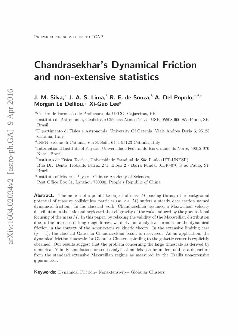
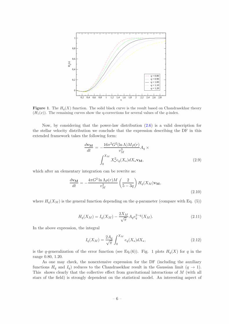
Figure 1. The Hq(X) function. The solid black curve is the result based on Chandrasekhar theory(H1(x)). The remaining curves show the q-corrections for several values of the q-index.

Now, by considering that the power-law distribution (2.6) is a valid description forthe stellar velocity distribution we conclude that the expression describing the DF in thisextended framework takes the following form:

dvM

dt= −16π2G2(ln Λ)Mρ(r)

v3MAq ×

∫ XM

0X2

⋆eq(X⋆)dX⋆vM, (2.9)

which after an elementary integration can be rewrite as:

dvM

dt= −4πG2 ln Λρ(r)M

v3M

(

2

5− 3q

)

Hq(XM )vM,

(2.10)

where Hq(XM ) is the general function depending on the q-parameter (compare with Eq. (5))

Hq(XM ) = Iq(XM )− 2XM√π

Aqe2−qq (XM ). (2.11)

In the above expression, the integral

Iq(XM ) =2Aq√π

∫ XM

0eq(X⋆)dX⋆, (2.12)

is the q-generalization of the error function (see Eq.(6)). Fig. 1 plots Hq(X) for q in therange 0.80, 1.20.

As one may check, the nonextensive expression for the DF (including the auxiliaryfunctions Hq and Iq) reduces to the Chandrasekhar result in the Gaussian limit (q → 1).This shows clearly that the collective effect from gravitational interactions of M (with allstars of the field) is strongly dependent on the statistical model. An interesting aspect of

– 6 –

the above formulae is that the results are given by analytical expressions. In principle,they can be useful for semi-analytical implementations because the easy comparison withthe standard approach (see next section). Naturally, we are also advocating here that theidealized framework based on the Maxwellian distribution (Chandrasekhar 1943) may be inthe root of some theoretical difficulties shown by N -body simulations, like the ones relatedto the decay orbits of GCs.

3 Decay of Globular Orbits

In order to illustrate some consequences of the above derivation, let us now analyze thenonextensive solution for the decaying orbit of a GC in the stellar galactic field. As aGC orbits through the galactic field, it is subject to DF due to its interaction with thestellar distribution. By assuming spherically symmetric star distribution, the dragging forcedecelerates the cluster motion which loses energy thereby spiraling toward the galaxy center.Therefore, whether the GC is initially on a circular orbit of radius ri, it is convenient to definean average DF timescale, tdf , as the time required for the cluster reach the galaxy center.For simplicity’s sake, we also consider that the mass density distribution of the galaxy isdescribed by the singular isothermal sphere

ρ(r) =1

4πG

(vcr

)2, (3.1)

with vc being circular speed and σ = vc/√2 the velocity dispersion. This simplified mass

distribution has the benefit of having a planar rotation curve and therefore might be consid-ered as a crude but minimally realistic distribution for the external region of normal galaxies.The frictional force felt by a cluster of mass M moving with speed vc through the stellarfield now reads:

F = −(

2

5− 3q

)

G ln Λ

(

M

r

)2

Hq(1), (3.2)

where Hq(1) is the general function (2.11) written in the coordinate X = (vc/σ√2) = 1.

Note also that the integral Iq(XM ) defined in (2.12) now reduces to

Iq(1) =2Aq√π

2F1

(

1

q − 1,1

2;3

2; 1− q

)

, (3.3)

where 2F1(a, b; c; z) is the Gauss hypergeometric function. Either from the above repre-sentation or from the integral form (2.12), we see that the error function erf(1) is ob-tained as a particular case in the extensive regime, that is, I1(1) = erf(1) ≈ 0.8427[Abramowitz & Stegun 1972]. It means thatH1(1) = erf(1)−(2/

√π)e−1 ≈ 0.428 [Binney & Tremaine 2008]

.Now, returning to expression (3.2), we recall that the dragging force is tangential to the

cluster orbits, and, therefore, the cluster gradually loses angular moment per unit mass L ata rate dL/dt = Fr/M . Since L = rvc we can rewritten equation (3.2) as

rdr

dt= −

(

2

5− 3q

)(

GM

vc

)

ln ΛHq(1). (3.4)

– 7 –

0.6 0.8 1 1.2 1.4q

1

2

3

4

Γq

Chandrasekhar

q

Γq

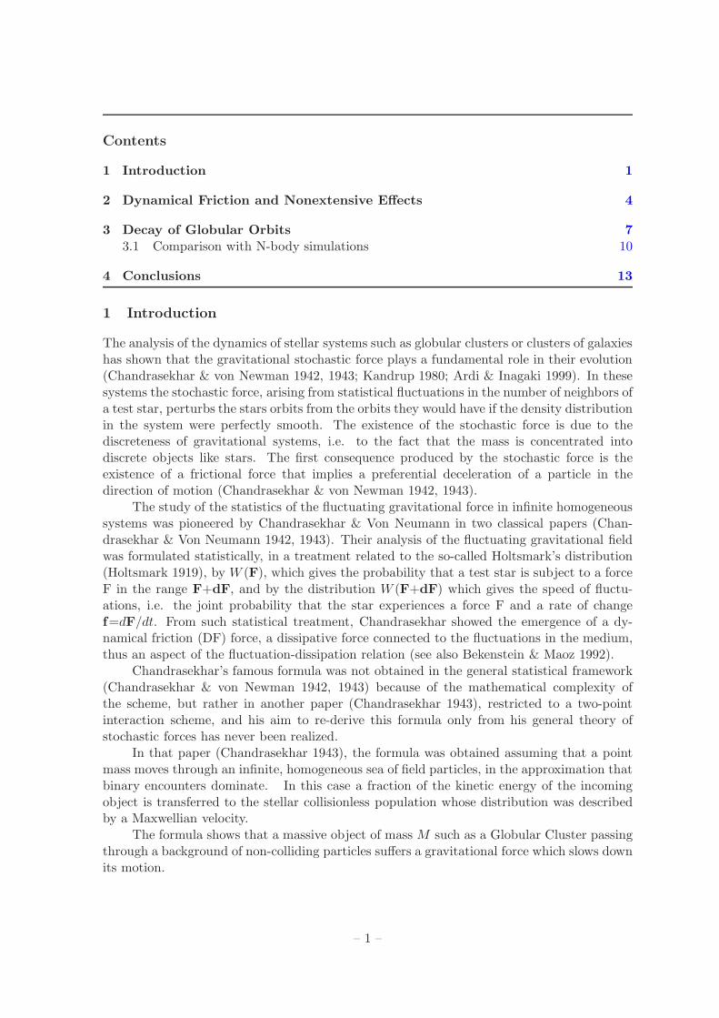
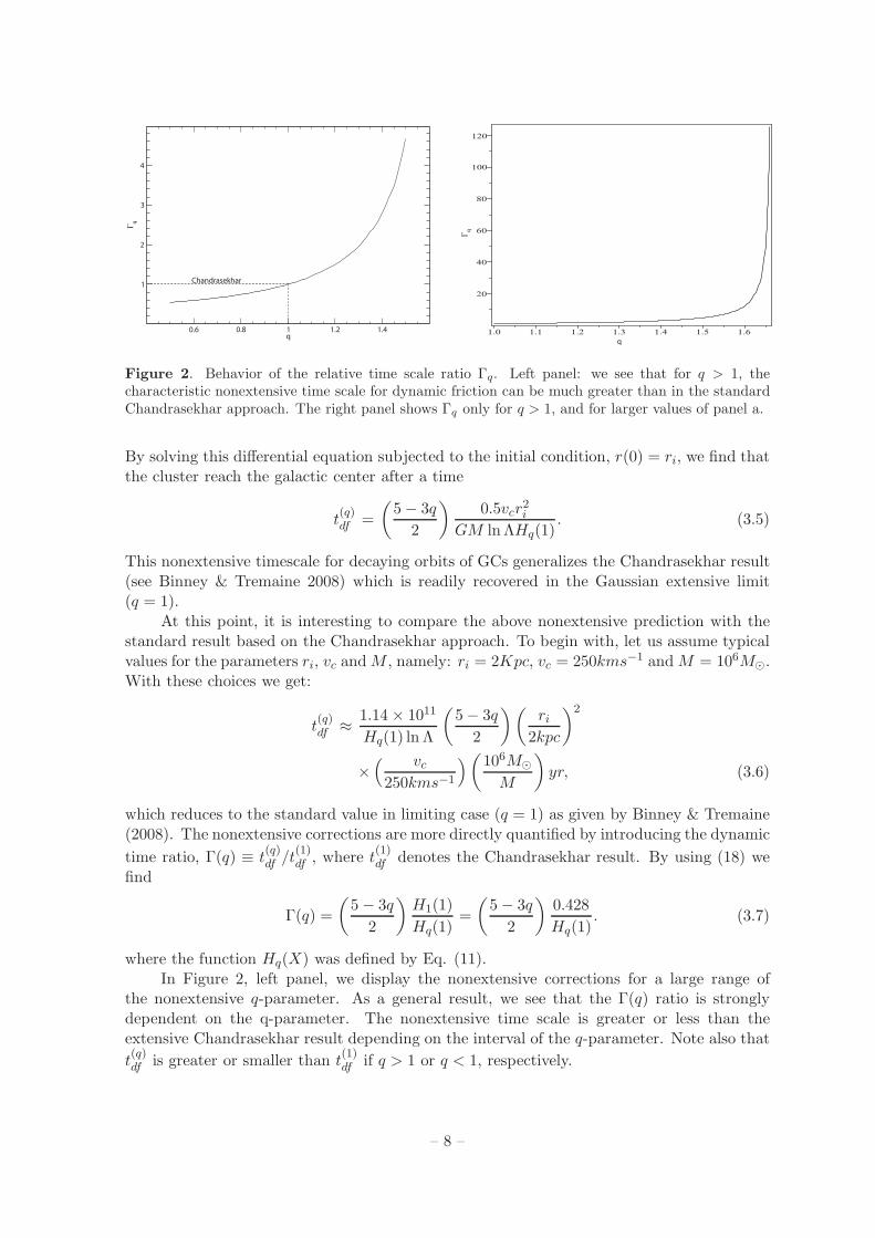
Figure 2. Behavior of the relative time scale ratio Γq. Left panel: we see that for q > 1, thecharacteristic nonextensive time scale for dynamic friction can be much greater than in the standardChandrasekhar approach. The right panel shows Γq only for q > 1, and for larger values of panel a.

By solving this differential equation subjected to the initial condition, r(0) = ri, we find thatthe cluster reach the galactic center after a time

t(q)df =

(

5− 3q

2

)

0.5vcr2i

GM ln ΛHq(1). (3.5)

This nonextensive timescale for decaying orbits of GCs generalizes the Chandrasekhar result(see Binney & Tremaine 2008) which is readily recovered in the Gaussian extensive limit(q = 1).

At this point, it is interesting to compare the above nonextensive prediction with thestandard result based on the Chandrasekhar approach. To begin with, let us assume typicalvalues for the parameters ri, vc andM , namely: ri = 2Kpc, vc = 250kms−1 andM = 106M⊙.With these choices we get:

t(q)df ≈ 1.14 × 1011

Hq(1) ln Λ

(

5− 3q

2

)(

ri2kpc

)2

×( vc250kms−1

)

(

106M⊙

M

)

yr, (3.6)

which reduces to the standard value in limiting case (q = 1) as given by Binney & Tremaine(2008). The nonextensive corrections are more directly quantified by introducing the dynamic

time ratio, Γ(q) ≡ t(q)df /t

(1)df , where t

(1)df denotes the Chandrasekhar result. By using (18) we

find

Γ(q) =

(

5− 3q

2

)

H1(1)

Hq(1)=

(

5− 3q

2

)

0.428

Hq(1). (3.7)

where the function Hq(X) was defined by Eq. (11).In Figure 2, left panel, we display the nonextensive corrections for a large range of

the nonextensive q-parameter. As a general result, we see that the Γ(q) ratio is stronglydependent on the q-parameter. The nonextensive time scale is greater or less than theextensive Chandrasekhar result depending on the interval of the q-parameter. Note also that

t(q)df is greater or smaller than t

(1)df if q > 1 or q < 1, respectively.

– 8 –

0

0.2

0.4

0.6

0.8

1

1.2

0 2 4 6 8 10

r / kp

c

t / Gyr

big coresmall core

small core

cusp

10

This paper

Chandrasekhar

G06

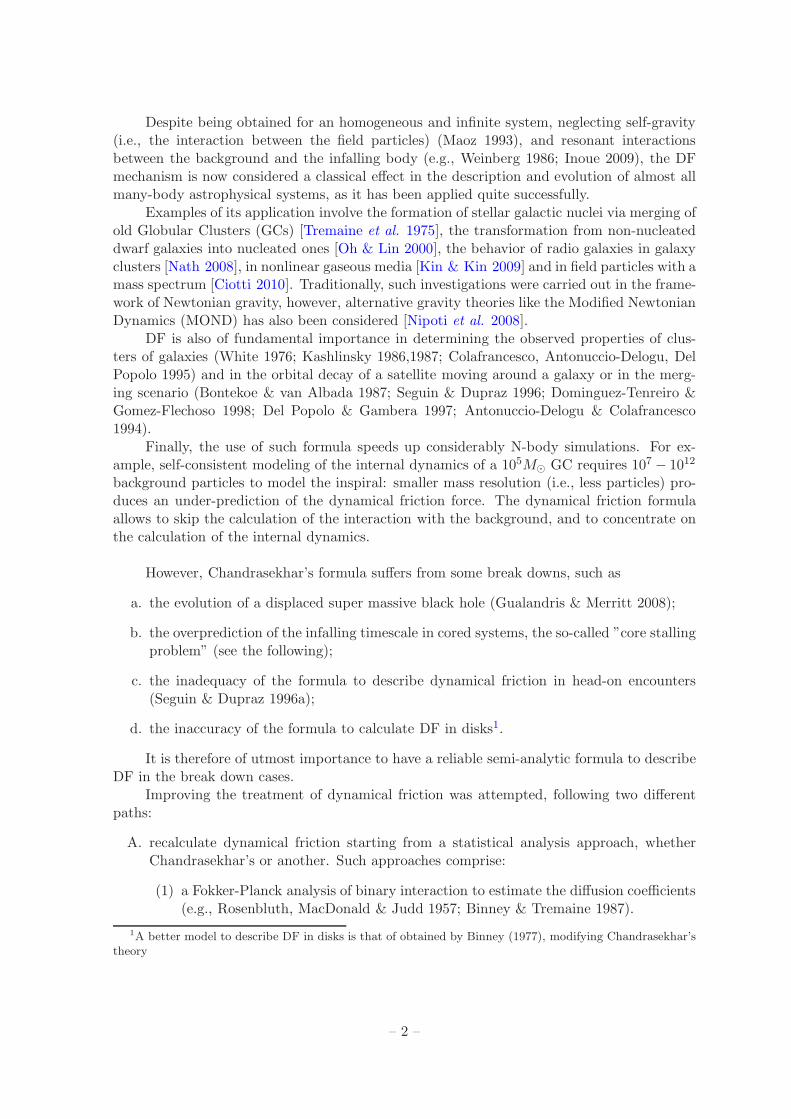
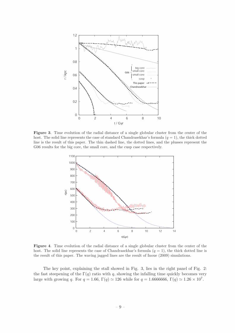
Figure 3. Time evolution of the radial distance of a single globular cluster from the center of thehost. The solid line represents the case of standard Chandrasekhar’s formula (q = 1), the thick dottedline is the result of this paper. The thin dashed line, the dotted lines, and the plusses represent theG06 results for the big core, the small core, and the cusp case respectively.

0

100

200

300

400

500

600

700

800

900

1000

1100

0 2 4 6 8 10 12 14

t(Gyr)

r(p

c)

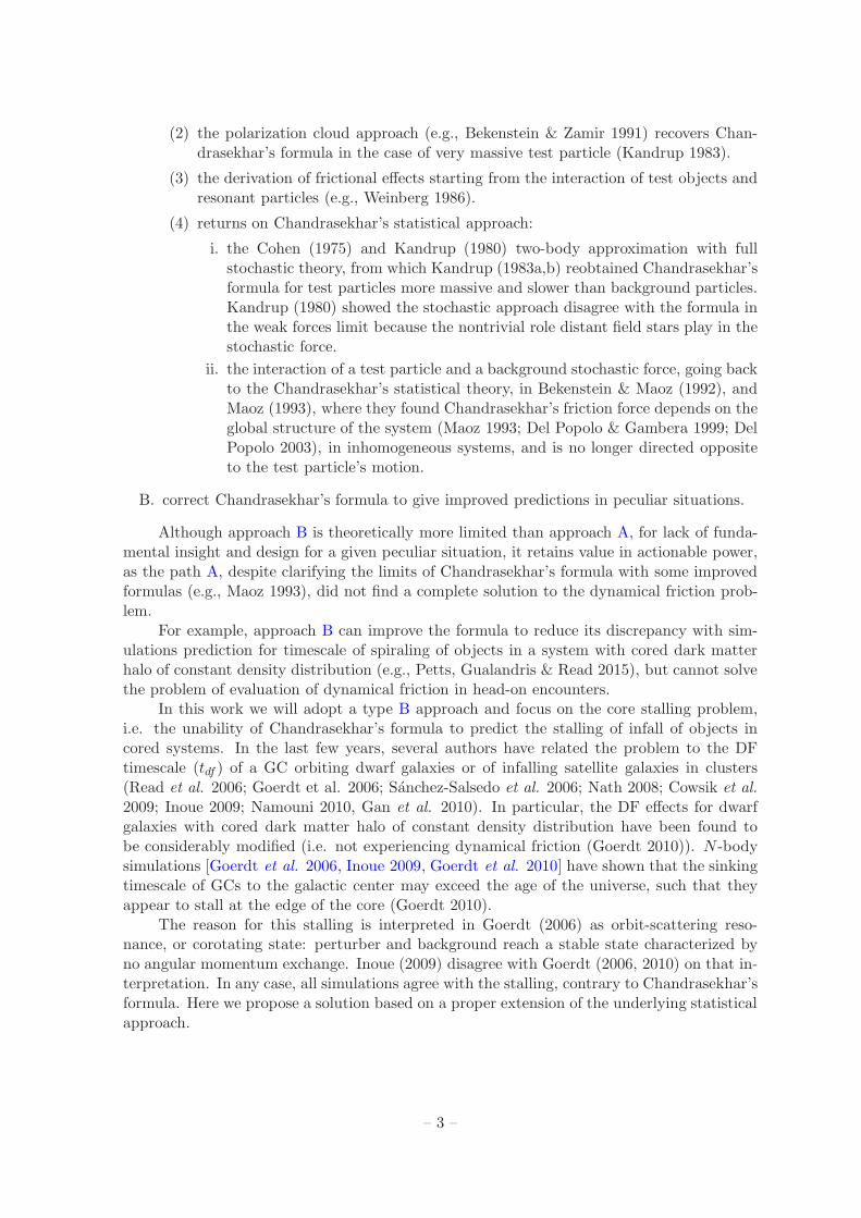
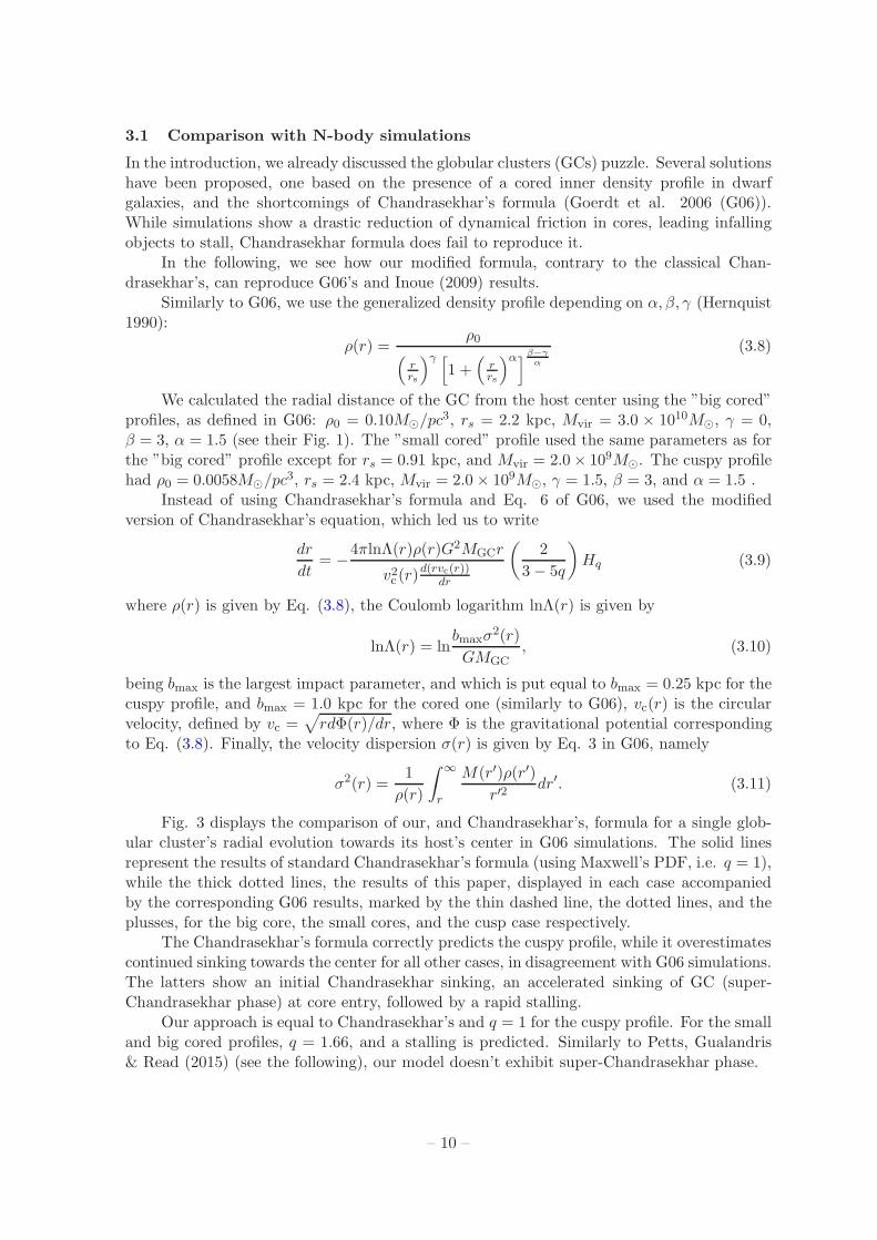
Figure 4. Time evolution of the radial distance of a single globular cluster from the center of thehost. The solid line represents the case of Chandrasekhar’s formula (q = 1), the thick dotted line isthe result of this paper. The waving jagged lines are the result of Inoue (2009) simulations.

The key point, explaining the stall showed in Fig. 3, lies in the right panel of Fig. 2:the fast steepening of the Γ(q) ratio with q, showing the infalling time quickly becomes verylarge with growing q. For q = 1.66, Γ(q) ≃ 126 while for q = 1.6666666, Γ(q) ≃ 1.26 × 107.

– 9 –

3.1 Comparison with N-body simulations

In the introduction, we already discussed the globular clusters (GCs) puzzle. Several solutionshave been proposed, one based on the presence of a cored inner density profile in dwarfgalaxies, and the shortcomings of Chandrasekhar’s formula (Goerdt et al. 2006 (G06)).While simulations show a drastic reduction of dynamical friction in cores, leading infallingobjects to stall, Chandrasekhar formula does fail to reproduce it.

In the following, we see how our modified formula, contrary to the classical Chan-drasekhar’s, can reproduce G06’s and Inoue (2009) results.

Similarly to G06, we use the generalized density profile depending on α, β, γ (Hernquist1990):

ρ(r) =ρ0

(

rrs

)γ [

1 +(

rrs

)α]β−γα

(3.8)

We calculated the radial distance of the GC from the host center using the ”big cored”profiles, as defined in G06: ρ0 = 0.10M⊙/pc

3, rs = 2.2 kpc, Mvir = 3.0 × 1010M⊙, γ = 0,β = 3, α = 1.5 (see their Fig. 1). The ”small cored” profile used the same parameters as forthe ”big cored” profile except for rs = 0.91 kpc, and Mvir = 2.0× 109M⊙. The cuspy profilehad ρ0 = 0.0058M⊙/pc

3, rs = 2.4 kpc, Mvir = 2.0× 109M⊙, γ = 1.5, β = 3, and α = 1.5 .Instead of using Chandrasekhar’s formula and Eq. 6 of G06, we used the modified

version of Chandrasekhar’s equation, which led us to write

dr

dt= −4πlnΛ(r)ρ(r)G2MGCr

v2c (r)d(rvc(r))

dr

(

2

3− 5q

)

Hq (3.9)

where ρ(r) is given by Eq. (3.8), the Coulomb logarithm lnΛ(r) is given by

lnΛ(r) = lnbmaxσ

2(r)

GMGC, (3.10)

being bmax is the largest impact parameter, and which is put equal to bmax = 0.25 kpc for thecuspy profile, and bmax = 1.0 kpc for the cored one (similarly to G06), vc(r) is the circularvelocity, defined by vc =

√

rdΦ(r)/dr, where Φ is the gravitational potential correspondingto Eq. (3.8). Finally, the velocity dispersion σ(r) is given by Eq. 3 in G06, namely

σ2(r) =1

ρ(r)

∫

∞

r

M(r′)ρ(r′)

r′2dr′. (3.11)

Fig. 3 displays the comparison of our, and Chandrasekhar’s, formula for a single glob-ular cluster’s radial evolution towards its host’s center in G06 simulations. The solid linesrepresent the results of standard Chandrasekhar’s formula (using Maxwell’s PDF, i.e. q = 1),while the thick dotted lines, the results of this paper, displayed in each case accompaniedby the corresponding G06 results, marked by the thin dashed line, the dotted lines, and theplusses, for the big core, the small cores, and the cusp case respectively.

The Chandrasekhar’s formula correctly predicts the cuspy profile, while it overestimatescontinued sinking towards the center for all other cases, in disagreement with G06 simulations.The latters show an initial Chandrasekhar sinking, an accelerated sinking of GC (super-Chandrasekhar phase) at core entry, followed by a rapid stalling.

Our approach is equal to Chandrasekhar’s and q = 1 for the cuspy profile. For the smalland big cored profiles, q = 1.66, and a stalling is predicted. Similarly to Petts, Gualandris& Read (2015) (see the following), our model doesn’t exhibit super-Chandrasekhar phase.

– 10 –

Similar comparisons to Inoue (2009) simulations are made in Fig. 4. They followedRead et al (2006), and G06, using the Hernquist’s profile (Eq. 3.8), with ρ0 = 0.10M⊙/pc

3,scale radius rs = 0.91 kpc, an almost constant density within 200-300 pc, and a velocitydispersion obtained from Jeans equation, as in G06. A single GC, on initial circular orbitradius 600 pc or 1 kpc, is followed.

The same line conventions are used to represent this paper’s results and those of Chan-drasekhar’s formula (q = 1). Inoue (2009)’s simulations yield the wavy jagged lines. Asin Fig. 3, Chandrasekhar’s formula does not show any stalling, while our model does, butfails, similarly to Petts, Gualandris & Read (2015), to reproduce the farthest initial GCsuper-Chandrasekhar’s phase.

From these comparisons, we can conclude that the extra parameter q models the effectsof non-locality expected on DF beyond Chandrasekhar’s formula: Petts, Gualandris & Read(2015) obtained core stalling assuming Coulomb logarithm radial dependence, with a null DFfor trajectories with impact parameter smaller or equal to a minimum , bmin, representing ab-sence of particles to scatter off the satellite. They conjectured that the super-Chandrasekharphase could be reproduced by taking into account either super-resonance in the core (e.g.,Goerdt 2010), or faster than satellite host’s stars. The fundamental importance of the latterwas confirmed by Antonini & Merritt (2012) in black hole inspiral with low density back-ground. Their results are further improved using a time dependent distribution functiondirectly extracted from simulations. The principal drawback of such improvement is theneed to run a simulation to obtain the time dependent distribution, before inputting it in theAntonini & Merritt (2012) approach. This issue obviously reduces the predictive power ofthat method, since the simulation already contains the correct description of the motion ofthe infalling body. This problem is not present in Petts, Gualandris & Read (2015) or in thepresently proposed method. However, the result of Antonini & Merritt (2012) is a furtherconfirmation that one limit of Chandrasekhar’s formula lies in its assumption of locality (twobody interactions). The non-locality of beyond Chandrasekhar DF also agrees with resultsfrom approach A: Maoz (1993) (see also Del Popolo & Gambera 1999; Del Popolo 2003)showed DF depends on the global structure of the system, given by a new parameter (q inthe present work), and the DF force direction departs from the opposite to the particle’smotion.

Our present study finds q adopts different values for cuspy and cored profiles to getcorrect r − t behaviour.

At this stage, the question arises whether our semi-analytical model’s stalling capturearises from the extra q, considered as a parameter chosen to reproduce simulations, or asrealistic physics provided by the model. To test this point, we use Eddington’s formulato obtain the phase-space density function (PDF) f(E) corresponding to the sphericallysymmetric density profiles (Eq. 3.8) we used. Comparing the f(E) obtained from the cuspyand cored profiles with our distribution function (Eq. 2.6) can give some hints on this issue,as an agreement between the f(E)s obtained in each case from both methods, Eddington’sor the choice of q in Eq. (2.6) could be considered to imply that our model contains realisticphysics

Such a test is performed in Fig. 5.In the left panel of Fig. 5, the cuspy profile’s PDF from Eddington’s formula is rep-

resented by a solid line, while the dashed line displays the Tsallis’ f(E), obtained from Eq.(2.6) for q = 1. The right panel shows again Eddington’s PDF as the solid line, this time forthe small-cored profile, and that from Tsallis’ (Eq. 2.6) with q = 1.66 as the dashed line.

– 11 –

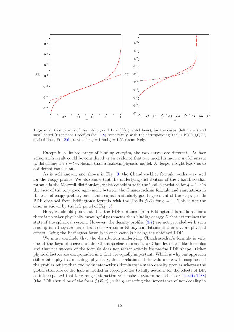
Figure 5. Comparison of the Eddington PDFs (f(E), solid lines), for the cuspy (left panel) andsmall cored (right panel) profiles (eq. 3.8) respectively, with the corresponding Tsallis PDFs (f(E),dashed lines, Eq. 2.6), that is for q = 1 and q = 1.66 respectively.

Except in a limited range of binding energies, the two curves are different. At facevalue, such result could be considered as an evidence that our model is more a useful ansatzto determine the r− t evolution than a realistic physical model. A deeper insight leads us toa different conclusion.

As is well known, and shown in Fig. 3, the Chandrasekhar formula works very wellfor the cuspy profile. We also know that the underlying distribution of the Chandrasekharformula is the Maxwell distribution, which coincides with the Tsallis statistics for q = 1. Onthe base of the very good agreement between the Chandrasekhar formula and simulations inthe case of cuspy profiles, one should expect a similarly good agreement of the cuspy profilePDF obtained from Eddington’s formula with the Tsallis f(E) for q = 1. This is not thecase, as shown by the left panel of Fig. 5!

Here, we should point out that the PDF obtained from Eddington’s formula assumesthere is no other physically meaningful parameter than binding energy E that determines thestate of the spherical system. However, the density profiles (3.8) are not provided with suchassumption: they are issued from observation or Nbody simulations that involve all physicaleffects. Using the Eddington formula in such cases is biasing the obtained PDF.

We must conclude that the distribution underlying Chandrasekhar’s formula is onlyone of the keys of success of the Chandrasekar’s formula, or Chandrasekar’s-like formulasand that the success of the formula does not reflect exactly its precise PDF shape. Otherphysical factors are compounded in it that are equally important. Which is why our approachstill retains physical meaning: physically, the correlations of the values of q with cuspiness ofthe profiles reflect that two body interactions dominate in steep density profiles whereas theglobal structure of the halo is needed in cored profiles to fully account for the effects of DF,as it is expected that long-range interaction will make a system nonextensive [Tsallis 1988](the PDF should be of the form f (E, q) , with q reflecting the importance of non-locality in

– 12 –

the system). We plan to extend that exploration, following Read et al. (2006), finding theinfall dependence on density profile inner slope and satellite mass. Finally, a future studyshould explore if a q(r) dependence can reproduce the super-Chandrasekhar phase.

We want now to recall that the GCs decay time puzzle is strictly connected to anotherfundamental problem of the ΛCDM model, namely the nature of the inner density profiles ofdwarf galaxies, the so called cusp/core problem (Flores & Primack 1994; Moore 1994). Thefact that the MW dSphs are not nucleated, and only around 30% of those in clusters are,may imply that the inner density profiles of the MW dSphs are cored. Kleyna et al. (2003)studying the stellar number density in the Ursa Minor dSph (Umi dSph), concluded thatthe second peak in the stellar number density is unreconcilable with a cuspy profile. Morerecently many authors have studied the problem of the inner structure of the MW dSphs,since this could give information on the nature of DM. As discussed by several authors (e.g.,Penarrubia et al. 2012) cored inner profiles in low mass dSphs would increase the knowntension between some of the small scale problems of the ΛCDM. Unfortunately, controversialevidences have been presented (e.g., Jardel et al. 2013; Amorisco & Evans 2012; Jardel et al.2013) to date due to the difficulty to distinguish cusps from cores (e.g., Strigari et al. 2014)and this leaves the inner structure of dSph galaxies as a still open debate.

4 Conclusions

We have derived the q-dynamic friction force for a point mass moving through a homogeneousbackground in the context of the nonextensive kinetic theory. Simple and analytical formswere obtained, and, as should be expected, they smoothly reduce to the standard Chan-drasekhar results in the extensive limiting case (q = 1). However, for q 6= 1 a large varietyof qualitatively different behaviors are predicted when the free parameter q is continuouslyvaried (see Figs. 1 e 2). As an application, we have discussed

a. the dynamical timescale for a globular cluster collapsing to the center of a massive darkmatter halo described by an isothermal sphere,

b. we showed that the evolution of the radial distance in the case of the ”small” and ”bigcored” profiles studied by Goerdt et al (2006) may be reobtained in the case q = 1.66,and

c. we confronted the q-modified Chandrasekhar formula with two sets of Nbody simula-tions that reveal how successful the model is at reproducing the core stalling. Howeverit reveals that a super-Chandrasekhar phase is yet to be properly modeled.

The results presented here suggest that the problem related to the large timescale shownby numerical N -body simulations and semi-analytical models may naturally be solved (withno ad hoc mechanism) by taking a proper q-nonextensive distribution with parameter greaterthan unity. Applications to other density profiles like the lowered nonextensive halos distri-bution (Silva, de Souza & Lima 2009; Cardone, Leubner & Del Popolo 2011) and a detailedcomparison with semi-analytical models will be discussed in a forthcoming communication.

Acknowledgments: JMS is supported by FAPESP Agency and JASL by FAPESP andCNPq (Brazilian Research Agencies). The work of M.Le D. has been supported by PNPD/CAPES20132029.M.Le D. also wishes to acknowledge IFT/UNESP. ADP wishes to thank Dian-Yong Chenfrom Laznhou IMP-CAS.

– 13 –

References

[Abramowitz & Stegun 1972] Abramowitz M. & Stegun I.A. 1972, Handbook of MathematicalFunctions, Dover, NY

[Am] Amorisco N. C., Evans N. W., 2012, MNRAS, 419, 184

[An] Antonini F. and Merritt D., , 2012, Ap.J., 745, 83

[A] Antonuccio-Delogu V., Colafrancesco S., 1994, ApJ, 427, 72

[Ardi] Ardi, E., & Inagaki, S., 1999 IAUS 186, 408

[beZ] Bekenstein, J. D., Zamir, R., 1990, ApJ 359, 427

[bek] J. D. Bekenstein, E. Maoz, 1992, ApJ 390, 79

[bin] Binney, J., 1977, MNRAS 181, 735

[Binney & Tremaine 2008] Binney J. & Tremaine S. 2008, Galactic Dynamics. Princeton Univ.Press, Princeton, NJ

[B] Bontekoe, T. R., van Albada, T. S., 1987, MNRAS, 224, 349

[Boylan-Kolchin et al. 2008] Boylan-Kolchin M. et al. 2008, MNRAS 383, 93

[12] Cardone V. F., Leubner, M. P. & Del Popolo A. 2011, MNRAS 414, 2265

[Chandrasekhar & von Newman 1942] Chandrasekhar, S., von Neumann, J., 1942, Ap.J., 95,489

[Chandrasekhar & von Newman 1943] Chandrasekhar S., von Neumann J., 1943, ApJ, 97, 1

[Chandrasekhar 1943] Chandrasekhar S. 1943, ApJ 97, 255

[Ciotti 2010] Ciotti L. 2010, AIP Conference Proceedings 1242, 117

[Co] Colafrancesco, S., Antonuccio-Delogu, V., Del Popolo, A., 1995, ApJ 455, 32

[Cowsik et al. 2009] Cowsik R. et al. 2009, ApJ 699, 1389

[DPG97] Del Popolo A., Gambera M, 1997A&A...321..691D

[D] Del Popolo, A., & Gambera, M., 1999 A&A 342, 34

[Del] Del Popolo, A., 2003A&A 406, 1

[D] Dominguez-Tenreiro, R., Gomez-Flechoso, M. A., 1998, MNRAS 294, 465

[Fellhauer 2008] Fellhauer M. 2008, Lect. Notes Phys. 760, 171

[F] Flores R. A., Primack J. R., 1994, ApJL, 427, L1

[Gan et al. 2010] Gan J-L. et al. 2010, Res. Astron. Astrophys. 10 1242

[Gel-Mann & Tsallis 2004] Gell-Mann, M., & Tsallis, C. (ed.) 2004, Nonextensive Entropy:Interdisciplinary Applications (New York: Oxford Univ. Press)

[Goerdt et al. 2006] Goerdt T. et al. 2006, MNRAS 368, 1073

[Goerdt et al. 2010] Goerdt T. , Moore B., Read J. I., and Stadel J., 2010, ApJ, 725, 1707

[Gruess et al. 2009] Grues X. M., Lou Y.-K. & Duschl W. J. 2009, MNRAS 400, L52

[Hansen et al. 2005] Hansen S. H. et al. 2005, New Astron. 10, 379

[H19] Holtsmark P.J., 1919, Phys. Z., 20, 162

[Inoue 2009] Inoue S. 2009, MNRAS 397, 709

[j] Jardel J. R., Gebhardt K., Fabricius M. H., Drory N., Williams M. J., 2013, ApJ, 763, 91

[Kandrup1980] Kandrup H.E., 1980a, Phys. Rep., 63, n. 1, 1

– 14 –

[K] Kashlinsky A., 1986, ApJ, 306, 374

[K1] Kashlinsky A., 1987, ApJ, 312, 497

[Kin & Kin 2009] Kin H. & Kin W.-T. 2009, ApJ 703, 1278

[Kl] Kleyna J. T., Wilkinson M. I., Gilmore G., Evans N. W., 2003, ApJ 588, L21 erratum, ibid.2003, 589, L59

[Kronberger et al. 2006] Kronberger T. et al. 2006, A&A 453, 21

[Lapenta 2007] Lapenta, G., Markidis, S., Marocchino, A., & Kaniadakis, G. 2007, ApJ, 666, 949

[Lavagno et al. 1998] Lavagno A. et al. 1998, Astrop. Lett. Comm. 35, 449

[Leubner 2005] Leubner M. P. 2005, ApJ 632, L1

[Lima & de Souza 2005] Lima J. A. S. & de Souza R. E. 2005, Physica A 350, 303,astro-ph/0406404

[44] Lima J. A. S., Plastino A. R. & Silva R. 2001, Phys. Rev. Lett. 86, 2938, cond-mat/0101030

[46] Lima J. A. S., Silva R. & Santos J. 2000, Phys. Rev. E 61, 3260,

[46] Lima J. A. S., Silva R. & Santos 2002, A&A 396, 309, astro-ph/0109474

[m] Maoz E., 1993, MNRAS 263, 75

[m] Moore B., 1994, Nature, 370, 629

[Namouni 2010] Namouni F. 2010, MNRAS 401, 319

[Nath 2008] Nath B. B. 2008, MNRAS 387, L50

[Nipoti et al. 2008] Nipoti C et al. 2008, MNRAS 386, 2194-2198

[Oh & Lin 2000] Oh K. S. & Lin D. N. 2000, ApJ 543, 620.

[pen] Penarrubia J., Pontzen A.,Walker M. G., Koposov S. E., 2012,ApJL, 759,L42

[petts] J. A. Petts, A. Gualandris, J. I. Read, arXiv:1509.07871v1

[Read et al. 2006] Read J. I. et al. 2006, MNRAS 373, 1451

[Rosenbluth et al. 1957] Rosenbluth M. N., MacDonald W. M., Juss, D. L., 1957, Phys. Rev. 101, 7

[Sanchez-Salcedo et al. 2006] Sanchez-Salcedo F. J. et al. 2006, MNRAS 370, 1829

[S] Seguin, P., Dupraz, C., 1996, A & A, 310, 757

[59] Silva J. M., R. E. de Souza & J. A. S. Lima 2009, [arXiv:0903.0423].

[60] Silva R., Plastino A. R. & Lima J. A. S. 1998, Phys. Lett. A 249, 401

[Silva et al. 2009] Silva J. M., R. E. de Souza & J. A. S. Lima 2009, [arXiv:0903.0423]

[S] Strauss M.A., Willick J.A., 1995, Phys. Rept., 261, 271

[St] Strigari L. E., Frenk C. S., White S. D. M., 2014, arXiv:1406.6079

[Taruya & Sakagami 2002] Taruya A. & Sakagami M. 2002, Physica A 307, 185

[Tremaine et al. 1975] Tremaine S. et al. 1975, ApJ 196, 407

[Tsallis 1988] Tsallis C. 1988, J. Stat. Phys. 52, 479

[Tsallis 2009] Tsallis C., Introduction to Nonextensive Statistical Mechanics: Approaching a

Complex World, Springer (2009)

[w] White, S. D. M., 1976, MNRAS, 174, 19

[wein] Weinberg, M. D., 1986, ApJ 300, 93

– 15 –