i

Chalmers Thesis Template Master’s Thesis in Evaluation and Implementation of Error Control Coding Schemes in Industrial Wireless Sensor Networks

YONAS HAGOS YITBAREK Department of Signals and Systems

Division of Communication Engineering

CHALMERS UNIVERSITY OF TECHNOLOGY

Göteborg, Sweden, 2014

Master’s Thesis EX013/2014

ii

Performed at: ABB Corperate Research, Västerås, Sweden.

Supervisors at ABB:

1. Mikael Gidlund (mikael.gidlund@se.abb.com)

2. Johan Åkerberg (johan.akerberg@se.abb.com)

3. Kan Yu (kan.yu@mdh.se)

Examiner:

Alexandre Graell I Amat (alexandre.graell@chalmers.se)

Supervisor at Chalmers:

Naga Vishnukanth Irukulapati (vnaga@chalmers.se)

© YONAS HAGOS YITBAREK, 2014

Diploma work no xx/2014

Department of Signals and Systems

Division of Communication Engineering

Chalmers University of Technology

SE-412 96 Gothenburg, Sweden

iii

iv

v

Abstract

In process automation, Industrial Wireless Sensor Networks (IWSNs) plays a tremendous

role due to great number of advantages such as cable cost reduction, convenient installation, flexible deployment and maintenance. IWSNs have stringent requirements on reliability and

real time performances. However, transmission of wireless signals over harsh industrial

wireless channel is vulnerable to noise and interference which causes high risk of packet transmission failure. Consequently, packet loss in industrial automation leads to delay of

process or control data which may terminate industrial applications and finally results in

huge economic loss and safety problems. IWSNs commonly use error correcting mechanisms to increase communication reliability and improve real time performances.

On a Media Access Control (MAC) layer, the existing protocol in IWSNs employs an

Automatic Repeat Request mechanism to improve reliable packet delivery at the cost of real time performance. Forward Error Correction (FEC) coding scheme on a MAC layer is

proposed to improve reliability and reduce latency by decreasing the number of packet

retransmissions. In this thesis, several FEC coding schemes are studied and implemented in typical IWSN chip to evaluate its execution time and ensure that the strict acknowledgement

timing requirement of the standard is preserved. In addition to that, the memory

consumption of FEC schemes is evaluated as the embedded devices of IWSNs are memory constrained. The result of our evaluation shows that certain FEC coding schemes, such as RS

code, are suitable to be implemented in IWSN node while the state of the art FEC codes, such

as Turbo and LDPC codes, fail due to huge memory consumption and long execution time of

their encoding and decoding algorithms.

vi

Acknowledgement

First, I would like to express my sincere gratitude and appreciation to my Supervisors Dr.

Mikael Gidlund (ABB Corporate Research) and Dr. Johan Åkerberg (ABB Corporate Research) for the golden opportunity they have given me and believing in me. Their

continuous follow up, guidance and support throughout the thesis work was inspiring and

very helpful. I would like also to thank Yu Kan for his advice, discussions and help during the work.

I would also like to express my appreciation and thanks to my examiner Dr. Alexandre

Graell I Amat and my supervisor Naga Vishnukanth Irukulapati at Chalmers University of Technology for their useful comments, remarks and supervision.

My special gratitude goes to Swedish International Development Cooperation Agency

(SIDA) for offering me a scholarship to study my master’s programme.

Furthermore, I want to express my special thanks to all friends at ABB Corporate Research

for all the experience sharing, discussion, support, moments of laughter and fun.

Personally, I would like to thank my family for their overwhelming love, encouragement and support they give me at every step of my life.

vii

Table of Contents

Abstract v

Acknowledgement vi

Table of Contents vii

List of Figures ix

List of Tables x

List of Acronyms xi

1 Introduction……………………………………………………………………………………….1

1.1 Research Problems…………………………………………………………………………..1

1.2 Approach to Problems………………………………………………………………………2

1.3 Thesis Contributions………………………………………………………………………...2

1.4 Related Work………………………………………………………………………………...3

1.5 Thesis Outline………………………………………………………………………………..4

2 Industrial Wireless Sensor Networks..…………………………………………………………5

2.1 IWSN Structure……………………………………………………………………………....5

2.2 IWSN Standards……………………………………………………………………………...7

2.2.1 IEEE 802.15.4…………………………………………………………………………...7

2.2.2 IEEE 802.15.4-based Standards……………………………………………………...11

2.3 Industrial Wireless Channel Conditions…………………………………………………11

3 Preliminaries on Error Control Coding and ARM Platform.……………………………….14

3.1 Forward Error Correction Codes…………………………………………………………14

3.1.1 Linear Block Codes…………………………………………………………………...14

3.1.1.1 General Properties of Linear Block Codes……………………………...16

3.1.1.2 Repetition Code…………………………………………………………...20

3.1.1.3 Hamming Code…………………………………………………………...21

3.1.1.4 Classic Cyclic Code………………………………………………………22

3.1.1.5 BCH Code………………………………………………………………….27

3.1.1.6 RS Code…………………………………………………………………... 30

3.1.2 LDPC and Turbo Codes……………………………………………………………..31

3.1.2.1 LDPC Codes………………………………………………………………31

3.1.2.2 Turbo Code………………………………………………………………..32

3.2 Introduction to ARM Platform…...……………………………………………………….35

4 Implementation and Performance Evaluation……………………………………………….38

viii

4.1 Applying FEC in IWSNs…………………………………………………………………..38

4.1.1 FEC in MAC Layer…………………………………………………………………...38

4.1.2 Timing Requirement…………………………………………………………………39

4.1.3 Memory Resource…………………………………………………………………….39

4.2 Complexity Algorithms……………………………………………………………………39

4.2.1 Time Complexity……………………………………………………………………..40

4.3 Measurement Setup………………………………………………………………………..40

4.3.1 Implementation Tools and Settings……………………………………………….40

4.3.2 Implementation Sources……………………………………………………………40

4.3.3 Methods for Measurement………………………………………………………...41

4.3.3.1 Memory …………………………………………………………………….41

4.3.3.2 Processing Time……………………………………………………………42

4.4 Performance Evaluation…………………………………………………………………...43

4.4.1 Evaluation Result of Block Codes…………………………………………………..44

4.4.2 Evaluation Result of LDPC, Turbo and Block Codes……………………………..60

5 Conclusions and Future works………………………………………………………………...72

5.1 Summary and Conclusions………………………………………………………………..72

5.2 Future Works……………………………………………………………………………….72

6 References………………………………………………………………………………………..73

7 Appendix ……………………………………………………………………………………......78

ix

List of Figures 1. An industrial wireless sensor network structure 6

2. Data transmission with acknowledgement [10] 8

3. IEEE 802.15.4 Data Frame [61] 10

4. Power Plant [10] 12

5. The measured RSSI transmitted data in scenario 1 [10] 13

6. The measured RSSI transmitted data in scenario 2 [10] 13

7. Shift register encoder 23

8. Meggitt decoder for cyclic code 24

9. BCH decoder with 2mGF arithmetic operations [5] 27

10. Linear Feedback Shift Register (LFSR) 29

11. Reed Solomon (RS) decoder with 2mGF arithmetic operations 31

12. Turbo code system [60] 33

13. Turbo encoder 33

14. Recursive systematic convolutional code 34

15. Turbo decoder [60] 34

16. STM32W108 application board 37

17. IEEE 802.15.4 data frame structure [10] 38

18. Voltage of LEDs 42

19. Footprint of block codes using none optimization 47

20. Footprint of block codes using high size optimization 47

21. Footprint of block codes using high speed optimization 48

22. Footprint of block codes using high balance optimization 48

23. FEC performance relative to capacity bound 61

24. Footprint of FEC using none optimization 63

25. Footprint of FEC using high size optimization 64

26. Footprint of FEC using high speed optimization 64

27. Footprint of FEC using high balance optimization 65

x

List of Tables

1. Frequency bands and data rate of IEEE 802.15.4 [16] 9

2. Definitions of MacAckWaitDuration parameters and values 10

3. Definition of error probabilities 18

4. Syndrome table of meggitt decoder for cyclic (15, 7) code 26

5. Code rates and error correcting capability of BCH and RS codes 44

6. Execution time of block codes with none optimization 44

7. Execution time of block codes with high speed optimization 45

8. Execution time of block codes with high size optimization 45

9. Execution time of block codes with high balance optimization 46

10. Time complexity of block coding algorithms 58

11. Execution time of FEC with none optimization 61

12. Execution time of FEC with high speed optimization 62

13. Execution time of FEC with high size optimization 62

14. Execution time of FEC with high balance optimization 63

xi

List of Acronyms

ACK Acknowledgement

ADC Analog to Digital Converter

ARQ Automatic Repeat reQuest

ARM Advanced RISC Machine

ASK Amplitude Shift Keying

BER Bit Error Rate

BPSK Binary Phase Shift Keying

BCH Bose-Chaudhuri-Hocquengham

BMA Berlekamp Massey Algorithm

CIWA Chinese Industrial Wireless Alliance

CPU Central Processing Unit

CSMA-CA Carrier Sense Multiple Access with Collision Avoidance

DSSS Direct Sequence Spread Spectrum

EA Euclidean Algorithm

ECC Error Control Coding

FCS Frame Check Sequence

FEC Forward Error Control

GTS Guaranteed Time Slot

HCF HART Communication Foundation

IAR Ingenjörsfirma Anders Rundgren

ISA International Society Automation

ISM Industrial, Scientific and Medical

IWSN Industrial Wireless Sensor Network

LAN Local Area Network

LDPC Low Density Parity Check

LFSR Linear Feedback Shift Register

LQI Link Quality Indicator

MAC Media Access Control

MCU Micro Controller Unit

MFR Mac Footer

MHR MAC Header

NLOS Non Line Of Sight

O-QPSK Orthogonal Quadrature Phase Shift Keying

PAN Personal Area Network

xii

PHY Physical

PSSS Parallel Sequence Spread Spectrum

RF Radio Frequency

RS Reed Solomon

RISC Reduced Instruction Set Computer

RAM Random Access Memory

ROM Read Only Memory

RO Read Only

RW Read Write

SPI Serial Peripheral Interface

SR Shift Register

UART Universal Asynchronous Receiver/Transmitter

WIA-PA Wireless Networks for Industrial Automation Process

Automation

WLAN Wide Local Area Network

WPAN Wireless Personal Area Network

WSN Wireless Sensor Network

xiii

1

Chapter 1

Introduction

Industrial automation is one category of automation widely used in industries to provide

automated solutions. It consists of hardwares such as microcontroller, fieldbus, sensors and

actuators, and softwares such as control and communication software. It is a technology that

integrates the hardware and software solutions to automate repetitive manual tasks in order

to have better productivity quality and expanded production. It also helps to eliminate

human error which in turn reduces cost and increase quality.

Reliability and real time performance of communication technologies are critical concepts

that should be given more emphasis in automation applications. Reliability is a metric that is

integrated with industrial monitoring and control systems. In communication systems, signal

is degraded due to interference and random noise that can potentially bring a complete

system malfunction, huge economic loss and safety problems in industries. Consequently,

different techniques should be used to ensure a reliable wireless communication system. Real

time performance is also very critical in industrial automation which refers to robust and low

latency signal delivery within the communication systems. Therefore, reliability and real

time capability are essential metrics that should be given more attention in industrial

automations.

In automotive industries, the medium of communication among different devices was

traditionally wired, such as twisted pair cables, coaxial cables and fiber optics to mention

few. Wired communication has a reliable and real time performance in which interference

and network congestion are reduced. Currently, wired communication is not a good choice

in industrial automation due to its cost, deployment complexity and maintenance

constraints. As wireless technologies emerged, dealing with radio became interesting topic.

Flexibility, low cost, robustness, low maintenance, monitoring and control are attractive

benefits of wireless technologies which makes it invaluable option in industrial automation.

Nowadays, Industrial Wireless Sensor Networks (IWSNs) are most widely using wireless

technologies. However, industrial wireless channel has a very huge impact in wireless

communication systems. In wireless communications, signals are easily deteriorated due to

shadowing, interference, path loss and multipath fading and lead to packet loss or delay of

control or process data, and system disturbance that results in termination of industrial

applications which finally may result in huge economic loss and safety problems. Therefore,

reliability and real time performance in IWSNs are extremely important requirements to deal

with in industrial automation applications.

1.1 Research Problem

Currently, communication reliability and real time performance are very critical issues that

should be given more emphasis in IWSNs. The industrial wireless channel is very harsh and

degrades the transmitted signal due to interference, noise and multipath fading. Therefore, it

2

is very difficult situation to guarantee high reliable and low latency communications for

IWSNs in such a harsh industrial environment.

The existing IWSNs employ the IEEE 802.15.4 standard. It applies Automatic Repeat Request

(ARQ) mechanism on a media Access Control (MAC) layer for error correction purpose to

increase the link reliability at the expense of real time performance. Because of the harsh

industrial channel, the failure in packet reception initiates the process of retransmission. The

maximum number of retransmission when a sender failed to transmit successfully is allowed

by the standard. For hundreds of sensor nodes that can operate in a harsh industrial channel,

lots of packet retransmissions are required due to the channel behavior. The excessive

number of retransmission brings communication latency to industrial applications. It also

leads to exhaust the limited bandwidth resource due to many number of nodes trying to

retransmit packets at the same time. The excessive retransmission does not only bring

communication latency to industrial applications but also results in network congestion [11].

Consequently, industrial application process may halt and results in serious economic loss

and safety problems.

Therefore, more robust and advance solution for error correction mechanism on a MAC layer

should be proposed that can address the above problems and improves both reliability and

real time performance in IWSNs. Another problem is that, the application specific embedded

devices in IWSNs has less memory compare to desktop computers and the error correction

mechanism should be carefully chosen by taking this constraint into consideration.

1.2 Approach to Problem

In order to choose the most appropriate error correction mechanism on a MAC layer that

improves reliability and real time performance in IWSNs, the strict timing requirement of the

IEEE 802.15.4-based IWSN standard and the memory constraint of embedded devices should

be fulfilled. Forward Error Correction (FEC) code is one of the appropriate approaches

proposed to be implemented in typical IWSN nodes. In FEC code, redundancy bits are

imposed on the transmitted data in order to recover the bits in error caused by the harsh

wireless channel. The FEC code is the suitable approach to apply due to its capability to

reduce bit error rates and results in decreasing the number of packet retransmission.

However, the processing time of FEC code should be within the timing requirement of IEEE

802.15.4 standard and have reasonable memory footprint, which is the amount of memory

used by a program while running. Therefore, different FEC coding schemes are studied and

proposed for further evaluation in terms of processing time and memory consumption. The

software implementations of all the coding schemes are written in C programming language

and an existing IWSN-chip is used as our platform. Finally, the performance of all FEC

candidates is evaluated and followed by our discussion and analysis.

1.3 Thesis Contribution

The main contributions of this thesis project are

1. A comprehensive survey of most commonly used Error Control Coding (ECC)

schemes.

3

2. Evaluation of different FEC candidate algorithms using software implementation and

comparison of their performances with each other interms of execution time and

memory consumption.

The FEC coding algorithms on a MAC layer suitable for IEEE 802.15.4-based IWSN standard

are proposed. It is shown that some of the algorithms can fit into the IWSN standard to

improve reliability and real time performance without violating the standard format,

requirement and any connection with chip manufactures.

1.4 Related Work

In this section, previous research works related to our thesis are presented. As it was

mentioned earlier, applying FEC mechanism on a MAC layer is proposed to improve

reliability and real time performance in IWSNs.

Significantly, many researches have been carried out regarding performance evaluation of

FEC coding in Wireless Sensor Networks (WSNs). Many researches are performed on FEC

for WSNs emphasis on energy efficiency of FEC coding schemes and FEC related methods.

In [21], even though the use of ECC decreases the transmission power, the complex decoder

needs processing energy, and therefore, exploring this trade off they found that applying

ECC is more power efficient system and analog decoder implementation performed better

than its digital counterpart. Authors in [22] examined the impact of error control

mechanisms on packet size optimization and energy efficiency, and they identify that FEC

scheme is found to be more energy efficient than retransmission mechanism although it

introduces redundancy and requires additional energy for encoding/decoding process.

Furthermore, it is found that Bose-Chaudhuri-Hocquengham (BCH) codes outperformed

convolutional code by 15% in terms of energy efficiency [22]. Authors in [23] also evaluated

FEC and infinite ARQ mechanism and compared in terms of energy efficiency. In this regard,

FEC scheme is found to perform better than the infinite ARQ scheme. Due to the

introduction of redundancy bits and encoding/decoding algorithms energy consumptions,

the performance of FEC schemes in terms of energy efficiency became more interesting.

Therefore, in [24], authors found out that LDPC codes are more energy efficient compared to

BCH codes and convolutional codes. Authors in [25] identified that, after analyzing the

performance of different FEC codes, BCH, Reed-Solomon (RS) and convolutional codes in

terms of their BER and power consumption on different platform, binary-BCH codes with

ASIC implementation are more suitable for WSNs. The authors in [26] analyzed the classical

FEC and carried out an experiment that revealed FEC codes decrease BER in WSN and

concluded that FEC algorithms empower WSNs which increase the area coverage of the

nodes maintaining the same Signal to Noise Ratio (SNR). As a result, a few numbers of nodes

tend to cover the given area which decreases the network costs. However, the

encoding/decoding time of the algorithm seems to violate the standard requirement. The

development of Physical layer – Media Access Control layer (PHY-MAC) cross layer

approach is proposed in [27] to reduce the energy consumption through the use of FEC

coding. This coding mechanism reduces retransmissions at the MAC layer, therefore, the

nodes in the network go to sleep mode quickly which in turn saves energy.

4

Researches on adaptive FEC mechanism have also been done for various WSNs applications.

Authors in [28] showed that adaptive FEC performs better than conventional FEC

mechanisms in terms of transmission reliability and it can also reduce energy consumption

and latency. The hybrid-ARQ-adaptive-FEC scheme in [29] is considered based on BCH

codes and channel state information and is shown that there is significant improvement in

performance compare to ARQ mechanism in terms of latency, packet loss and energy

expenditure. In [30], an adaptive FEC erasure coding scheme is used based on multipath

routing protocol and it is shown that reliable packet delivery has been improved in WSNs

while reducing the network traffic. A hybrid-feedback mechanism is proposed in [31] where

the sink sends ACK packets to the source and expected energy cost of data transmission is

derived based on the ACK. In [31], it is shown that the hybrid mechanism improves the

energy efficiency of multipath data transmission compared to the FEC-based mechanism

under the same reliability constraint.

A combination of FEC coding and routing mechanisms is another trend in FEC related

works. A lightweight FEC coding algorithm which is XOR-based combined with a fault

tolerant routing scheme is proposed in [32]. The FEC coding algorithm is based on multipath

in which a data is fragmentized in to a number of packets and sent over multiple paths. The

routing scheme makes the nodes aware of the failed path in order to choose the optimal path

for routing. Authors in [33] showed that the efficient combinations of information

redundancy like retransmission, FEC coding and alternative routing schemes effectively

improve the reliability.

1.5 Thesis Outline

This report has the following structure.

In chapter 2, an introduction to the concept of IWSNs, IEEE 802.15.4 standard and short

explanation about the other IEEE 802.15.4-based standards are presented.

In chapter 3, the preliminary section that presents the basic background of FEC codes and the

introduction of our benchmarking platform are given.

In chapter 4, the implementation and evaluation of FEC in IWSNs, the basic requirements of

the IWSN standard and constraints of the embedded devices are presented. It also presents

the complexity algorithm of the candidates, the source of the software implementation of the

FEC coding algorithms, the measures and methods used for our evaluations. Finally, the

evaluation results of our algorithms are presented.

In chapter 5, the conclusions and future works are presented.

5

Chapter 2

Industrial wireless sensor networks

In the world of competitive industries, many companies encounter growing demand to

improve process efficiencies, obey the environmental regulations and meet the corporate

financial objectives. The rapid growth of industrial systems, dynamic industrial

manufacturing markets, and intelligent and low cost industrial automation systems are

highly required to improve the productivity and efficiency of the system. Traditionally, the

medium for industrial communication in automation systems are wired. However, the wired

systems require high cost of communication cable installation and maintenance, less flexible

system, and thus, they are not widely employed in industrial plants due to high cost and

inconvenient deployment process. Therefore, cost effective and flexible wireless automation

systems are the urgent requirements in industrial automation systems.

With the recent advances in WSNs, the realization of low cost embedded industrial

automation systems have become feasible. WSN is built of spatially distributed sensor nodes

and gateways. The sensor nodes are installed on industrial equipment to monitor the

parameters critical to each equipment’s based on a combination of measurements such as

vibration, pressure, temperature and power quality which are transmitted through the

wireless channel to sink node that analyzes the data from each sensors. The IWSNs have

several benefits over traditional WSNs (wired) in self organization, rapid deployment,

flexibility and inherent intelligent processing capability. In traditional WSNs, power

consumption is more critical than latency and reliability since a frequent change of batteries

is challenging.

The requirements for IWSNs are different compare to traditional WSNs. Centralized in case

of management is more necessary than self-organization. The operators in center should

have all information and be aware of the status of all the sensor nodes and should control the

whole network system. The failure in data communication and missing the control deadline

brings serious economic loss and safety problems. Therefore, WSNs play an important role

in creating a highly reliable and self-healing industrial system that instantly respond to the

real time phenomenon with appropriate actions. There are currently many global standards

for IWSNs and it is very important to study them in order to bring an appropriate solutions

for the problems encountered in IWSNs. It is also crucial to study the industrial wireless

channel conditions due to its huge impact in the link quality of IWSNs.

2.1 IWSN Structure

A typical Industrial Wireless Sensor Network (IWSN) structure is shown in Figure 1 and it

consists of the following components:

Gateway – it connects the control system or the host applications to the wireless network. A Network Manager – this is normally part of the gateway responsible for configuring the wireless network and managing the communication devices.

6

Field Devices – these usually consist of devices such as pressure, temperature, position, or

other instruments. All field devices are able to receive and transmit packets and also capable

of routing packets on behalf of other devices within the network.

A security manager – the authorized nodes are held to join the network by the security

manager. It also manages and distributes security keys.

Access point or sink – sometimes refer to as base station that connects the field devices to the

other networks through the gateway.

Figure 1. An industrial wireless sensor network structure

The sensor nodes are part of the field devices which are used to monitor the environmental

conditions such as temperature, pressure, motion, vibration, humidity and other variables.

The sensor node is an autonomous device used for data acquisition from the physical

environment, data storage, processing and transmission. It has specific hardware

characteristics and limitations such as

Have limited energy source (it depends on batteries or energy harvesting techniques)

Small embedded system with few processing resources

Low bit rate

Cost and size limitations

The main components of typical wireless sensor network (WSN) sensor node are

communication device, sensor or actuator, power supply, memory and controller.

The controller is used for processing data, running computational and analysis tasks. There

are different modes of the controller such as idle, active and sleep modes to decrease the

power consumption. It can decide upon the transmission of signals and keeps information

7

about its neighboring nodes to decide the routing path and communicate the routing

information to other nodes in the network.

Sensors are used to gather data (eg. temperature, light, accelerations, vibrations or

radiations) by sensing the environment and gives signal in order to alert the controller from

its sleeping mode when a predefined threshold level is exceeded. The actuators manipulate

the environment and take necessary action such as initiating an alarm or closing valves in a

plant system following the centralized decision processes or local measurements [63]. The

sensing units usually consist of sensors and analog-to-digital converters (ADCs). The sensors

produce the analog signals and fed to ADC to convert it into digital signals, and then used as

an input of the processing unit. The memory is a temporary data storage and during the data

processing.

Power supply is important as the sensor nodes are geographically distributed and may

experience difficulty to get access. Sensor nodes are coupled to energy harvesting solutions

from ambient energy sources such as temperature gradients, light, pressure variation, air or

liquid flow and vibrations. The communication devices guarantee the exchange of messages

with other nodes in the network or the sink.

2.2 IWSN Standards

Industrial wireless network equipment is available that supports different industrial wireless

standards. Therefore, several standards of wireless communication have been applied across

the world, depending on to the application scenarios. In industrial automation, a long range

wireless link has been used for long distance communication that covers broad geographical

area. Wireless Local Area Network (WLAN) based on IEEE 802.11 standard is applied for

medium range industrial wireless communication. However, wireless technologies for short

range communication are the main concern on fieldbus level in industrial automation.

Recently, the standardized WLAN/IEEE 802.11, Zigbee/IEEE 802.15.4, Bluetooth/IEEE

802.15.1 have become dominant wireless technologies for industrial applications. Bluetooth

is an already applied wireless technology standard in industrial automation without IEEE

802.15.4 standard. It is for short range communication operating in ISM band (2400 – 2480

MHz). High data throughput and high level of security are the main advantage of Bluetooth.

However, Bluetooth which is often used for peer to peer communication and WLAN IEEE

802.11 standard are not more successful in large scale of network with many sensor nodes

compared to IEEE 802.15.4 based standards[10]. Therefore, most of the standards applied in

industrial automation are IEEE 802.15.4 based standards. The main IEEE 802.15.4 based

standards used in industrial automation are Zigbee [12], WirelessHart [13], ISA 100.11a [14]

and WIA-PA [15].

2.2.1 IEEE 802.15.4

The IEEE 802.15.4 standard specifies both PHY and MAC layer for low data rate, limited

power and low complexity short range radio frequency (RF) transmissions in wireless

personal area networks (WPAN) [16]. The PHY layer provides services for PHY data and

management. It is also responsible for tasks such as data transmission and reception,

activation and deactivation of radio transceiver, channel frequency selection, energy

8

detection, link quality indicator (LQI) calculation for received packets, clear channel

assessment for carrier sense multiple access with collision avoidance (CSMA-CA) to access

the medium [16]. It can operate on three different frequency bands specified by the standard:

868 MHz with data rate of 20 kbps, 915 MHz with data rate of 40 kbps and 2.4 GHz with a

data rate of 40kbps. The PHY transmission scheme in all these bands is based on Direct

Sequence Spread Spectrum (DSSS) technique. The modulation techniques and spreading

formats adopted, and achievable data rate of available PHYs are summarized in Table 1 [16].

The data frame of IEEE 802.15.4 is depicted in Figure 2. The synchronization header (SHR)

consists of a preamble sequence to let the receiver acquire and synchronize to the incoming

signal. It also contains the start of the frame delimiter that shows the end of the preamble

sequence. The physical header (PHR) section contains the frame length which shows the

length of the PHY Service Data Unit (PSDU). The PHY Protocol Data Unit (PPDU) is the

combination of SHR, PHR and PSDU. The PSDU carries the MAC header (MHR) which

consists of two frame control octets, one data sequence number octet and 4 to 20 address

information octets. The MAC Service Data Unit (MSDU) contains the data frame payload

with maximum capacity of 104 octets and it also contains the MAC Footer (MFR) with 2

octets of Frame Check Sequence.

Octets: 2 1 4 to 20 n 2

Frame

Control

Data

Sequence Number

Address

Information

Data

Payload

FCS

Octets: 4 1 1 5 + (4 to 20) + n

Preamble

Sequence

Start of

Frame

Delimiter

Frame

Length

MPDU

11 + (4 to 20) + n

PPDU

Figure 2. IEEE 802.15.4 data frame [61]

The MAC layer handles the access to physical radio channel and perform the following tasks

[16]: generating network beacons for coordinator device, supporting personal area network

(PAN) association and disassociation, handling the security of nodes, employing CSMA-CA

mechanism, synchronizing nodes to network beacons, employing Guaranteed Time Slot

(GTS) mechanism, creating reliable communication link between two peer MAC entities. The

MAC layer specifies two different channel access mechanisms: 1) non beacon-enabled mode

where nodes use unslotted CSMA/CA; 2) beacon-enabled mode that employs a slotted

MAC

Sublayer

PHY

Layer

MFR MSDU MHR

SHR PHR PSDU

9

CSMA/CA with superframe structure formed by coordinator in which nodes use the beacon

signal to connect with coordinator and identify the network.

Table 1. Frequency bands and data rate of IEEE 802.15.4 [16]

PHY

(MHz)

Frequency

band (MHz)

Spreading parameters Data parameters

Chip rate

(kchip/s)

Modulation Bit rate

(kb/s)

Symbol rate

(ksymbol/s)

Symbols

868/915 868 – 868.6 300 BPSK 20 20 Binary

902 – 928 600 BPSK 40 40 Binary

868/915 (optional)

868 – 868.6 400 ASK 250 12.5 20-bits PSSS

902 – 928 1600 ASK 250 50 5-bits PSSS

868/915

(optional)

868 – 868.6 400 O-QPSK 100 25 16-ary

Orthogonal

902 – 928 1000 O-QPSK 250 62.5 16-ary Orthogonal

2450 2400 – 2483.5 2000 O-QPSK 250 62.5 16-ary

Orthogonal

The IEEE 802.15.4 standard provides acknowledgement and retransmission mechanism in

order to improve reliable communication for IWSNs and it is shown in Figure 3. The figure

shows the transmission of single data frame from transmitter to receiver node with an

acknowledgement. The transmitter sends a data frame to receiver with its acknowledgement

subfield activated. The sender has to wait for a MacAckWaitDuration symbols till it receives

the corresponding acknowledgement frame from the receiver. The receiver MAC layer gets

the data frame, transmits an acknowledgement to the sender and passes the data frame to

the next higher layer of the receiver. If the sender receives the acknowledgment frame within

the MacAckWaitDuration symbols, the sender consider data has received successfully and

confirms a successful transmission to the next higher layer. Otherwise, if acknowledgement

frame is not received within this duration, the sender concludes that a packet has lost and

takes an action regarding retransmission. If the transmission fails, the sender retransmits the

data frame and waits for an acknowledgement and the process continues for about

MacMaxFrameRetries times. If the sender still does not receive acknowledgement after

attempt of MacMaxFrameRetries retransmissions, it is assumed that transmission has failed

and the next higher layer is notified the failure.

In IEEE 802.15.4 standard, the macAckWaitDuration is given by a formula [16]:

macAckWaitDuration = aUnitBackoffPeriod aTurnaroundTime phySHRDuration

6ceiling phySymbolsPerOctet (1)

The parameters in (1) are defined and their values are given in Table 2. Therefore,

macAckWaitDuration = 20 + 12+ 10+ 12 = 54 symbols and the data rate operating at 2.4 GHz

center frequency is 250 kbps (62500 symbols per second). And then, the macAckwaitDuration

10

can be calculated as 54 symbols/ 62500 symbols per second = 0.864 ms. If the sender does not

receive an acknowledgement within 0.864 ms time duration, data retransmission is initiated.

If this process failed after maximum of 7 retries, the sender assumes transmission is failed

and notify to the next upper layer. This ARQ error control mechanism is also applied in all

the main IEEE 802.15.4 based IWSN standards.

Figure 3: data transmission with acknowledgement [10]

Table 2. Definitions of macAckWaitDuration Parameters and values [16]

Parameter Definition Value (symbol)

aUnitBackoffPeriod The number of symbols forming

the basic time period used by the

CSMA-CA.

20

aTurnaroundTime Rx-to-Tx or Tx-to-Rx maximum turnaround time

12

phySHRDuration The duration of synchronization

header for current PHY.

10

phySymbolsPerOctet The number symbols per octet for current PHY.

2

macAckWaitDuration The number of symbols to wait

for an acknowledgement after transmitted data frame.

Equation 1

macMaxFrameRetries The maximum number of

retransmissions after

transmission failure.

0 - 7

Sender next

higher layer

layer

Sender

MAC layer

Receiver

MAC layer

Receiver next

higher layer

Data request

Data confirm

Data

Acknowledgement

Data indication

11

2.2.2 IEEE 802.15.4-based standards

As it was mentioned previously, the IEEE 802.15.4-based standards, namely, ZigBee,

Wireless HART, ISA100a and WIA-PA are the main standards that have been used and will

be used for the future in industrial automation applications. Therefore, the four standards

are presented shortly as follows.

ZigBee is a mesh-networking IEEE 802.15.4-based standard that serves for short range

communication which is targeted at industrial monitoring and control, embedded sensing,

home automation and energy system automation. The important characteristics of ZigBee

are low data rate, low cost, low energy consumption and secure transmission which makes it

good candidate for sensor network applications. However, author in [17] reported that due

to lack of frequency diversity, path diversity and robustness, ZigBee is not appropriate to

meet all the requirements for some industrial applications.

Wireless HART is an extension of Highway Addressable Remote Transducer (HART)

protocol that first approved open standard for IWSNs. Wireless HART specified based on

HART protocol which is approved by HART Communication Foundation (HCF). It is

primarily designed for industrial process monitoring and control systems by employing

IEEE 802.15.4-based radio, redundant data paths, frequency hopping and retries mechanisms

[18]. It utilizes time synchronized, self-organizing, self-healing, reliable and secured mesh

architecture in which each node transmits its own data and relay information from other

nodes. Wireless HART implementation is relatively simple and it has already been deployed

in many industrial applications.

ISA100a is proposed by the International Society Automation (ISA) working group as a

standard which defines a reliable wireless communication system for industrial monitoring

and control applications. ISA100a has a feature of high security than Wireless HART at the

expense of implementation complexity.

WIA-PA is IEEE 802.15.4-based standard which is developed by Chinese Industrial Wireless

Alliance (CIWA), which specifies wireless communication system for industrial automation.

It is newly emerged standard with features of high security and medium implementation

complexity compare to the ISA100a and Wireless HART.

2.3 Industrial Wireless Channel Conditions

It is obvious that wired communication is more reliable than wireless due to dynamic nature

of the harsh wireless channel. The main factors for signal deterioration in wireless

communication are path loss, attenuation, multipath fading, shadowing and so on. In

industrial and factory, due to the presence of electrical and mechanical machinery and highly

reflective materials like metals, high temperature and vibrations in the environment make

the industrial wireless channel becomes even more harsh, dynamic and unpredictable.

Typically, the communication of nodes in the network is non-line-of-sight (NLOS).

Most IWSNs operate in license-free ISM band at 2.4 MHz working frequency, and therefore,

the signal of IEEE 802.15.4-based IWSNs encounter interference from other signals of

12

industrial wireless systems such as WLAN and Bluetooth. The impact of other wireless

systems working in the same ISM frequency band on IEEE 802.15.4 leads to a time out of

physical layer and enlarged packet error rate [19]. Apart from the electromechanical

machinery and reflective environments, author in [20] also pointed out that the co-existing

communication systems are the major source of disturbance in IWSN applications. Authors

in [11] characterized the influence of industrial wireless channel by showing the performance

of safety-critical communication in real plant with its environmental effect. Figure 6 shows

photograph of the largest power plant in Sweden, at Mälarenergi’s premises in the district

heating and power production plant in Västerås, Sweden, where an experiment in [11] has

been carried out. Two measurement scenarios have been investigated in [11] by moving the

wireless sensor devices into different locations to measure the received signal strength

indicator (RSSI). In measurement scenario 1, an experimental sensor node continuously

transmits data to another node for a certain time with a distance between the transmitter and

receiver nodes is approximately 10 meter NLOS. The value of the RSSI is measured in the

receiver node and shown in Figure 4. The measurement shows that the RSSI is estimated to -

65±5.0 dBm. That is, almost 90% of the RSSI values are concentrated between -65 dBm and -

55 dBm. However, almost 10% of the signal strength is less than -68dBm value which may be

caused due to deep fading and shadowing from the hard wireless channel. In measurement

scenario 2, it is similar to the first scenario with a difference that the two nodes are 30 meters

apart from each other with NLOS and many obstacles are on the way [11]. From Figure 5 the

RSSI values drop to -71±3.2 dBm and the minimum RSSI value reaches -79 dBm. In [59],

temporal and frequency variations in link quality has been investigated and the

measurement from an industrial factory has also shown that the fluctuations of the received

signal strength are nearly 25 dBm. All these measurement results give two important facts in

industrial channel conditions. Firstly, received signal strength may become deteriorated

because of deep channel fading and shadowing from the harsh industrial environment. If the

receiver node is not capable of picking up the weak signals, the output data will be in error.

Secondly, we can also notice from the measurement that the RSSI values in industrial

environments are distributed in a limited range and the RSSI values still indicate the link

quality between two wireless sensor nodes.

Figure 4. The measured RSSI of transmitted data in scenario 1 [11]

13

Figure 5. The measured RSSI of transmitted data in scenario 2 [11]

Figure 6. Power plant [11]

14

Chapter 3

Preliminaries on Error Control Coding and ARM Platform

In this chapter, basic details about FEC coding schemes, its principles and some common

FEC schemes, and introduction to ARM Platform will be given.

3.1 Forward Error Correction Codes Channel coding deals with ECC techniques employed in transmitter and receiver for reliable

communication systems. It is a process of adding redundant parity bits to information bits

for error protection. As per Shannon’s noisy channel coding theorem, reliable communication is

achievable by decreasing information rate (adding more redundancy bits) to decrease BER of

the code without exceeding channel capacity.

There are two methods of ECC used to address acceptable error rate, namely, ARQ and FEC

[2]. In ARQ method, when a decoder detects an error, a feedback channel is used to request

retransmission of block code received in error until it is detected correct. ARQ is suitable for

systems where time delay is not an issue. FEC corrects the detected error without feedback

transmission (only through forward transmission). A combination of the two classes of error

control techniques are sometimes used to increase throughput efficiency, example, Hybrid

ARQ-FEC scheme.

The main focus of this chapter is on FEC methods. FEC applies mathematical algebra to

achieve a certain probability of error rate given limited resources, such as bandwidth and

signal power, in the channel [6]. FEC is classified in to two error control codes, namely, block

codes and convolutional codes. A block code denoted by (n, k) code, an information symbols

of length k are coded to obtain a block of n codeword symbols by adding n-k redundancy

check symbols. While a convolutional code, denoted as (n, k, m), contains m memory

registers, maps k-bits information symbols in to n-bits code block symbols which depends on

m previous symbols.

3.1.1 Linear Block Codes

Basic Definitions

A linear block code C, denoted as (n, k) code, has a code rate /cR k n . The code rate

measures the relative amount of k-length message symbols transmitted in each n-length

codeword symbols. The higher the codeword length, the lower the code rate and the unit of

cR is the information bits per transmission. In general, since n>k, we have 1cR .

For N-dimensional signal constellation of size M which is assumed to be power of 2, the

number of M-ary symbols transmitted per a codeword is,

2log

nL

M (2)

15

For a given symbol time sT , the time to transmit an information of k bits is sT LT and the

data transmission rate is,

2 2log logc

s s s

M Mk kR R

LT n T T bits/s (3)

The minimum bandwidth required is

22 2 logs c

N RNW

T R M bits/s (4)

The spectral bit rate r can be obtained from (3) and (4) and given by,

22logc

MRr R

W N (5)

The above equations are used to indicate the difference of coded from uncoded systems with

same modulation schemes. The spectral bit rate of coded system changed by a factor of cR

while bandwidth is changed by 1/ cR .

Coding also has a significant effect on the energy required for transmission. The energy per a

codeword E is,

2logav av

nE LE E

M (6)

Where avE is an average energy of the N-dimensional constellation. The energy required per

component of the n codeword is,

2log

avc

EEE

n M , and (7)

The transmitted bit energy bE is,

2log

avb

c

EEE

k R M (8)

Analyzing the above two equations, we conclude that,

c c bE R E (9)

The transmission power of a coded system is,

2log

av avb

s s c

E EEP R RE

LT T R M (10)

16

The bandwidth and spectral bit rate of the modulation schemes that are frequently used with

coding are given below:

Binary Phase Shift Keying (BPSK): c

RW

R , cr R .

Quadrature Phase Shift Keying (QPSK): 2 c

RW

R , 2 cr R .

Binary Frequency Shift Keying: c

RW

R , cr R . (11)

3.1.1.1 General properties of Linear Block Codes

A q-ary block code C contains a set of M vectors of length n represented as

1 2 ,...,m m m mnc c c c , 1 m M are called codewords whose elements are from q symbols.

When the values in the code word consists of two symbols (q=2), 0 and 1, the code is called

binary code. In binary block code expressed as (n, k) code, there are 2n possible codewords

of length n and 2kM codewords of length n may be selected as k-bits blocks of information

for k<n. In general for a block code of q symbol elements there are kq codewords from nq

possible codewords are used to transmit k-bits information blocks [6].

A linear block code is a subset of block codes which is k-dimensional subspace of an n-

dimensional space called (n, k) code [6]. An important property of (n, k) binary linear block

code, consists of 2k binary sequences of length n, is if two codewords are elements of the

code, their linear combination is also a codeword.

1 Generator and parity check matrices

An information sequence of length k is mapped to a codeword of length n using matrix G of

k×n dimension called generator polynomial. For a message vector u, a codeword vector v is

obtained by applying G matrix as,

v uG . (12)

If a generator matrix G is represented as,

kG I P

, (13)

where kI is a k×k identity matrix and P is a k×(n-k) parity check matrix, the linear blockcode

is called systematic. In systematic linear codes the first k-symbols or elements of a codeword

are message sequences and the rest n-k elements are redundant sequences called parity check

bits used for error protection.

For n-dimensional space of the binary code, there are n-k dimensional binary vectors

orthogonal to the codewords of k-dimensional subspace C and it is defined as (n, n-k) code

[6]. This code is called a dual code of C and represented asC . The G matrix of the dual code

17

is called (n-k)×n parity check matrix H. One of important properties of H matrix is that any

codeword of C is orthogonal to the rows of H matrix, therefore,

0TcH , and (14)

as the rows of G matrix are also codewords,

0TGH . (15)

For systematic codes, the parity check matrix H is given by,

T

n kH P I

. (16)

Another important property of parity check matrix H is that the result of syndrome denoted

by S. The syndrome S determines if a received codeword vector is a valid vector or not and is

expressed as,

TS rH . (17)

The syndrome S is used for error detection and possibly error correction.

2 Weight and Distance for Linear Block Codes

Let 1v and 2v are valid codewords of C and the hamming distance, denoted as d ( 1v , 2v ), is

defined as the number of elements between codewords of 1v and 2v at which they differ. The

weight of a codeword, which is denoted as w(v), is defined as a number of nonzero elements

of a codeword.

Since 0 is a codeword for all linear block codes, every linear block code has a codeword of

weight zero. An important feature of linear block code is, the minimum distance

computation in a code is same as computing hamming weight of its nonzero codewords [5]

and their relation is given by,

1 2 1 2 1 2, ,0d v v d v v w v v . (18)

Therefore, for large dimension k, computing the hamming weight of 2k - 1 non-zero

codewords is easier than to compute the minimum distance using (18).

3 The Weight Distribution Polynomial

The weight distribution is an important factor in order to calculate the probability of error. A

binary linear (n, k) code has 2k possible codewords with a weight from 0 to the block length

n. In a linear bock code C the weight distribution is defined as,

iw C A , (19)

where iA is the number of nonzero codewords of with a weight i out of 2k codewords of C

for 0 i n . Except for the zero codeword (weight of zero), the weight of 2k -1 codewords

18

lays between mind or Hamming weight w(v) and n. The weight distribution defined as

polynomial is [6],

min0

1n n

i i

i i

i i d

A z A z A z

. (20)

4 Error Probability of Linear Block Codes

There are different ways to characterize the performance of error correcting and detecting

capability of an employed linear block codes and error probability is one factor to deal with.

Some of the error probabilities are given the Table 3.

Table 3. Definition of error probabilities

Error probability Definition

decoder error probability, P E The probability of block code at the output of decoder is in error.

bit error probability, bP E The probability of received bits in error, that is, the decoded bits are not same as the transmitted bits.

undetected codeword error

probability, uP E

The probability of undetected codewords that are in error.

detected codeword error probability,

dP E

The probability of one or more errors in a codeword is detected.

undetected bit error probability,

buP E

The probability of a received bit of a message is in error and is contained in undetected codeword.

detected bit error rate, bdP E The probability of a message bit in error contained

in a detected codeword.

In order to define the above probabilities of error, a binary code transmission over Binary

Symmetric Channel (BSC) with cross over probability p is considered. BSC occurs when a

transmitter sends a bit (zero or one) and when it is received by receiver, there is a probability

of error i.e, flipping of the bit. The probability of j errors from a codeword of C is

1n jj

jA p p

, (21)

where jA is the weighted distribution of weight j (number of codewords in a code C with

weight of j). The undetectable probability of error in a given codeword is [3],

min

1n

n jj

u j

j d

P E A p p

. (22)

The detected probability of error in a codeword of C is the probability of one or more errors

occur minus the probability of undetected error, and is given by,

19

min

1 1 1n

n j nn j

d j u u

j d

P E p p P E p P E

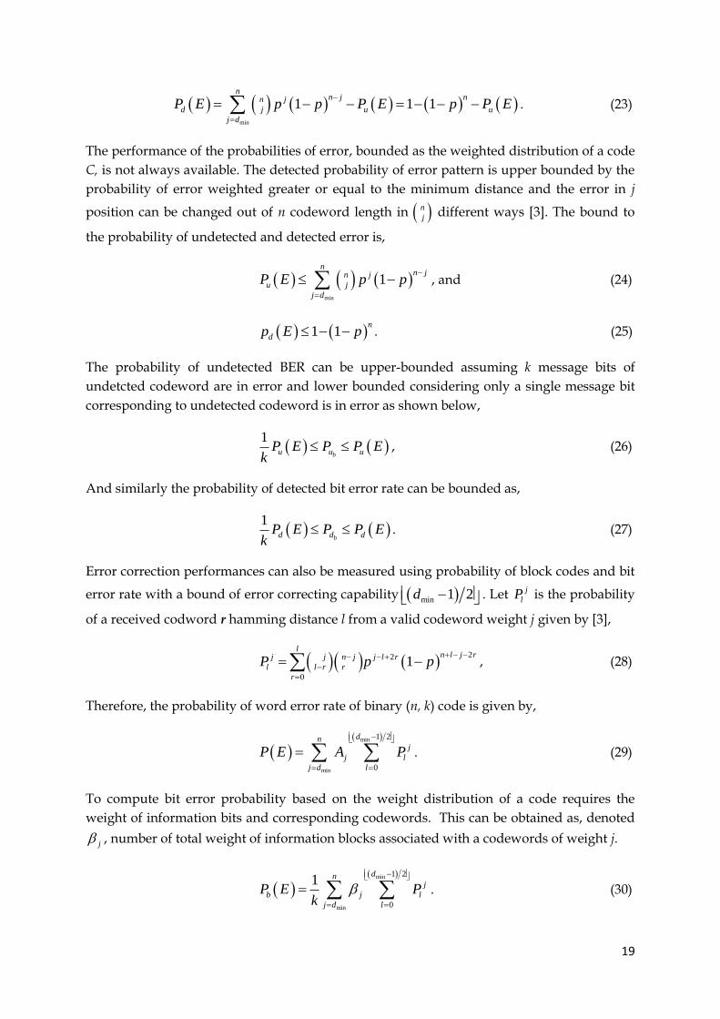
. (23)

The performance of the probabilities of error, bounded as the weighted distribution of a code

C, is not always available. The detected probability of error pattern is upper bounded by the

probability of error weighted greater or equal to the minimum distance and the error in j

position can be changed out of n codeword length in n

j different ways [3]. The bound to

the probability of undetected and detected error is,

min

1n

n jn j

u j

j d

P E p p

, and (24)

1 1n

dp E p . (25)

The probability of undetected BER can be upper-bounded assuming k message bits of

undetcted codeword are in error and lower bounded considering only a single message bit

corresponding to undetected codeword is in error as shown below,

1

bu u uP E P P Ek

, (26)

And similarly the probability of detected bit error rate can be bounded as,

1

bd d dP E P P Ek

. (27)

Error correction performances can also be measured using probability of block codes and bit

error rate with a bound of error correcting capability min 1 2d . Let j

lP is the probability

of a received codword r hamming distance l from a valid codeword weight j given by [3],

22

0

1l

n l j rj j n j j l r

l l r r

r

P p p

, (28)

Therefore, the probability of word error rate of binary (n, k) code is given by,

min

min

1 2

0

dnj

j l

j d l

P E A P

. (29)

To compute bit error probability based on the weight distribution of a code requires the

weight of information bits and corresponding codewords. This can be obtained as, denoted

j , number of total weight of information blocks associated with a codewords of weight j.

min

min

1 2

0

1dn

j

b j l

j d l

P E Pk

. (30)

20

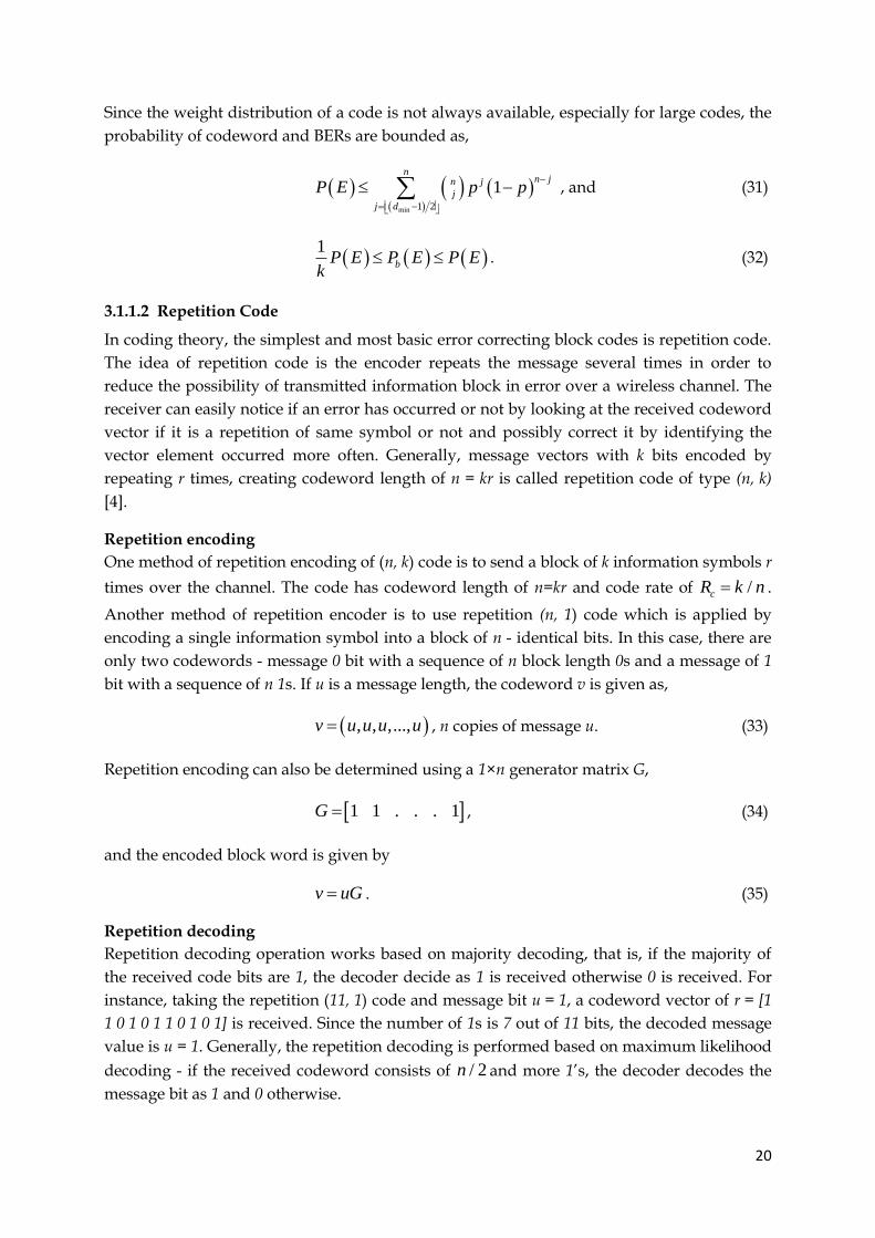
Since the weight distribution of a code is not always available, especially for large codes, the

probability of codeword and BERs are bounded as,

min 1 2

1n

n jn j

j

j d

P E p p

, and (31)

1

bP E P E P Ek

. (32)

3.1.1.2 Repetition Code

In coding theory, the simplest and most basic error correcting block codes is repetition code.

The idea of repetition code is the encoder repeats the message several times in order to

reduce the possibility of transmitted information block in error over a wireless channel. The

receiver can easily notice if an error has occurred or not by looking at the received codeword

vector if it is a repetition of same symbol or not and possibly correct it by identifying the

vector element occurred more often. Generally, message vectors with k bits encoded by

repeating r times, creating codeword length of n = kr is called repetition code of type (n, k)

[4].

Repetition encoding

One method of repetition encoding of (n, k) code is to send a block of k information symbols r

times over the channel. The code has codeword length of n=kr and code rate of /cR k n .

Another method of repetition encoder is to use repetition (n, 1) code which is applied by

encoding a single information symbol into a block of n - identical bits. In this case, there are

only two codewords - message 0 bit with a sequence of n block length 0s and a message of 1

bit with a sequence of n 1s. If u is a message length, the codeword v is given as,

, , ,...,v u u u u , n copies of message u. (33)

Repetition encoding can also be determined using a 1×n generator matrix G,

1 1 . . . 1G , (34)

and the encoded block word is given by

v uG . (35)

Repetition decoding Repetition decoding operation works based on majority decoding, that is, if the majority of

the received code bits are 1, the decoder decide as 1 is received otherwise 0 is received. For

instance, taking the repetition (11, 1) code and message bit u = 1, a codeword vector of r = [1

1 0 1 0 1 1 0 1 0 1] is received. Since the number of 1s is 7 out of 11 bits, the decoded message

value is u = 1. Generally, the repetition decoding is performed based on maximum likelihood

decoding - if the received codeword consists of / 2n and more 1’s, the decoder decodes the

message bit as 1 and 0 otherwise.

21

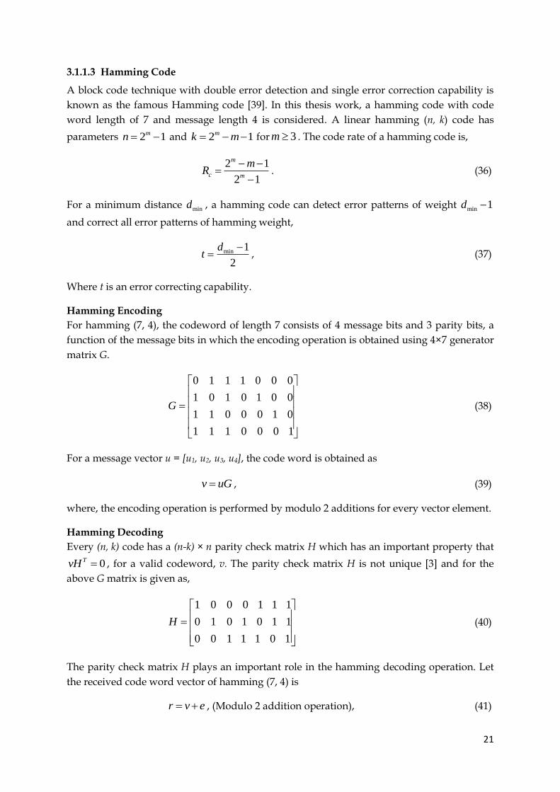
3.1.1.3 Hamming Code

A block code technique with double error detection and single error correction capability is

known as the famous Hamming code [39]. In this thesis work, a hamming code with code

word length of 7 and message length 4 is considered. A linear hamming (n, k) code has

parameters 2 1mn and 2 1mk m for 3m . The code rate of a hamming code is,

2 1

2 1

m

c m

mR

. (36)

For a minimum distance mind , a hamming code can detect error patterns of weight min 1d

and correct all error patterns of hamming weight,

min 1

2

dt

, (37)

Where t is an error correcting capability.

Hamming Encoding

For hamming (7, 4), the codeword of length 7 consists of 4 message bits and 3 parity bits, a

function of the message bits in which the encoding operation is obtained using 4×7 generator

matrix G.

0 1 1 1 0 0 0

1 0 1 0 1 0 0

1 1 0 0 0 1 0

1 1 1 0 0 0 1

G

(38)

For a message vector u = [u1, u2, u3, u4], the code word is obtained as

v uG , (39)

where, the encoding operation is performed by modulo 2 additions for every vector element.

Hamming Decoding

Every (n, k) code has a (n-k) × n parity check matrix H which has an important property that

0TvH , for a valid codeword, v. The parity check matrix H is not unique [3] and for the

above G matrix is given as,

1 0 0 0 1 1 1

0 1 0 1 0 1 1

0 0 1 1 1 0 1

H

(40)

The parity check matrix H plays an important role in the hamming decoding operation. Let

the received code word vector of hamming (7, 4) is

r v e , (Modulo 2 addition operation), (41)

22

where e is the error vector of length 7 and v is the valid codeword. One of the decoding

operations is to compute syndrome in order to detect an error.

T T T T Ts rH v e H vH eH eH . (42)

The syndrome determines if there is an error occurred in the received vector or not. If the

vector s is all zeros, error has not been occurred and the received vector is the valid code

word, otherwise, error occurred and has to be corrected. From the above syndrome Ts eH ,

if a single error has occurred, the error vector will be all zeros except 1 in the position where

the error occurred. Therefore, the syndrome s will be the one of the ith column vector of the

parity check matrix H where the error has occurred. Since all the column vectors of H have

distinct combination of three bits none zero vector, it is easy to identify the error location

based on the syndrome vector and corresponding H matrix column vectors. Generally,

hamming (7, 4) decoding operation has three steps.

Step 1. Compute the syndrome Ts rH from the received vector r and parity check matrix H.

Step 2. Check the value of vector s . If 0s then an error has not occurred and the received

vector is the valid transmitted code word. Else if 0s , error has occurred and need to be

corrected.

Step 3. Check if the value of vector s matches with the column vectors of H matrix and take

the ith column position of the vector which is the position where an error has occurred. The

estimated error pattern, let be n, will be a vector with the value of its ith position is one and

the rest values are zero.

Step 4. The decoded code word is v r n , which is the transmitted code word.

3.1.1.4 Classic Cyclic Code

Cyclic codes are used for error detection and correction code by employing shift registers

and combinational logical elements [4]. Cyclic codes are one subclass of linear block codes

which utilizes an algebraic coding theory for efficient encoding and decoding algorithms and

has less computational complexity. They are suitable for hardware implementation due to

their rich algebraic structure possession [7].

Cyclic Encoding

For cyclic ,n k code C , let u and v are the corresponding message vector and codeword

vector respectively. The codeword vector consists of k information bits and n k parity bits

and v can be expressed as a polynomial form as shown below.

0 1 1,..., nv v v v 1

0 1 1,..., n

nv x v v x v x

. (43)

A linear block code C is cyclic if a cyclic shift of a codeword is also a codeword [1], that is,

0 1 1, ,..., nv v v v C 1

1 0 2, ,...,n nv v v v C . (44)

23

In polynomial form, cyclic shift by one position, which is denoted by 1v x , is performed

by multiplying it by x and modulo 1nx .

v x C 1mod 1nv x xv x x C (45)

An important property of cyclic code is, all the codeword polynomials are multiplies of

unique polynomial called generator polynomial 0 1 ,..., n k

n kg x g g x g x

with a degree

of n k . One method of cyclic encoding is to use a systematic form of encoding and is given

in the following three steps.

Step 1. Multiply the message polynomial u(x) by xn-1.

Step 2. Divide the message polynomial u(x) xn-1 by generator polynomial of g(x) and the

remainder, let b(x), is simply the parity check polynomial.

Step 3. Finally, the code word polynomial is the combination of the parity check polynomial

b(x) and u(x) xn-1, that is, v(x) = u(x) xn-1 + b(x).

The systematic cyclic encoding can also be realized using shift registers and logical elements

called shift register encoder. The encoder circuit is shown in the Figure 7 below.

Figure 7. Shift Register Encoder.

In the beginning, the gate is ON and the k bits of message word are feed to the channel and

then, gate OFF and the register values are shifted in to the channel to form a valid codeword.

In general, the following procedures describe how shift register encoder operates.

Step 1. The message words with a higher order bit enters to the register first and the output

stage simultaneously. The gate is enabled in order to allow feedback for the message bits in

bn-k-1

Gate

v1,v2...vn

u1, u2 ….. uk

b2 b0 + + + +

g0 gn-k-1 g1

Switch

A

B

24

to n-k stage of encoding shift register during the operation and the switch, a gate to the n -

stage output register, is connected to point B first to allow the message bits move to output

register. This process operates until kth shifts.

Step 2. Right after kth shifts, the gate is disabled and the switch is disconnected from point B

and connected to point A. the n-k parity bits in the shift registers are shifted n-k times and

moved to the n – stage output registers.

Step 3. The number of shifts is equal to n and the output shift register contains n-k parity bits

along with k message bits.

Therefore, the above operation requires n-k linear feedback shift registers and n shift

operations to form a systematic codeword, linear combination of the information and parity

check bits.

Figure 8. Meggitt Decoder for cyclic code [2].

Cyclic Decoding

Cyclic decoding requires the same polynomial division using shift registers as cyclic

encoding besides some additional circuitry to perform error correction and detection. The

Syndrome calculation is an important stage in the process of decoding in error control codes

including Meggitt decoder. Let the received codeword polynomial is,

r(x) = r0 + r1x + r2x2 +, . . . , + rn-1xn-1 = v(x) + e(x), (46)

r(x) v(x)

n-k syndrome shift register (SR)

Error pattern detection Gate 2

S(x)

Gate 1 n-stage input buffer

+

+

g1 gn-k-1

rn-1

Syndrome update

25

where

v(x) = v0 + v1x + v2x2 +, . . . , + vn-1xn-1, (47)

and

e(x) = e0 + e1x + e2x2 +, . . . , + en-1xn-1. (48)

v(x) and e(x) are the valid codeword and error polynomials respectively and the syndrome

polynomial is generated by dividing the received polynomial r(x) by g(x) [2]. This is done the

same as the cyclic encoder, n-k shift register are required to perform the division operation of

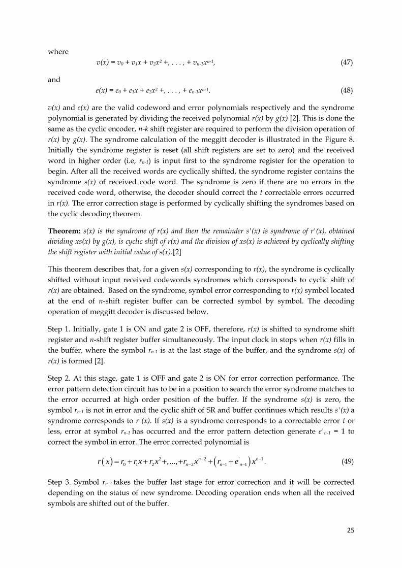
r(x) by g(x). The syndrome calculation of the meggitt decoder is illustrated in the Figure 8.

Initially the syndrome register is reset (all shift registers are set to zero) and the received

word in higher order (i.e, rn-1) is input first to the syndrome register for the operation to

begin. After all the received words are cyclically shifted, the syndrome register contains the

syndrome s(x) of received code word. The syndrome is zero if there are no errors in the

received code word, otherwise, the decoder should correct the t correctable errors occurred

in r(x). The error correction stage is performed by cyclically shifting the syndromes based on

the cyclic decoding theorem.

Theorem: s(x) is the syndrome of r(x) and then the remainder s'(x) is syndrome of r'(x), obtained

dividing xs(x) by g(x), is cyclic shift of r(x) and the division of xs(x) is achieved by cyclically shifting

the shift register with initial value of s(x).[2]

This theorem describes that, for a given s(x) corresponding to r(x), the syndrome is cyclically

shifted without input received codewords syndromes which corresponds to cyclic shift of

r(x) are obtained. Based on the syndrome, symbol error corresponding to r(x) symbol located

at the end of n-shift register buffer can be corrected symbol by symbol. The decoding

operation of meggitt decoder is discussed below.

Step 1. Initially, gate 1 is ON and gate 2 is OFF, therefore, r(x) is shifted to syndrome shift

register and n-shift register buffer simultaneously. The input clock in stops when r(x) fills in

the buffer, where the symbol rn-1 is at the last stage of the buffer, and the syndrome s(x) of

r(x) is formed [2].

Step 2. At this stage, gate 1 is OFF and gate 2 is ON for error correction performance. The

error pattern detection circuit has to be in a position to search the error syndrome matches to

the error occurred at high order position of the buffer. If the syndrome s(x) is zero, the

symbol rn-1 is not in error and the cyclic shift of SR and buffer continues which results s'(x) a

syndrome corresponds to r'(x). If s(x) is a syndrome corresponds to a correctable error t or

less, error at symbol rn-1 has occurred and the error pattern detection generate e'n-1 = 1 to

correct the symbol in error. The error corrected polynomial is

2 2 ' 1

0 1 2 2 1 1,..., n n

n n nr x r r x r x r x r e x

. (49)

Step 3. Symbol rn-2 takes the buffer last stage for error correction and it will be corrected

depending on the status of new syndrome. Decoding operation ends when all the received

symbols are shifted out of the buffer.

26

In practice, the syndrome update in the Figure 8 above is not essential and if it is used the SR

will be zero at the end of the decoding. If it is not considered, the SR will generally be non-

zero after the decoding even though the operation is still correct [2]. One of the advantages of

meggitt decoder is, it computes the syndrome of all correctable error patterns and

corresponding error syndromes, and avoids the required syndrome table. The best way to

elaborate this is using example.

A meggitt decoder of cyclic (15, 7) double error correcting code with a generator polynomial

of g(x) = 1 + x4 + x6 + x7 + x8 can correct up to 15

1 15C single errors and 15

2 105C double

errors. Total of 120 error patterns and their syndromes are required to be stored in case of

syndrome table decoding. The decoder only needs 15 error patterns and corresponding

syndromes as shown in the Table 4 and the rest error patterns and their syndromes can be

determined by cyclic shift of the 15 error patterns. For instance, from the error pattern in the

second row of Table 4 can be obtained using the following error patterns with two successive

errors.

(0000 0000 0000 110)

(0000 0000 0001 100)

(0000 0000 0011 000)

(0110 0000 0000 000)

(1100 0000 0000 000)

(1000 0000 0000 001)

Table 4. Syndrome table of meggitt decoder for cyclic (15, 7) code

No. Error pattern Error syndrome

1 0 0 0 0 0 0 0 0 0 0 0 0 0 0 1 0 0 0 0 0 0 0 1

2 0 0 0 0 0 0 0 0 0 0 0 0 0 1 1 0 0 0 0 0 0 1 1

3 0 0 0 0 0 0 0 0 0 0 0 0 1 0 1 0 0 0 0 0 1 0 1

4 0 0 0 0 0 0 0 0 0 0 0 1 0 0 1 0 0 0 0 1 0 0 1

5 0 0 0 0 0 0 0 0 0 0 1 0 0 0 1 0 0 0 1 0 0 0 1

6 0 0 0 0 0 0 0 0 0 1 0 0 0 0 1 0 0 1 0 0 0 0 1

7 0 0 0 0 0 0 0 0 1 0 0 0 0 0 1 0 1 0 0 0 0 0 1

8 0 0 0 0 0 0 0 1 0 0 0 0 0 0 1 1 0 0 0 0 0 0 1

9 0 0 0 0 0 0 1 0 0 0 0 0 0 0 1 1 1 0 1 0 0 0 0

10 0 0 0 0 0 1 0 0 0 0 0 0 0 0 1 0 1 1 1 0 0 1 0

11 0 0 0 0 1 0 0 0 0 0 0 0 0 0 1 1 1 1 0 0 1 1 1

12 0 0 0 1 0 0 0 0 0 0 0 0 0 0 1 0 0 0 1 1 1 0 0

13 0 0 1 0 0 0 0 0 0 0 0 0 0 0 1 0 0 1 1 1 0 1 1

14 0 1 0 0 0 0 0 0 0 0 0 0 0 0 1 0 1 1 1 0 1 0 1

15 1 0 0 0 0 0 0 0 0 0 0 0 0 0 1 1 1 1 0 1 0 0 1

27

The required error patterns of meggitt decoder cyclic (15, 7) double error correcting code can

be further reduced by cyclic shifting an error pattern in order to obtain other error pattern.

For example, the error pattern in the second row entry is cyclically shifted to the right to get

error pattern in the last entry of the table. Applying in the same way, the 14 double error

patterns can be simplified to 7 error patterns and corresponding error syndromes. Each and

every error pattern requires its own syndrome detection circuit and one of the drawbacks of

meggitt decoder is its complexity and cost as the error correcting capability t increases.

3.1.1.5 BCH Codes BCH codes are subclass of cyclic codes that possess a rich algebraic structure for efficient

algebraic decoding algorithms [6]. In this section, a binary BCH code with a block length of

2 1mn for integer 3m is presented. A binary BCH code with error correcting capability 12mt and positive integer 3m can be designed using the following relations [6],

min

2 1

2 1

mn

n k mt

d t

(50)

BCH (n, k, mind ) code with the above requirements which determines the block length n,

bound on n-k parity check bits and the minimum error correcting capability t is called a t –

error correcting BCH code.

A BCH code fulfill the above specified relations is a cyclic code whose generator polynomial

g(x) has 2t roots 2 3 4 2, , , ,..., t . Therefore, a BCH (n, k, mind ) code has a generator

polynomial of degree at most mt and divisible by minimum polynomial i x for1 2i t

given by [6],

,1 2ig x LCM x i t . (51)

LCM represents the least common multiple of the minimum polynomials i x .

Figure 9. BCH decoder with 2mGF arithmetic operations [5].

r(x)

v(x)

Syndrome

computation

Compute

error location

polynomial

Find error

positions

Delay RAM (processing element) +

Error

estimation

28

BCH encoding

As BCH (n, k) code is a large class of cyclic codes, its encoding procedures are quite similar to

the cyclic encoding discussed above. For a given generator polynomial g(x), the information

polynomial u(x) is multiplied by n kx , that is, n kx u x . It is then divided by the generator

polynomial where its reminder will be the parity check polynomial b(x). Finally the check

polynomial b(x) is added to n kx u x in order to obtain the codeword polynomial v(x).

BCH decoding

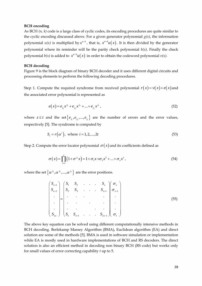
Figure 9 is the block diagram of binary BCH decoder and it uses different digital circuits and

processing elements to perform the following decoding procedures.

Step 1. Compute the required syndrome from received polynomial r x v x e x and

the associated error polynomial is represented as

1 2

1 2... z

z

j j j

j j je x e x e x e x , (52)

where z t and the set 1 2, ,...,

zj j je e e are the number of errors and the error values,

respectively [5]. The syndrome is computed by

i

iS r , where 1,2,...,2i t (53)

Step 2. Compute the error locator polynomial x and its coefficients defined as

2

1 2

1

1 1 ...l

zj z

z

l

x x x x x

, (54)

where the set 1 2, ,..., zj j j are the error positions.

1 1 2

2 2 3 1 1

2 1 2 1 1

. . .

. . .

. . . . . .

. . . . . .

. . . . . .

. . .

z z z

z z z

z z z z

S S S S

S S S S

S S S S

(55)

The above key equation can be solved using different computationally intensive methods in

BCH decoding. Berlekamp Massey Algorithm (BMA), Euclidean algorithm (EA) and direct

solution are some of the methods [5]. BMA is used in software simulation or implementation

while EA is mostly used in hardware implementations of BCH and RS decoders. The direct

solution is also an efficient method in decoding non binary BCH (RS code) but works only

for small values of error correcting capability t up to 5.

29

The BMA algorithm uses iterative procedure approach to build the Linear Feedback Shift

Register (LFSR) structure with tabs 1 2, ,..., t and output syndrome sequences S1, S2, . . . ,

S2t as shown in Figure 10 [5].

Figure 10. Linear Feedback Shift Register (LFSR)

The main target of BMA is to find a polynomial 1i x of minimal degree that satisfies (56)

[5].

1

1

0

0il

i

k j j

j

S

, 1il k i . (56)

(56) is equivalent to 1

1

1 1 1

11 ... i

i

li i i

lx x x

be the LFSR connection polynomial that

gives partial sequence of syndromes [5].

The discrepancy at iteration i is given by,

1 1 1...i i

i i

i i i i l ld S S S . (57)

This discrepancy value contains a correction term to compute and modify 1i in the next

iteration. It is also used to measure how good the LFSR structure outputs the syndrome

sequences. The algorithm works base on the following two conditions:

If di = 0 then

1i tx x , 1i il l . (58)

If 0id , the solution for iteration = b is let b x such that 1 , 0bb i d , and bb l is

maximal. And then

1 1i i i b b

i bx x d d x x ,

j = z+1, z+2, . . . , 2z

+ + +

30

and 1 max ,i i bl l l i b . (59)

To begin the iteration procedure i = 0, the initial conditions of BMA algorithm are given by

[5]

11x

, 1 0l ,

1 1d ,

and 01x , 0 0l , 0 1d S . (60)

The computation of error location polynomial 1i x continues such that the conditions

1 1ii l t or 2 1i t , or both conditions are fulfilled [5].

Step 3. Calculate the inverses of the roots of x , which is the errors location using chien

search algorithm. So far, the syndrome is used to determine the error location polynomial

x and now it is time to determine the roots of x based on trial and error procedures.

All non-zero elements of 2mGF that is, the sequences 2 11, , ,..., n are generated to

evaluate the condition 1 0 [5]. The multiplicative inverse of the roots are used to

identify the location of the errors, 1 2, ,..., zj j j , therefore, once the exact error positions

1 2, ,..., vj j j are determined, the corresponding received bits in the buffer or delay RAM is

complemented to correct the errors.

3.1.1.6 Reed-Solomon code

RS codes are interpreted as non-binary BCH codes in which the code coefficient values are

obtained from 2mGF . The generator polynomial g(x) of RS code with t error correcting

capability is given by the product of minimal polynomials of the elements i where i = 1, 2,

… , 2t, 2mGF . The elements 2 2, ,..., t are the roots of generator polynomial g(x)

and computed as,

2 2... tg x x x x (61)

Reed-Solomon encoding

RS encoding follows the same procedure as BCH encoder does and is given as follows.

Step 1. Multiply the information polynomials by 2tx and yields 2tx u x

Step 2. Divide it by generator polynomial g(x)

Step 3. Obtain the reminder of 2tx u x / g(x) which is the parity check polynomial and

combine the product and check polynomial to get RS code word symbols.

Reed-Solomon decoding

The RS decoding procedure is similar to binary BCH decoding algorithms only the error

values has to be computed in the case of RS code. The general decoding procedure of RS

code is given in Figure 11.

31

Figure 11. RS decoder with 2mGF arithmetic operations [5].

Step 1. Compute the syndrome sequences using (equation form BCH).

Step 2. Find the error location polynomial and its coefficient values applying the above

computationally efficient methods, such as BMA, EA and Direct solution.

Step 3. Use chien search procedure to find the error locators, that is, the roots of error

location polynomials.

Step 4. Compute the error values,lj

e , 1 l z , for z t . The error values can be evaluated

below.

2

'

l l

l l

j j

j je

, (62)

Where ˡ(x) is the derivation of error location polynomial x with respect to x and the

expression x is called error evaluator polynomial given as,

2 1mod tx x S x x (63)

Step5. Correct the errors by adding the computed error values to the received symbols over

2mGF .

3.1.2 LDPC and Turbo Codes

LDPC and Turbo codes are a high performance FEC codes which are applied to approach

capacity channel, that is, by increasing the code rate, reliable communication is achievable in

a given noise level. Nowadays, LDPC and Turbo codes are competing to each other due to

their similar performance.

3.1.2.1 LDPC Code

LDPC is a forward error control code with a parity check matrix contains very small number

of non-zero entries [59]. The sparseness property of H-matrix of LDPC code guarantees the

complexity of the decoder and minimum distance which both increase linearly with the

r(x)

e(x)

v(x)

Syndrome

computation

Compute

error location

polynomial

Find error

positions

Delay RAM (processing element) +

Find the error

values

32

length of codeword. The biggest difference of LDPC code from block codes is in its iterative

decoding operation that uses graphical representation of H-matrix [59].

LDPC Encoding

For encoding technique, the generator matrix G can be found by first obtaining H matrix in

the form of

, n kH A I , (64)

where A is a binary matrix of n k k dimension and n kI is n k identity matrix.

Therefore, the generator matrix G is,

, T

kG I A (65)

The G matrix is not as sparse as the H matrix and it is very large in size. The encoder

operation is performed simply by multiplying the information vector u with G matrix [59],

c uG (66)

LDPC Decoding

There are two types of iterative decoding in LDPC code called hard and soft decision

decoding. There are common LDPC decoding algorithms such as bit–flipping, sum-product

and min-sum algorithm to mention a few. The bit-flipping algorithm is one of the LDPC

decoding techniques, which is a hard decision message-passing algorithm [59]. This

algorithm is the LDPC decoding technique that we focus on in our thesis. It is shown that

parity check H matrix can be represented using a Tanner graph which has two classes of

nodes. The first class, is called code nodes corresponds to bit nodes to columns of H. for

instance, for (n – k) × n parity matrix H, we have n code nodes. The second class is called

check nodes correspond to parity check equations to the rows of H matrix and we have n – k

check nodes for (n – k) × n parity matrix H.

The bit-flipping algorithm is given as follows,

Step 1: messages of the check nodes are calculated based on the received codeword and

information available in the check matrix.

Step 2: the check node sends messages to the connected code nodes.

Step 3: the bit node checks the messages from the check node and if the majority of message

bits in the first bit node are different from the received bit, the bit node flips its value. And

this procedure continues for all values of bit nodes.

Step 4: the parity check equations are calculated, that is, all the check nodes are determined

using modulo-2 sum and check if all satisfy the sum of the bit values is zero. If it is satisfied

the algorithm halts, otherwise, the procedure is repeated till all the parity check equations of

the check nodes are fulfilled or till the maximum iteration has reached.

3.1.2.2 Turbo Code

In this sub-section, we will concentrate on a Maximum A Posteriori (MAP) based turbo code.

A turbo code with a rate of 1/3 is considered as shown in Figure 12. From Figure 12, the

33

upper case variables denote the binary numbers while the lower case variables denote the

symbol values. In the transmitter part, a pair of convolutional encoders generates pair of

parity bits for the corresponding message bits and mapped to symbols for transmission over

Additive White Gaussian Noise (AWGN) channel.

kX = message bits 2 = noise variance

1kP = encoder 1 parity bit '

kx = received message symbol

2kP = encoder 2 parity bit '

1kp = received encoder 1 parity symbol

kx = message symbols '

2kp = received encoder 2 parity symbol

1kp = encoder 1 parity symbol kL x = decoder soft decision

2kp = encoder 2 parity symbol ^

kX = decoder hard decision

Figure 12. Turbo code system [60]

Turbo Encoding

Two identical convolutional encoders are applied for the structure of turbo encoder with a

rate of 1/3 as shown in Figure 13. The information bits are fed directly to the first

convolutional encoder and it also go through a pseudo random permutation P before it is fed

to the second convolutional encoder. The permutation block is used based on the state

sequence of a maximal length shift register (PN sequence) and its benefit is to make the two

constituent encoders be uncorrelated at the receiver side [60].

Figure 13. Turbo Encoder

encoder Map bits to

symbols decoder slice

kX

1 2, ,k k kX P P 1 2, ,k k kx p p

' ' '

1 2, ,k k kx p p kL x ^

kX

20,N

Convolutional encoder 1

Convolutional encoder 2

P

1kP

kX

kx

2kP

34

Each convolutional encoder in Figure 13 is based on recursive systematic convolutional

encoder and it is shown in Figure 14 with two memory registers and four states.

Figure 14. Recursive systematic convolutional code

Turbo Decoding

The turbo decoder consists of a pair of decoders as shown in figure 15. The two decoders

work cooperatively to enhance and improve the estimation of the original information bits.

The decoders operate based on maximum aposteriori probability (MAP) algorithm which

minimizes the probability of bit error by using the entire received sequence to identify the

most probable bit at each stage of the trellis. In this case, the soft decision information

learned from the noisy received parity bits.

Initially, the first encoder begins without initialization information (apriori estimates are set

to zero). In next iterations of the decoding process, the soft decision information of one MAP

decoder is used as the apriori information to initialize the other MAP decoder. The decoder

information is cycled around the loop until the soft decisions converge to a steady state

solution (stable set of values). The latter soft decisions are then sliced to recover the original

binary sequence.

Figure 15. Turbo decoder [60]

0u 1u

nX

1 0state u u

nP

nX

MAP

decoder 1

MAP

decoder 2

P

P

P-1

'

1kp

'

kx

1

e kL x

2

e kL x

'

kx

'

2kp

35

3.2 Introduction to ARM Platform

ARM (Advanced RISC Machine) is world’s leading supplier of embedded microprocessors

technology. It is a 32-bit architecture which offers a wide range of microprocessor cores to

address high performance, low cost, low computing power consumption and small

implementation size. The ARM processor architecture is the basis for every ARM processors

and is evolved over time to include additional features in order to encounter the growing

demand of new functionality, high performance and the need of new and emerging market.

The ARM architecture incorporates the following similar features of Reduced Instruction Set

Computer (RISC) architecture:

A large register file

A uniform register file load/store architecture, where the data processing operation is

performed only on register contents, not directly on the memory contents

Uniform and fixed length instruction fields, a 16 × 32- bit register files

Simple addressing mode, all load/store addresses obtained from instruction fields

and register contents only

ARM enhances the basic features of RISC by enabling the processors to achieve the key

attributes of ARM architecture [8]:

Good balance of high performance

Small code size

Low power consumption

Small silicon area

ARM also provides a series of ARM core technologies, architecture extensions and system-

on-chip schemes. ARM CPU core includes a series of processor family, such as Cortex-A,

Cortex-R, Cortex-M, ARM7, ARM9, ARM11 and SecurCore. The ARM Cortex-M is a group

of 32-bit RISC processor cores upward compatible range of energy efficient, easy to use

processors designed to achieve the demands of future embedded applications such as

increase connectivity, better code reuse, lower cost and enhanced energy efficiency [8]. This

family is optimized for cost and power sensitive embedded microcontrollers (MCU), and

mixed signal devices applications, automotive and control systems, medical instrumentation

and smart metering are few to mention.

Cortex-M3 processor is a member of Cortex-M family; it is the industry leading 32-bit

processor delivers high computational performance, energy efficiency, rich connectivity and

execution of instruction set for optimal performance and code size. It is developed to

increase the demand of developing high performance low cost platform for devices

including wireless sensor networks, microcontrollers, industrial control and automotive

systems. The processor clock speed is configurable to 12MHz or 24MHz when using the

crystal oscillator and 6MHz or 12MHz when the integrated high frequency RC oscillator is

used.

36

In this thesis project, the STM32W108cb, IEEE 802.15.4 standard radio, development board

from IAR system is used for our evaluation platform and is shown in Figure 16.

STM32W108cb is a complete System-on-Chip from STMicroelectronics that integrates

2.4GHz IEEE 802.15.4-compliant transceiver, 32-bit ARM Cortex-M3 microprocessor,

128Kbytes embededd flash memory 8Kbytes RAM memory for data and program storage,

and peripherial of use to designers of 802.15.4 based systems [8].

The STM32W108cb tranceiver architecture is chosen for robust co-existance with other

devices in 2.4GHz ISM band channel, namely IEEE 802.11 (WiFi) and Bluetooth, by adopting

channel hopping strategy and minimize power consumption. The timing requirement

imposed by ZigBee and IEEE 802.15.4 standards is maintained by the STM32W108108cb

MAC function which interfaces the on-chip RAM to the receiver and transmitter baseband

modules. The MAC hardware controls automatic ACK transmission and reception, back off

delay, clear channel assessment for transmission, automatic packet level filtering [8].

The STM32W108cb provides advanced power management features to maintain long battery

life time. A high frequency 24MHz external crystal oscillator, 12MHz internal RC oscillator,

32.768KHz external crystal oscillator and 10KHz internal RC oscillator are available. In order

to support user-defined applications a general purpose timers, SPI (master or slave), I 2 C

(master only), UART operations, general purpose ADC and 24 highly configurable GPIOs

are included on chip peripherals. Deep sleep modes to reduce power consumption,

intergrated voltage regulators, 32-bit sleep are also available [9].

The STM32W108cb implements ARM serial wire and JTAG debug interfaces which both

provide real time and debugging capabilities. It also support the standard ARM system

debug capabilities such as Patch and Breakpoint, Data Watchpoint and Trace, and

instrumentation Trace Macrocell application [9].

Due to the above important features, the STM32W108cb is suitable for a wide range of

applications such as,

Smart energy.

Home automation and control.

Building automation and control.

Security and monitoring.

6LoWPAN and custom protocols.

RF4CE products and remote controls.

ZigBee pro wireless sensor networking.

37

Figure 16. STM32W108 application board (MB954)

38

Chapter 4

Implementation and Performance Evaluation

In this section, the FEC codes in IWSNs, the strict requirements that we need to follow,

complexity algorithms of FEC codes, the measurement setup and evaluation results followed

by analysis and discussions will be presented.

4.1 Applying FEC codes in IWSNs

As it is described in the previous chapter, FEC code is an error detection and correction

mechanism used to recover the corrupted data by adding redundancy bits. The redundant

bits are added to original data to form a codeword and correct the erroneous bits caused by

harsh environment. The code rate of FEC code is used to evaluate its transmission efficiency.

FEC code is implemented in IWSN by applying it on top of IEEE 802.15.4 MAC layer. FEC

can be applied on top of PHY layer but we need to have direct interaction to the

manufacturers. Therefore, our task is to concentrate on applying FEC code on top of MAC

layer in an efficient way.

In our project, the feasibility of applying FEC code in IWSNs depends on three important

issues that we need to focus on, namely, the way to properly apply FEC code to a MAC

frame, the encoding and decoding time of FEC codes required to meet the acknowledgement

timing requirement of IEEE 802.15.4 standard and the memory usage of the algorithms in a

resource limited embedded device.

4.1.1 FEC in MAC Layer

In this sub-section, the IEEE 802.15.4 data frame at MAC layer is used as shown in figure 17.

It consists of three main parts: MAC header (MHR), MAC payload and Frame check

sequence (FCS) [10].

Octets 2 1 4 to 20 n 2

Frame

control

Sequence

number

Address field Data payload FCS

Figure 17: IEEE 802.15.4 Data Frame Structure [10]

We propose to encode the frame with FEC code excluding FCS field to encode. The FCS field

contains the cyclic redundancy check (CRC) in order to detect bit errors but not correct them.

The reason not to apply FEC code in FCS field is, firstly, due to the compatibility issue of the

IEEE 802.15.4 as the introduction of redundancy change the packet structure. If the FCS field

is encoded, the calculated FCS value over the whole packet in the standard will not be the

right checksum value, since the packet will be changed after it is encoded. Therefore, nodes

with no FEC code implemented will calculate and obtain different FCS value which will

MAC Payload MFR MHR

MAC

Sublaye

r

39

assume that the packet is corrupted even if it is not. Secondly, it is very convenient when the

receiver decodes the packet if only FCS check is failed in order to avoid unnecessary

computation. If FCS is not encoded, it can be used first to check if the packet is corrupted or

not since its computation is faster than the FEC decoding operation. Moreover, if FCS check

confirms that error is not occurred, the packet decoding is avoided and the receiver fitches

the necessary packet efficiently depending on the encoded packet structure.

For FEC code algorithms, systematic code is the proposed approach. In this case, the code

word consists of original data and additional redundancy which are stored separately in the

payload field without changing the original packet. Furthermore, it is important to add a flag

in the frame control field in the MAC header to indicate that if a packet is encoded or not. In

the systematic approach, if error does not occur, the nodes can easily parse the packet

without applying FEC code. Nodes without FEC scheme implemented can also understand

the content of the encoded packet.

4.1.2 Timing Requirement

The combination of FEC code and ARQ approach is called Hybrid ARQ and used to

guarantee communication reliability and real time performance. If this mechanism is applied

in IWSNs, the timing requirement of the IEEE 802.15.4 standard should be fulfilled. That is,

the macAckWaitDuration is the timing limitation of acknowledgement defined in the

standard. According to the standard, the macAckWaitDuration is 0.864ms and the decoding

time duration of FEC code should reside within this time interval, otherwise, it is not

compatible with the standard. Even in a complicated scenario where the acknowledgement

packet is encoded, the sum of encoding and decoding time should be less than 0.864ms.

Therefore, the encoding and decoding times of FEC algorithms are very essential to meet the

acknowledgement timing requirement of IEEE 802.15.4 standard. This timing requirement is

the key point for the proposed FEC algorithms to be applied in IWSNs and is the metric to be

strictly followed in order to evaluate and compare the algorithms based on the performance.

4.1.3 Memory Resource

The embedded devices in IWSNs are memory resource limited. The microcontroller device

used is integrated with 128Kbyte embedded flash memory and 8Kbyte RAM memory for

data and program storage. Therefore, the FEC algorithms that are going to be implemented

in IWSNs should be feasible in terms of memory resource consumption.

4.2 Complexity Algorithms

The complexity Algorithm is used to determine the amount of resources (time and memory)

consumed to execute certain algorithms that are designed to operate for a given input length.

It is a cost measured in run time (time complexity) or memory (space complexity) required

by an algorithm to solve one of computational problems. In general, the complexity analysis

allows us to measure speed of a program and memory allocation when it performs

computation. In this thesis work, we will only focus on time complexity to analysis the

performance of different FEC schemes.

40

4.2.1 Time Complexity

Time complexity is the measure of running time of a given algorithm as a function of size of

the input. The time complexity of an algorithm is determined using big O notation which

finds a certain bound that the algorithm cannot exceed by excluding factors such as

coefficients and lower order terms. The big O notation is an asymptotic notation used to

express algorithm’s performance as the size of the input tends to infinity. For instance, for

inputs of size n, if the required running time of an algorithm is 43 2 3n n , the asymptotic

time complexity of the algorithm is O 4n .

4.3 Measurement Setup

For our evaluation purpose, the implementation tools and settings used, the software

implementation sources and the methods applied to measure processing time and memory

footprint of each FEC coding algorithms will be introduced.

4.3.1 Implementation Tools and Settings

The IAR embedded Workbench IDE 6.4 is used as our evaluation tool. The IAR Embedded

Workbench provides powerful integrated development environment that allows developing

application projects for embedded systems.

The IAR embedded Workbench IDE is a frame work where all the tools required to build the

application such as, the highly optimizing IAR C/C++ Compiler, assembler, linker, library

tools, editor, project manager and the IAR C-SPY Debugger are integrated.

Except the optimization settings in the C/C++ compiler, the most common default settings

of IAR Embedded Workbench are used. The ARM IAR C/C++ compiler provides you with

an option to optimize the generated code in size, speed or balance in order to reduce code

size (memory) and improve the execution speed performance. This can be fulfilled according

to settings specified in the selectable optimization levels. There are several optimization

levels such as none, low, medium and high (maximum optimization). At each optimization

level, there are different transformations, such as common sub-expression elimination, loop

unrolling, function inlining, code motion, type-based alias analysis, static clustering,

instruction scheduling. In our evaluation, all the transformations are enabled for high level

optimization.

The STM32W108cb supports maximum 24MHz clock frequency and is set to be used for the

evaluation. In the hardware environment set up, the board is connected with a PC using USB

cable through USB connector J2 to give power source to the board and communicate with

hypertherminal use as an output tool. The hypertherminal is configured: word length of 8

bits, one stop bit, no parity, baud rate of 115200 bits per second and disable flow control.

4.3.2 Implementation Sources

A pure C programming software implementation is applied for our evaluation. Neither

assembly nor hardware implementation is performed and an existing demo implementation

project is adapted from ST microcontroller. This demo is an RF application that demonstrates

point-to-point 802.15.4 wireless communication runs on STM32W108cb microcontroller.

41

4.3.3 Methods for Measurement

In our evaluation, memory consumptions and processing time (execution time) performance

are the two main features used to be determined for each error control coding algorithms

and evaluate their performances. The methods used to measure these two features are

discussed as follows.

4.3.3.1 Memory

In embedded systems, memory (flash and RAM memories) is very precious resource.

Understanding and evaluating how our program allocates variables in memory is an

important task to use memory wisely in the area of embedded systems. Memory in a C

program includes code, typically read only and executable instruction, and data which is

non-executable and can be read-only or read-write. The code and read-only data are stored

in flash memory whereas; the read-write data is stored in RAM.

There are two methods used to measure the memory footprint of each error control coding

algorithms. The first method: the IAR Embedded Workbench IDE is set to generate an output

of list file for each C program file whenever the project is compiled. The memory usage of

each algorithm is stated at the end of each list file in three memory types namely, code

memory, const code memory and data memory. The code memory represents the footprint

of executive program in the flash memory and const code memory represents the size of the

initialized constant values of variables in our C program file. The data memory denotes the

size of RAM consumed by our C program file. The second method is the IAR Embedded

Workbench IDE is set in order to generate one of the output files called map file when the

project is compiled. The map file differs from the list file in terms of the memory footprint

and the name of the memory types it represents. It shows the total footprint of the whole

project with different names of memory types from the names in the list file. The memory

types obtained in the map files are; read-only code memory, read-only data memory and

read-write data memory which correspond to memory type in the list file code memory,

const code memory and data memory respectively.

In the first method, each footprint of a particular algorithm can be obtained by reading out

directly from the list files. When the second method is used we have to read the memories in

the map file first before the algorithm of interest is added into the project and read the file

once again after the algorithm is included into the project. Subtracting the memory obtained

after our algorithm is added by the value of corresponding memory before it is added, we

obtain the memory size of our algorithm. The first method seems more convenient and easy

to read the values than the second one. However, the second method is more accurate than

the first one. It is because of not all codes of the algorithm are included in one C file and even

the algorithm includes several C files the size of the algorithm is not obtained by adding up

all the memories obtained from the list files involved. Applying the second method yields

more accurate result as it can obviously be seen when one or more algorithms are added to

the project how much memory it consumes. Therefore, the memory consumption of each

error control coding algorithm is measured using the second method.

42

4.3.3.2 Processing Time

In our evaluation, a system timer (systick) is used to measure the processing time of each

algorithm. System timer is a 24-bit count down timer made available in ARM Cortex-M3

MCU that the processor uses it as a real time operating system tick timer or as a simple

counter. Systick is suitable and very simple to generate ticks for operating system or delay

measurement. When MCU runs a program, an instruction is executed at a given speed by the

system clock. Some execution of instruction may take one clock cycle and others may take

more to complete the execution. Systick can be used to determine the elapsed time by setting

the timer to start down counting. The measured units in systick method are number of ticks

not CPU cycles.

Therefore, the performances of our algorithms are measured using systick timer by first

initializing and starting the systick timer. The systick timer source clock in STM32W108cb is

specified to two clock frequencies, 12MHz and 24MHz. The 24MHz frequency is used as a

clock source and some extra line of codes for measurement applying systick timer. The

systick values are read out before and after the test point of our interest and take their

difference to get the tick values. The time consumption is calculated by dividing the tick

values with the clock speed frequency.

In order to guarantee the systick timer measurement is accurate, an oscilloscope is used to

verify which shows the method is correct. For instance, the delay of one second between two

blinking LEDs is measured using systick timer with the above procedures. And an

oscilloscope is used to check the one second delay to blink the two LEDs in the board, and

their voltage and time is shown in the Figure 18.

Figure 18. Voltage of LEDs

43

4.4 Performance Evaluation

In this subsection, the results of our evaluation are presented. The purpose of our evaluation

is to measure the processing time of FEC codes and identify an appropriate algorithm for

IWSNs. The evaluation of footprint of the algorithms is also crucial factor to be considered as

the IWSN nodes are memory resource limited embedded devices. Therefore, processing time

and memory consumptions are two important factors to be measured in our evaluation

using the two techniques introduced previously in order to identify the feasible FEC

algorithms applicable in IWSNs. Some block codes are proposed for our evaluation purpose

as they are suitable for data link layer compared to convolutional codes due to their

memoryless property. Turbo and LDPC codes are also considered to show their performance

in IWSNs and compare with block codes.

In our evaluation, we use a development kit from STMicroelectronics with high performance

32-bit ARM Cortex-M3 microprocessor operating at 24MHz frequency. The IAR Embedded

Workbench 6.4 compiler that supports four optimization levels uses high level of

optimization in order to achieve better performance interms of processing time and memory

consumptions. A pure C language software is applied for our implementation and is not

optimal. One can further optimize to improve the perfromance interms of execution time and

memory footprint. In IWSNs the maximum payload of IEEE 802.15.4 standard is 128 bytes

and, therefore, the maximum data length is considered in order to assess at the worst case

senario: maximum latency and memory consumption. the encoded data length using FEC

algorithms must be less than 128 bytes and the orginal message length should even be

shorter. The maximum packet size of the original message depends on the code rate of FEC

code which is caluculated as, max 128L R .

The memory usages of each FEC algorithms are presented and classified into three memory

regions, that is, Read-Only (RO) code memory, RO data memory and Read-Write (RW) data

memory. As we discussed in the previous subsection, RO code memory represents the size of

executable program, RO data memory represents the size of initialized constant values and

RW data memory represents the size of RAM the algorithm uses. The memory footprint of

our algorithms is measured using different compiler optimization options such as high

speed, high size, high balance and none optimizations.

The processing time of our evaluation is also presented in three different sections: encoding

time, decoding time without error and decoding time with maximum correctable error. The

maximum correctable error means that a packet encounters the maximum number of errors

that the corresponding FEC algorithm can correct them. Hence, the execution time of FEC

decoding without error and with maximum errors are not the same and should be presented

separately. Each sections are also measured by applying different optimization levels such as

high speed, high size, high balance and none optimzation options.

The evaluation results are categorized into two parts, namely, evaluation results of block

codes and evaluation results of LDPC, turbo and block codes each followed by analysis and

discussions of the results.

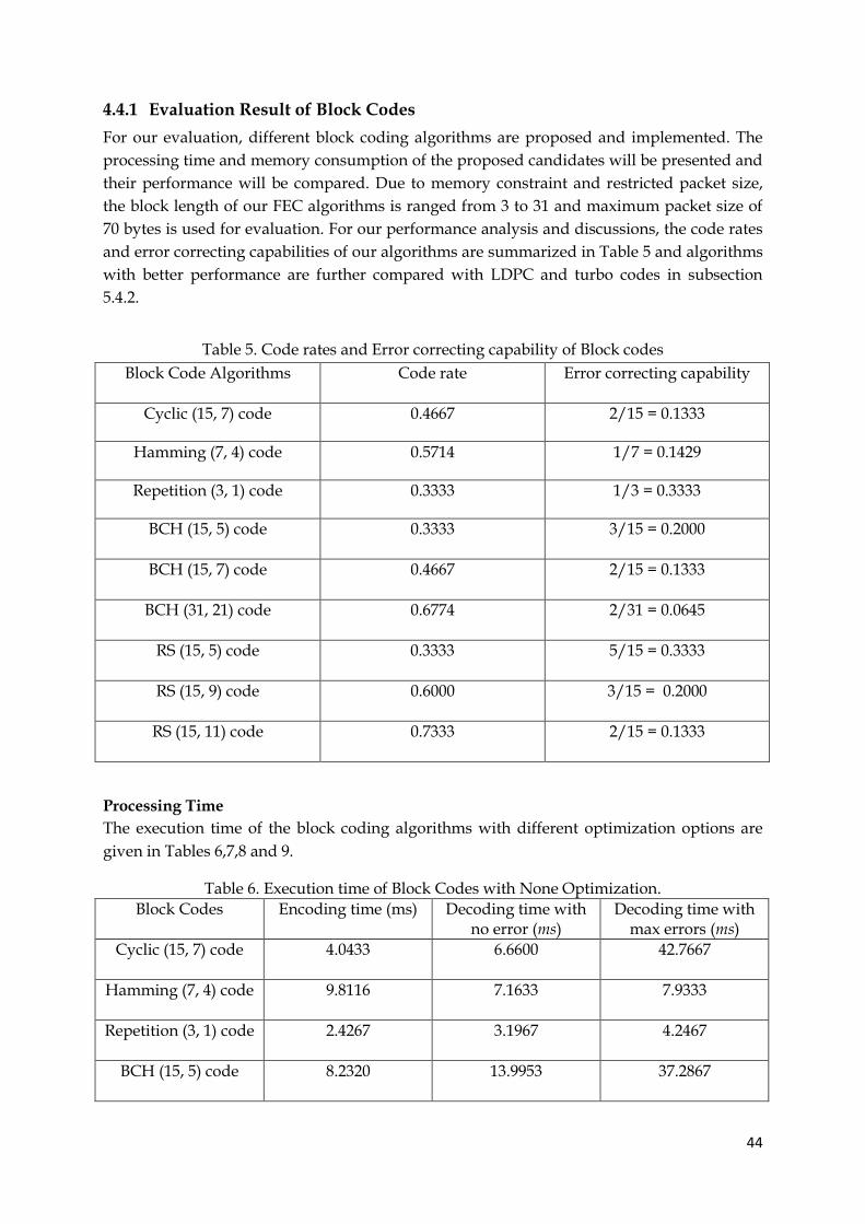
44

4.4.1 Evaluation Result of Block Codes

For our evaluation, different block coding algorithms are proposed and implemented. The

processing time and memory consumption of the proposed candidates will be presented and

their performance will be compared. Due to memory constraint and restricted packet size,

the block length of our FEC algorithms is ranged from 3 to 31 and maximum packet size of

70 bytes is used for evaluation. For our performance analysis and discussions, the code rates

and error correcting capabilities of our algorithms are summarized in Table 5 and algorithms

with better performance are further compared with LDPC and turbo codes in subsection

5.4.2.

Table 5. Code rates and Error correcting capability of Block codes

Block Code Algorithms

Code rate Error correcting capability

Cyclic (15, 7) code 0.4667 2/15 = 0.1333

Hamming (7, 4) code 0.5714 1/7 = 0.1429

Repetition (3, 1) code 0.3333 1/3 = 0.3333

BCH (15, 5) code

0.3333 3/15 = 0.2000

BCH (15, 7) code

0.4667 2/15 = 0.1333

BCH (31, 21) code

0.6774 2/31 = 0.0645

RS (15, 5) code

0.3333 5/15 = 0.3333

RS (15, 9) code

0.6000 3/15 = 0.2000

RS (15, 11) code

0.7333 2/15 = 0.1333

Processing Time

The execution time of the block coding algorithms with different optimization options are

given in Tables 6,7,8 and 9.

Table 6. Execution time of Block Codes with None Optimization.

Block Codes

Encoding time (ms) Decoding time with no error (ms)

Decoding time with max errors (ms)

Cyclic (15, 7) code

4.0433 6.6600 42.7667

Hamming (7, 4) code

9.8116 7.1633 7.9333

Repetition (3, 1) code

2.4267 3.1967 4.2467

BCH (15, 5) code

8.2320 13.9953 37.2867

45

BCH (15, 7) code

7.0967 5.3700 16.2233

BCH (31, 21) code

8.9741 3.3356 9.4185

RS (15, 5) code

4.2280 10.8395 30.7020

RS (15, 9) code

2.1613 3.8107 9.3040

RS (15, 11) code

1.6813 2.4245 4.9362

Table 7. Execution time of Block Codes with High Speed Optimization

Block Code Algorithms

Encoding time (ms) Decoding time with no error (ms)

Decoding time with max errors (ms)

Cyclic (15, 7) code

1.6333 3.0067 35.6833

Hamming (7, 4) code

2.4500 2.4908 3.1383

Repetition (3, 1) code

0.5133 1.5167 2.8000

BCH (15, 5) code

2.0020 5.9033 16.9027

BCH (15, 7) code

1.4633 2.8333 8.1267

BCH (31, 21) code

2.4424 1.7044 4.4854

RS (15, 5) code

1.4268 4.6025 13.9965

RS (15, 9) code

0.6333 1.6220 4.3787

RS (15, 11) code

0.5953 0.9582 2.3454

Table 8. Execution time of Block Codes with High Size Optimization

Block Code Algorithms

Encoding time (ms) Decoding time with no error (ms)

Decoding time with max errors (ms)

Cyclic (15, 7) code

2.3600 7.4967 33.7533

Hamming (7, 4) code

6.4867 5.6642 6.1192

Repetition (3, 1) code

1.7733 2.3100 3.2667

BCH (15, 5) code

3.7287 11.3260 21.0047

BCH (15, 7) code

3.1833 3.8033 9.1500

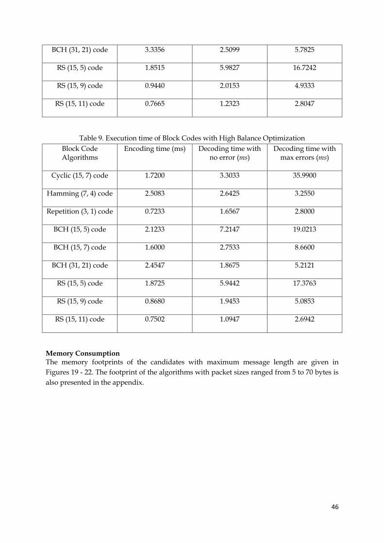
46

BCH (31, 21) code

3.3356 2.5099 5.7825

RS (15, 5) code

1.8515 5.9827 16.7242

RS (15, 9) code

0.9440 2.0153 4.9333

RS (15, 11) code

0.7665 1.2323 2.8047

Table 9. Execution time of Block Codes with High Balance Optimization

Block Code Algorithms

Encoding time (ms) Decoding time with no error (ms)

Decoding time with max errors (ms)

Cyclic (15, 7) code

1.7200 3.3033 35.9900

Hamming (7, 4) code

2.5083 2.6425 3.2550

Repetition (3, 1) code

0.7233 1.6567 2.8000

BCH (15, 5) code

2.1233 7.2147 19.0213

BCH (15, 7) code

1.6000 2.7533 8.6600

BCH (31, 21) code

2.4547 1.8675 5.2121

RS (15, 5) code

1.8725 5.9442 17.3763

RS (15, 9) code

0.8680 1.9453 5.0853

RS (15, 11) code

0.7502 1.0947 2.6942

Memory Consumption The memory footprints of the candidates with maximum message length are given in

Figures 19 - 22. The footprint of the algorithms with packet sizes ranged from 5 to 70 bytes is

also presented in the appendix.

47

Figure 19. Footprint of Block Codes using None Optimization

Figure 20. Footprint of Block codes using High Size Optimization

48

Figure 21. Footprint of Block Codes using High Speed Optimization

Figure 22. Footprint of Block Codes using High Balance Optimization

49

Time complexity of block codes

The encoding and decoding time complexity of different block coding algorithms with M number of blocks, codeword length n, message length k and error correcting capability t are presented below. Time complexity of Cyclic encoder algorithm

Algorithm Cost Time

1: for all m such that 0 m M 1C M

begin to encode individual blocks

2: initialize the shift register values

3: for all i such that 1 i k 2C M k

4: perform the cyclically shift register operation 3C 1M k

For a given generator polynomial

5: end for loop

6: add the parity bits and information bits 4C M

7: end for loop

The total cost is given by,

Total cost = 1 4 2 3C C M C C M k

The time complexity of Hamming encoding algorithm is O M k .

Time complexity of Cyclic decoder algorithm

Algorithm Cost Time

1: if FCS == received FCS 1C 1

2: Successful receiving, return

3: else if FEC flag set in FCF 2C 1

4: Calculate FEC field and number of blocks of the frame 3C 1

and get payload into data field and FEC field

5: for all m such that 0 m M 4C M

Begin to decode individual blocks

6: Initial syndrome 5C 1M

7: for all i such that 1 i n , syndrome computed 6C 1M n

8: end for loop

8: if syndrome == 0 7C 1M

9: Successful receiving, return

10: else

11: for all i such that 1 i n 8C 1M n

12: for all j such that 0 j n 9C M n n

13: if syndrome == error pattern syndrome 10C M n n

50

14: Error occurred at position n – i, 11C M n n

error variable set

15: else

16: Continue

17: end for loop

18: if error variable == 1 12C M n

19: error corrected in that position 13C M n

20: else

21: Receiving failed, return

22: end if

23: Syndrome computation continue 14C M n

24: end for loop

25: Successful receiving, return

26: end if

27: end for loop

28: else

29: receiving failed, return

30: end if

Each operation in the above algorithm has a cost and takes a certain execution time to operate. The time cost of the algorithm is given by,

Total time cost = 1 2 3C C C 4 5 7C C C M 6 8 12 13 14C C C C C n M

2

9 10 11C C C n M

Therefore, the cyclic decoding algorithm requires computation time proportional to 2Mn

and its time complexity is represented as 2O Mn .

Time complexity Hamming encoder algorithm

Algorithm Cost Time

1: for all m such that 0 m M 1C M

begin to encode individual blocks

2: for all i such that 0 i n 2C M n

3: Initialize the codeword variable 3C 1M n

4: for all j such that 0 j k 4C M n k

5: Encode using generator matrix 5C 1M n k

6: end for loop

7: end for loop

8: end for loop

The total cost is given by,

1 2 3 4 5C M C C M n C C M n k

51

The time complexity of Hamming encoding algorithm is O M n k .

Time complexity of Hamming decoder algorithm

Algorithm Cost Time

1: if FCS == received FCS 1C 1

2: Successful receiving, return

3: else if FEC flag set in FCF 2C 1

4: Calculate FEC field and 3C 1

number of blocks of the frame

get payload into data field and FEC field

5: for all m such that 0 m M 4C M

begin to decode individual blocks

syndrome detection

6: for all i such that 0 i k 5C M k

7: initialize syndrome 6C 1M k

8: for all j such that 0 j n 7C M k n

9: syndrome calculation 8C 1M k n

10: end for loop

11: end for loop

12: for all i such that 0 i k 9C M k

13: syndrome checked 10C 1M k

14: end for loop

15: if syndrome == 1 11C 1M

error occurred and proceed to correct

16: for all j such that 0 j n 12C M n

17: detect error position 13C 1M n

18: end for loop

19: if error position n 14C M

20: error correction 15C 1M

21: else

22: error uncorrectable, receiving failed, return

23: end if

24: else

25: successful receiving, return

26: end if

27: end for loop

28: successful receiving, return

29: else

30: receiving failed, return

52

31: end if

Total cost = 1 2 3 4 11 14 15C C C C C C C M 5 6 9 10C C C C M k

12 13 7 8C C M n C C M k n

The decoder algorithm requires an execution time proportional to Mkn . The time complexity

is denoted as O Mkn .

Time complexity of Repetition encoder algorithm

Algorithm Cost Time

1: for all m such that 0 m M 1C M

begin to encode individual blocks

2: for all i such that 0 i n 2C M n

3: repeat the input bits 3C 1M n

4: end for loop

5: end for loop

The total cost is given by,

Total cost = 1 2 3C M C C M n

Therefore, the time complexity of the repetition encoding algorithm is O M n .

Time complexity of Repetition decoder algorithm

Algorithm Cost Time

1: if FCS == received FCS 1C 1

2: Successful receiving, return

3: else if FEC flag set in FCF 2C 1

4: calculate FEC field and number of blocks of the frame 3C 1

and get payload into data field and FEC field

5: for all m such that 0 m M 4C M

Begin to decode individual blocks

6: for all i such that 0 i n 5C M n

7: error detection 6C 1M n

8: end for loop

9: if error detected 7C 1M

10: error corrected 8C 1M

11: end if

12: successful receiving, return

13: end for loop

53

14: successful receiving, return

15: else

16: receiving failed, return

17: end if

Total cost = 1 2 3 4 7 8 5 6C C C C C C M C C M n

The decoding algorithm requires a computation time proportional to Mn , therefore, the time

complexity is represented as O Mn .

Time complexity BCH encoder algorithm

Algorithm Cost Time

1: for all m such that 0 m M 1C M

begin to encode individual blocks

2: for all i such that 0 i n k 2C M n k

3: Initialize the redundancy coefficients 3C 1M n k

4: end for loop

5: for all i such that 0k i 4C M k

6: feedback = index of input i XOR 1redundancy n k 5C 1M k

7: if feedback 0 6C 1M k

8: for all j such that 0n k j 7C M k n k

9: the output is computed using- 8C 1M k n k

Generator polynomial

10: end for loop

11: else

12: output computed 9C 1M k

13: end if

14: end for loop

15: end for loop

The total cost is

1 2 3 4 5 6 9 7 8C M C C M n k C C C C M k C C M k n k

The time complexity of BCH encoding algorithm is O M k n k .

Time complexity of BCH decoder algorithm

In BCH coding algorithm given below, t2 is two times the error correcting capability, t, of

BCH code and DELP stands for degree of error locator polynomial.

Algorithm cost Time

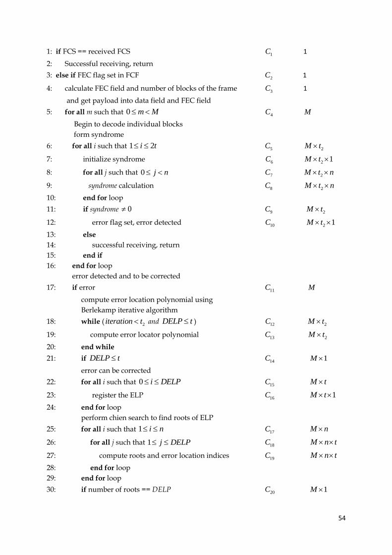
54

1: if FCS == received FCS 1C 1

2: Successful receiving, return

3: else if FEC flag set in FCF 2C 1

4: calculate FEC field and number of blocks of the frame 3C 1

and get payload into data field and FEC field

5: for all m such that 0 m M 4C M

Begin to decode individual blocks

form syndrome

6: for all i such that 1 2i t 5C 2M t

7: initialize syndrome 6C 2 1M t

8: for all j such that 0 j n 7C 2M t n

9: syndrome calculation 8C 2M t n

10: end for loop

11: if syndrome 0 9C 2M t

12: error flag set, error detected 10C 2 1M t

13: else

14: successful receiving, return

15: end if

16: end for loop

error detected and to be corrected

17: if error 11C M

compute error location polynomial using

Berlekamp iterative algorithm

18: while ( 2iteration t and DELP t ) 12C 2M t

19: compute error locator polynomial 13C 2M t

20: end while

21: if DELP t 14C 1M

error can be corrected

22: for all i such that 0 i DELP 15C M t

23: register the ELP 16C 1M t

24: end for loop

perform chien search to find roots of ELP

25: for all i such that 1 i n 17C M n

26: for all j such that 1 j DELP 18C M n t

27: compute roots and error location indices 19C M n t

28: end for loop

29: end for loop

30: if number of roots == DELP 20C 1M

55

31: for all i such that 0 i DELP 21C M t

received bits correspond to error location 22C 1M t

are complemented

32: else

33: uncorrectable error, receiving failed, return

34: end if

35: else

36: uncorrectable error detected, receiving failed, return

37: end if

38: else

39: successful receiving, return

40: end if

41: end for loop

42: else

43: receiving failed, return

44: end if

Total cost = 1 2 3 4 11 14 20 15 16 21 22C C C C C C C M C C C C M t

5 6 9 10 12 13 2 17C C C C C C M t C M n 18 19C C M n t

7 8C C M n t

The time complexity of the algorithm is given as 2O Mnt .

Time complexity RS encoder algorithm

Algorithm Cost Time

1: for all m such that 0 m M 1C M

begin to encode individual blocks

2: for all i such that 0 i n k 2C M n k

3: Initialize the output 3C 1M n k

4: end for loop

5: for all i such that 0k i 4C M k

6: feedback = index of input i XOR 1output n k 5C 1M k

7: if feedback 1 6C 1M k

8: for all j such that 0n k j 7C M k n k

9: the output is computed using- 8C 1M k n k

Generator polynomial

10: end for loop

11: else

12: output computed 9C 1M k

56

13: end if

14: end for loop

15: end for loop

The total cost is given by,

1 2 3 4 5 6 9 7 8C M C C M n k C C C C M k C C M k n k

Therefore, the time complexity of the RS encoder algorithm is O M k n k .

Time complexity of RS decoder algorithm

Algorithm Cost Time

1: if FCS == received FCS 1C 1

2: Successful receiving, return

3: else if FEC flag set in FCF 2C 1

4: calculate FEC field and number of blocks of the frame 3C 1

and get payload into data field and FEC field

5: for all m such that 0 m M 4C M

begin to decode individual blocks

syndrome detection

6: for all i such that 0 i n 5C M n

7: index the received data 6C 1M n

8: end for loop

9: for all i such that 1 i n k 7C M n k

10: syndrome initialized 8C 1M n k

11: for all j such that 0 j n 9C M n k n

12: syndrome computed 10C M n k n

13: end for loop

14: if syndrome 0 11C M n k

15: error flag set, error detected 12C 1M n k

16: else

17: successful receiving, return

18: end if

19: syndrome indexed 13C 1M n k

20: end for loop

21: if error detected, proceed error correction 14C M

compute error location polynomial Berlekamp

using iterative algorithm

23: initialize table entries and parameters 15C M

necessary to compute ELP

57

24: while ( iteration n k and DELP t ) 16C M n k

25: increment iteration 17C 1M n k

26: ELP computation continue 18C 1M n k

27: end while loop

28: iteration incremented 19C M

29: if DELP t , error can be corrected, proceed 20C M

30: for all i such that 1 i DELP 21C M t

31: ELP in index form 22C 1M t

32: end for loop

33: initialize counter for number of roots 23C M

34: for all i such that 1 i n 24C M n

35: compute and store the roots and 25C 1M n

error location number indices

36: end for loop

37: if counter == DELP, error can be corrected, 26C M

proceed

38: for all i such that 1 i DELP 27C M t

39: form polynomial for error values 28C 1M t

40: for all j such that 1 j i 29C M t t

41: form polynomial for error values 30C 1M t t

42: end for loop

43: index the polynomial form 31C 1M t

44: end for loop

evaluate errors at locations detected

45: for all i such that 0 i n 32C M n

46: convert received data to polynomial 33C 1M n

47: end for loop

48: for all i such that 0 i DELP 34C M t

49: for all j such that 1 j DELP 35C M t t

50: compute error and correct it 36C 1M t t

51: end for loop

52: end for loop

53: else

54: error cannot be corrected, receiving failed, return

55: end if

56: else

error cannot be corrected, receiving failed, return

57: end if

58

58: else

59: receiving failed, return

60: end if

61: end for loop

62: else

63: receiving failed, return

64: end if

Total cost of decoder algorithm is,

1 2 3 4 14 15 19 20 23 26C C C C C C C C C C M

21 22 27 28 31 34C C C C C C M t 2

29 30 35 36C C C C M t

5 6 24 25 32 33C C C C C C M n

7 8 11 12 13 16 17 18 9 10C C C C C C C C M n k C C M n k n

The time complexity of RS decoding algorithm is O M n k n .

The time requirements and complexities for a maximum message length of the block coding

algorithms are summarized in Table 10.

Table 10. Time complexity of block coding algorithms

Coding Schemes Encoding time complexity

Decoding error free time complexity

Decoding with max. error time complexity

Cyclic (15, 7) code O M k O M n 2O M n

Hamming (7, 4) code O M n k O M k n O M k n

Repetition (3, 1) code O M n O M n O M n

BCH (15, 5) code O M k n k 2O M t n 2O M t n

BCH (15, 7) code O M k n k 2O M t n 2O M t n

BCH (31, 21) code O M k n k 2O M t n 2O M t n

RS (15, 5) code O M k n k . O M n n k O M n k n

RS (15, 9) code O M k n k . O M n n k O M n k n

RS (15, 11) code O M k n k . O M n n k O M n k n

59

Analysis and Conclusions As mention in previous section, the successful packet transmission in IWSN is achieved by

strictly following the timing requirement (acknowledgement waiting time) from IEEE

802.15.4 standard and constrained memory resource of the embedded devices. The memory

footprint of block coding algorithms is shown in the Figures 19, 20, 21 and 22 with different

optimization options. The execution time is also shown in the Tables 6 - 9. We can notice

from the tables that, the encoding and decoding time are different due to different input

data. The decoding time without error and with maximum correctable error is also different

as the error bits introduced in the message significantly influence the processing time. The

decoding time without an error bit is much less than the decoding time with maximum error

because of the extra time required detecting the errors and correcting them. For our analysis

and conclusion of FEC algorithms, the measured execution time with high speed

optimization and memory consumption with high size optimization are taken in to

consideration. The results also show that the algorithms with the proposed optimization

options perform better than the other options.

Among the proposed block codes, BCH and RS algorithms with different parameters, such as

error correcting capability, block length, code rate and original message length are evaluated.

From Table 6, the execution times of RS (15, 11) and BCH (31, 21) are much faster than their

corresponding algorithms. That is, the performance of RS (15, 11) is better than RS (15, 9) and

RS (15, 5), but it has a relatively less error correcting capability. The same is true for BCH (31,

21) code, compared to BCH (15, 7) and BCH (15, 5) algorithms; its execution time is faster but

with small error correcting capability. The RS (15, 11) and BCH (31, 21) algorithms have

higher code rate and, therefore, are transmission efficient compare to their corresponding

candidates. From Figure 20, the RS (15, 11) code has less memory consumption than RS (15,

9) and RS (15, 5) codes. It is noticeable that for the same block length used, the algorithm

with high error correcting capability consumes larger memory and execution time. The BCH

(31, 21) requires large amount of memory compare to BCH (15, 5) and BCH (15, 7) codes due

to high block length. Therefore, BCH (31, 21) and RS (15, 11) codes perform better in terms of

processing time, memory and transmission efficiency from the proposed BCH and RS codes.

They are also selected for further comparison with the other proposed block codes, namely,

cyclic, hamming and repetition codes.

The classic cyclic (15, 7) code performs worst in processing time and memory consumption.

It takes 35 ms to decode a packet with maximum correctable error which is not feasible for

the timing requirement of the standard. It also requires huge amount of memory, almost 6K

bytes of RAM memory. The maximum RAM size for our platform is 8K bytes which is not

suitable to use it in memory limited embedded devices and impractical to apply in industrial

automation purpose. The cyclic (15, 7) has also less code rate relative to the other algorithms

and less error correcting capability. The repetition (3, 1) and hamming (7, 4) algorithms are

the second and third best candidates in terms of processing time, respectively. The memory

consumption of repetition (3, 1), nearly 5.6K bytes in RAM, is less compare to Hamming (7,

4) which requires almost 6K bytes of RAM memory. Repetition (3, 1) has higher error

correcting capability than hamming (7, 4). The drawback of repetition (3, 1) is; it has low

code rate compare to the other candidates which performs less in transmission efficiency.

60

BCH (31, 21), compare to Repetition (3, 1) and hamming (7, 4), has higher code rate but it has

slower processing time and require higher amount of memory.

Generally, RS (15, 11) is found to be the best candidate in terms of the memory it requires

and the execution time. RS (15, 11) has also the highest code rate and best error correcting

capability; it corrects 2 symbols in error out of 15 symbols. Since RS codes are multi-burst

error correcting codes, 8 consecutive bit errors can be corrected by applying RS (15, 11). The

transmission of data over a noisy wireless channel suffers from channel degradation, such as

burst errors. Therefore, the RS (15, 11) has a remarkable performance in wireless

communication compare to the other block codes.

The time complexity of decoding algorithms is evaluated in a worst case scenario analysis

and summarized in Table 10. The encoding and error free decoding time complexity of the

algorithms are also present in the table. It helps to compare and verify with the execution

time implemented in real time scenario. Some of the coding schemes are used for fair

comparison with the real implementation in the evaluation board. For example, cyclic (15, 7)

took a largest decoding time with maximum correctable errors compared to the other

schemes. The time complexity of cyclic (15, 7) code is also greater than the other schemes as

shown in Table 10. The RS (15, 11) code and repetition (3, 1) code have better performance in

time complexity compare to the other algorithms and verified with the real implementation.

In Hamming (7, 4) code and some of the BCH codes, namely, BCH (15, 7) and BCH (31, 21),

the encoding time is greater than the decoding time and can also be elaborated using the

complexity algorithm. From Hamming codes, the encoding complexity is approximately

28n k time unit and the decoding without error is 21n k n time unit which is

reasonable from the results but as it is optimized using high speed and balance optimization

levels, the encoding time is less than the decoding one. The BCH (15, 7, t = 2) has encoding

time complexity of roughly 56 time unit and decoding of 45 time unit. In case of BCH (31, 21,

t = 2), encoding complexity is 210 time unit and the decoding complexity is roughly 93 time

unit which has big difference and, therefore, the encoding time is appears to be greater than

the error free decoding time.

4.4.2 Evaluation Result of LDPC, Turbo and Block Codes

LDPC and Turbo codes are also considered to evaluate their performance in IWSNs. In this

section, the above FEC block codes are presented in addition to LDPC and Turbo codes for

evaluation and comparison purpose. The aim of this section is to evaluate the performance of

capacity approaching codes: LDPC and turbo codes in IWSNs and compare with the block

codes presented previously. For our analysis and discussion the performance of LDPC,

Turbo, Block codes and other coding schemes is presented in figure 23 for decoding bit error

rate of 410 . The figure indicates the bandwidth versus power efficiency of the coding

schemes and compares them with capacity bound. The performances of the FEC algorithms

are evaluated using none optimization, high speed optimization, high size optimization and

high balance optimization options. The memory consumption and processing time of LDPC

and Turbo coding algorithms for packet size ranged 5 to 70 bytes are also included in the

appendix.

61

Figure 23. FEC performance relative to capacity bound.

Processing Time Applying the same experimental setup described above, the processing time consumption of

FEC algorithms are listed in the Tables 11, 12, 13 and 14.

Table 11: Execution time of FEC with None Optimization

Error control coding schemes

Encoding time (ms) Decoding time with no error (ms)

Decoding time with max errors (ms)

Cyclic (15, 7) code

4.0433 ms 6.6600 ms 42.7667 ms

Hamming (7, 4) code

9.8116 ms 7.1633 ms 7.9333 ms

Repetition (3, 1) code

2.4267 ms 3.1967 ms 4.2467 ms

BCH (31, 21) code

8.9741 ms 3.3356 ms 9.4185 ms

RS (15, 11) code

1.6813 ms 2.4245 ms 4.9362 ms

LDPC (12, 4) code

30.4208 ms 68.7983 ms 95.0308 ms

TURBO (24, 8) code

11.1533 ms 10.3848 sec 10.4141 sec

62

Table 12: Execution time of FEC with High Speed Optimization

Error control coding schemes

Encoding time (ms) Decoding time with no error (ms)

Decoding time with max errors (ms)

Cyclic (15, 7) code

1.6333 ms 3.0067 ms 35.6833 ms

Hamming (7, 4) code

2.4500 ms 2.4908 ms 3.1383 ms

Repetition (3, 1) code

0.5133 ms 1.5167 ms 2.8000 ms

BCH (31, 21) code

2.4424 ms 1.7044 ms 4.4854 ms

RS (15, 11) code

0.5953 ms 0.9582 ms 2.3454 ms

LDPC (12, 4) code

2.3858 ms 25.4625 ms 37.1817 ms

TURBO (24, 8) code

1.9308 ms 0.7032 sec 0.7021 sec

Table 13: Execution time of FEC with High Size Optimization

Error control coding schemes

Encoding time (ms) Decoding time with no error (ms)

Decoding time with max errors (ms)

Cyclic (15, 7) code

2.3600 ms 7.4967 ms 33.7533 ms

Hamming (7, 4) code

6.4867 ms 5.6642 ms 6.1192 ms

Repetition (3, 1) code

1.7733 ms 2.3100 ms 3.2667 ms

BCH (31, 21) code

3.3356 ms 2.5099 ms 5.7825 ms

RS (15, 11) code

0.7665 ms 1.2323 ms 2.8047 ms

LDPC (12, 4) code

7.8750 ms 28.5717 ms 41.5683 ms

TURBO (24, 8) code

2.6950 ms 0.7369 sec 0.7393 sec

63

Table 14: Execution time of FEC with High Balance Optimization

Error control coding schemes

Encoding time (ms) Decoding time with no error (ms)

Decoding time with max errors (ms)

Cyclic (15, 7) code

1.7200 ms 3.3033 ms 35.9900 ms

Hamming (7, 4) code

2.5083 ms 2.6425 ms 3.2550 ms

Repetition (3, 1) code

0.7233 ms 1.6567 ms 2.8000 ms

BCH (31, 21) code

2.4547 ms 1.8675 ms 5.2121 ms

RS (15, 11) code

0.7502 ms 1.0947 ms 2.6942 ms

LDPC (12, 4) code

2.4617 ms 23.9692 ms 36.8025 ms

TURBO (24, 8) code

2.2633 ms 0.6972 sec 0.7048 sec

Memory Consumption

The memory consumption of LDPC and Turbo codes are measured and compared with the

block code algorithms that are evaluated in previous section as shown in Figures 24 – 27.

Figure 24. Footprint of FEC using None Optimization

64

Figure 25. Footprint of FEC using High Size Optimization

Figure 26. Footprint of FEC using High Speed Optimization

65

Figure 27. Footprint of FEC using High Balance Optimization

Time complexity of LDPC and Turbo codes

The time complexity of our LDPC and Turbo coding algorithms are presented as follows. Time complexity of Turbo encoder algorithm

Algorithm Cost Time

1: for all m such that 0 m M 1C M

begin to encode individual blocks

encoder#1

2: for all k such that 0 2k N 2C 2M N

Encoder#1 operates

3: Parity bits of first encoder generated 3C 2 1M N

4: end for loop

5: if 0state 4C 1M

6: Error has occured, could not terminate encoder#1

7: return

endif

permute data bits for encoder#2

8: for all k such that 0 k N 5C M N

9: data bits permuted 6C 1M N

10: end for loop

Encoder#2

66

11: for all k such that 0 k N 7C M N

12: encoder#2 operates

13: parity bits of second decoder generated 8C 1M N

14: end for loop

15: end for loop

The total cost of the algorithm is given by

Total cost = 1 2 3 42 2 1 1C M C M N C M N C M

5 6 7 81 1C M N C M N C M N C M N

The time complexity of the algorithm is represented by O MN .

Time complexity of Turbo decoder algorithm

Algorithm Cost Time

1: if FCS == received FCS 1C 1

2: Successful receiving, return

3: else if FEC flag set in FCF 2C 1

4: Calculate FEC field and number of blocks of the 3C 1

Frame and get payload into data field and FEC field

5: for all m such that 0 m M 4C M

Begin to decode individual blocks

6: for all k such that 0 k N 5C M N

zero apriori information for first

iteration of BCJR 6C 1M N

7: end for loop

8: for all iter such that 0 iter Niter 7C M Niter

9: modified BCJR algorithm (MAP decoder)

10: for all k such that 0 k N 8C M Niter N

for each trellis stage

11: for all n such that 0 n P 9C M Niter N P

12: for all i such that 0 2i 10C 2M Niter N P

13: map databit to PAM symbol 11C 2M Niter N P

14: map parity bit to PAM symbol 12C 2M Niter N P

15: compute parameter gamma using- 13C 2 ^ 2M Niter N P

exponential operation,

16: compute parameter gammae using- 14C 2 ^ 2M Niter N P

exponential operation

17: end for loop

18: end for loop

67

19: end for loop

calculate state alpha’s

20: initialize state 0 15C M Niter

21: for all n such that 0 n P 16C M Niter P

22: initialize alpha 17C 1M Niter P

23: end for loop

24: for all k such that 0 k N 18C M Niter N

25: total sum initialized 19C 1M Niter N

26: for all n such that 0 n P 20C M Niter N P

27: compute alpha 21C 1M Niter N P

28: compute total sum 22C 1M Niter N P

29: end for loop

30: for all n such that 0 n P 23C M Niter N P

31: normalize alpha 24C 1M Niter N P

32: end for loop

33: end for loop

calculate state beta’s

34: if trellis terminated 25C M Niter

35: final state is zero, first beta value set to 1 26C 1M Niter

36: other values set to zero

37: else

38: for all n such that 0 n P 27C M Niter P

39: beta values are equally likely 28C 1M Niter P

40: end for loop

41: end if

Iterate backwards through trellis

42: for all k such that 0N k 29C M Niter N

43: total sum initialized 30C 1M Niter N

44: for all n such that 0 n P 31C M Niter N P

45: compute beta 32C 1M Niter N P

46: compute total sum 33C 1M Niter N P

47: end for loop

48: for all n such that 0 n P 34C M Niter N P

49: normalize beta 35C 1M Niter N P

50: end for loop

51: end for loop

calculate extrinsic likelihood

52: for all k such that 0 k N 36C M Niter N

68

53: for all n such that 0 n P 37C M Niter N P

54: compute extrinsic components using- 38C 1M Niter N P

gammae and beta parameters

55: end for loop

56: calculate overall extrinsic likelihood- 39C log M Niter N

using logarithmic operation

57: end for loop

end modified BCJR algorithm

58: for all k such that 0 k N 40C M Niter N

59: Permute decoder#1 likelihoods to- 41C 1M Niter N

match decoder#2

60: end for loop

61: repeat modified BCJR algorithm cost and time of BCJR algorithm

62: for all k such that 0 k N 42C M Niter N

63: inverse permute decoder#2 likelihoods to- 43C 1M Niter N

match decoder#1

64: end for loop

65: end for loop

calculate overall likelihoods and then slice them

66: for all k such that 0 k N 44C M N

67: soft decision performed 45C 1M N

68: hard decision performed 46C 1M N

69: end for loop

70: end for loop

71: end if

The total cost of the algorithm is,

1 2 3 4 5 6 44 45 46 7 15 25 26

8 18 19 29 30 36 40 41 42 43

9 20 21 22 23 24 31 32 33 34 35 37 38

10 11 12

2

2 2

C C C C M C C C C C M N C C C C M Niter

C C C C C C C C C C M Niter N

C C C C C C C C C C C C C M Niter N P

C C C M Niter N P

13 14

16 17 27 28 15 25 26

8 18 19 29 30 36

2 2 ^ 2

2 2 log

C C M Niter N P

C C C C M Niter P M Niter N C C C M Niter

C C C C C C M Niter N

Therefore, the time complexity of this decoding algorithm is 2 ^ 2O M Niter N P

Time complexity of LDPC encoder algorithm

Algorithm Cost Time

1: for all m such that 0 m M 1C M

69

begin to encode individual blocks

2: for all i such that 0 i n 2C M n

3: Initialize the codeword variable 3C 1M n

4: for all j such that 0 j k 4C M n k

5: Encode using generator matrix 5C 1M n k

6: end for loop

7: end for loop

8: end for loop

The total cost is given by,

1 2 3 4 5C M C C M n C C M n k

The time complexity of LDPC encoding algorithm is O M n k .

Time complexity of LDPC decoder algorithm

In this algorithm, constant variables C and H for code node and check node sizes are used

respectively.

Algorithm Cost Time

1: if FCS == received FCS 1C 1

2: Successful receiving, return

3: else if FEC flag set in FCF 2C 1

4: Calculate FEC field and number of blocks of the frame 3C 1

And get payload into data field and FEC field

5: for all m such that 0 m M 4C M

Begin to decode individual blocks

6: for all i such that 0 i N 5C M N

Initialize the decoder codeword with received data 6C 1M N

7: end for loop

8: for all iter such that 0 iter Niter 7C M Niter

9: flag reset if the syndrome is all zero

10: for all i such that 0 i P 8C M Niter P

11: for all j such that 0 .j check node i size 9C M Niter P H

12: compute the parity check equations using- 10C 1M Niter P H

Received code word

13: end for loop

14: assign the value to .check node i syndrome 11C 1M Niter P

15: if . 1check node i syndrome 12C 1M Niter P

16: flag set 13C 1M Niter P

17: end if

70

18: end for loop

19: if (flag) 14C 1M Niter

20: for all i such that 0 i N 15C M Niter N

21: counter initialized 16C 1M Niter N

22: for all j such that 0 .j code node j size 17C M Niter N C

14: obtain .indexaux code node i j 18C 1M Niter N C

15: if .check node aux syndrome 19C 1M Niter N C

16: increment counter 20C 1M Niter N C

17: end if

17: end for loop

18: if counter threshold 21C 1M Niter N

19: bit at position i is flipped

20: end if

18: end for loop

19: else

20: flag reset, syndromes are all zero, return 22C 1M Niter

21: end if

22: end for loop

23: end for loop

24: end if

The total cost is given by

1 2 3 4 5 6 7 14 22 8 11 12 13

9 10 15 16 17 18 19 20

C C C C M C C M N C C C M Niter C C C C M Niter P

C C M Niter P H C C M Niter N C C C C M Niter N C

Therefore, the time complexity of the LDPC decoding algorithm is given by

O M Niter N C .

Analysis and Conclusions LDPC and Turbo codes are widely used FEC codes in the application of information coding

theory due to their capability of approaching Shannon capacity. It could be interesting to

evaluate them in IWSNs under circumstances where the execution time and limited memory

consumptions are important metrics to be strictly followed. For sake of our discussion and

conclusion, we focus on the processing time with high speed optimization and memory

consumption with high size optimization of LDPC (12, 4) and Turbo (24, 8) codes.

The decoding time of Turbo (24, 8) algorithm with maximum message length and correctable

errors is 0.7032 seconds as it can be seen in Table 11. It is not feasible to implement in IWSN

that incorporates the standard timing requirement. The execution time of LDPC (12, 4) code

is much faster than Turbo (24, 8) code, but it is far beyond the standard timing requirement

boundary. It also consumes huge amount of memory, nearly a size of 7K bytes in RAM.

71

Turbo (24, 8) code requires a lot of memory as it is shown in Figure 24, especially, in Read-

Only code memory compare to the rest of FEC candidates. Both Turbo and LDPC codes can

use considerably much longer block lengths in order to approach Shannon limit, however,

due to the memory constraint we are restricted to use shorter block length. According to the

results obtained, these two famous FEC codes are not suitable to be implemented in IWSN

with limited memory and processing time. Therefore, even though LDPC and Turbo codes

are close to capacity bound as shown in Figure 23, they fail to fulfill the requirements for

IWSN standard.

Generally, in our evaluation of FEC algorithms; RS (15, 11) is the first best candidate chosen

to be applied in IWSNs based on the performances from our results. It requires much less

memory nearly 1.2K bytes out of 6K bytes of RAM size. It takes 0.5953 ms to encode a

maximum packet size in the MAC layer and 0.9582 ms of decoding time without error or few

errors. For a worst case scenario, that is, when maximum correctable errors occurred, it takes

roughly 2.3 ms which is beyond the time limit requirement of the IEEE 802.15.4 standard in

IWSNs. However, this worst scenario happens when only maximum packet size of the

payload is transmitted which is applied rarely in real time and also happens when 13.3% of

the message is in error which again occurred very rare in practical applications.

One of the possible approaches to improve the performance in processing time and memory

of FEC algorithms is to use high performance IWSN-chip with high speed processor and

embedded memories (flash memory and SRAM). The High clock speed of the processor and

memory enhance the performance in processing time and memory consumption in order to

meet the necessary requirements of IWSNs. Another option is, to use hardware

implementation of FEC codes at the expense of hardware cost. The FEC code candidates with

less performance may also be further optimized to increase their feasibility in IWSN

implementation.

72

Chapter 5

Conclusions and Future Work

5.1 Summary and Conclusions

Reliability and latency are two important requirements we need to address within IWSNs in

industrial automation. It is a challenge to provide a deterministic real time communication

and reliable link due to the dynamic nature of wireless channels and harsh environment in

industrial wireless communication. Reliability is one of the primary requirements due to the

high probability of packet loss and transmission failure in wireless link. Therefore, IWSNs

apply a mechanism called ARQ in a MAC layer to provide reliable communication. ARQ

trigger an automatic packet retransmission whenever communication fails which results in

latency and network congestion. FEC code on MAC layer is another approach proposed to

mitigate latency. FEC code is used by introducing redundancy bits to recover corrupted data

due to noisy wireless channel at the expense of bandwidth.

In our project, the feasibility of FEC codes in IWSNs is realized based the timing requirement

of IEEE 802.15.4 based IWSN standard and limited memory of the embedded device. Several

FEC algorithms are proposed and evaluated with respect to the processing time and memory

consumption in IWSN chip with high performance core operating at 24MHz frequency. The

algorithms are applied on MAC layer without hardware support and interaction with radio

chip manufacturer. Our result shows that RS (15, 11) code is the best candidate chosen to be

suitable algorithm for IWSNs in industrial automation process in terms of processing time

and memory consumption. The other FEC candidates can also be feasible in IWSNs using the

chips with higher processor speed. One can also examine more suitable FEC code parameters

and optimize the FEC code implementations for higher efficiency. Moreover, the algorithms

can also be implemented using hardware implementation to improve their performance.

5.2 Future Work

In this thesis project, the evaluation and comparison of FEC coding algorithms on MAC layer

in IWSNs are implemented using pure C programming. The hardware implementation of

the FEC algorithms can be interesting to evaluate in IWSNs and see up to what extent the

performance has improved. The future work could be to implement our algorithms in real

industrial devices and harsh environment. Therefore, the performance of our solution can be

evaluated in real industrial environments and help strengthen our results.

Currently, reliable and robust routing protocol in WSNs is challenging topic and great deal

of research interest. Applying routing protocols on network layer play an important role to

improve the communication latency and reliable data transmission. The combination of FEC

schemes in MAC layer and robust routing protocols is also an interesting approach for

reliable and real time communication in IWSNs.

73

References

[1] ARM website: www.arm.com (Accessed 2013-03-30).

[2] Graham Wade. Signal Coding and Processing, Second Edition. Cambridge University Press

1994.

[3] Moon, Todd K. Error Correction Coding: Mathematical Methods and Algorithms. John Wiley

and Sons, Inc. 2005

[4] Franz Lemmermeyer. Error-correcting Codes.

[5] Robert H. Morelos-Zaragoza. The Art of Error Correcting Coding. 2002 John Wiley and

Sons Ltd.

[6] John G. Proakis, Masoud Salehi. Digital Communications, Fifth Edition, 2001.

[7] Chris Schmitt, Donny Hubener and Lamin Dumbuya. Cyclic Codes.

[8] STM32w108cb: www.st.com (Accessed 2013-04-10).

[9] STM32w108cb, STM32w108HB: High-Performance, 802.15.4 wireless system-on-chip.

[10] Kan Yu. On Reliable Real Time Communication in Industrial Wireless Sensor Networks.

Mälardalen University, 2012.

[11] J. Åkerberg, M. Gidlind, F.Reichenbach, and M. Björkman. Measurements on an

Industrial Wireless HART Network Supporting Profisafe: A case study. to appear in

IEEE Conference on Emerging Technologies and Factory Automation (ETFA'11), pages 1-8,

Sep. 2011.

[12] IEEE Standard for a Smart Transducer Interface for Sensors and Actuators Wireless

Communication Protocols and Transducer Electronic Data Sheet (TEDS) Formats. IEEE

Std 1451.5-2007, pages C1 - 236, Oct. 5, 2007.

[13] Hart 7 specification, http:www.hartcomm.org/, 2010 (Accessed 2013-06-10).

[14] Industrial Society of Automation, http://www.isa.org/ (Accessed 2013-02-10).

[15] Shenyang institute of automation, http://www.industrialwireless.cn/ (Accessed 2013- 03-20).

[16] IEEE Standard for Information Technology - telecommunications and information

exchange between systems - local and metropolitan area networks - specific

requirements part 15.4: Wireless Medium Access Control (MAC) and Physical Layer

(PHY) Specifications for Low Rate Wireless Personal Area Networks (WPANs). IEEE

Std 802.15.4 - 2006 (Revision of IEEE Std 802.15.4 - 2003), page 1 - 305, 2006.

[17] T. Lennvall, S. Svensson and F. Hekland. A Comparison of Wirelesshart and ZigBee for

Industrial Applications. In Factory Communication Systems, 2008. WFCS 2008. IEEE

International Workshop on, pages 85 - 88, may 2008.

74

[18] Vehbi C. Gungor, Member, IEEE, and Gerhard P. Hancke, Senior Member, IEEE.

Industrial Wireless Sensor Networks: Challenges, Design Principles, and Technical

Approaches.

[19] A. Sikora and V.F. Groza. Coexistence of IEEE 802.15.4 with other systems in the 2.4 GHz-

ISM-Band. Instrumentation and Measurement Technology Conference, 2005. IMTC

2005. Proceedings of the IEEE, IEEE 2005.

[20] P. Angskog, C. Karlsson, J.F Coll, J. Chilo and P. Stenumgaard. Source of Disturbances on

Wireless Communication in Industrial and Factor Environments.

[21] N. Sadeghi, S. Howard, S. Kasnavi, K. Iniewski, V.C. Gaudet and Schlegel. Analysis of

Error Control Code Use Ultra-Low-Power Wireless Sensor Networks. Circuits and Systems,

2006. ISCAS 2006. Proceedings. 2006 IEEE International Symposium.

[22] Y. Sankarasubramaniam, I. F. Akyildiz, S. W. McLaughlin. Energy efficiency based

packet size optimization in wireless sensor networks. In Sensor Network Protocols and

Applications, 2003. Proceedings of the First IEEE. 2003 IEEE International Workshop on, pages

1 - 8, 2003.

[23] A. Nandi, S. Kundu. Energy level performance of error control schemes in wireless

sensor networks. In Devices and Communications (ICDeCom), 2011 International Conference

on, page 1 - 5, 2011.

[24] M. Sartipi, F. Fekri. Source and channel coding in wireless sensor networks using LDPC

codes. In Sensor and Ad Hoc Communications and Networks, 2004. IEEE SECON 2004. 2004

First Annual IEEE Communications Society Conference on, page 309 - 316, 2004.

[25] G. Balakrishnan, M. Yang, Y. Jiang, Y. Kim. Performance analysis of error control codes

for wireless sensor networks. In Information Technology, 2007. ITNG'07. Fourth

International Conference on, page 876 - 879, 2007.

[26] E. R. Sanchez, F. Gandino, B. Montrucchio and M. Rebaudengo. Increasing effective

radiated power in wireless sensor networks with channel coding techniques. In

Electromagnetics in Advanced Applications, 2007. ICEAA 2007. Intenational Conference on,

pages 403 - 406, 2007.

[27] H. Karvonen and Carlos Pomalaza-Raez. A cross layer design of coding and awake/sleep periods in WSNs. In Personal, Indoor and Mobile Radio Communications, 2006 IEEE 17th International Symposium on, pages 1 - 5, 2006.

[28] Zhang Liankuan, Xiao Deqin, Tang Yi and Yang Zhang. Adaptive error control in

wireless sensor networks. IET, 2010.

[29] Oskar Eriksson, Erik Björnemo, Anders Ahlen and Mikael Gidlund. On hybrid ARQ

adaptive forward error correction in wireless sensor networks. In IECON 2011 - 37th

Annual Conference on IEEE Industrial Electronics Society, pages 3004 - 3010, 2011.

[30] CHEN Yan-ming, XU Yong-jun, WANG Qiu-guang and Xie Lei. An adaptive fault-

tolerant scheme for wireless sensor networks. In Communications and Mobile Computing,

75

2009. CMC'09. WRI International Conference on, pages 32 - 36, 2009.

[31] Youssef Charfi, Naoki Wakamiya and Masayuki Murata. Adaptive and reliable multi-

path transmission in wireless sensor networks using forward error correction and

feedback. In Wireless Communications and Networking Conference, 2007. WCNC 2007.

IEEE, pages 3681 - 3686, 2007.

[32] Zhiqiang Xiong, Zongkai Yang, Wei Liu and Zhen Feng. A lightweight FEC algorithm

for fault tolerant routing in wireless sensor networks. In Wireless Communications,

Networking and Mobile Computing, 2006. WiCOM 2006. International Conference on, pages

1 - 4, September 2006.

[33] Sukun Kim, Rodrigo Fonseca and David Culler. Reliable transfer on wireless sensor

networks. In Sensor and Ad Hoc Communications and Networks, 2004. IEEE SECON

2004. 2004 First Annual IEEE Communications Society Conference on, pages 449 - 459, Oct.

2004.

[34] Kan Yu, Filip Barac, Mikael Gidlund, Johan Åkerberg and Mats Björkman. A flexible

error correction scheme for IEEE 802.15.4-based industrial wireless sensor networks. In

Industrial Electronics (ISIE), 2012 IEEE International Symposium on, pages 1172 - 1177,

2012.

[35] Filip Barac, Kan Yu, Mikael Gidlund, Johan Åkerberg and Mats Björkman. Towards

reliable and lightweight communication in industrial wireless sensor networks. In

Industrial Informatics (INDIN), 2012 10th IEEE International Conference on, pages 1218 -

1224, 2012.

[36] Eytan Modiano. Communication Systems Engineering. MIT Open Course Ware.

[37] Franz Lemmermeyer. Error-correcting Codes. February 16, 2005.

[38] John G. Proakis, Masoud Salehi. Communication Systems Engineering, Second Edition.

by Prentice-Hall, Inc. Upper Saddle River, New Jersey, 2002.

[39] Priti Shankar. Error Correcting Codes. Resonance, pages 33 - 47, 1997.

[40] Matteo Petracca, Marco Ghibaudi, Claudio Salvadori, Paolo Pagano and Daniele

Munatetto. In Computers and Communications (ISCC), 2011 IEEE Symposium on, Pages 43

- 48, 2011.

[41] Vahid Meghadadi. Cyclic Codes. February 2008.

[42] I. S. Reed, G. Solomon. Polynomial Codes Over Certain Finite Fields. In Journal of the Society for Industrial and Applied Mathematics, Vol. 8, No. 2 (June 1960), pages 300 - 304.

[43] Saurabh Mahajan, Gurpadam Singh. BER Performance of Reed-Solomon Code using M-

ary FSK Modulation in AWGN Channel. In International Journal of Advances in Science

and Technology, 2011.

76

[44] Wen Xu. Implementation and Performance Evaluation of Reed-Solomon Codes. School

of Electrical and Computer Engineering, Cornell University.

[45] Sarah J. Johnson. Introducing Low-Density Parity-Check Codes. School of Electrical

Engineering and Computer Science, The University of Newcastle, Australia.

[46] William E. Ryan. A turbo code tutorial. New Mexico State University, Box, Volume 30001,

pages 3 - 0, 1997.

[47] Dong Yang, Mikael Gidlund, Wei Shen, Youzhi Xu, Tingting Zhang, Hongke Zhang.

CCA- Embedded TDMA enabling acyclic traffic in industrial wireless sensor networks.

In Ad Hoc Networks, 2012.

[48] I. F. Akyildiz, W. Su, Y. Sankarasubramaniam, E. Cayirci. Wireless sensor networks: a

survey. In Computer Networks, Volume 38, pages 393 - 422, 2002.

[49] Jon T. Adams. An introduction to IEEE STD 802.15.4. In Aerospace Conference, 2006 IEEE,

pages 8 - pp, 2006.

[50] Jose A. Gutierrez, Marco Naeve, Ed Callaway, Monique Bourgeois, Vinay Mitter and

Bob Heile. IEEE 802.15.4: a Developing standard for low-power low-cost wireless

personal area networks. In Network, IEEE, volume 15, pages 12 - 19, 2001.

[51] Jianliang Zheng, Myung J. Lee. A comprehensive performance study of IEEE 802.15.4.

IEEE Press Book Los Alamitos, 2004.

[52] Pouria Zand, Supriyo Chatterjea, Kallol Das and Paul Havinga. Wireless industrial

monitoring and control networks: the journey so far and the road ahead. In Journal of

Sensor and Actuator Networks 1, pages 123 - 152, 2012.

[53] Johan Åkerberg, Mikael Gidlund and Mats Björkman. Future research challenges in

wireless sensor and actuator networks targeting industrial automation. In Industrial

Informatics (INDIN), 2011 9th IEEE International Conference on, pages 410 - 415, 2011.

[54] S. Microelectronics. STM32W-SK and STM32W-EXT starter and extension kits for

STM32W108xx Microcontrollers. [online], 2012.

[55] Liming Xu, Jingqi Fu. The design and implementation of industrial monitoring wireless

sensor networks based on improved TDMA MAC protocol. In Control and Decision

Conference (CCDC), 2012 24th chinese, pages 3358 - 3362, 2012.

[56] Sunghyun Choi, Youngkyu Choi, Inkyu Lee. IEEE 802.11 MAC-Level FEC scheme with

retransmission combining. In Wireless Communications, IEEE Transactions on, pages 203 -

211, 2006.

[57] J. Lin, K. Feng, Y. Huang and L. Wang. Novel design and analysis of aggregated ARQ

protocols for IEEE 802.11n networks. IEEE, 2013.

[58] Zhao Cheng, Mark Perillo and Wendi B. Heinzelman. General network lifetime and cost

models for evaluating sensor network deployment strategies. In Mobile Computing, IEEE

77

Transactions on, Pages 484 - 497, 2008.

[59] Sarah J. Johnson. Introduction to Low-Density Parity-Check Codes. School of Electrical

Engineering and Computer Science, The University of Newcastle, Australia.

[60] Author: VA. Turbo Code Primer. July 4, 2005, http://www.vashe.org.

[61] Adams, Jon T. An introduction to IEEE STD 802.15.4. Aerospace Conference, 2006 IEEE.

IEEE, 2006.

[62] Daniel J. Costello, Jr. The Genesis of Coding Theory. Coding Research Group,

Department of Electrical Engineering, University of Notre Dame, Notre Dame, IN

46556, 2009 School of Information Theory, Northwestern University, August 10, 2009.

[63] Bono Favio, Renaldi Graziano. Analysis of current and potential sensor network

technologies and their incorporation as embedded structural system. EUR - Scientific

and Technical Research Reports, Publications office of the European Union 2013.

78

Appendix

Table 14. Execution time of Cyclic (15, 7) code with None Optimization

Packet size[bytes] Encoding time (ms) Decoding time with no error (ms)

Decoding time with max Errors (ms)

20 1.1625 1.9148 12.2954

30 1.7690 2.9138 18.7104

40 2.3249 3.8295 24.5908

50 2.9314 4.8285 31.0058

60 3.4874 5.7443 36.8862

70 4.0433 6.6600 42.7667

Table 15. Execution time of Cyclic (15, 7) code with High Speed Optimization

Packet size[bytes] Encoding time (ms) Decoding time with no error (ms)

Decoding time with max Errors (ms)

20 0.4696 0.8644 10.2590

30 0.7146 1.3154 15.6115

40 0.9392 1.7288 20.5179

50 1.1842 2.1798 25.8704

60 1.4088 2.5933 30.7769

70 1.6333 3.0067 35.6833

Table 16. Execution time of Cyclic (15, 7) code with High Balance Optimization

Packet size[bytes] Encoding time (ms) Decoding time with no error (ms)

Decoding time with max Errors (ms)

20 0.4945 0.9497 10.3471

30 0.7525 1.4452 15.7456

40 0.9890 1.8994 20.6943

50 1.2470 2.3949 26.0928

60 1.4835 2.8491 31.0414

70 1.7200 3.3033 35.9900

Table 17. Execution time of Cyclic (15, 7) code with High Balance Optimization

Packet size[bytes] Encoding time (ms) Decoding time with no error (ms)

Decoding time with max Errors (ms)

20 0.6785 2.1553 9.7041

30 1.0325 3.2798 14.7671

40 1.3570 4.3106 19.4082

50 1.7110 5.4351 24.4712

60 2.0355 6.4659 29.1123

70 2.3600 7.4967 33.7533

79

Table 18. Execution time of Hamming (7, 4) code with no compiler Optimization

Packet size[bytes] Encoding time (ms) Decoding time with no error (ms)

Decoding time with max Errors (ms)

20 2.8033 2.0467 2.2667

30 4.2050 3.0700 3.4000

40 5.6066 4.0933 4.5333

50 7.0083 5.1167 5.6667

60 8.4100 6.1400 6.8000

70 9.8116 7.1633 7.9333

Table 19. Execution time of Hamming (7, 4) code with High Speed Optimization

Packet size[bytes] Encoding time (ms) Decoding time with no error (ms)

Decoding time with max Errors (ms)

20 0.7000 0.7117 0.8967

30 1.0500 1.0675 1.3450

40 1.4000 1.4233 1.7933

50 1.7500 1.7792 2.2417

60 2.1000 2.1350 2.6900

70 2.4500 2.4908 3.1383

Table 20. Execution time of Hamming (7, 4) code with High Balance Optimization

Packet size[bytes] Encoding time (ms) Decoding time with no error (ms)

Decoding time with max Errors (ms)

20 0.7167 0.7550 0.9300

30 1.0750 1.1325 1.3950

40 1.4333 1.5100 1.8600

50 1.7917 1.8875 2.3250

60 2.1500 2.2650 2.7900

70 2.5083 2.6425 3.2550

Table 21. Execution time of Hamming (7, 4) code with High Size Optimization

Packet size[bytes] Encoding time (ms) Decoding time with no error (ms)

Decoding time with max Errors (ms)

20 1.8533 1.6183 1.7483

30 2.7800 2.4275 2.6225

40 3.7067 3.2367 3.4967

50 4.6333 4.0458 4.3708

60 5.5600 4.8550 5.2450

70 6.4867 5.6642 6.1192

80

Table 22. Execution time of Repetition (3, 1) code with None Optimization

Packet size[bytes] Encoding time (ms) Decoding time with no error (ms)

Decoding time with max Errors (ms)

20 0.6933 0.9133 1.2133

30 1.0400 1.3700 1.8200

40 1.3867 1.8267 2.4267

50 1.7333 2.2833 3.0333

60 2.0800 2.7400 3.6400

70 2.4267 3.1967 4.2467

Table 23. Execution time of Repetition (3, 1) code with High Speed Optimization

Packet size[bytes] Encoding time (ms) Decoding time with no error (ms)

Decoding time with max Errors (ms)

20 0.1467 0.4333 0.8000

30 0.2200 0.6500 1.2000

40 0.2933 0.8667 1.6000

50 0.3667 1.0833 2.0000

60 0.4400 1.3000 2.4000

70 0.5133 1.5167 2.8000

Table 24. Execution time of Repetition (3, 1) code with High Balance Optimization

Packet size[bytes] Encoding time (ms) Decoding time with no error (ms)

Decoding time with max Errors (ms)

20 0.2067 0.4733 0.8000

30 0.3100 0.7100 1.2000

40 0.4133 0.9467 1.6000

50 0.5167 1.1833 2.0000

60 0.6200 1.4200 2.4000

70 0.7233 1.6567 2.8000

Table 25. Execution time of Repetition (3, 1) code with High Size Optimization

Packet size[bytes] Encoding time (ms) [ms]

Decoding time with no error[ms]

Decoding time with max Errors[ms]

20 0.5067 0.6600 0.9333

30 0.7600 0.9900 1.4000

40 1.0133 1.3200 1.8667

50 1.2667 1.6500 2.3333

60 1.5200 1.9800 2.8000

70 1.7733 2.3100 3.2667

81

Table 26. Execution time of BCH (15, 5) code with High speed Optimization

Packet size[bytes] Encoding time (ms) Decoding time with no error (ms)

Decoding time with max Errors (ms)

20 0.5720 1.6867 4.8293

30 0.8580 2.5300 7.2440

40 1.1440 3.3733 9.6587

50 1.4300 4.2167 12.0733

60 1.7160 5.0600 14.4880

70 2.0020 5.9033 16.9027

Table 27. Execution time of BCH (15, 5) code with High Balance Optimization

Packet size[bytes] Encoding time (ms) Decoding time with no error (ms)

Decoding time with max Errors (ms)

20 0.6067 2.0613 5.4347

30 0.9100 3.0920 8.1520

40 1.2133 4.1227 10.8693

50 1.5167 5.1533 13.5867

60 1.8200 6.1840 16.3040

70 2.1233 7.2147 19.0213

Table 28. Execution time of BCH (15, 5) code with High Size Optimization

Packet size[bytes] Encoding time (ms) Decoding time with no error (ms)

Decoding time with max Errors (ms)

20 1.0653 3.2360 6.0013

30 1.5980 4.8540 9.0020

40 2.1307 6.4720 12.0027

50 2.6633 8.0900 15.0033

60 3.1960 9.7080 18.0040

70 3.7287 11.3260 21.0047

Table 29. Execution time of BCH (15, 5) code with None Optimization

Packet size[bytes] Encoding time (ms) Decoding time with no error (ms)

Decoding time with max Errors (ms)

20 2.3520 3.9987 10.6533

30 3.5280 5.9980 15.9800

40 4.7040 7.9973 21.3067

50 5.8800 9.9967 26.6333

60 7.0560 11.9960 31.9600

70 8.2320 13.9953 37.2867

82

Table 30. Execution time of BCH (15, 7) code with High Speed Optimization

Packet size[bytes] Encoding time (ms) Decoding time with no error (ms)

Decoding time with max Errors (ms)

20 0.4207 0.8146 2.3364

30 0.6402 1.2396 3.5554

40 0.8414 1.6292 4.6728

50 1.0609 2.0542 5.8918

60 1.2621 2.4438 7.0092

70 1.4633 2.8333 8.1267

Table 31. Execution time of BCH (15, 7) code with High Size Optimization

Packet size[bytes] Encoding time (ms) Decoding time with no error (ms)

Decoding time with max Errors (ms)

20 0.9152 1.0935 2.6306

30 1.3927 1.6640 4.0031

40 1.8304 2.1869 5.2613

50 2.3079 2.7574 6.6338

60 2.7456 3.2804 7.8919

70 3.1833 3.8033 9.1500

Table 32. Execution time of BCH (15, 7) code with High Balance Optimization

Packet size[bytes] Encoding time (ms) Decoding time with no error (ms)

Decoding time with max Errors (ms)

20 0.4600 0.7916 2.4898

30 0.7000 1.2046 3.7887

40 0.9200 1.5832 4.9795

50 1.1600 1.9962 6.2785

60 1.3800 2.3747 7.4693

70 1.6000 2.7533 8.6600

Table 33. Execution time of BCH (15, 7) code with None Optimization

Packet size[bytes] Encoding time (ms) Decoding time with no error (ms)

Decoding time with max Errors (ms)

20 2.0403 1.5439 4.6642

30 3.1048 2.3494 7.0977

40 4.0806 3.0878 9.3284

50 5.1451 3.8933 11.7619

60 6.1209 4.6316 13.9926

70 7.0967 5.3700 16.2233

83

Table 34. Execution time of BCH (31, 21) code with High Speed Optimization

Packet size[bytes] Encoding time (ms) Decoding time with no error (ms)

Decoding time with max Errors (ms)

20 0.7237 0.5050 1.3290

30 1.0855 0.7575 1.9935

40 1.4473 1.0100 2.6580

50 1.8092 1.2625 3.3225

60 2.0805 1.4519 3.8209

70 2.4424 1.7044 4.4854

Table 35. Execution time of BCH (31, 21) code with High Size Optimization

Packet size[bytes] Encoding time (ms) Decoding time with no error (ms)

Decoding time with max Errors (ms)

20 0.9883 0.7437 1.7133

30 1.4825 1.1155 2.5700

40 1.9767 1.4873 3.4267

50 2.4708 1.8592 4.2833

60 2.8415 2.1380 4.9258

70 3.3356 2.5099 5.7825

Table 36. Execution time of BCH (31, 21) code with High Balance Optimization

Packet size[bytes] Encoding time (ms) Decoding time with no error (ms)

Decoding time with max Errors (ms)

20 0.7273 0.5533 1.5443

30 1.0910 0.8300 2.3165

40 1.4547 1.1067 3.0887

50 1.8183 1.3833 3.8608

60 2.0911 1.5908 4.4400

70 2.4547 1.8675 5.2121

Table 37. Execution time of BCH (31, 21) code with None Optimization

Packet size[bytes] Encoding time (ms) Decoding time with no error (ms)

Decoding time with max Errors (ms)

20 2.6590 0.9883 2.7907

30 3.9885 1.4825 4.1860

40 5.3180 1.9767 5.5813

50 6.6475 2.4708 6.9767

60 7.6446 2.8415 8.0232

70 8.9741 3.3356 9.4185

84

Table 38. Execution time of RS (15, 5) code with High Speed Optimization

Packet size[bytes] Encoding time (ms) Decoding time with no error (ms)

Decoding time with max Errors (ms)

20 0.4077 1.3150 3.9990

30 0.6115 1.9725 5.9985

40 0.8153 2.6300 7.9980

50 1.0192 3.2875 9.9975

60 1.2230 3.9450 11.9970

70 1.4268 4.6025 13.9965

Table 39. Execution time of RS (15, 5) code with High Size Optimization

Packet size[bytes] Encoding time (ms) Decoding time with no error (ms)

Decoding time with max Errors (ms)

20 0.5290 1.7093 4.7783

30 0.7935 2.5640 7.1675

40 1.0580 3.4187 9.5567

50 1.3225 4.2733 11.9458

60 1.5870 5.1280 14.3350

70 1.8515 5.9827 16.7242

Table 40. Execution time of RS (15, 5) code with High Balance Optimization

Packet size[bytes] Encoding time (ms) Decoding time with no error (ms)

Decoding time with max Errors (ms)

20 0.5350 1.6983 4.9647

30 0.8025 2.5475 7.4470

40 1.0700 3.3967 9.9293

50 1.3375 4.2458 12.4117

60 1.6050 5.0950 14.8940

70 1.8725 5.9442 17.3763

Table 41. Execution time of RS (15, 5) code with None Optimization

Packet size[bytes] Encoding time (ms) Decoding time with no error (ms)

Decoding time with max Errors (ms)

20 1.2080 3.0970 8.7720

30 1.8120 4.6455 13.1580

40 2.4160 6.1940 17.5440

50 3.0200 7.7425 21.9300

60 3.6240 9.2910 26.3160

70 4.2280 10.8395 30.7020

85

Table 42. Execution time of RS (15, 9) code with High Speed Optimization

Packet size[bytes] Encoding time (ms) Decoding time with no error (ms)

Decoding time with max Errors (ms)

20 0.1979 0.5069 1.3683

30 0.2771 0.7096 1.9157

40 0.3562 0.9124 2.4630

50 0.4354 1.1151 3.0103

60 0.5542 1.4192 3.8313

70 0.6333 1.6220 4.3787

Table 43. Execution time of RS (15, 9) code with High Size Optimization

Packet size[bytes] Encoding time (ms) Decoding time with no error (ms)

Decoding time with max Errors (ms)

20 0.2950 0.6298 1.5417

30 0.4130 0.8817 2.1583

40 0.5310 1.1336 2.7750

50 0.6490 1.3855 3.3917

60 0.8260 1.7634 4.3167

70 0.9440 2.0153 4.9333

Table 44. Execution time of RS (15, 9) code with High Balance Optimization

Packet size[bytes] Encoding time (ms) Decoding time with no error (ms)

Decoding time with max Errors (ms)

20 0.2712 0.6079 1.5892

30 0.3797 0.8511 2.2248

40 0.4882 1.0942 2.8605

50 0.5968 1.3374 3.4962

60 0.7595 1.7022 4.4497

70 0.8680 1.9453 5.0853

Table 45. Execution time of RS (15, 9) code with None Optimization

Packet size[bytes] Encoding time (ms) Decoding time with no error (ms)

Decoding time with max Errors (ms)

20 0.6754 1.1908 2.9075

30 0.9456 1.6672 4.0705

40 1.2157 2.1435 5.2335

50 1.4859 2.6198 6.3965

60 1.8911 3.3343 8.1410

70 2.1613 3.8107 9.3040

86

Table 46. Execution time of RS (15, 11) code with High Speed Optimization

Packet size[bytes] Encoding time (ms) Decoding time with no error (ms)

Decoding time with max Errors (ms)

20 0.1832 0.2948 0.7217

30 0.2747 0.4422 1.0825

40 0.3663 0.5897 1.4433

50 0.4579 0.7371 1.8042

60 0.5037 0.8108 1.9846

70 0.5953 0.9582 2.3454

Table 47. Execution time of RS (15, 11) code with High Size Optimization

Packet size[bytes] Encoding time (ms) Decoding time with no error (ms)

Decoding time with max Errors (ms)

20 0.2358 0.3792 0.8630

30 0.3538 0.5687 1.2945

40 0.4717 0.7583 1.7260

50 0.5896 0.9479 2.1575

60 0.6485 1.0427 2.3733

70 0.7665 1.2323 2.8047

Table 48. Execution time of RS (15, 11) code with High Balance Optimization

Packet size[bytes] Encoding time (ms) Decoding time with no error (ms)

Decoding time with max Errors (ms)

20 0.2308 0.3368 0.8290

30 0.3463 0.5053 1.2435

40 0.4617 0.6737 1.6580

50 0.5771 0.8421 2.0725

60 0.6348 0.9263 2.2797

70 0.7502 1.0947 2.6942

Table 49. Execution time of RS (15, 11) code with None Optimization

Packet size[bytes] Encoding time (ms) Decoding time with no error (ms)

Decoding time with max Errors (ms)

20 0.5173 0.7460 1.5188

30 0.7760 1.1190 2.2782

40 1.0347 1.4920 3.0377

50 1.2933 1.8650 3.7971

60 1.4227 2.0515 4.1768

70 1.6813 2.4245 4.9362

87

Table 50. Execution time of LDPC (12, 4) code

Packet size[bytes] Encoding time (ms) Decoding time with no error (ms)

Decoding time with max Errors (ms)

20 8.6917 19.6567 27.1517

30 13.0375 29.4850 40.7275

40 17.3833 39.3133 54.3033

50 21.7292 49.1417 67.8792

60 26.0750 58.9700 81.4550

70 30.4208 68.7983 95.0308

Table 51. Execution time of LDPC (12, 4) code with High Speed Optimization

Packet size[bytes] Encoding time (ms) Decoding time with no error (ms)

Decoding time with max Errors (ms)

20 0.6817 7.2750 10.6233

30 1.0225 10.9125 15.9350

40 1.3633 14.5500 21.2467

50 1.7042 18.1875 26.5583

60 2.0450 21.8250 31.8700

70 2.3858 25.4625 37.1817

Table 52. Execution time of LDPC (12, 4) code with High Balance Optimization

Packet size[bytes] Encoding time (ms) Decoding time with no error (ms)

Decoding time with max Errors (ms)

20 0.7033 6.8483 10.5150

30 1.0550 10.2725 15.7725

40 1.4067 13.6967 21.0300

50 1.7583 17.1208 26.2875

60 2.1100 20.5450 31.5450

70 2.4617 23.9692 36.8025

Table 53. Execution time of LDPC (12, 4) code with High Size Optimization

Packet size[bytes] Encoding time (ms) Decoding time with no error (ms)

Decoding time with max Errors (ms)

20 2.2500 8.1633 11.8767

30 3.3750 12.2450 17.8150

40 4.5000 16.3267 23.7533

50 5.6250 20.4083 29.6917

60 6.7500 24.4900 35.6300

70 7.8750 28.5717 41.5683

88

Table 54. Execution time of Turbo code, rate 1/3 with no optimization

Packet size[bytes] Encoding time (ms) Decoding time with no error (ms)

Decoding time with max Errors (ms)

20 3.1867 ms 2.9671 sec 2.9755 sec

30 4.7800 ms 4.4506 sec 4.4632 sec

40 6.3733 ms 5.9342 sec 5.9509 sec

50 7.9667 ms 7.4177 sec 7.4386 sec

60 9.5600 ms 8.9013 sec 8.9264 sec

70 11.1533 ms 10.3848 sec 10.4141 sec

Table 55. Execution time of Turbo code, rate 1/3 with High Speed Optimization

Packet size[bytes] Encoding time (ms) Decoding time with no error (ms)

Decoding time with max Errors (ms)

20 0.5517 ms 0.2009 sec 0.2006 sec

30 0.8275 ms 0.3014 sec 0.3009 sec

40 1.1033 ms 0.4018 sec 0.4012 sec

50 1.3792 ms 0.5023 sec 0.5015 sec

60 1.6550 ms 0.6028 sec 0.6018 sec

70 1.9308 ms 0.7032 sec 0.7021 sec

Table 56. Execution time of Turbo code, rate 1/3 with High Balance Optimization

Packet size[bytes] Encoding time (ms) Decoding time with no error (ms)

Decoding time with max Errors (ms)

20 0.6467 ms 0.1992 sec 0.2014 sec

30 0.9700 ms 0.2988 sec 0.3020 sec

40 1.2933 ms 0.3984 sec 0.4027 sec

50 1.6167 ms 0.4980 sec 0.5034 sec

60 1.9400 ms 0.5976 sec 0.6041 sec

70 2.2633 ms 0.6972 sec 0.7048 sec

Table 57. Execution time of Turbo code, rate 1/3 with High Size Optimization

Packet size[bytes] Encoding time (ms) Decoding time with no error (ms)

Decoding time with max Errors (ms)

20 0.7700 ms 0.2106 sec 0.2112 sec

30 1.1550 ms 0.3158 sec 0.3168 sec

40 1.5400 ms 0.4211 sec 0.4225 sec

50 1.9250 ms 0.5264 sec 0.5281 sec

60 2.3100 ms 0.6317 sec 0.6337 sec

70 2.6950 ms 0.7369 sec 0.7393 sec

89

Table 58. Footprint of Cyclic (15, 7) code

Packet size[byte]

Memory type None High size optimization

High speed optimization

High balance optimization

20

RO code memory (Bytes)

4992 3216 3800 3412

RO data memory (Bytes)

368 47 66 47

RW data memory (Bytes)

2768 2768 2768 2768

30

RO code memory (Bytes)

4992 3216 3800 3412

RO data memory (Bytes)

368 57 76 57

RW data memory (Bytes)

3440 3440 3440 3440

40

RO code memory (Bytes)

4992 3220 3812 3416

RO data memory (Bytes)

368 67 84 67

RW data memory (Bytes)

4056 4056 4056 4056

50

RO code memory (Bytes)

4992 3220 3808 3416

RO data memory (Bytes)

368 77 96 77

RW data memory (Bytes)

4728 4728 4728 4728

60

RO code memory (Bytes)

4996 3220 3804 3416

RO data memory (Bytes)

368 87 106 87

RW data memory (Bytes)

5344 5344 5344 5344

70

RO code memory (Bytes)

4992 3216 3800 3420

RO data memory (Bytes)

368 97 114 97

RW data memory (Bytes)

5960 5960 5960 5960

90

Table 59. Footprint Hamming (7, 4) code

Packet size[byte]

Memory type None High size optimization

High speed optimization

High balance optimization

20

RO code memory (Bytes)

1944 1336 1648 1472

RO data memory (Bytes)

344 138 144 138

RW data memory (Bytes)

1744 1744 1744 1744

30

RO code memory (Bytes)

1944 1336 1648 1472

RO data memory (Bytes)

344 142 154 142

RW data memory (Bytes)

2384 2384 2384 2384

40

RO code memory (Bytes)

1948 1340 1652 1480

RO data memory (Bytes)

344 148 164 148

RW data memory (Bytes)

3024 3024 3024 3024

50

RO code memory (Bytes)

1948 1340 1652 1480

RO data memory (Bytes)

344 152 174 152

RW data memory (Bytes)

3664 3664 3664 3664

60

RO code memory (Bytes)

1948 1340 1648 1480

RO data memory (Bytes)

344 158 183 158

RW data memory (Bytes)

4304 4304 4304 4304

70

RO code memory (Bytes)

1948 1340 1644 1480

RO data memory (Bytes)

344 162 196 162

RW data memory (Bytes)

4944 4944 4944 4944

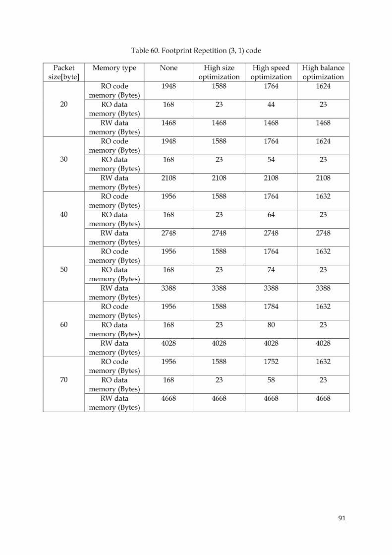
91

Table 60. Footprint Repetition (3, 1) code

Packet size[byte]

Memory type None High size optimization

High speed optimization

High balance optimization

20

RO code memory (Bytes)

1948 1588 1764 1624

RO data memory (Bytes)

168 23 44 23

RW data memory (Bytes)

1468 1468 1468 1468

30

RO code memory (Bytes)

1948 1588 1764 1624

RO data memory (Bytes)

168 23 54 23

RW data memory (Bytes)

2108 2108 2108 2108

40

RO code memory (Bytes)

1956 1588 1764 1632

RO data memory (Bytes)

168 23 64 23

RW data memory (Bytes)

2748 2748 2748 2748

50

RO code memory (Bytes)

1956 1588 1764 1632

RO data memory (Bytes)

168 23 74 23

RW data memory (Bytes)

3388 3388 3388 3388

60

RO code memory (Bytes)

1956 1588 1784 1632

RO data memory (Bytes)

168 23 80 23

RW data memory (Bytes)

4028 4028 4028 4028

70

RO code memory (Bytes)

1956 1588 1752 1632

RO data memory (Bytes)

168 23 58 23

RW data memory (Bytes)

4668 4668 4668 4668

92

Table 61. Footprint of BCH (15, 5) code

Packet size[byte]

Memory type None High size optimization

High speed optimization

High balance optimization

20

RO code memory (Bytes)

2996 2124 2972 2364

RO data memory (Bytes)

412 183 184 183

RW data memory (Bytes)

1876

1876 1876 1876

30

RO code memory (Bytes)

2996 2124 2972 2364

RO data memory (Bytes)

412 193 194 193

RW data memory (Bytes)

2516 2516 2516 2516

40

RO code memory (Bytes)

3004 2128 2976 2368

RO data memory (Bytes)

412 203 204 203

RW data memory (Bytes)

3156 3156 3156 3156

50

RO code memory (Bytes)

3004 2128 2976 2368

RO data memory (Bytes)

412 213 214 213

RW data memory (Bytes)

3796 3796 3796 3796

60

RO code memory (Bytes)

3004 2128 2972 2368

RO data memory (Bytes)

412 223 224 223

RW data memory (Bytes)

4436 4436 4436 4436

70

RO code memory (Bytes)

3004 2128 2972 2368

RO data memory (Bytes)

412 233 234 233

RW data memory (Bytes)

5076 5076 5076 5076

93

Table 62. Memory footprint of different BCH codes

BCH codes

Memory Types None High Size Optimization

High Balance Optimization

High Speed Optimization

BCH (15,5) RO code memory (Bytes)

3028 2120 2368 2972

RO data memory (Bytes)

412 233 233 234

RW data memory (Bytes)

5076 5076 5076 5076

BCH (15,7) RO code memory (Bytes)

3044 2124 2412 2984

RO data memory (Bytes)

404 227 227 226

RW data memory (Bytes)

5036 5036 5036 5036

BCH (31,21)

RO code memory (Bytes)

3252 2112 2372 2988

RO data memory (Bytes)

537 362 362 362

RW data memory (Bytes)

5356 5356 5356 5356

Table 63. Memory footprint of different RS codes

RS codes

Memory Types None High Size Optimization

High Balance Optimization

High Speed Optimization

RS (15,5) RO code memory (Bytes)

4716 2872 3340 4156

RO data memory (Bytes)

456 184 184 194

RW data memory (Bytes)

1700 1700 1700 1700

RS (15,9) RO code memory (Bytes)

4628 2852 3320 4144

RO data memory (Bytes)

441 168 168 170

RW data memory (Bytes)

1348 1348 1348 1348

RS (15,11) RO code memory (Bytes)

4464 2752 3096 3984

RO data memory (Bytes)

432 160 160 160

RW data memory (Bytes)

1208 1212 1212 1212

94

Table 64. Memory Footprint of LDPC (12, 4) code

Packet size[byte]

Memory type None High size optimization

High speed optimization

High balance optimization

20

RO code memory (Bytes)

2676 1784 2144 1812

RO data memory (Bytes)

308 101 150 101

RW data memory (Bytes)

3656 3656 3656 3656

30

RO code memory (Bytes)

2676 1784 2152 1812

RO data memory (Bytes)

308 101 161 101

RW data memory (Bytes)

4296 4296 4296 4296

40

RO code memory (Bytes)

2680 1788 2112 1816

RO data memory (Bytes)

308 101 130 101

RW data memory (Bytes)

4936 4936 4936 4936

50

RO code memory (Bytes)

2680 1788 2112 1816

RO data memory (Bytes)

308 101 130 101

RW data memory (Bytes)

5576 5576 5576 5576

60

RO code memory (Bytes)

2680 1788 2112 1816

RO data memory (Bytes)

308 101 130 101

RW data memory (Bytes)

6216 6216 6216 6216

70

RO code memory (Bytes)

2680 1788 2112 1816

RO data memory (Bytes)

308 101 130 101

RW data memory (Bytes)

6856 6856 6856 6856

95

Table 65. Memory Footprint of Turbo code, rate 1/3

Packet size[byte]

Memory type None High size optimization

High speed optimization

High balance optimization

20

RO code memory (Bytes)

8776 7310 8954 7938

RO data memory (Bytes)

201 168 169 166

RW data memory (Bytes)

3788 3144 3140 3144

30

RO code memory (Bytes)

8776 7310 8954 7938

RO data memory (Bytes)

201 172 175 172

RW data memory (Bytes)

4748 3464 3460 3464

40

RO code memory (Bytes)

8776 7314 8958 7938

RO data memory (Bytes)

201 182 185 182

RW data memory (Bytes)

6028 4104 4100 4104

50

RO code memory (Bytes)

8776 7314 8958 7938

RO data memory (Bytes)

201 188 189 186

RW data memory (Bytes)

6348 4424 4420 4424

60

RO code memory (Bytes)

8776 7314 8958 7938

RO data memory (Bytes)

201 192 195 192

RW data memory (Bytes)

6668 4744 4740 4744

70

RO code memory (Bytes)

8776 7314 8958 7938

RO data memory (Bytes)

201 198 199 196

RW data memory (Bytes)

6988 5064 5060 5064