CHALLENGES TO BAYESIAN CONFIRMATION THEORY
49
CHALLENGES TO BAYESIAN CONFIRMATION THEORY John D. Norton 1 INTRODUCTION Proponents of Bayesian confirmation theory believe that they have the solution to a significant, recalcitrant problem in philosophy of science. It is the identification of the logic that governs evidence and its inductive bearing in science. That is the logic that lets us say that our catalog of planetary observations strongly confirms Copernicus’ heliocentric hypothesis; or that the fossil record is good evidence for the theory of evolution; or that the 3 o K cosmic background radiation supports big bang cosmology. The definitive solution to this problem would be a significant achievement. The problem is of central importance to philosophy of science, for, in the end, what distinguishes science from myth making is that we have good evidence for the content of science, or at least of mature sciences, whereas myths are evidentially ungrounded fictions. The core ideas shared by all versions of Bayesian confirmation theory are, at a good first approximation, that a scientist’s beliefs are or should conform to a probability measure; and that the incorporation of new evidence is through con- ditionalization using Bayes’ theorem. While the burden of this chapter will be to inventory why critics believe this theory may not be the solution after all, it is worthwhile first to summarize here the most appealing virtues of this simple account. There are three. First, the theory reduces the often nebulous notion of a logic of induction to a single, unambiguous calculus, the probability calculus. Second, the theory has proven to be spacious, with a remarkable ability to absorb, systematize and vindicate what elsewhere appear as independent evidential tru- isms. Third is its most important virtue, an assurance of consistency. The larger our compass, the more we must digest evidence of diverse form and we must do it consistently. Most accounts of evidence provide no assurance of consistency in their treatment of larger bodies of evidence. 1 Bayesian confirmation theory affords us a simple picture: the entire bearing of evidence at any moment is captured by a probability distribution. No matter how large a body of evidence we contemplate, 1 Some even fail in simple cases. Consider an enumerative induction on the white swans of Europe, which lets us conclude that all swans are white; and an enumerative induction on the black swans of Western Australia, which leads us to the contradictory conclusion that all swans are black. Handbook of the Philosophy of Science. Volume 7: Philosophy of Statistics. Volume editors: Prasanta S. Bandyopadhyay and Malcolm R. Forster. General Editors: Dov M. Gabbay, Paul Thagard and John Woods. c 2011 Elsevier B.V. All rights reserved.
Transcript of CHALLENGES TO BAYESIAN CONFIRMATION THEORY
CHALLENGES TO BAYESIANCONFIRMATION THEORY
John D. Norton
1 INTRODUCTION
Proponents of Bayesian confirmation theory believe that they have the solution toa significant, recalcitrant problem in philosophy of science. It is the identificationof the logic that governs evidence and its inductive bearing in science. That is thelogic that lets us say that our catalog of planetary observations strongly confirmsCopernicus’ heliocentric hypothesis; or that the fossil record is good evidence forthe theory of evolution; or that the 3oK cosmic background radiation supports bigbang cosmology. The definitive solution to this problem would be a significantachievement. The problem is of central importance to philosophy of science, for,in the end, what distinguishes science from myth making is that we have goodevidence for the content of science, or at least of mature sciences, whereas mythsare evidentially ungrounded fictions.
The core ideas shared by all versions of Bayesian confirmation theory are, ata good first approximation, that a scientist’s beliefs are or should conform to aprobability measure; and that the incorporation of new evidence is through con-ditionalization using Bayes’ theorem. While the burden of this chapter will beto inventory why critics believe this theory may not be the solution after all, itis worthwhile first to summarize here the most appealing virtues of this simpleaccount. There are three. First, the theory reduces the often nebulous notion ofa logic of induction to a single, unambiguous calculus, the probability calculus.Second, the theory has proven to be spacious, with a remarkable ability to absorb,systematize and vindicate what elsewhere appear as independent evidential tru-isms. Third is its most important virtue, an assurance of consistency. The largerour compass, the more we must digest evidence of diverse form and we must doit consistently. Most accounts of evidence provide no assurance of consistency intheir treatment of larger bodies of evidence.1 Bayesian confirmation theory affordsus a simple picture: the entire bearing of evidence at any moment is captured by aprobability distribution. No matter how large a body of evidence we contemplate,
1Some even fail in simple cases. Consider an enumerative induction on the white swans ofEurope, which lets us conclude that all swans are white; and an enumerative induction on theblack swans of Western Australia, which leads us to the contradictory conclusion that all swansare black.
Handbook of the Philosophy of Science. Volume 7: Philosophy of Statistics.Volume editors: Prasanta S. Bandyopadhyay and Malcolm R. Forster. General Editors: Dov M.Gabbay, Paul Thagard and John Woods.c© 2011 Elsevier B.V. All rights reserved.
392 John D. Norton
we will not be led to contradictions in our evidential judgments as long as we formand update our beliefs in conformity with the probability calculus.
Perhaps because of these virtues, Bayesian confirmation theory now enjoys thestatus of the leading account of induction and confirmation in the philosophy ofscience literature. Those who expect this circumstance to persist should recallthat the present success of Bayesianism is relatively momentary. The probabilitycalculus was born over 350 years ago in the seventeenth century in correspondencebetween Pascal and Fermat. One hundred years later, in the eighteenth century,the Reverend Thomas Bayes published his theorem as part of a proposal thatprobability theory be used to answer Hume’s inductive skepticism. Nonetheless,the idea that the probability calculus afforded the right way to understand in-ductive inference remained a minority view. The dominant view of induction inthe nineteenth century followed in the tradition of Bacon and his tables, with itsmost influential expression in John Stuart Mills’ System of Logic (1891). Thisdominance persisted through to the mid twentieth century.2 It competed withthe hypothetico-deductive approach to inductive inference. That view’s venerablehistory can be traced through Descartes’ method of hypothesis to ancient Athenswere astronomers were, as legend has it, asked by Plato to find the geometricalplanetary constructions that would “save the phenomena” of astronomy [Duhem,1969]. As recently as a few decades ago, the philosophy of science literature wasfilled with proposals for dealing with Hempel’s [1945] notorious “paradox of theraven.” That paradox arose within a development of Hempel’s “satisfaction” cri-terion of confirmation, that was itself merely the ancient notion of enumerativeinduction transported from the context of Aristotle’s syllogistic logic to modern,first order predicate logic. These differing approaches played out against persis-tent claims by Popper [1959] and his followers that the very notion of a logic ofinduction is mistaken. The Bayesian approach to induction and confirmation roseto dominance in philosophy of science only slowly in the course of the second halfof the twentieth century,3 with its importance codified by such works as Howsonand Urbach [2006].
Given this history of competing traditions in induction and confirmation risingand falling over the centuries, it seems only prudent to expect that the Bayesianapproach will recede from its present prominence and once again be merely one ofseveral useful instruments for assessing inductive inference relations. The goal ofthis chapter is to review the weaknesses recounted in the literature that may drivethis decline. It will draw on two sources. First are those outside the Bayesian foldwho present direct challenges; second are shortcomings identified by Bayesians,who in turn have sought modifications within the Bayesian system. These two
2Mill’s methods remain to this day the single most important methodological idea for com-puter repair people and auto mechanics seeking to diagnose problems. Their reach persists in themethodological literature at least to Skyrms [1975], whose Ch. IV gives a detailed development.See the historical survey of Blake, Ducasse and Madden [1960] for a broader sense of the minorrole probability theory has played in the longer term history of ideas of scientific methodology.
3Glymour [1980, p. 64] identifies the influence of Carnap [1950] as decisive.
Challenges to Bayesian Confirmation Theory 393
literatures overlap sufficiently for it to be impractical for me to disentangle them.4
The survey will proceed from larger to smaller issues. Section 2 will reviewglobal challenges to Bayesian confirmation theory. These challenges derive fromdifferences in the basic conception of inductive inference and the principles thatgovern it. They include the view that notions of inductive inference are merelyartifacts subservient to whatever methods may reliably get us to the truth; andthe proposal that there is no universally valid logic of induction, but only localizedlogics adapted to individual domains. Sections 3, 4 and 5 are based on a decom-position of Bayesian confirmation theory into independent components, which arepresented as intuitive notions pertaining to confirmation. Additivity amounts toa decision that degrees of probability span belief and disbelief, not belief and ig-norance; the essence of Bayesian dynamics is glossed as the incorporation of newevidence by a simple rule of “refute and rescale” prior belief. This decompositionsupports a catalog of challenges to the specific Bayesian commitment. Amongthem is “the problems of the priors,” which proves to be multiple problems ag-gregated under one label. One — here called first problem — is that additivityprecludes prior probabilities that represent a state of complete ignorance. Thesecond problem derives from the simplicity of refute and rescale dynamics. Itprecludes specification of a neutral prior probability distribution that exerts littleinfluence on the future course of conditionalization. Section 6 reports some furtherchallenges and Section 7 is a brief conclusion.
Some topics lie largely outside the compass of this chapter. In statisticalpractice, as opposed to philosophy of science, an epochal battle continues to bewaged between proponents of traditional Neyman-Pearson hypothesis testing andBayesian approaches. That debate has been of far less importance in philosophy ofscience and will be addressed by Deborah Mayo and Aris Spanos (this volume).5
Within the Bayesian literature itself, the dominant problem has been to find thecorrect interpretation of probability: subjective, objective or logical? To someonewho is at a slight distance from Bayesianism, the debate seems misdirected in set-ting standards of precision for the interpretation of a central term of a theory thatare rarely achieved elsewhere and are probably unachievable for probability. Itsenergy is reminiscent of an internecine feud among sect members who agree vastlymore than they differ, but nonetheless tolerate no doctrinal deviations. This topicwill be addressed only in so far as it arises in broader challenges to the Bayesianapproach. These debates are addressed by Sandy Zabell (This Volume) and PhilipDawid (This Volume) as well as survey volumes [Galavotti, 2005; Gillies, 2000;Mellor, 2005].
4Hence I apologize in advance to Bayesians who feel that their work has been mischaracterizedas a challenge to Bayesianism.
5For a brief account from the perspective of a philosopher sympathetic with the Bayesianapproach, see [Howson, 1997]; and for a brief history from someone with opposing sympathies,see [Mayo, manuscript].
394 John D. Norton
2 COMPETING ACCOUNTS OF THE NATURE OF INDUCTIVEINFERENCE
Any theory of inductive inference depends upon one or more principles or presump-tions that distinguish the right inductive inference relations. These principles mustbe there, whether they are made explicit, or, as is the more usual case, left tacit.The most fundamental of the challenges to Bayesian confirmation theory comefrom differing views of these principles.
2.1 Alternatives
Given the large number of approaches to inductive inference, one might imaginethat there is a plethora of competing principles. A recent survey [Norton, 2005],however, shows that most accounts of inductive inference can be grouped into oneof three families, there called “inductive generalization,” “hypothetical induction”and “probabilistic induction.” Each family is based upon a distinct inductiveprincipal and the different members emerge from efforts to remedy the deficienciesof the principle.
While it is impossible to give detailed descriptions of each family, it is usefulhere to indicate the breadth and longevity of the first two, which compete withthe third probabilistic family. Accounts of induction belonging to inductive gen-eralization depend on the principle that the instance of a hypothesis confirms thegeneralization. This ancient notion was implemented in syllogistic logic as enumer-ative induction: an A that is B confirms that all As are B. The principal weaknessof this archetype of the family is that it may allow rather little to be inferred. Wecannot use it to pass from the evidence of a 3oK cosmic background radiationto the theory of big bang cosmology. The embellishments of the archetype aredevoted to extending the reach of enumerative induction. Hempel’s satisfactioncriterion reformulates the basic notion within the richer, first order predicate logic.Mill’s methods extend it by licensing the inference to a new notion, cause. In theMethod of Agreement, if A is seen to follow a, then we infer this pattern willpersist generally and label a as the cause of A. Glymour’s “bootstrap” account ofconfirmation uses instance confirmation to enable evidence to confirm hypothesesthat employ theoretical notions than are not explicitly mentioned in the evidence.For our purposes, what matters is that all these approaches to induction dependupon the basic principle that an instance confirms the generalization.
Accounts of induction belonging to hypothetical induction depend on the princi-ple that the ability of an hypothesis deductively to entail the evidence is a mark ofits truth. The archetype of accounts is this family is the saving of the phenomenain astronomy. That some model of planetary motions correctly fits and predictsthe observed positions of the planets is a mark of its truth. The principal weaknessof this principle is that it assigns the mark too indiscriminately. There are manyplanetary systems — geocentric, heliocentric and more — that can save the phe-nomena of astronomical appearances. They are all equally assigned the mark of
Challenges to Bayesian Confirmation Theory 395
truth, even though there must be some sense in which one saves the appearancesbetter than another. Embellishments of this basic notion are intended to rein inthe reach of hypothetical induction by adding further conditions that must be metto earn the mark. The hypothesis that saves the phenomena must be simple, orsimpler than its competitors; or we must in addition be assured of an exclusionaryclause: that were the hypothesis that saves the phenomena false, then it wouldbe unlikely for the phenomena to obtain.6 Other versions require hypotheses notjust deductively to entail the evidence, but also to explain it. Ptolemy’s model ofplanetary motion entails that Venus and Mercury will always appear close to thesun. Copernicus’ model explains why: these planets orbit the sun. Finally, anothersort of embellishment enjoins us to take into account the historical process throughwhich the hypothesis was generated. It must be generated by a method knownto be reliable. Generating hypotheses ad hoc is not judged reliable. Parapsychol-ogists hypothesize retrospectively that their experiments failed in the presenceof skeptics because of the unintended obstructive influence emanating from theskeptics. We are free to discount this as an ad hoc hypothesis.
2.2 Bayesian Annexation
All these accounts represent challenges to Bayesian confirmation theory in thatthey are grounded in and can be developed in a framework that does not needthe familiar structures of Bayesian confirmation theory. The natural Bayesianrejoinder is that the two basic principles and their embellishments can be absorbedand vindicated by the Bayesian system.
Whether one finds this possibility compelling depends on whether one findsthis gain worth the cost of adopting the extra structures and commitments thatBayesian confirmation theory requires (such as will be discussed in Sections 3-5below). The absorption and vindication can sometimes be quite successful. Theclearest case is the success of the Bayesian analysis of when the success of anhypothesis H entailing true evidence E should count as inductive support for H[Earman and Salmon, 1992, §2.7]. A familiar application of Bayes’ theorem7
P (H|E)
P (∼H|E)=
P (E|H)
P (E| ∼H)
P (H)
P (∼H)
shows that the degree of support is controlled essentially by the likelihood ratioP (E|H)/P (E| ∼H). If it is high, so that the evidence is much less likely to come
6One important form of this is Mayo’s [1996] error statistical approach to inductive infer-ence in science. It requires evidence to provide a “severe test” of an hypothesis. The aboveexclusionary clause is realized in Mayo’s [1996, p. 180] severity requirement: “There is a verylow probability that test procedure T would yield such a passing result, if [the hypothesis] H isfalse.” It of special interest here since its debate with Bayesian confirmation theory replicatesin philosophy of inductive logic the tensions between Neyman-Pearson hypothesis testing andBayesian approaches in statistics. For a Bayesian rejoinder, see [Howson, 1997, §4].
7The terms have their obvious meanings. For example, P (H|E) is the (posterior) probabilityof H conditioned on E; P (H) is the (prior) probability of H against the tacit background. SeeSection 5 below.
396 John D. Norton
about if H is false than if it is true, then the posterior probability P (H|E) increasescorrespondingly with respect to the prior probability P (H). If the likelihood ratiois close to one so that E is pretty much as likely to come about whether or not His true, then P (H|E) enjoys no such increase. The analysis is appealing in that itvindicates the basic principle of hypothetical induction, as well as going beyond itin indicating when it will not work.
Other efforts at absorption have been less successful. In Section 5 below, weshall the difficulties facing Bayesian efforts to explicate notions like predictivepower and simplicity. The problem is that the simple structures of the Bayesiantheory do not have enough resources to distinguish the case of an hypothesis Hmerely entailing evidence E from it entailing it in a virtuous way that meritsconfirmatory rewards.
There also seems to be some troubling elasticity in the way that a Bayesianvindication of independent inductive norms is achieved. Sometimes it seems thatalmost any norm could be justified. The problem is illustrated by difficultiesfaced in a simple example due to Carnap, as summarized by Earman and Salmon[1992, pp. 85-89]. The traditional form of inductive inference called “example” is aweakening of enumerative induction that merely infers from instances to instances:these cases of x are X; so that new case of x will also be X. The illustration dealswith finitely many individuals a, b, c, . . . that may carry a property F (written“Fa” etc.) or fail to carry it (written “∼ Fa” etc.) The individual possibilitiesare described by state descriptions, such as Fa&Fb& ∼Fc&. . .. Carnap initiallyassigned equal probability to each state description. The immediate outcome wasthat the argument form “example” failed. Learning that Fa and Fb are true leavesthe probabilities of Fc and ∼Fc unaffected. That could be offered as a proof ofthe failure of “example,” if one was inclined against the argument form. Carnap,however, was not so inclined. He chose to readjust the probabilities on the statedescriptions in a way that favored correlations between the properties, so that“example” ends up being vindicated.
Closer reflection on Carnap’s illustration shows that the vindication (or oth-erwise) of the inductive argument form “example” does not depend on anythinginherent in the probability calculus. Rather it depends upon additional assump-tions we make. In this case it is our determination of whether the individualsunder consideration are correlated in the loose sense that one individual carryingF tends to go with another also doing so. If we decide they are so correlated,then “example” is vindicated, whether we express the vindication formally withina probabilistic analysis or merely as a restatement of the informal notion of cor-relation.
This suggests that the Bayesian vindication of inductive norms is less a matterof extracting them from the probability calculus and more one of our introducingthem as independent assumptions that can be expressed in probabilistic language.8
8Other examples are easy to find. The Bayesian analysis of hypothetical inductionabove depended essentially on our specifying as an independent assumption that the ratioP (E|H)/P (E| ∼ H) is large. That amounts to the external assumption that E would much
Challenges to Bayesian Confirmation Theory 397
That makes them far less impressive than they initially seemed. One virtue doespersist: since we are likely to want to combine many possibly competing inductiveprinciples, if we do it within the framework of the probability calculus, we havesome assurance that they will be combined consistently.
2.3 Bayesian Foundational Principles
The strongest response to these challenges of other principled accounts would befor Bayesian confirmation theory to display its own principled foundation, justifyit and argue for its superiority. However prospects here are not strong. Bayesianconfirmation theory is distinctive among accounts of confirmation theory in thata great deal of effort as been expended in seeking to justify it. These efforts areusually associated with different interpretations of probability and vary markedlyin character according to the interpretation. While the literature on this problem isenormous, there seems to be no vindication that is widely agreed to be successful.Rather the agreement lies only with the conclusion that has to be reached — thatthe probability calculus is the logic of induction. Each Bayesian seems to find hisor her own path to this conclusion, often from widely diverging starting pointsand with critical dismissal of other starting points.
A few examples will illustrate the divergences in the starting points and theirdifficulties. The most promising approach is associated with a relative frequencyinterpretation of probability, such as sought in [Salmon, 1966, pp. 83-96]. In it,the probability of a scientific hypothesis would simply be the relative frequency oftrue hypotheses in a reference class of hypotheses of the appropriate type. Sincerelative frequencies behave mostly like probabilities, it is easy to conclude that theprobability calculus is the natural logic of induction, which is largely reduced tothe simple task keeping count of truth in relevant reference classes. The proposalfails because of the insurmountable difficulty of defining which are the appropriatereference classes, let alone assuring that the appropriate relative frequencies areunique and well defined in the resulting infinite sets.
Another popular approach seeks to identify necessary conditions that any in-ductive logic must meet. A version has recently been developed by Jaynes [2003]following Cox [1961]. The attendant interpretation of probability is objective,in the sense that, in any one circumstance, there is one correct probability as-signment, even though we may not know it; and is “logical” in the sense thatthe probabilities are treated as degrees of a logical relationship of support. Theapproach is strong in that, if there is a unique logic of induction to be found,circumscribing it by an ever-narrowing fence of necessary conditions will isolateit. Its difficulty is that it needs to convince the reader of the necessity of a listof conditions: that belief comes in numerical degrees that are always comparable;that the degree of belief assigned some proposition must be a function of thoseassigned to its disjunctive parts; and further, more specialized suppositions. We
more likely likely come about if H is the case than if it is not, which already pretty much givesus the principle wanted.

398 John D. Norton
shall dissect these sorts of conditions in Sections 3, 4 and 5 below and find thatthey seem necessary only if one believes from the start that degrees of belief areprobabilities.9
Finally, in association with a subjective approach to probability, there are ar-guments that arrive at the probability calculus by urging that any distribution ofbelief not in accord with the probability calculus exposes us to the danger of acombination of wagers that assure a loss. These are the Dutch book arguments,best known from the work of de Finetti [1937]. In a related approach, such asSavage [1972], natural conditions on our actions are translated into conditions onbeliefs. The first and most evident weakness of these proposals is that they requirea quite substantial body of presumptions on our actions and preferences and therules that should be used to relate them to our beliefs. The arguments can bedefeated by denying a major presumption. I may simply be unwilling to bet; orI may never find a bet such that I am indifferent to which side I take; or I mayharbor intransitive preferences.10
However there is a deeper problem. These approaches fundamentally change thequestion asked. It was: when is this observation good evidence for that hypothesis?The presumption of the question is that evidential support obtains independentlyof our beliefs and actions. These arguments then change the question in two stepsthat introduce dependencies on our beliefs and actions. First, the question ofevidential support (Does the fossil record support evolutionary theory?) is replacedby the question of distributions of belief (How do we distribute our belief overevolutionary theory and its competitors?). At this stage, prior to consideration of
9For example, the belief assigned to A&B is assumed to be a function of the belief assigned toA and to B given A. It is natural to assume this if one imagines all along that “belief” is just acode word for probabilities or frequencies. However, if one does not prejudge what “belief” mustbe, the assumption of this specific functional dependency is alien and arbitrary. For a naturalcounterexample that violates the rule, see [Norton, 2007, p. 144, fn. 6]. Similar difficulties arisefor attempts to use “loss functions” or “scoring rules” as a means of vindicating the Bayesiansystem, such as in [Joyce, 1998]. They depend on using a scoring rule that picks out the subspaceof additive measures as local optima in the larger space of all belief functions. Any such scoringrule must be selected carefully so as to enforce a coupling between belief in an outcome A and itsnegation ∼A; for an arbitrary change in the belief assigned to A must force a suitable change inthe belief in ∼A to ensure that optimal scoring occurs only in the subspace of additive measures.That coupling is just the sort of dependency noted in Section 4.1 and in (A′) that is tantamountto choosing additivity. However natural they may seem, the specific conditions chosen to endowscoring rules with this particular property amount to a prior decision to interpret low beliefvalues as disbelief rather than ignorance or some mix of disbelief and ignorance. In the lattercase, belief in an outcome is no longer closely coupled to the belief in its negation.
10Hajek [2008]) argues that four of the principal means of vindicating Bayesianism fail, each inthe same way. The means are the Dutch book arguments, representation theorem arguments, cal-ibration arguments and gradational accuracy arguments. Each depends on displaying a theoremthat is interpreted to show that rationality forces Bayesianism. Each vindication, Hajek urges,overlooks a “mirror-image” theorem that shows the reverse, that rationality requires degrees ofbelief not to be probabilities. For example, the Dutch book theorem assures the existence of acombination of fair bets that forces a sure loss for you if your numerical beliefs are not probabil-ities. Its mirror-image is the “Czech book theorem.” It assures that a benevolent Czech bookiecan find a combination of fair bets that assures a certain gain for you just if your numericaldegrees of belief are not probabilities.
Challenges to Bayesian Confirmation Theory 399
actions, we are to accept that there is no one right distribution of belief. Yoursis presumed as good as mine. Second, rules are provided for translating beliefsinto actions, so that the consequences of our actions can be assessed and usedto restrict how we distribute our beliefs, while in general never eliminating thepossibility of different belief distributions. These rules make most sense if we areat a racetrack or engaged in an engineering project where beliefs must be translatedinto design decisions. They are strained if our concern is the question originallyasked: whether, for example, the observed motion of the galaxies provides goodevidence for the hypothesized heat death of the universe, billions of years in thefuture — a circumstance independent of our beliefs and actions. The two-stepprocess has produced an answer to a question, but it is not the question withwhich we started.11
2.4 Is There a Unique Logic of Inductive Inference?
So far, all the approaches considered — Bayesian and otherwise — have presumedthat there is a unique logic of induction to be found. Another type of challengeto Bayesian confirmation theory denies this. Rather these challenges portray theconditions surrounding individual problems as determining which are the appro-priate inductive strategies and, from this perspective, it turns out that there is nosingle logic of induction to be identified. Rather than having principled groundsfor identifying the right inductive logic, these approaches offer principled groundsfor denying that such a thing is possible.
A well articulated version of this approach is the learning theoretic paradigm, asdeveloped in [Kelly, 1996]. It presumes that our goal is getting to the truth throughsome reliable method of discovery. At its simplest, an agent receives a potentiallyunlimited stream of data and must formulate hypotheses expressing the pertinenttruths of the world, as the data accumulates. The central problem of the literatureis to discern the sorts of strategies that will lead to convergence to the truth in thehypotheses formulated successively, with more rapid convergence prized. In certainsimple worlds, these methods can be governed by familiar inductive notions. Adata stream “day, night, day, night, day, . . . ” rapidly succumbs to the hypothesisthat day follows night and night follows day. In this case, enumerative inductionis all that an agent needs to formulate the true hypothesis quite early. Mattersget more complicated as the problems get harder. Looking for regularities inwhat follows what, leads to limited statistical success if the problem is weatherprediction at one location and the data stream is “rain, shine, shine, shine, rain,. . . ”; or stock market prediction with a data stream “up 3 points, up 2 points,down 20 points, up 3 points, . . . ” There is a small amount of inertia in both theweather and the stock market, so that conditions one day tend somewhat to be
11For a spirited assault on Dutch book arguments, see [Bacchus et al., 1990]. They urge thesearguments fail since an agent should simply refuse to accept a combination of bets that assuresa loss; it is (pp. 504-505) “a matter of deductive logic and not of propriety of belief.” Schick’s[1986] view is similar.

400 John D. Norton
replicated the next. These methods fail completely in inhospitable worlds. If thedata stream is derived from a well-designed roulette wheel, “red, black, black, red,red, . . . ,” no hypotheses on when red will follow black (other than chance) cansucceed. And matters can be worse in a demonic universe, which delivers datamaliciously tailored to deceive the particular agent in question.
In this reliabilist paradigm, inductive norms are parasitic on convergence to thetruth. It is simply a matter of ingenuity to conceive universes in which a giveninductive norm will be fruitful or harmful. For example, a standard suppositionof scientific methodology is that we should only advance hypotheses that are con-sistent with the data at hand. However it turns out that, once we allow for thecomputational limitations of agents, a demand for consistency can conflict withreliability. So it may be efficient for us to offer an hypothesis inconsistent with theevidence, even though most accounts of induction, including the Bayesian, insiststhe hypothesis has been refuted. For a critique of Bayesian confirmation theoryfrom the reliabilist perspective, see [Kelly and Glymour, 2004].
The idea that inductive strategies will vary according to the domain at handis the central idea of the “material theory of induction” [Norton, 2003]. Its namederives from the idea that the license of an inductive inference does not comefrom the form of the sentences involved, as it does in deductive logic. Rather thelicense comes from the subject matter of the inference. Therefore the inductivelogic applicable will vary from domain to domain as the licensing facts change;there is no universally applicable logic of induction.
In one restricted area, this notion of material facts fixing the inductive logic isalready familiar to subjective Bayesians through Lewis’ [1980] “principal princi-ple.” For processes for which objective chances are available, the principle enjoinssubjective Bayesians to match their subjective degrees of belief to the physicalchances. Quantum mechanical laws deliver chances for the timing of the decayof a radioactive atom. If we match our subjective degrees of belief concerningthose timings to the quantum mechanical chances, then we are assured high beliefin outcomes that are most likely to happen and low belief in those unlikely tohappen. A by-product is that our degrees of belief automatically conform to theprobability calculus.12
The principal principle naturally generalizes to the central claim of the materialtheory of induction: that the factual properties of the system under considerationwill determine the appropriate inductive logic. It follows that there may be sys-tems whose facts dictate that the applicable logic of induction is not probabilistic.Norton [2007, §8.3; forthcoming] describes certain physical systems whose gov-erning laws are indeterministic in the sense that the complete specification of
12The facts that license probabilistic inferences need not be the sorts of physical chancesrecovered from stochastic theories like quantum mechanics. For example, imagine that one isa bookmaker accepting wagers on a definite matter of presently unknown fact: say, whethersome recently discovered infectious illness is viral or bacterial in origin. If the factual conditionssurrounding the bookmaking conform to all those assumed in Dutch book arguments, then thosefacts determine that one’s degree of belief ought to conform to the probability calculus, on painof exposure to a sure loss.

Challenges to Bayesian Confirmation Theory 401
the present state of the system does not fix the future state; yet these governinglaws provide no probabilities for the various possible futures. They simply tellus that, given such-and-such a present state, this or that future state is possible.In the corresponding inference problem, we are required to distribute beliefs overthese possible futures, knowing the state of the present. If we distributed beliefsas probabilities rather than in some weaker form, we end up with beliefs thatoutstrip the full physical specification as given by the initial conditions and theapplicable physical laws. We must assert that one possible outcome is twice asprobable as another; or as probable as another; or half as probable. That is, wemust pretend to know more than the physical laws, which are only able to assertthat each outcome is possible, without any sense of “twice as possible” or “half aspossible.”
3 CHALLENGES TO FRAMEWORK ASSUMPTIONS
The challenges considered so far in Section 2 above have been global in the sensethat they arise from tensions between Bayesian confirmation theory as a wholeand other approaches to inductive inference. If we recall that Bayesian confirma-tion theory is a composite of many assumptions, then another class of challengesto Bayesian confirmation theory is identifiable. These are challenges to specificassumptions of Bayesian confirmation theory. In order to structure the inventoryof these challenges, the assumptions comprising Bayesian confirmation theory willbe divided into three parts, called: “Framework,” to be discussed in this section;“Additivity,” to be discussed in Section 4; and “Bayes’ dynamics: to be discussedin Section 5.13
3.1 Framework Assumptions
What is common to all versions of Bayesian confirmation theory is the assumptionthat there is a real-valued magnitude, P (H|E), that is one’s subjective degree ofbelief or some objective measure of support for the hypothesis H from evidence E.This apparently simple assumption of a real valued magnitude can be decomposedfurther into a series of assumptions, each of which presumes the one before:
Precision. There is a magnitude P (A|B) that represents the degree ofbelief or support accrued to A given B.
Universal comparability. It is always possible to compare two suchdegrees, finding one to be less than, equal to or greater than the other.
Partial order. The comparison relation “no less than” ≤ is a partial
13This disassembly is similar to the one effected in [Norton, 2007], which in turn draws on anextensive literature in qualitative probability. For surveys see [Fine, 1973; Fishburn, 1986].
402 John D. Norton
order: it is reflexive14, antisymmetric15 and transitive16.
Real values. The degrees are real-valued.
Different challenges would require us to halt at different stages as we pass up thishierarchy. Lest that seem odd, the notion that a cautious ascent is needed maybe more palatable if we consider an analogous problem of assigning degrees ofsimplicity to hypotheses. The same hierarchy can be formed, but few are likely toascend all the way to the idea of single real value that measures the degree of sim-plicity of all hypotheses we encounter. We may stall at the start, judging the veryidea of a degree of simplicity inadmissible. Or we may allow comparison amongclosely related hypotheses only. Jeffreys [1961, p.47], for example, wished to assigngreater prior probability to simpler hypotheses. So he defined the complexity mof certain differential equations as the sum of their order, degree and the absolutevalues of their coefficients. Unit prior probability was then distributed over theresulting complexity classes as a decreasing function of m, such as 2−m or 6/π2m2.Jeffreys’ degree is defined only for a specific class of equations. It would not sus-tain universal comparability in that we could not compare the degree of simplicityof the hypothesis of a linear relationship between the velocity and distance to thegalaxies with that of the hypothesis of the germ theory of disease.
3.2 The Very Idea.
The most fundamental objection is that there is something mistaken about thevery idea of a degree of belief or support that evidence lends to a hypothesis.This objection can rest on the visceral sense that such assignments are simplyspurious precision: that we can conjure up a number does not mean that we aremeasuring something. A colorful statement of the mismatch of Bayesian analysiswith diagnostic clinical practice is Feinstein’s [1977] “The haze of Bayes, the aerialpalaces of decision analysis, and the computerized Ouija board.”
In a different direction, Glymour’s [1980, Ch. III] “problem of old evidence”speaks against the idea that the fundamental quantity P (A|B) presumed in theframework is an adequate basis for an account of inductive inferences. The im-port of evidence E on hypothesis H is gauged by comparing the prior probabilityP (H|B) with the posterior P (H|E&B), where B is the totality of backgroundknowledge. It frequently happens that the evidence E is already part of our back-ground knowledge. The celebrated case concerns the motion of Mercury, which,at the start of the 20th century, was know to deviate slightly from the predictionsof Newtonian gravitation theory. In November 1915, Einstein found that his new-born general theory of relativity “H” predicted exactly the observed deviations
14For all admissible A, B, P (A|B) ≤ P (A|B).15For all admissible A, B, C and D, if P (A|B) ≤ P (C|D) and P (C|D) ≤ P (A|B), then
P (A|B) = P (C|D).16For all admissible A, B, C, D, E and F , if P (A|B) ≤ P (C|D) and P (C|D) ≤ P (E|F ), then
P (A|B) ≤ P (E|F ).
Challenges to Bayesian Confirmation Theory 403
“E”. The universal agreement is that E provided strong support for H. However,since E is part of the background then known to Einstein, we have
E&B = B
so that
P (H|E&B) = P (H|B)
which shows that E is evidentially inert.If this objection is sustained, it means that a confirmation theory employing
only the quantities P (H|E) and P (H|E&B) cannot support the judgment thatE is good evidence for H.17 The obvious escape is to replace the prior P (H|B)with an adjusted prior P (H|B′), where B′ is the background B with E somehowexcised. Glymour’s original presentation sought to block this escape by urgingthat it is quite unclear how this excision could be effected. Other, more elaborateescapes are reviewed in [Earman, 1992, Ch. 5], including the notion that we assignevidential value to learning the logical relation between some hypothesis H andthe evidence E that is already, unbeknown to us, part of our background B.
3.3 Universal Comparability
Once we allow that the degree P (A|B) is always defined, it may still not followthat all degrees are comparable. Keynes [1921, pp. 37-40] allows that all degreeswill lie between those assigned to impossibility and certainty, but urges that notall intermediate degrees are mutually comparable.
The clearest way that comparability can fail is when we conditionalize on verydifferent sorts of backgrounds so that we are distributing belief over incommen-surable possibilities. For example, Norton [2007, pp. 147-48] expands a concernexpressed by Humphreys [1985] in the context of propensity interpretations tosuggest that the direct degrees P (E|H) and the inverse P (H|E) may measurevery different things. P (E|H) may be derived from the computing of a quantityin a stochastic theory: the chance of E, the decay of some particular radioactiveatom in some time as deduced from H, the laws of quantum physics. The inverseP (H|E) assigns degrees to different physical laws on the basis of the evidence ofradioactive decay. The first deals with possibilities licensed by a known theory andis grounded in the science; the second deals with speculation on how the worldmight admit different laws whose range is delimited by our imagination. Evenif we can find protocols that allow us to assign numbers in each case, it is notclear that there is anything meaningful in the comparison of those numbers —just as it is meaningless to compare degree of temperature and degrees Baumeof specific gravity, even though both are real numbers and arithmetic allows the
17Glymour’s original presentation used Bayes’ theorem to deduce P (H|E&B) = P (H|B),although the problem is independent of Bayes’ theorem.
404 John D. Norton
comparison.18
That there are different sorts of uncertainty even in decision theoretic contextsis illustrated by Ellsberg’s [1961] urns. Consider two urns, each containing 100balls. The first has some combination of red and black balls. Any ratio from 0-100% red is possible and we are completely uncertain over which. The second urnhas exactly 50 red and 50 black balls. A ball will be drawn from each urn. Whatis our belief that it will be red? For both urns, the symmetry of the arrangementsrequires that we be equally certain of a red or a black, so, in drawing from bothurns we should be indifferent to making bets on red or on black. Any protocolfor converting these inclinations to bet into degrees of belief must respect thatsymmetry. Therefore, if the protocol generates probabilities solely on the basis ofthese inclinations, in each case it will return a probability of 0.5. However Ellsbergsuggests that most of us prefer the bet on the urn of known composition, so thatthe degrees of belief assigned to red ought to differ in the two cases. For ourpurposes, this illustrates the possibility of different senses of uncertainty that maynot be readily comparable if we try to characterize them in a single magnitude.These different senses reflect a distinction to be made in Section 4 below betweendisbelief and ignorance.
Jaynes [2003, pp. 658-59] regards such quibbles over different senses of uncer-tainty with characteristic, entertaining distain. He makes an analogy to a miner-alogist who may classify rocks with different parameters but can still find a wayto trade off changes in one parameter against the other to recover a single scale ofcomparison.
The idea that universal comparability must be discarded is a consequence of asignificant development of the Bayesian approach that has adopted several forms.What they have in common is the notion that a single number may not be richenough to capture the extent of belief. That concern is readily motivated wheneverwe are pressed to assign a definite probability to some outcome — say, whether itwill rain tomorrow. Assigning a probability 0.6 is too precise. Our belief is betterrepresented by something vaguer, a probability somewhere around 0.6. In oneapproach, we might replace definite values by intervals of values; the probabilityof rain is 0.5 to 0.7. In another we might take set of probability measures asrepresenting our belief states — say the set of all probability measures that assigna probability of 0.5 to 0.7 to rain tomorrow. Developing these proposals into wellfunctioning theories is not straightforward. For developments of these notions, see[Kaplan, 1998; Kyburg, 1959; Kyburg and Teng, 2001; Levi, 1974; 1980, Ch. 9;Walley, 1991].
For our purposes, what matters is that these proposals break with the frameworksketched in that they deny universal comparability. Take the simplest case ofinterval-valued degrees of belief. The belief in some outcome represented by the
18On the basis of their being “sufficiently disparate,” Fishburn [1986, p. 339] offers the follow-ing pair as candidates for failure of comparability: “A=Mexico’s City’s population will exceed20,000,000 by 1994; B=The first card drawn from this old and probably incomplete bridge deckwill be a heart.”

Challenges to Bayesian Confirmation Theory 405
interval [0.8, 0.9] is greater (in the sense of being closer to certainty) than theinterval [0.1, 0.2]. But the intervals [0.3, 0.7] and [0.4, 0.6] are none of greaterthan, less than or equal to each other. Analogous effects arise for richer structuresthat dispense with single valued degrees of belief.
3.4 Transitivity
If we allow that the degrees are always comparable, it does not yet follow thatthey form a partial order, which is reflexive, antisymmetric and transitive. Ofthese three properties, transitivity is of the greatest concern. Norton [2007, §3.2.2]has suggested that transitivity may fail in certain complicated cases if commonwisdoms on inductive support obtain. That is, if we have a case of evidence entailedby several different hypotheses, it is routine to say that the evidence supportsone of these hypotheses more than another if the first hypothesis displays moreof some relevant virtue, such as greater simplicity, greater explanatory power orgreater fecundity. Using three hypotheses and three virtues, it is easy to envisagestructures in which the first hypothesis is better confirmed than the second, thesecond better than the third and the third better than the first. This violatestransitivity.19
3.5 Real Values
Once it is allowed that the degrees may be partially ordered, it is still not assuredthat they must be real valued, or isomorphic to the reals or some interval ofreal numbers. A great deal of effort has been expended in determining whatadditional assumptions are needed to assure that the degrees are real valued.These additional assumptions have been given many forms and are generally knownas “Archimedean axioms.” [Fishburn, 1986, pp. 341-42]. Their function is toblock the possibility of value sets that extend beyond real values in admittinginfinitesimally small or infinitely large values.
The familiar illustration in this literature of how partially ordered degrees mayfail to be real valued is generate by degrees that are ordered pairs 〈x, y〉 of reals xand y [Jeffreys, 1961, pp. 19-20]. They are partially ordered by the rule
〈X,Y 〉 > 〈x, y〉 when X > x, no matter the values of Y, yor, if X = x, when Y > y
There is no way to map these degrees 〈x, y〉 onto the reals so that the partial orderis preserved.
We could imagine a two parameter family of hypotheses Hx,y such that ourdegrees of belief in the various hypotheses may be ordered according to the rule
19For the example of a slightly bent coin, Fishburn [1986, p. 339] describes three propositionsfor which intransitivity “do[es] not seem unreasonable”: “A=The next 101 flips will give at least40 heads; B=The next 100 flips will give at least 40 heads; C=The next 1000 flips will give atleast 460 heads.” The suggestion is that we could have the same belief in A and in C; the samebelief in C and in B, but that we must have more belief in A than B.

406 John D. Norton
just sketched. One might doubt whether such a family could arise in realisticproblems and take that doubt as a reason to discount the challenge. Or onemight be concerned that adopting a Bayesian confirmation theory presumes inadvance that such a distribution of belief is inadmissible. Such a presumption isnot compatible with the universal applicability supposed for the theory.
4 ADDITIVITY
4.1 The Property
Probability measures are additive measures. That means that they conform to thecondition:
If A and B are mutually exclusive then, for any C,P (A ∨ B|C) = P (A|C) + P (B|C).
(A)
Additivity is the most distinctive feature of the probability calculus. In the con-text of confirmation theory, it amounts to assigning a particular character to thedegrees of belief of the theory. The degrees of this additive measure will span froma maximum value for an assured outcome (conventionally chosen as one) to a min-imum value for an impossible outcome (which must be zero20). If the high valuesare interpreted as belief with unit probability certainty, then it follows that thelow values must represent disbelief, with zero probability complete disbelief. Tosee this, recall that near certain or certain belief in A corresponds to near completeor complete disbelief in its negation, ∼A.21 If we assign high probability 0.99 orunit probability to some outcome A, then by additivity the probability assignedto the negation ∼A is 0.01 or zero, so that these low or zero values correspond tonear complete disbelief or complete disbelief.
This interpretation of low probability as disbelief is already expressed in thefunctional dependency between the probabilities of outcomes and those of theirnegations. We have P (∼A|C) = 1 − P (A|C), which entails
P (∼A|C) is a strictly decreasing function of P (A|C) (A′)
More generally, taking relative negations, P (∼A&B|C) = P (B|C) − P (A&B|C),we recover the more functional dependency
P (∼A&B|C) is a strictly decreasing function of P (A&B|C) (A′′)
and a strictly increasing function of P (B|C).These dependencies tell us that a high probability assigned to an outcome cor-
responds to a low probability assigned to its negation or relative negation, which isthe characteristic property of a scale of degrees that spans from belief to disbelief.
20If Imp is an impossible outcome, we have Imp = Imp ∨ Imp. Since Imp and Imp are mutuallyexclusive in the sense that Imp & Imp = Imp, additivity applies so that P (Imp) = P (Imp) +P (Imp), from which we have P (Imp)=0.
21I take it as a definition that disbelief in A is the same thing as belief in not-A.
Challenges to Bayesian Confirmation Theory 407
While additivity (A) entails weaker functional dependencies (A′) and (A′′), thegap between them and (A) is not great. If the functional dependencies (A′) and(A′′) are embedded in a natural context, it is a standard result in the literaturethat the resulting degrees can be rescaled to an additive measure satisfying (A).(See [Aczel, 1966, pp. 319-24; Norton, 2007, §7].)
4.2 Non-Additive Measures: Disbelief versus Ignorance
Once it is recognized that the additivity (A) of the probability calculus amountsto selecting a particular interpretation of the degrees, then the ensuing challengebecomes inevitable. In many epistemic situations, we may want low degrees to rep-resent ignorance or some mix of ignorance and disbelief, where ignorance amountsto a failure to commit to belief or, more simply, an absence of belief or disbe-lief. Shafer [1976, pp. 22-25] considers how we might assign degrees of belief tothe proposition that there are living beings in orbit around Sirius, an issue aboutwhich we should suppose we know nothing. No additive measure is appropriate.If we assign low probability to “life,” additivity then requires us to assign highprobability to “no-life.” That asserts high certainty in there being no life, some-thing we do know. The natural intermediate of probability 1/2 for each of the twooutcomes “life” and “no-life” fails to be a usable ignorance value since it cannotbe used if we are ignorant over more than two mutually exclusive outcomes.
This example makes clear that introducing an element of ignorance requires arelaxation of the functional dependencies (A′) and (A′′). It must be possible toassign a low degree of belief to some outcome without being thereby forced toassign a high degree to its negation. Measures that allow this sort of violationof additivity are “superadditive”: if A and B are mutually exclusive then, forany C,P (A ∨ B|C) ≥ P (A|C) + P (B|C). The extent to which the equality isreplaced by an inequality is the extent to which the measure allows representationof ignorance.
The best-known superadditive calculus is the Shafer-Dempster calculus. In it,an additive measure m, called a “ basic probability assignment,” is defined overthe power set of the “frame of discernment” Θ, so that ΣA⊆Θm(A) = 1, where thesummation extends overall all subsets of Θ, and m({}) = 0. This basic measureprobability assignment is used to generate the quantity of interest, the “belieffunction” Bel, which is defined as
Bel(A) = ΣB⊆ABel(B)
for any A in Θ, where the summation is taken over all subsets B of A. Thesebelief functions allow blending of disbelief and ignorance. For example, that weare largely ignorant over the truth of “life” can be represented by
m(life) = 0.1 m(∼ life) = 0.1 m(life∨ ∼ life) = 0.8
which induces the belief function
Bel(life) = 0.1 Bel(∼ life) = 0.1 Bel(life∨ ∼ life) = 1
408 John D. Norton
4.3 Complete Ignorance: The First Problem of the Priors
In Bayesian confirmation theory, prior probability distributions are adjusted byBayes’ theorem to posterior probability distributions that incorporate new evi-dence learned. As we trace this chain back, the prior probability distributionsrepresent states of greater ignorance. Bayesian confirmation theory can only givea complete account of this learning process if it admits an initial state representingcomplete ignorance. However representing ignorance is a long-standing difficultyfor Bayesian confirmation theory and the case of complete ignorance has beenespecially recalcitrant. It is designated here as the first problem of the priors,to distinguish it from another problem with prior probability delineated below inSection 5.6 below.
There are two instruments already in the probability literature that are ableto delimit the representation of this extreme case, the epistemic state of completeignorance. Norton [2008] has given an extended analysis of how the two may beused to do this. The first instrument is the principle of indifference. It assertsthat if we have no grounds for preferring one outcome to a second, then we shouldassign equal belief to both. This platitude of evidence is routinely used to groundthe classical interpretation of probability and famously runs into trouble when weredescribe the outcome space. Complete ignorance in one description is equivalentto complete ignorance in another. That fact allows one to infer quite rapidly thatthe degree of belief assigned to some compound proposition A ∨ B should be thesame as the degree of belief assigned to each of the disjunctive parts A and B, eventhough A and B may be mutually exclusively.22 Since no probability distributioncan have this property, it is generally concluded that there is something wrongwith the principle of indifference.
The difficulty is that the principle of indifference is not so easily discarded. It isa platitude of evidence. If beliefs are grounded in reasons and we have no reasonsto distinguish two outcomes, then we should have the same belief in each. Thealternative is to retain the principle of indifference and discard the notion that aprobability distribution can adequately represent complete ignorance. Instead weare led to a representation of complete ignorance by a non-probabilistic distributionwith three values: Max and Min for the extreme values of certainty and completedisbelief and Ig (“ignorance”) for everything in between
Degree (A) = Max, for A an assuredly true outcome= Min, for A an assuredly false outcome= Ig, for A any contingent23 outcome
(I)
22An example is von Mises’ famous wine-water problem. We have a glass with a mixture ofwine and water, knowing only that the ratio of wine to water lies in 1/2 to 2. So we are indifferentto each of the intervals wine to water: (a) 1/2 to 1, (b) 1 to 1 1/2, (c) 1 1/2 to 2; and assignequal probability of 1/3 to each. However if we redescribe the problem in terms of the ratio ofwater to wine, we end up assigning equal probability of 1/3 to the intervals water to wine (a′)1/2 to 1, (b′) 1 to 1 1/2, (c′) 1 1/2 to 2. Now the interval (a) describes the same outcome asthe disjunction (b′) ∨ (c′). So we assign probability 1/3 to the disjunction (b′) ∨ (c′) and alsoto each of its parts.
Challenges to Bayesian Confirmation Theory 409
The essential property here is that we can assign the ignorance degree Ig tosome contingent outcome A ∨ B and that same ignorance degree to each of itsmutually exclusive, disjunctive parts, A and B. This is the only distribution forwhich this is true over all contingent outcomes.
The second instrument used to delineate the epistemic state of complete igno-rance is the notion of invariance, used so effectively by objective Bayesians, buthere used in a way that objective Bayesians may not endorse. The notion ulti-mately produces serious problems for Bayesian confirmation theory. The greaterour ignorance, the more symmetries we have under which the epistemic stateshould be invariant. It is quite easy to accumulate so many symmetries that theepistemic state cannot be a probability distribution. For example, let us say weknow only
x is a real number the interval (0,1). (DATUM)
This information (DATUM) remains true if x is replaced by x′ = 1 − x, wherethe function x′(x) is self-inverting. It also remains true if x is replaced by x′′ =1− (1− (1− x)2)1/2, where once again the function x”(x) is self-inverting. So ourepistemic state must remain unchanged under each of these transformations. It iseasy to show that no probability distribution can be invariant under both. (See[Norton, 2008, §3.2].)
Invariance requirements can be used to pick out the unique state of completeignorance, which turns out to be (I) above. To see the relevant invariance, considersome proposition A over whose truth we may be completely ignorant. Our beliefwould be unchanged were A replaced by ∼A.24 That is, the state of complete ig-norance remains unchanged under a transformation that replaces every contingentproposition with its negation. It can readily be seen that the ignorance distribution(I) satisfies this invariance requirement. Each contingent proposition and its nega-tion are assigned the same degree Ig.25 That this ignorance distribution (I) is theonly distribution satisfying this invariance that we are likely to encounter is mademore precise by the demonstration that it is the only monotonic26 distribution ofbelief with the requisite invariance [Norton, 2008, §6].
23Contingent propositions are defined here as propositions that may be either true of false.24Describing this transformation more figuratively makes the invariance intuitive. Imagine
that the content of proposition A has been written in a normal English sentence by a scribe ona slip of paper, folded before us on the table. We form our belief over the truth of the sentenceon the paper: it is complete ignorance because we have no idea what the sentence says. We arenow told that the scribe erred and mistakenly wrote the content of ∼ A on the paper instead.That new information would not change our belief state at all.
25It is assumed that the ignorance does not extend to logical truths, so that we know whichpropositions are assuredly true and false and we assign Max and Min to them. We could definea broader ignorance state in which logical truths are presumed unknown as well by assigning thesame value Ig to all propositions.
26A distribution of belief “degree (.)” is monotonic if, whenever A logically entails B,degree(A) ≤ degree(B).
410 John D. Norton
The negation map — the transformation that replaces each contingent proposi-tion with its negation — is a little more complicated than it may initially seem. Tosee the difficulty, imagine that the outcome space is exhausted by n mutually ex-clusive atomic propositions, A1, A2, . . . , An. The transformation replaces atomicpropositions, such as A1 by compound propositions, such as A2 ∨A3 ∨ . . .∨An, soit may not be evident that the transformation is a symmetry of the outcome space.It is, in the sense that it maps the outcome space back to itself and is self-inverting;A2∨A3∨. . .∨An is mapped to A1. However, it does not preserve additive measures.The transformation takes an additive measure m to what Norton [2007a] describesas a “dual additive measure” M . These dual additive measures have propertiesthat are, on first acquaintance, odd looking. They are additive, but their additiv-ity is attached to conjunctions. If we have propositions A and B such that A ∨Bis always true, then we can add their measures as M(A&B) = M(A) + M(B).The notion of a dual measure allows a simple characterization of the ignorancedistribution (I): it is the unique, monotonic measure that is self-dual.
If one does not see that an epistemic state of complete ignorance is representedby the non-probabilistic (I), one is susceptible to the “inductive disjunctive fallacy”[Norton, forthcoming a]. Let a1, a2, a3, . . . be a large number of mutually exclusiveoutcomes over which we are in complete ignorance. According to (I), we remain inthat state of complete ignorance for any contingent disjunction of these outcomes,a1∨a2∨a3∨. . . If one applies probabilities thoughtlessly, one might try to representthe state of complete ignorance by a broadly spread probability distribution overthe outcomes. Then the probability of the disjunction can be brought close tounity merely by adding more outcomes. Hence one would infer fallaciously to nearcertainty for a sufficiently large contingent disjunction of outcomes over which weare individually in complete ignorance. The fallacy is surprisingly widespread. Astriking example is supplied by van Inwagen [1996] in answer to the cosmic question“Why is there anything at all?” There is, he asserts, one way for no thing to be,but infinitely many ways for different things to be. Distributing probabilities overthese outcomes fairly uniformly, we infer that the disjunction representing theinfinitely many ways things can be must attract all the probability mass so thatwe assign probability one to it.
4.4 Bayesian Responses
The literature in Bayesian confirmation theory has long grappled with this problemof representing ignorance. That is especially so for prior probability distributions,where the presumption that ignorance must be representable is most pressing.Perhaps the most satisfactory response comes through the basic supposition ofsubjective Bayesians that the probabilities are subjective and may vary from per-son to person as long as the axioms of the probability calculus are respected. Sothe necessary deviation from the non-probabilistic ignorance distribution (I) insome agent’s prior probability distribution is discounted as an individual aberra-tion not reflecting the true evidential situation. The price paid in adopting this
Challenges to Bayesian Confirmation Theory 411
response, the injection of subjectivity and necessity of every prior being aberrant,is too high a price for objective Bayesians, who are committed to there being oneprobability distribution appropriate for each circumstance.
However objective Bayesian methods have not proven able to deliver true “ig-norance priors,” even though the term does appear over-optimistically in the ob-jective Bayesian literature [Jaynes, 2003, Ch.12]. One approach is to identify theignorance priors by invariance properties. That meets only with limited success,since greater ignorance generates more invariances and, as we saw in Section 4.3above, eventually there are so many invariances that no probability measure isadmissible. An alternative approach is to seek ignorance priors in distributionsof maximum entropy.27 Maximum entropy distributions do supply what are, inan intuitive sense, the most uniform distributions admissible. If, for example, wehave an outcome space comprising n atomic propositions, without further con-straints, the maximum entropy distribution is the one uniform distribution thatassigns probability 1/n to each atomic proposition. However, if there is sufficientignorance, there will be invariances under which the property of having attaintedmaximum entropy will not be preserved. In the end, it is inevitable that thesemethods cannot deliver the ignorance distribution (I), for (I) is not a probabilitydistribution. So the best that can be expected is that they will deliver a dis-tribution that captures ignorance over one aspect of the problem, but not all.The tendency in the literature now is to replace the misleading terminology of“ignorance prior” by more neutral terms such as “noninformative priors,” “refer-ence priors” or, most clearly “priors constructed by some formal rule” [Kass andWasserman, 1996].
Another popular approach to representing ignorance with Bayesian confirmationtheory is to allow that an agent’s epistemic state is not given by any one probabilitymeasure, but by a set of them, possibly convex. (See for example [Levi, 1980, Ch.9].) The deepest concern with this strategy is that it amounts to an attemptto simulate the failure of additivity that is associated with the representation ofignorance. Something like the complete ignorance state (I) can be simulated, forexample, by taking the set of all probability measures over the same outcomespace. The resulting structure is vastly more complicated than (I), the state ittries to simulate. It has become non-local in the sense that a single ignorance valueis no longer attributed to an outcome. Each of the many probabilities assigned tosome outcome must be interpreted in the context of the other values assigned toother propositions and in cognizance that there are many other distributions inthe set.28
Finally, as pointed out in Norton [2007a; 2008], a set of probability measuresnecessarily falls short of simulating (I). For no set of additive measures can havethe requisite invariance property of a complete ignorance state — invariance underthe negation map. For a set of additive measures is transformed by the negation
27For further objections to maximum entropy methods, see [Seidenfeld, 1979].28For a discussion of convex sets of probability measures and the how they contain the Shafer
Dempster belief functions as a special case, see [Kyburg, 1987].

412 John D. Norton
map into a set of dual additive measures. In informal terms, any set of additivemeasures on an outcome space preserves a directedness. For each measure in theset, as one proceeds from the assuredly false proposition to the assuredly trueby taking disjunctions, the measures assigned are non-decreasing and must, atsome point, increase strictly. Invariance under the negation map precludes suchdirectedness.
4.5 Ignorance over a Countable Infinity of Outcomes
The difficulties of representing ignorance have been explored in the literature insome detail in the particular problem of identifying a state of ignorance over acountable infinity of outcomes. It has driven Bayesians to some extreme proposalsnone of which appear able to handle the problem in its most intractable form.29
The traditional starting place — already “well-known” when de Finetti [1972,p.86] outlined it– is to determine our beliefs concerning a natural number “chosenat random.” Its more figurative version is “de Finetti’s Lottery” [Bartha, 2004]in which a lottery ticket is picked at random from a countable infinity of tickets.If we write the prior probability for numbers 1, 2, 3, . . . as p1, p2, p3, . . ., we cannotreconcile two conditions. First, since we have no preference for any number overany other, we assign the same probability to each number
pi = pk all i, k
Second, the sum of all probabilities must be unity
p1 + p2 + p3 + . . . = 1 (CA)
No set of values for pi can satisfy both conditions.30
De Finetti’s own solution was to note that the condition (CA), “countableadditivity” (as applied to this example), is logically stronger than finite additivity(A). The latter applies only to a finite set of outcomes — say, that the numberchosen is a number in {1, 2, . . ., n}. It asserts that the probability of this finite setis the finite sum p1 +p2 +p3 + . . .+pn. Condition (CA) adds the requirement thatthis relation continues to hold in the limit of n→ ∞. De Finetti asserted that the
29The problem of ignorance over a countable infinity of outcomes is actually no worse thanthe corresponding problem with a continuum outcome space. The latter problem contains theformer in that a continuum outcome space can be partitioned into a countable infinity of subsets.Perhaps the countable case is deemed more problematic since outcomes can still be counted so itappears (incorrectly) that there will be a unique, natural probability measure recoverable fromratios of counts. In the continuum case, no such illusions are possible. The continuum case ismore problematic in the sense that in it non-zero probabilities cannot be assigned to individualoutcomes. Instead a probability density is used to assign probabilities to certain sets of outcomes.That presumes the outcome space has a topology that admits an additive measure. This deviceof a probability density becomes harder to use as the outcome space becomes larger. If the spaceconsists of all real numbers, then the only uniform probability density is an improper densitythat cannot be normalized to unity.
30Let p = pi = pk, then p1 +p2 +p3 + . . . = 0 or ∞, according to whether p is zero or non-zero,both of which contradict (CA).

Challenges to Bayesian Confirmation Theory 413
probability distribution representing our epistemic state in this problem need onlybe finitely additive, not countably additive. That allows us to set pi = 0 for all i,without forcing the probability of infinite sets of outcomes to be zero. So if odd= {1, 3, 5, . . .} and even = {2, 4, 6, . . .} we can still set P (odd) = P (even) = 0.5.
Solving the problem by dropping countable additivity has proven to be a pop-ular and well-understood solution. While proponents of the restriction to finiteadditivity are typically not frequentists (who identify probabilities with relativefrequencies), the connection to frequentism is natural. The frequency of any par-ticular natural number among all is zero and the frequency of even numbers is 1/2,in a naturally defined limit. Kadane and O’Hagan [1995] have mapped out whichuniform, finitely additive probability distributions are possible over the naturalnumbers, noting how these are delimited by natural conditions such as agreementwith limiting frequencies and invariance of probability under translation of a setof numbers. There are also variant forms of the proposal, such as the use of Pop-per functions and the notion of “relative probability” [Bartha, and Johns, 2001,Bartha, 2004]. However dropping countable additivity is not without disadvan-tages and enthusiasm for it is not universal. There are Dutch book arguments thatfavor countable additivity; and important limit theorems, including Bayesian con-vergence of opinion theorems, depend upon countable additivity. See [Williamson,1999; Howson and Urbach, 2006, pp. 26-29; Kelly, 1996, Ch. 13].31 Other ap-proaches explore the possibility of assigning infinitesimally small probabilities towhat would otherwise be zero probability outcomes [McGee, 1994].
While all these solutions come at some cost, they are eventually unavailing. Forthey have not addressed the problem in its most acute form. They deal only withthe case of ignorance over natural numbers, where this set of a countable infinityof outcomes has a natural order. If we presume that we know of no such naturalorder, then all these solutions fail, as has been shown in a paradox reported byBartha [2004, §5.1] and in the work of Arntzenius [manuscript].
Imagine that we have a countable infinity of outcomes with no way to orderthem. If we have some labeling of the outcomes by natural numbers, that number-ing is completely arbitrary.32 Let us pick some arbitrary labeling of the outcomes,1, 2, 3, . . . , and seek an ignorance distribution over these labels. That ignorancedistribution should be unaffected by any one-to-one relabeling of the outcomes;that is, the ignorance distribution is invariant under a permutation of the labels,for permutations are a symmetry of this system. Consider the outcomes odd ={1, 3, 5, . . . } and even = {2, 4, 6, . . . }. There is a permutation that simply
31To someone with an interest in physics, where probabilities are routinely summed over in-finitely many outcomes, the restriction to finite additivity appears ruinous to ordinary phys-ical theorizing. Countable additivity is hidden in many places. It is presumed whenever wenormalize a probability distribution p(x) over some real-valued parameter x. For example
1 =R 10 p(x)dx =
R 1/20 p(x)dx+
R 3/41/2 p(x)dx+
R 7/83/4 p(x)dx+ . . .
32For a concrete example, imagine that an infinite space is partitioned into a countable infinityof geometrically identical cubes and that our cosmology tells us that a single hydrogen atom willappear in one of them without favoring any one of them. We arbitrarily labeling the cubes as 1,2, 3, . . . .

414 John D. Norton
switches the labels of the two sets (1 ↔ 2, 3 ↔ 4, 5 ↔ 6, . . .), so that outcomesin each set are exchanged. Since our belief distribution is invariant under such apermutation, it follows that the permutation does not alter our belief and we musthave the same belief in each outcome set odd and even. Now consider the fouroutcome sets
one = {1, 5, 9, 13, . . .} = {4i + 1 : i = 0, 1, 2, 3, . . .}two = {2, 6, 10, 14, . . .} = {4i + 2 : i = 0, 1, 2, 3, . . .}three = {3, 7, 11, 15, . . .} = {4i + 3 : i = 0, 1, 2, 3, . . .}three = {4, 8, 12, 16, . . .} = {4i + 4 : i = 0, 1, 2, 3, . . .}
There is a permutation that switches labels of one and two; so we have equal beliefin one and two. Proceeding pairwise through the sets, we find we must have equalbelief in each of one, two, three and four. Now there is also a pairwise permutationthat switches the labels of one with those of two ∪ three ∪ four, where
two ∪ three ∪ four = {2, 3, 4, 6, 7, 8, 10, 11, 12, 14, 15, 16, . . .}
It is just the obvious permutation read off the above sets
1 ↔ 2, 5 ↔ 3, 9 ↔ 4, 13 ↔ 6, 17 ↔ 7, 21 ↔ 8, . . .
So we now infer that we must have the same belief in one as in two ∪ three ∪ four.Combining we find: we must have the same belief in two ∪ three ∪ four and ineach of its disjunctive parts two, three and four. This requirement cannot be metby a probability distribution for it contradicts (finite) additivity.33 It is howevercompatible with the ignorance distribution (I).
Finally, it is sometimes remarked that the very idea of uniform ignorance overa countable set is somehow illicit for there is no mechanical contrivance that couldselect outcomes so that they have equal chances. No lottery commission couldbuild a device that would implement the de Finetti lottery. For references to theseconcerns, see [Bartha, 2004, pp. 304-305], who correctly objects that the inevitablenon-unformity of probabilities of the lottery machine does not force non-uniformityof beliefs. What needs to be added is that the entire objection is based on a circu-larity. In it, the notion of a mechanical contrivance tacitly supposes a contrivancewhose outcomes are governed by a probability distribution. So it amounts to say-ing that no machine whose outcomes are governed by a probability distributioncan generate outcomes governed by a non-probabilistic distribution. Recent workin philosophy of physics has identified idealized physical mechanisms that produceindeterministic outcomes that are not governed by a probability distribution. Anexample is the “dome,” described in [Norton, 2007, §8.3; forthcoming], where it isshown that the dome’s outcomes are governed by a non-probabilistic distribution
33Another possibility is the improper probability distribution that assigns some small proba-bility ε to each, individual outcome and infinite probability to the total outcome space. Thisimproper distribution is badly behaved under conditionalization. For example P (2|even) = 0,not ε/2; and P (two|even) = ∞/∞ = undefined, not 1/2.

Challenges to Bayesian Confirmation Theory 415
with the same structure as (I). There are many more examples of these sorts ofindeterministic systems in the “supertask” literature. (For a survey, see [Larau-dogoitia, 2004].) Many of these mechanisms conform with Newtonian mechanics,but depend on idealizations some find “unphysical” for their distinctive behav-ior.34 These processes could be the physical basis of an idealized contrivance thatimplements something like the de Finetti lottery.
5 BAYESIAN DYNAMICS
5.1 The Property: Refute and Rescale
The properties investigated so far — framework and additivity — are essentialto Bayesian confirmation theory. However we are still missing the essential partof the theory from which its name is derived. For so far, we have no means torelate probability measures conditioned on different propositions, so that we cannotyet relate the posterior probability P (H|E) of some hypothesis H conditionedon evidence E with its prior probability P (H) = P (H|B), for some backgroundB. (Here and henceforth, for notational convenience, “P (A)” will be written asshorthand for “P (A|B)”, for some assumed background B.)
These means for relating prior and posterior probabilities are supplied by twoproperties. The first property is “narrowness” and asserts for any A and C that
P (A&C|C) = P (A|C) (N)
The second property is “multiplication,” which asserts for any A and C that
P (A&C) = P (A&C|C).P (C) = P (C&A|A).P (C) (M)
These properties combined entail35
P (A|C) = P (A&C)/P (C)
when P (C) is not zero. That this formula arises through compounding the twoproperties (N) and (M) is not generally reported. That compounding is importantin the discussion that follows, since these two properties make distinct assertionsin the context of confirmation theory and require separate analysis.
These two properties (N) and (M) can also be combined to yield Bayes’ theo-rem. For hypothesis H and evidence E:
P (H&E) = P (H&E|E).P (E) = P (H|E).P (E)= P (E&H) = P (E&H|H).P (H) = P (E|H).P (H)
34For an analysis of the notion of “physical” in this context and the suggestion that we discountthese concerns, see [Norton, 2008a].
35The combined formula is sometimes regarded as the definition of conditional probability interms of unconditional probability. That view is not taken here since P (A) is not unconditional,but shorthand for P (A|B). Hajek [2003] has objected that this candidate definition fails to yieldan everywhere serviceable notion of conditional probability.

416 John D. Norton
so that when P (E) is not zero we have Bayes’ theorem
P (H|E) =P (E|H)
P (E)P (H) (B)
It tells us how learning evidence E should lead us to update our beliefs, as ex-pressed in the transition from the prior P (H) to the posterior probability P (H|E).
Bayes’ theorem embodies a very simple model of belief dynamics whose twosteps essentially correspond to the two properties (N) and (M) above.
Refute. When evidence E is learned, those parts of the hypothesis Hlogically incompatible with the evidence are discarded as irrelevant tothe bearing of evidence. That is, the hypothesis H has two parts inrelation to evidence E : H = (H&E) ∨ (H& ∼E). The second part(H& ∼E) is that part which is refuted by E. The first part (H&E) isthe part of H that entails E. H can only accrue support through thispart, since we have from (N) that P (H|E) = P (H&E|E).
Rescale. The import of evidence E on competing hypotheses H,H ′, . . .is then simply the prior probability P (H&E), P (H ′&E), . . . of thoseparts of the hypotheses logically compatible with the evidence, linearlyrescaled so as to preserve normalization to unity; for, we have from (B)and (N) that
P (H|E)
P (H ′|E)=
P (H&E|E)
P (H ′&E|E)=
P (E|H&E).P (H&E)
P (E|H ′&E).P (H ′&E)=
P (H&E)
P (H ′&E)
since P (E|H&E) = 1 = P (E|H ′&E).
A figurative model of this dynamics underscore its very great simplicity. In his“muddy Venn diagram,” Van Fraassen’s [1990. p. 161-62] pictures the total out-come space as a surface, such as a table top, and the degrees of belief assigned tooutcome sets are represented by volumes of mud piled over the areas correspondingto each outcome. Conditionalization on evidence E occurs in two steps, as shownin Figure 1. First (“refute”), all the mud piled outside E is carefully swept away.Second (“rescale”), that swept-away mud is redeposited on E in such a way thatthe proportions in the contours over E are retained.36
It is informally evident that this qualitative notion of refute and rescale dynam-ics captures the essence of Bayesian dynamics. That informal idea has been mademore precise in [Norton, 2007, §4], where the dependencies of refute and rescaledynamics are used to generate an axiom system for degrees, which turn out to beordinary probabilities up to monotonic rescalings.
36For example, if the mud is twice as high at one spot in relation to another prior to theredepositing of the mud, it will be piled twice as high after, as well.
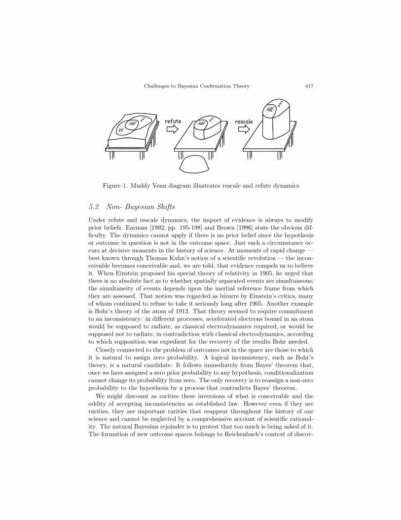
Challenges to Bayesian Confirmation Theory 417
Figure 1. Muddy Venn diagram illustrates rescale and refute dynamics
5.2 Non- Bayesian Shifts
Under refute and rescale dynamics, the import of evidence is always to modifyprior beliefs. Earman [1992, pp. 195-198] and Brown [1996] state the obvious dif-ficulty. The dynamics cannot apply if there is no prior belief since the hypothesisor outcome in question is not in the outcome space. Just such a circumstance oc-curs at decisive moments in the history of science. At moments of rapid change —best known through Thomas Kuhn’s notion of a scientific revolution — the incon-ceivable becomes conceivable and, we are told, that evidence compels us to believeit. When Einstein proposed his special theory of relativity in 1905, he urged thatthere is no absolute fact as to whether spatially separated events are simultaneous;the simultaneity of events depends upon the inertial reference frame from whichthey are assessed. That notion was regarded as bizarre by Einstein’s critics, manyof whom continued to refuse to take it seriously long after 1905. Another exampleis Bohr’s theory of the atom of 1913. That theory seemed to require commitmentto an inconsistency: in different processes, accelerated electrons bound in an atomwould be supposed to radiate, as classical electrodynamics required, or would besupposed not to radiate, in contradiction with classical electrodynamics, accordingto which supposition was expedient for the recovery of the results Bohr needed.
Closely connected to the problem of outcomes not in the space are those to whichit is natural to assign zero probability. A logical inconsistency, such as Bohr’stheory, is a natural candidate. It follows immediately from Bayes’ theorem that,once we have assigned a zero prior probability to any hypothesis, conditionalizationcannot change its probability from zero. The only recovery is to reassign a non-zeroprobability to the hypothesis by a process that contradicts Bayes’ theorem.
We might discount as rarities these inversions of what is conceivable and theoddity of accepting inconsistencies as established law. However even if they arerarities, they are important rarities that reappear throughout the history of ourscience and cannot be neglected by a comprehensive account of scientific rational-ity. The natural Bayesian rejoinder is to protest that too much is being asked of it.The formation of new outcome spaces belongs to Reichenbach’s context of discov-

418 John D. Norton
ery. Bayesian confirmation theory, indeed any logic at all, cannot be responsibleboth for logical relations among propositions and also for the discovery methodsused to create new outcome spaces.
5.3 Is Bayes’ Theorem Sensitive Enough to the Connections betweenEvidence and Theory?
The simplicity of refute and rescale dynamics invites the next challenge: the dy-namics is too simple and too insensitive to the ways that evidence and theory canrelate.
5.3.1 Problems Arising from “Refute. . . .”
The first “refute” step of Bayesian conditionalization depends essentially on theidea that the disjunctive part of H = (H&E) ∨ (H& ∼E) that extends beyondthe total evidence E, that is H& ∼E, does not affect the bearing of evidence Eon H. That is, “narrowness” directly asserts that P (H|E) = P (H&E|E). Whilethis idea is so familiar as generally to pass without comment, it does represent ablindness in Bayesian confirmation theory. As an illustration of it, imagine that weseek to identify some animal. Our evidence is that it is a bird. What support doesthat evidence lend to the possibility that the animal is a canary or, alternatively,a canary or a whale? Narrowness asserts that it lends the same support:
P (canary or whale | bird) = P (canary | bird)
In some scenarios, this can make sense. As we check instances of birds, we willfind the frequency of “canary or whale” to arise exactly as often as “canary.” Ifthese frequencies are all that matters, then we would say the two outcomes areequally supported. However few would halt there. We would discount the “whale”disjunct as a nuisance embellishment that should be dismissed as a distractionprecisely because it is deductively refuted by the evidence “bird.” The frequencycount just mentioned is blind to its nuisance character in so far as it assigns thesame frequency of success to “canary” as to “canary or whale.”
It is possible to devise a logic that is sensitive to this problem and punishes anhypothesis in the degree that it extends beyond the evidence. An example37 is the“specific conditioning” logic defined in [Norton, forthcoming b, Section 10.2]. In aformulation compatible with developments here, the logic amounts to a new defi-nition for the conditional probability P (H|E). It starts with an additive measure
37Specific conditioning resembles some of the measures of incremental support that have beeninvestigated in the Bayesian literature, such as the ratio measure r(H, E) = P (H|E)/P (H) =P (H&E)/(P (E).P (H)). (See [Eels and Fitelson, 2002].) The two differ essentially. The incre-mental measures are functions of three arguments, H, E and B, that represent the incrementalsupport accorded H by evidence E alone with respect to a tacit background B. PSC(H|E) isa function of two arguments, H and E&B, that measures the total support accorded to H byevidence E conjoined with the background B, that is, by the total evidence E&B.
Challenges to Bayesian Confirmation Theory 419
P (.) on the background and defines the alternative
PSC(H|E) = P (H&E)2/(P (E).P (H)) = P (H&E)/(P (E).P (H&E)/(P (H)(SC)
This alternative rule of conditionalization rewards hypotheses H with more supportthe closer they come to the total evidence E = (E and background) — hence theterm “specific conditioning.” PSC(H|E) = 1 only when H = E excepting measurezero differences. H can differ from E in two ways and the logic of (SC) penalizes itfor both. In the first way, H can fail to exhaust E in measure. Then the first factorof (SC), that is, P (H&E)/(P (E), is less than one (which alone would correspondto the usual case of Bayesian conditionalization). In the second way, H can extendbeyond E in measure. Then the second factor of (SC), that is P (H&E)/(P (H), isless than one. Deviations in both ways are penalized equally and it turns out thatthis is expressed in a striking symmetry in PSC . That is PSC(H|E) = PSC(E|H).
Returning to the bird example, with plausible values for PSC(.), we will have
PSC(canary or whale | bird) < PSC(canary | bird)
Indeed we will have
PSC(canary or whale | canary) < PSC(canary | canary) = 1
That is, even though “canary” deductively entails “canary or whale,” the latteris not accorded full support from “canary.” The logic of (SC) judges “canary orwhale” to be supported less specifically by the evidence “canary.” In the case ofBayesian confirmation theory, evidence accords unit support to any of its deductiveconsequences, no matter how much they are weakened logically. PSC reduces thesupport accorded to these deductive consequences according to how much they areweakened logically.
5.3.2 Problems Arising from “. . .Rescale”
In the special case in which they hypothesis H deductively entails the evidenceE, the first “refute” step of Bayesian conditionalization is not invoked and theprocess reduces to rescaling only by means of the property “multiplication” (M).This special case provides a means of isolating the second step and plumbing itsproblems.
Consider two hypotheses H and H ′ both of which entail the evidence E. In thatcase, it follows from Bayes’ theorem that the ratio of the posterior probabilitiesP (H|E)/P (H ′|E) is the same as the ratio of the priors. It now follows thatthe incremental confirmation, as measured by the ratio of posterior and priorP (H|E)/P (H), is the same in both cases. That is, when two hypotheses bothentail the same true evidence, they get the same confirmatory boost. In particular,if H is more probable than, less probable than or just as probable as H ′ prior toconditionalization, it will remain so afterwards.
420 John D. Norton
This failure to separate H and H ′ evidentially, according to critics, is to overlookthat their entailments of the evidence E can differ in more subtle qualities thathave epistemic import. For example, recall efforts in the late 19th century to detectthe earth’s motion through the luminiferous ether. These experiments yielded anull result (E). We may entertain two hypotheses:
H: There is no ether state of rest against which the earth can move.
H ′: There is an ether state of rest but we happen to be motionlesswith respect to it each time the experiments are performed.
Each of H and H ′ entail the evidence E, but it seems wrong that both shouldreceive the same support from E. H succeeds, as it were, by honest toil; butH ′ by theft. There are many ways that this metaphor of honest toil and theft isexplicated.
One way notes that H succeeds because it explains why the experiments yieldednull results, where as H’ does not. Considerations like this lead Achinstein [2001,Ch. 7] to argue that it is not sufficient to count as evidence that some datumincrementally increases the probability of an hypothesis or that the probability ofthe hypothesis conditioned on the datum is high.38 In addition there must be anexplanatory connection.
Other approaches are variants of this idea that some successful entailmentsare virtuous and others not. The hypothesis H makes the prediction that allether current experiments will fail and that prediction is verified by the evidence.Since H ′ supposes that it is by happenstance that we were at rest in the etherjust at the moment of the experiments, H ′ simply accommodates the evidencein the sense that it has been adjusted to accommodate experimental reports athand. Predictions, for example, are virtuous and their success merits an increase inbelief; accommodations are not virtuous and are epistemically inert. See [Horwich,1982, Ch. 5] for discussion and an argument that we should not differentiallyreward prediction and accommodation. Another way of expressing these concernsis to note that H ′ (but not H) was cooked up “ad hoc” specifically to matchthe evidence. A classic example is the creationist hypothesis that the world wascreated in 4004 BC, complete with a fossil record that perfectly simulates a moreancient, evolutionary past. It is an evidential truism that such ad hoc hypothesesgain no support from the observations they accommodate. For an account of howad hoc hypotheses can be treated in a Bayesian context, see [Howson and Urbach,2006, pp. 121-126], who also suggest that sometimes there are “good” ad hochypotheses that deserve support.
The literature on these evidential virtues in Bayesian confirmation theory islarge and convoluted. In general, however, there are two broad strategies thatBayesian confirmation theory can employ when faced with a virtuous and non-virtuous pair of hypotheses. The first is to expand the outcome space so that there
38See [Achinstein, 2001, Ch.7]and passim) for numerous examples. For example, learning thatmost lottery tickets were unsold may increase greatly my belief that mine is the winning ticket,even though the absolute probability may remain small. See also [Laudan, 1997].

Challenges to Bayesian Confirmation Theory 421
are more resources available to pick the hypotheses apart.39 That risks merelypostponing the problem since it may now return for another pair of hypothesesin the larger space. The second is to use prior probabilities to reward virtuoushypotheses and punish non-virtuous ones. That is, since the ratio of the posteriorprobabilities P (H|E)/P (H ′|E) equals the ratio of the priors P (H)/P (H ′), wemay reward the explanatory, predictive or non-ad hoc H by making the ratioP (H)/P (H ′) very large, so that there is a corresponding advantage for H in theposterior probabilities. As observed in [Norton, 2007, §5.3.3], this use of priorprobabilities requires a curious prescience: we are to penalize the prior probabilityof an ad hoc hypothesis in advance in just the right degree so that the punishmentperfectly cancels the as yet unknown confirmatory reward that will be accorded tothe hypotheses by Bayes’ theorem. Further, prior probabilities for hypotheses ortheories are assigned once, globally, whereas virtues are manifested locally and maydiffer from domain to domain. So we may find a theory explanatory in one domainand want to reward it with a high prior probability; but may find it explanatorilydeficient in another, and may want to punish it with a low prior probability.
5.4 The “Likelihood Theory of Evidence” and “Likelihoodism”
The above discussion has dealt with the case of hypotheses that entail the evi-dence. Matters are slightly more complicated when the hypothesis only makes theevidence more or less probable. In that case, Bayes’ theorem allows us to comparethe import of evidence E for two hypotheses H and H ′ as
P (H|E)
P (H ′|E)=
P (E|H)
P (E|H ′)
P (H)
P (H ′)(B′)
It follows that the relative import of the evidence E is fully determined by thetwo likelihoods, P (E|H) and P (E|H ′). For the ratio of the prior probabilitiesP (H)/P (H ′) reflects our comparative belief in H and H ′ prior to any considerationof evidence E; the ratio of the posteriors P (H|E)/P (H|E′) reflects our comparativebelief in H and H ′ after the import of evidence E has been accommodated. Theratio of the likelihoods P (E|H)/P (E|H ′) is what takes us from the ratio of theprior to the ratio of the posteriors. Therefore, it expresses the relative import ofevidence E on these two hypotheses.
That the likelihoods capture all needed information for evaluating the bearingof evidence is the core notion of a “likelihood theory of evidence.” (In the specialcase in which the hypotheses entail the evidence, P (E|H) = P (E|H ′) = 1. Thenthe ratio of the posteriors equals the ratio of the priors and E cannot discriminateevidentially between H and H ′.)
Since so many of the problems of Bayesian confirmation theory focus on priorprobabilities, an attractive modification to the theory is a view that excises prior
39For example Maher treats prediction and accommodation by supposing that hypotheses aregenerated by methods that may or may not have certain items of evidence available to themwhen they generate the hypotheses. He then shifts assessment to the credibility of the methods.See [Achinstein, 2001, pp. 215-221] for discussion.
422 John D. Norton
probabilities but leaves the rest intact. The view, popularly known as “likelihood-ism,” has been advocated by Edwards [1972] and Royall [1997]. As we have justseen, in Bayes’ theorem (B′), the evidence E favors the hypothesis H over H ′ justin the ratio of their likelihoods, P (E|H)/P (E|H ′). The proposal is that this con-sequence of Bayes’ theorem be extracted and elevated to an independent principle,the “law of likelihood.” The judgment of evidential import is always comparative— evidence favors this hypothesis more or less than that — and the troublesomeprior probabilities never need enter.
The principal difficulty for likelihoodism is that it faces all the problems of theBayesian refute and rescale dynamics recounted here, but without the resourcesof prior probabilities to ameliorate them. In particular, likelihoodists must saythat evidence entailed by two hypotheses is equally favorable to both hypothesesno matter what their virtues or vices. For likelihoodists have lost the Bayesianmechanism of using prior probabilities to reward simpler hypotheses or ones withanticipated predictive power and to penalize ad hoc or contrived hypotheses. Roy-all [1997, §1.7] considers and offers likelihoodist rejoinders to such concerns.
5.5 Model Selection, Prediction and Simplicity
While the notion that the likelihoods capture the incremental import of evidencehas enjoyed notable successes, its overall history has been troubled. There arerecalcitrant cases in which the likelihoods alone are clearly too coarse a measure ofthe import of evidence. Likelihood rewards only accuracy in fitting data at hand.It has difficulty accommodating our common preference for simpler hypothesesthat may be less accurate. In rewarding fit to the data at hand, likelihood may bea weaker guide to the greater truth sought that extends beyond these data; that is,likelihood tends to favor accommodation to present data as opposed to predictivesuccess with future data.
The familiar and long-standing illustration of these difficulties comes in theproblem of curve fitting. Let us say that we wish to find the relationship betweenvariables x and y:40
〈x1, y1〉 = 〈0.7, 1.0〉, 〈x2, y2〉 = 〈1.5, 1.8〉, 〈x3, y3〉 = 〈2.1, 2.0〉, . . ., (DATA)
which are shown on the graph of Figure 2 below. Our presumption is that thesedata were generated by the relation
yi = f(xi) + errori
where errori is a random error term affecting the i-th pair of x − y values. (Itis common to assume that these error terms are normally distributed and inde-pendent of one another.) The goal of our analysis is identification of the function
40The full data set is 〈0.7, 1.0〉, 〈1.5, 1.8〉, 〈2.1, 2.0〉, 〈2.3, 0.6〉, 〈2.6, 1.0〉, 〈3.8, 2.1〉, 〈4.5, 3.1〉,〈4.7, 6.0〉, 〈5.6, 6.9〉, 〈5.6, 7.7〉, 〈5.8, 4.9〉, 〈6.2, 4.4〉, 〈7.1, 7.7〉, 〈7.6, 6.7〉, 〈8.8, 10.1〉, 〈8.9, 8.2〉,〈9.1, 8.1〉, 〈9.3, 7.4〉.

Challenges to Bayesian Confirmation Theory 423
f(x). The standard method is to find that function that generates a curve of bestfit to the data. For data such as in Figure 2, we would normally seek a straightline. That is, we would assume that the unknown function is linear, so that thedata was generated by
yi = A + Bxi + errori (LIN)
That straight line turns out to be
yi = −0.332 + 0.997xi + errori (LINbest)
The straight line LINbest is the best fit to the data in the sense that it is thestraight line drawn from LIN that makes the DATA most probable. That is, itsvalues of A and B maximize the likelihood P (DATA | LINbest); and A = −0.332and B = 0.997 are the “maximum likelihood estimators” of A and B.
Figure 2. Linear and cubic curves of best fit
The complication is that we can find other functions f(x) that fit the data moreclosely and make it even more probable. Consider, for example, cubic functions
yi = A + Bxi + Cx2i + Dx3
i + errori (CUB)
The particular cubic plotted in Figure 2 against the background of the samedata,
yi = 1.952 − 1.377xi + 0.581x2i − 0.0389x3
i + errori (CUBbest)
maximizes the likelihood P (DATA | CUBbest).As one can see from comparing the two curves visually, the cubic CUBbest fits
the data more closely that the linear LINbest and it turns out that
P (DATA| CUBbest) > P (DATA | LINbest)

424 John D. Norton
Therefore, according to the likelihood theory of evidence, we should concludethat the data better supports the cubic CUBbest over the linear LINbest.
It is evident from a cursory scan of the data that this is most likely a mistake.Whatever trend f(x) may be embodied within the data, it is heavily confoundedby noise from the error term. While the data definitely gives us warrant to believethat f(x) is an increasing function of x, we have no warrant for the specifics of thecubic CUBbest.41 We should be much more modest in what we infer from data thisnoisy. The better fit of the cubic CUBbest has been achieved by the greater abilityof a cubic to conform to random fluctuations from the trend induced by noise;that is, the curve is “overfitted.” This overfitting is most evident around x = 1,where the curve reverses direction; and again around x = 9, where the curve alsoreverses direction. Given the sparsity and scattering of the data, cubic CUBbest ismerely tracking noise at these places, whereas the linear LINbest is responding toa real increase with x in the trend.
The informal discussion of the last paragraph captures the practical thinkingof curve fitting. It is grounded tacitly in the considerations of simplicity andprediction at issue here. We know that we can always find a curve that fits thedata better by looking to more complicated functional forms, such as higher orderpolynomials. However, at some stage, we judge that we should prefer the simplercurve over the more complicated one that fits the data better. The reason is thatour interests extend beyond the narrow problem of finding a curve that merelyfits this particular data set well. Our data is only a sample of many more valuesof x and y; and we are interested in finding a function f(x) that will also fitthese other as yet unseen values. That is, our goal is to find a function f(x)that will support prediction. We expect that we can best achieve that goal byforgoing some accuracy of fit with the present data of an overfitted curve in favorof a simpler functional form for f(x) that will enable future data to be fittedbetter. For an overfitted curve responds to random noise whose specific patternsof deviations will probably not reappear in future data; however a curve drawnfrom the simpler model responds more to the real relation that drives present and,we suppose, future data as well.
The challenge to a Bayesian analysis is to find a way of capturing these lastinformal thoughts in a more precise analysis. The natural way to do this is tobreak up the inference problem into two parts.42 The first part requires us toconsider only models. These are sets of hypotheses indexed by parameters. Forexample, LIN above is the set of linear functions with parameters A and B takingall real values. CUB above is the set of all cubic functions with the parametersA,B,C and D taking all real values. In the first part we decide which model is
41Perhaps it is unfair to introduce a more elevated perspective that affirms this judgmentagainst the cubic CUBbest. The data plotted was generated artificially from the model yi = xi
+ errori, so the linear LINbest has actually done a very good job of identifying the trend y = x.42Traditional non-Bayesian statistical methodology implements this two part procedure by
testing whether deviations in the coefficients B and C of CUB from zero are statistically signif-icant. If they are not, the null hypothesis of B=C=0 is accepted and estimation proceeds withthe simple model LIN.
Challenges to Bayesian Confirmation Theory 425
appropriate to the data. For DATA above, we presume that would turn out to beLIN and not CUB. In the second part of the inference problem, we then find thecurve that fits the data best just within that selected model.
Implementing this program within Bayesianism runs into several difficulties.The functions of LIN are a subset of those of CUB, for CUB reverts to LIN if weset C = D = 0. So if we compute the posterior probabilities of the models on theDATA, we will always find
P(LIN | DATA) ≤ P(CUB | DATA)
from which it follows that that the model LIN can never be more probable on theDATA than the model CUB. So it seems that we cannot have a straightforwardBayesian justification for preferring LIN over CUB.
Slightly less than straightforward grounds can be found. We compare notthe posterior probabilities of models, but the boosts in probability each modelsustains upon conditionalizing on the data. That is, in this modified approach,we would prefer LIN over CUB if the ratio P (LIN | DATA) / P (LIN) exceedsP (CUB | DATA) / P (CUB). The ratio of these two ratios is itself called the“Bayes’ factor.”
This modified criterion of the Bayes’ factor has some plausibility since it con-forms to the spirit of the likelihood theory in that we consider changes in prob-ability under conditionalization, not absolute values of the posterior probability.However the modified criterion rapidly runs into difficulties with prior probabil-ities. To compute P (LIN | DATA), for example, we would use Bayes’ theorem,in which the likelihood P (DATA | LIN) appears. This likelihood is really a com-pound quantity. It is a summation over the infinitely many curves that appear inthe model LIN, corresponding to all possible values of A and B. That is,
P (DATA|LIN) =
∫
allA,Bp(DATA|A,B)p(A,B)dAdB
The problematic term is p(A,B), which is the prior probability density for theparameters A and B given that LIN is the correct model. Since it expresses ourdistribution of belief over different values of A and B prior to evidence, p(A,B)should favor no particular values of A or B. However it is familiar problem thatno probability distribution can do this. If p(A,B) is any non-zero constant, thenit cannot be normalized to unity when we integrate over all possible values of Aand B.
While no unqualified solution to these problems has emerged, it has provenpossible to show that, for large data sets, the Bayes factor depends only weakly onthe choice of the prior probability density. In that case, the model favored by theBayes factor is the one that maximizes what is known as the Bayes InformationCriterion (BIC):
BIC = log Lbest – (k/2) log n

426 John D. Norton
where the maximum likelihood Lbest is the likelihood of the data when condition-alized on the best fitting curve in the model, k is the number of parameters in themodel and n is the size of the data set. (For LIN, k is 2; for CUB, k is 4.) Forfurther discussion, see [Wasserman, 2000].
In maximizing BIC, we tradeoff accuracy of fit (expressed in the maximizingof likelihood) against the simplicity of the model (expressed in the number of pa-rameters k). This was not the goal in constructing BIC; it was generated from ananalysis that seeks the most probable model on the evidence. An analogous crite-rion can be generated by directly seeking the model with the greatest predictivepower, as opposed to the one that is most probable. This criterion, the AkaikeInformation Criterion (AIC), advocated by Forster and Sober [1994], is given by
AIC = log Lbest − k
The rationale is that overtly seeking predictive power is a surer way to get to atruth that extends beyond the particular data at hand. Seeking the most probablemodel risks favoring the vagaries of the particular data at hand.
The connection to prediction is achieved through the notion of “cross-validation.”While we cannot now test the predictive powers of a model against presently un-known data, we can simulate such a test by dividing the data at hand into twoparts. We use the first part to generate a best fitting hypothesis in the model andthen we check how well the resulting hypothesis fits the remaining data. In a largeset of N data, we leave out one datum and use the remaining N − 1 to generatehypotheses from the model. We then average the errors in fitting the originaldatum. If we allow each datum successively to be left out in the procedure andaverage the resulting scores, we recover an estimate of the predictive powers ofthe model. That estimate turns out to approach the AIC statistic for large N .[Forster, 2002, p. S128; Browne, 2000]. The presumption is that predictive powersmanifested within a known data set in this computation will persist beyond theconfines of that data set.
It remains an open question whether likelihoods may be used as the basis ofassessment of models when we need to find an appropriate accommodation ofaccuracy, simplicity and predictive power. That all the proposals above fail hasbeen suggested recently by Forster [2006; 2007]. He has devised examples of pairs ofmodels with the same number of parameters k that also deliver the same likelihoodand maximum likelihood for a specified set of data. As a result, considerationsof likelihood alone or the more refined BIC or AIC are unable to discriminatebetween the models. However it is evident from informal considerations that onemodel is predictively superior to the other.
Forster’s simplest example43 draws on a set of data with three points 〈xi, yi〉:
〈1, 1〉, 〈2, 2〉, 〈3, 3〉 (DATA′)
43This example was presented in a talk by Malcolm Forster, “Is Scientific Reasoning Reallythat Simple?” in “Confirmation, Induction and Science” London School of Economics, March 8– March 10, 2007, on March 8.
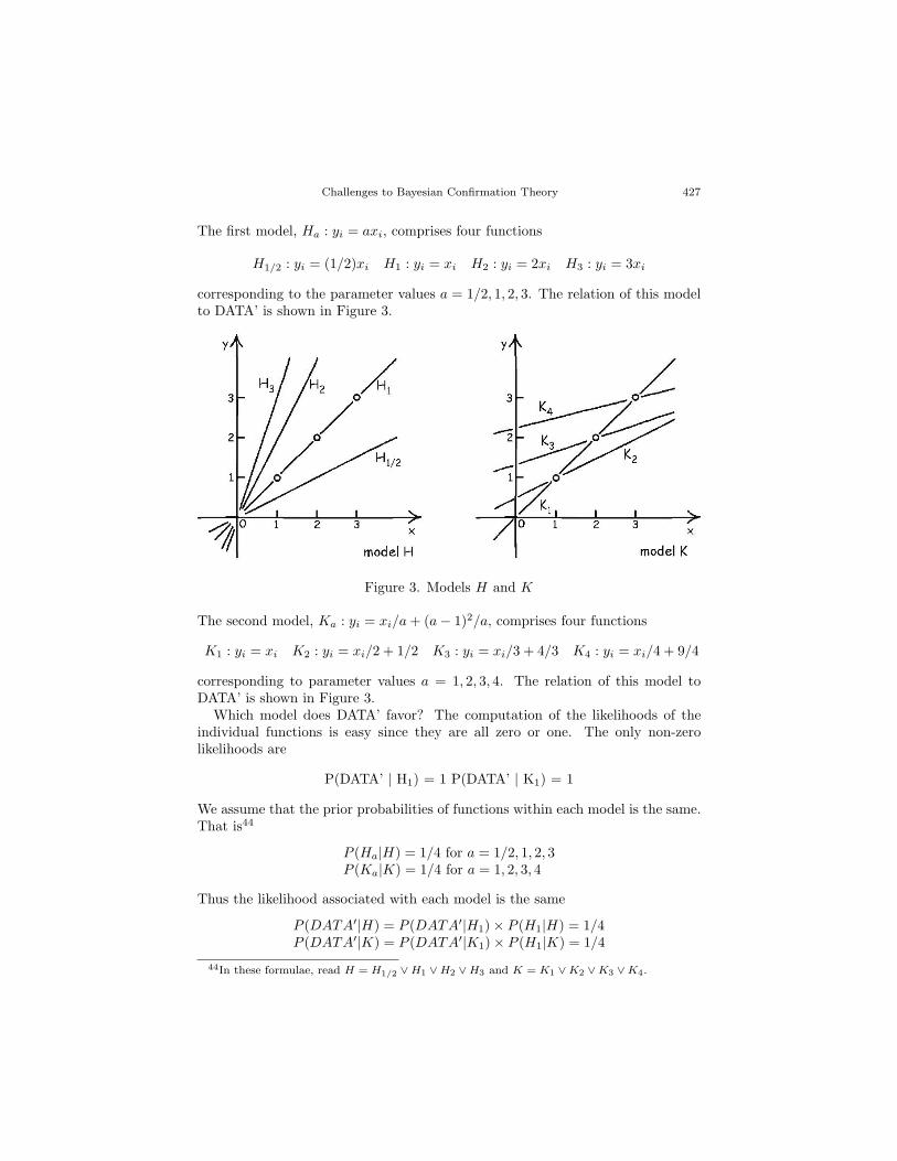
Challenges to Bayesian Confirmation Theory 427
The first model, Ha : yi = axi, comprises four functions
H1/2 : yi = (1/2)xi H1 : yi = xi H2 : yi = 2xi H3 : yi = 3xi
corresponding to the parameter values a = 1/2, 1, 2, 3. The relation of this modelto DATA’ is shown in Figure 3.
Figure 3. Models H and K
The second model, Ka : yi = xi/a + (a − 1)2/a, comprises four functions
K1 : yi = xi K2 : yi = xi/2 + 1/2 K3 : yi = xi/3 + 4/3 K4 : yi = xi/4 + 9/4
corresponding to parameter values a = 1, 2, 3, 4. The relation of this model toDATA’ is shown in Figure 3.
Which model does DATA’ favor? The computation of the likelihoods of theindividual functions is easy since they are all zero or one. The only non-zerolikelihoods are
P(DATA’ | H1) = 1 P(DATA’ | K1) = 1
We assume that the prior probabilities of functions within each model is the same.That is44
P (Ha|H) = 1/4 for a = 1/2, 1, 2, 3P (Ka|K) = 1/4 for a = 1, 2, 3, 4
Thus the likelihood associated with each model is the same
P (DATA′|H) = P (DATA′|H1) × P (H1|H) = 1/4P (DATA′|K) = P (DATA′|K1) × P (H1|K) = 1/4
44In these formulae, read H = H1/2 ∨ H1 ∨ H2 ∨ H3 and K = K1 ∨ K2 ∨ K3 ∨ K4.

428 John D. Norton
Hence, we cannot use DATA’ to discriminate between the two models H and K bymeans of their maximum likelihoods or the likelihoods of the models. Moreover,we cannot discriminate between them by means of BIC or AIC; for both modelsagree on the maximum likelihood and the number of parameters, k = 1.
While all the likelihood based instruments fail to discriminate between the mod-els, informal considerations favor the model H. For it requires only one datumfrom DATA’, such as 〈1, 1〉, to fix the function y = x in H that fits the remainingdata. The remaining two data points act as tests of the model; or, we may viewthem as successful predictions. However it takes two data points from DATA’ tofix the function in K that fits the remaining data. The datum 〈1, 1〉, for example,is compatible with both K1 and K2. A second datum is needed to decide betweenthem. Hence only one datum remains to test the function fitted; or the modelneeds more data before it can make successful predictions. As a result we infor-mally judge that the model H is better tested and predictively stronger and thusbetter warranted by the evidence. (For discussion of this aspect of curve fitting,see [Glymour, 1980, Ch. VIII.])45
For further discussion of Bayesian and Likelihood based analyses of this prob-lem, see [Howson and Urbach, 2006, 288-96] and [Forster and Sober, 2004] (whichincludes commentary by Michael Kruse and Robert J. Boik).
5.6 A Neutral Starting Point: The Second Problem of the Priors
Bayesian confirmation theory depicts learning from evidence as the successive con-ditionalization of a prior probability distribution on evidence so that the resultingposterior probability distributions increasingly reflect just the evidence learned.As we trace back along this chain of conditionalization, we expect to come to epis-temically more neutral probability distributions, reflecting our lesser knowledgeearlier in the process. The problem of the priors in both forms developed here isthat the structure of Bayeisan confirmation theory essentially precludes neutralprobability distributions. In the first problem of the priors (Section 4.3 above), wesaw that the additivity of probability measures precludes their representing epis-temic states of complete ignorance. Here we shall see that the Bayesian dynamicsof refute and rescale also precludes a different sort of neutrality of the probabilitydistribution. Bayesian dynamics makes it impossible to select a prior probabilitydistribution that does not exercise a controlling influence on subsequent course ofconditionalization.46
The essential problem is suggested by the notion of refute and rescale dynamics.The results of conditionalization must already be present in the prior probability;all that conditionalization does is to remove those parts of the prior probability
45The informal considerations invoked here may appear more familiar if we vary the exampleslightly. Imagine that we are to choose between the model H : y = ax and L : y = ax + b forDATA′. Then we would allow that H is better warranted since a single datum is needed to fixthe parameter a in H; whereas two data are needed to fix the two parameters a and b in L.
46The phrase “problem of the priors” seems to mean somewhat different to things to differentauthors. For further discussion, see [Earman, 1992, pp. 57-59; Mellor, 2005, pp. 94-95].

Challenges to Bayesian Confirmation Theory 429
distribution attached to outcomes refuted by the evidence to reveal the pre-existingdistribution of belief between the unrefuted outcomes. This same point is evidentif we recall the formula governing conditional probabilities
P (H|E) = P (H&E)/P (H)
This formula tells us that P (H|E), the degree of belief we should have in Hgiven that we have learned E, is fixed by the two prior probabilities P (H&E)and P (H). That means that if we fully specify our prior probabilities over someoutcome space, we have also delivered an exhaustive catalog of what our beliefin each outcome would be, given that we have learned some other outcome. Forfrom being neutral, the prior probability distribution anticipates how our beliefswill evolve as we learn any sequence of admissible outcomes and different priorprobability distributions can yield courses that differ greatly. This considerationgives further grounds for the abandoning of such terms as “ignorance priors” or“informationless priors” in favor of “priors constructed by some formal rule” asreported in Section 4.4 above.
As with the first problem, objectivists have the most acute difficulty with thissecond problem of the priors. For they are committed to there being one, appro-priate prior probability distribution in any given epistemic situation. Yet none cansupply the neutral starting point appropriate in the absence of all evidence. Sothe objectivist must either accept the unpalatable conclusion that the initial priorprobability contains information without evidential warrant; or that Bayesian dy-namics can only be used once we have learned enough by other means to make aproperly grounded selection of the prior probability.
Subjectivists at first seem to have a better response. For them, a prior proba-bility is simply a statement of personal opinion with no pretensions of evidentialwarrant. As evidence accumulates and is incorporated into the probability dis-tributions by conditionalization, limit theorems assure us of a merging of opiniononto a unique distribution that properly represents the bearing of evidence. (Fordiscussion of these theorems, see [Earman, 1992, Ch. 6].) However this solutioncomes at some cost. At any finite stage of the process, the posterior probabilitydistribution is an unknown mix of unwarranted opinion and warranted support.While the limit theorems may assure us that, in particular circumstances, the mixwill eventually converge onto warranted support, at any definite state we may bearbitrarily far from it.47 Imagine that we have collected some very large set ofevidence Elarge and we are interested in its bearing on some hypothesis H. It willalways be possible for a determined mischief maker to identify some prior prob-abilities for P (H&Elarge) and P (Elarge) so that P (H|Elarge) is as close to oneas you like or as close to zero as you like. The two differ essentially. The incre-mental measures are functions of three arguments, H,E and B, that represent theincremental support accorded H by evidence E alone with respect to a tacit back-ground B. PSC(H|E) is a function of two arguments, H and E&B, that measures
47Here is the obligatory reporting of Keynes’ quip: “In the long run we are all dead.”

430 John D. Norton
the total support accorded to H by evidence E conjoined with the background B,that is, by the total evidence E&B.
5.7 The Prior Probability of Universal Generalizations
Neither objectivist nor subjectivist fares well if zero or unit prior probability hasbeen assigned injudiciously to some outcome. Then Bayesian dynamics becomescompletely dogmatic. For once they have been assigned zero or unit probability, itfollows from Bayes’ theorem that these assignments are unrevisable by condition-alization.48 The complete disbelief of a zero prior probability and the completebelief of a unit probability will persist indefinitely. In concrete terms, this sort ofdogmatism is a familiar if unwelcome phenomenon. Consider the dogmatic con-spiracy theorist who discounts the benign explanation of a catastrophe in favor ofan elaborate conspiracy committed by some secret agency. Once a zero prior prob-ability has been assigned to the benign explanation, no failure to reveal the secretagency’s intervention or even existence can restore belief in the benign explana-tion. Rather Bayes’ theorem will provide mounting assurance that each failure isfurther evidence of the perfection of the secret agency’s cover-up.
While the best Bayesian advice would seem to be very cautious before assigninga zero prior probability, there are suggestions, reviewed in more detail in [Earman,1992, §4.2, 4.3], that hypotheses with the power of universal generalizations oughtto be assigned a zero prior probability. These concerns arise for any hypothesesH that entails a countable infinity of consequences E1, E2, . . . 49 Considering onlythe first n consequences we have
P (H) = P (H|E1&. . .&En).P (En|E1&. . .&En−1).P (En−1|E1&. . .&En−2).. . .P (E2|E1).P (E1)
Popper [1959, Appendix VII] urged that we should expect the instances E1, E2,. . . of a universal generalization H to be equiprobable and independent of oneanother. That is,
P (En|E1&. . .&En−1).P (En−1|E1&. . .&En−2).. . .P (E2|E1).P (E1)= P (En).P (En−1).. . .P (E2).P (E1) = P (E1)n
But since this must hold for arbitrarily large n and with P (E1) < 1, it follows thatthe prior P (H) = 0. The obvious weakness of Popper’s proposal is that the veryfact that E1, E2, . . . are instances of a universal generalization H suggests thatthey are not independent. However, just a little dependence between E1, E2, . . .is not enough to allow a non-zero prior for H. Inspection of the above expressionfor P(H) shows that P (H) > 0 entails
48Once P (H) = 0, Bayes’ theorem (B) requires P (H|E) = 0 for all admissible E. (Condition-alizing on evidence E for which P (E) = 0 leads to an undefined posterior P (H|E).) It followsthat for any H′ =∼H for which P (H′) = 1, P (H′|E) = 1 as well.
49The simplest example is a universal generalization that asserts, “For all x, Q(x).” where xranges over a countably infinite set of individuals a, b, c, . . . Its consequences are Q(a), Q(b), . . .
Challenges to Bayesian Confirmation Theory 431
Limn→∞P (En|E1&. . .&En−1) = 1
That is, finitely many favorable instances of H eventually make us arbitrarily surethat the next instance will be favorable. That was an outcome that Jeffrey [1983,p. 194] felt sufficiently akin to “jumping to conclusions” to want to renouncenon-zero prior probabilities on universal hypotheses.
Lest this commitment to the projectability of the hypothesis not seem immodest,the analysis needs only a slight modification to make it more striking. Group theinstances E1, E2, . . . into sets that grow very rapidly in size. For example
F1 = E1 F2 = E2&. . .&E10 F3 = E11&. . .&E100. . .
so that
F1&. . .&Fn = E1&. . .&E(10n−1)
Each of the Fi is a consequence of H, so the above analysis can be repeated withFi substituted for Ei to infer that p(H) > 0 entails
Limn→∞P (E1&. . .&E(10n+1)|E1&. . .&E(10n)) = 1
That is, if we assign non-zero prior probability to an hypotheses with the powerof a universal generalization, eventually we are willing to project from some finiteset of its positive instances to arbitrarily many more at arbitrarily high probability.
The point is not that there is something intrinsically wrong with such immod-esty. Indeed for the right hypothesis, this may be just the appropriate epistemicattitude. The point is that assigning a zero or a non-zero prior probability toa hypothesis with the power of a universal generalization is never neutral. Theformer commits us dogmatically never to learning the hypothesis; the second, nomatter how small the non-zero prior, commits us to its arbitrary projectability onfinite favorable evidence. There is no intermediate value to assign that leaves ouroptions open. Our inductive course is set once the prior is assigned.
Finally, one sees that some significant prior knowledge is needed if we are toassign the non-zero prior probabilities prudently. For a countably infinite set ofoutcomes E1, E2, . . . corresponds to an uncountable infinity of universal hypothe-ses: each hypothesis corresponds to one of the uncountably many combinations ofthe Ei and their negations ∼Ei. However we can assign non-zero prior probabilityto at most countably many of these hypotheses. That is, loosely speaking, whenwe assign our priors, we are selecting in advance the measure zero subset thatwe will be prepared to learn and dogmatically banishing the rest to disbelief nomatter what evidence may accrue.
5.8 Uncertain Evidence
The versions of Bayesian confirmation theory considered so far depict learning asan absolute: if we are given evidence E, it cannot be doubted. That is quite unre-alistic. No datum is ever certain and it is not uncommon in science that the accu-mulation of later evidence leads one to doubt the correctness of evidence collected

432 John D. Norton
earlier. Something like this could be incorporated into traditional Bayesianism ifwe separate, say, the inerrant sense datum D: “my retina senses a plesiosaur likeshape on the surface of Loch Ness” from the fallible evidence E: “I saw a ple-siosaur on Loch Ness.” That fallibility could then enter the analysis through theconditional probability P (E|D). This solution complicates the analysis withoutultimately allowing that all evidence is fallible, for it merely pushes the inerrancydeeper into an elaborated outcome space.
A direct solution has been proposed by Jeffrey [1983, Ch. 11]. StandardBayesianism introduced evidence E by by conditionalizing, which forces unit prob-ability onto E. Jeffrey instead proposed that we merely shift a lesser amount ofprobability to E, commensurate with our confidence in it. This non-Bayesian shiftfrom initial probability Pi to final probability Pf is then propagated through theoutcome space by Jeffrey’s rule. For this simplest case of evidence that partitionsthe outcome space into {E,∼E}, the rule asserts that, for each proposition A,
Pf (H) = Pi(H|E).Pf (E) + Pi(H| ∼E).Pf (∼E)
The distinctive property of this rule is that it leaves unaffected our judgmentswhat the probability of H would be were E definitely true or definitely false. Thatis, for all H, it satisfies Pi(H|E) = Pf (H|E) and Pi(H| ∼ E) = Pf (H| ∼ E).The uniqueness of Jeffrey’s rule follows in that it proves to be the only rule thatsatisfies these two conditions [Jeffrey, 1983, p. 169; Howson and Urbach, 2006,p. 85]. Jeffrey’s rule reduces to ordinary conditionalization if the evidence E iscertain, Pf (E) = 1.
One unappealing aspect of Jeffrey’s rule is that the order in which it is applied insuccessive applications matters. That is, if we apply it first on a partition {E,∼E}and then {F,∼ F}, in general we do not arrive at the same final probabilitydistribution as when the order is reversed. (See [Diaconis and Zabell, 1982].)
In the context of the Shafer-Dempster theory (Section 4.2 above), Dempster’srule of combination allows uncertain evidence to be combined with other beliefdistributions in an analogous way, but one that is independent of the order ofcombining. With appropriate restrictions, Dempster’s rule of combination canyield ordinary Bayesian conditionalization as a special case. See [Diaconis andZabell, 1986] for discussion of the relationship between Jeffrey’s rule and Demp-ster’s rules.
6 FURTHER CHALLENGES
This concluding section collects mention of some of the many further challengesto Bayesian confirmation theory that can be found in the literature.
In a letter to Nature and a subsequent article, Popper and Miller [1983, 1987]urged that the probabilistic support evidence E provides an hypothesis H inBayesian confirmation theory is not inductive support. Their argument dependedupon decomposing H into conjunctive parts by the logical identity

Challenges to Bayesian Confirmation Theory 433
H = (H ← E)&(H ∨ E)
where the first conjunct, “H, if E,” is (H ← E) = (H∨ ∼E). Since the secondconjunct (H ∨ E) is deductively entailed by E, they identify the first, (H ← E),as “containing all of [H] that goes beyond [E]” [1983, p. 687] and require thatE supplies inductive support for H only in so far as it supports this part that isnot deductively entailed by E. However it is easy to show that P (H ← E|E) ≤P (H ← E) so that (H ← E) never accrues probabilistic support from E.
While Popper and Miller’s argument drew much discussion (for a survey see[Earman, 1992, pp. 95-98]), the decisive flaw was already identified immediatelyby Jeffrey [1984], who objected that (H ← E) is not the part of H that goes beyondE. It rests on a confusion of “part” with “deductive consequence.” While we mightthink of theorems as logical parts of the axioms that entail them, that sense ofpart no longer works when inductive relations are the concern. For example, letH be that my lost keys are in my office (“office”) or in my bedroom (“bedroom”)and E is the evidence that they are in my house. Then (H ← E) is the enormousdisjunction
office ∨ bedroom ∨ Mars ∨ Jupiter ∨ Saturn ∨ . . .
where the ellipses include all places not in my house. It is as peculiar to call thisdisjunction a part of the original hypothesis as it is unsurprising that it is notprobabilistically confirmed by the evidence.
Another challenge to Bayesian confirmation theory comes from what first ap-pears as an unlikely source. Over recent decades, there has been a mounting bodyof evidence that people do not assess uncertainty in accord with the strictures ofprobability theory. The most famous example comes from Kahneman and Tver-sky’s [1982] experiments that showed that people are quite ready to contradict themonotonicity of a probability measure — the property that an outcome is neverless probable that each of its logical consequences. In the case of “Linda,” theyfound that people would affirm that a suitably described character Linda is morelikely to be a bank teller and feminist than a consequence of this possibility, thatshe is a bank teller. One response to this body of work is to lament the unreli-ability of people’s intuitions about uncertainty and the need for them to receivetraining in the probability calculus. Another response notes that we humans havebeen dealing more of less successfully with uncertainty for a long time; this successextends to much of science, where uncertainties are rarely treated by systematicBayesian methods. So perhaps we should seek another approach based a littlemore closely on what people naturally do. Cases like “Linda” suggest that we nat-urally try to select the one conclusion that best balances the risk of error againstinformativeness and detach it from the evidence. That is quite compatible withpreferring to detach less probable outcomes. When told a coin was tossed, mostpeople would infer to the outcome “heads or tails” as opposed to “heads or tailsor on edge” even though the latter is more probable and a certainty.

434 John D. Norton
In philosophy of science, if a numerical calculus is used to assess the bearing ofevidence, it is most often the probability calculus. In other domains, that is less so.In the artificial intelligence literature, alternative calculi proliferate. They includethe Shafer-Dempster theory, possibility theory [Zadeh, 1978] as well as numericalsystems generated for particular contexts, such as the MYCIN system applied inmedical diagnostics [Shortliffe and Buchanan, 1985]. One motivating factor hasbeen pragmatic. A probabilistic analysis requires a prohibitively large number ofquantities to be fixed for the general case. In an outcome space with n atomicpropositions, there are of the order of n! conditional probabilities. Seen fromthat perspective, possibility theory’s simple rule for disjunction is appealing: thepossibility of AvB is just the larger of the possibilities of A or B individually. Thatsame rule would seem disastrous to the systematic philosopher of science schooledwith Bayesian intuitions, who will wonder why the rule does not distinguish thecases of A and B coincident or mutually exclusive and all those in between. Thedebate between proponents of the different calculi, including probabilistic systems,has been fierce. The principle goal seems to be to establish that each proponent’ssystem has the same or greater expressive power than another’s. (See for example[Cheeseman, 1986; Zadeh, 1986].)
The issue of “stopping rules” has entered the philosophy of science literaturefrom the debate between Bayesian and Neyman-Pearson statisticians. It pertainsto a deceptively simple plan for assuring belief in a false hypothesis. Assumewe have a fair coin. On average, on repeated tosses, it will show heads with afrequency of about 0.5. The actual frequency will fluctuate from this expected0.5 and there will always be some definite but small probability that the observedfrequency is arbitrarily far removed from the expected. In order to advance themisperception that the coin is not fair, we toss it repeatedly, waiting mischievouslyfor chance to realize one of these rare removals that is possible but very unlikelyfor a fair coin. That is our “stopping rule.” When the rare removal happens wereport the resulting count of heads and tails as evidence that the coin is not fair.The plan can be generalized to seek disconfirmation of any statistical hypothesis.We accumulate observations, waiting for chance fluctuations to deliver results thatcan only arise with low probability if the hypothesis is true.
The result is troubling for Bayesians. For them, the import of evidence is fullydetermined by the likelihood ratio and that likelihood ratio has been contrivedto favor arbitrarily strongly the falsity of the hypothesis. That the experimenterintended to generate a deceptive result is irrelevant; the intentions of the exper-imenter collecting the data do not appear in Bayes’ theorem. Neyman-Pearsonstatisticians have a ready escape that is not available to the Bayeisan: the strat-egy of “try and try again until you get a statistically significant result” is not agood test of the hypothesis. Correspondingly, the procedure that uses this stop-ping rule does not count as a severe test of the hypothesis in the sense of Mayo[1996, §11.3, 11.4].
The Bayesian response has been to reaffirm that the likelihoods are all thatis relevant to discerning the bearing of evidence and also to point out that the
Challenges to Bayesian Confirmation Theory 435
stopping rule may never be satisfied, so that the planned disconfirmation canfail. That is, assume that a Bayesian agent assigns a prior probability p to somehypothesis and decides to accumulate evidence concerning the hypothesis until theposterior probability has risen to q > p. Kadane, Schervisch and Seidenfeld [1996]show that, if the hypothesis is false, the agent’s probability that the stopping ruleis eventually satisfied is given by
Probability of stopping ≤ p(1−q)q(1−p)
Therefore, the closer the desired posterior probability q is set to one, the closerthe probability of stopping comes to zero; that is, the probability as assessed bythe agent approaches one that the experiment will continue indefinitely withoutreturning the result sought in the stopping rule.50 For more discussion see see[Savage et al., 1962, pp. 17-20 and subsequence discussion; Mayo, 1996, §11.3,11.4; and Kadane et al., 1996].
7 CONCLUSION
This chapter has reviewed many challenges to Bayesian confirmation theory. Someare global, reflecting differences in the very conception of inductive inference andthe inductive enterprise in science. Others are more narrowly targeted to specificcommitments of Bayesian confirmation theory. That there are so many challengesis a reflection of the dominance that Bayesian confirmation theory now enjoys inphilosophy of science. It offers a well-articulated account of inductive inference inscience that is of unrivalled precision, scope and power. In this regard it greatlyoutshines its competitors. Abductive accounts — inference to the best explana-tion — are still stalled by the demand for a precise account of their central notion,explanation, whereas Bayesian confirmation theory suffers from the reverse: ex-cessive elucidation of its central notion, probability. This precision and depth ofarticulation is part of what enables the challenges to Bayesian confirmation the-ory to be mounted. For it is only after a position is clearly articulated that itsweaknesses may also be discerned. When a new Goliath enters the arena, manywould be Davids come with their pebbles.
ACKNOWLEDGEMENTS
I am grateful to Malcolm Forster for helpful discussion on an earlier draft.
50If a tenfold boost in probability is sought, so q/p = 10, we must have p ≤ 0.1 to start withand the formula assures us that the probability of stopping is less than (p/q − p)/(1 − p) =(0.1 − p)/(1 − p) < 0.1.
436 John D. Norton
BIBLIOGRAPHY
[Achinstein, 2001] P. Achinstein. The Book of Evidence. New York: Oxford University Press,2001.
[Aczel, 1966] J. Aczel. Lectures on Functional Equations and their Applications. New York:Academic Press, 1966.
[Artzenius, manuscript] F. Arntzenius. Goodman’s and Dorr’s Riddles of Induction.[Bacchus et al., 1990] F. Bacchus, H. E. Kyburg, Jr., and M. Thalos. Against Conditionaliza-
tion, Synthese, 85, pp. 475-506, 1990.[Bartha, 2004] P. Bartha. Countable Additivity and the de Finetti Lottery, British Journal for
the Philosophy of Science, 55, pp. 301-321, 2004.[Bartha and Johns, 2001] P. Bartha and R. Johns. Probability and Symmetry, Philosophy of
Science, 68 (Proceedings), pp. S109-S122, 2001.[Blake et al., 1960] R. M. Blake, C. J. Ducasse, and E. H. Madden. Theories of Scientific
Method: The Renaissance Through the Nineteenth Century. E. H. Madden, ed. Seattle: Uni-versity of Washington Press, 1960.
[Brown, 1994] H. Brown. Reason, Judgment and Bayes’s Law, Philosophy of Science, 61, pp.351-69, 1994.
[Browne, 2000] M. W. Browne. Cross-Validation Methods, Journal of Mathematical Psychology44, pp. 108-132, 2000.
[Carnap, 1950] R. Carnap. Logical Foundations of Probability. Chicago: University of ChicagoPress, 1950.
[Cheesman, 1986] P. Cheeseman. Probabilistic versus Fuzzy Reasoning, pp. 85-102 in L. N.Kanal and J. F. Lemmer, eds., Uncertainty in Artificial Intelligence: Machine Intelligenceand Pattern Recognition. Volume 4. Amsterdam: North Holland, 1986.
[Cox, 1961] R. T. Cox. The Algebra of Probable Inference, Baltimore: Johns Hopkins Press,1961.
[Diaconis and Zabell, 1982] P. Diaconis and S. Zabell. Updating Subjective Probability Journalof the American Statistical Association. 77, pp. 822-30, 1982.
[Diaconis and Zabell, 1986] P. Diaconis and S. Zabell. Some Alternatives to Bayes’s Rule, pp.25-38 in Information and Group Decision Making: Proceedings of the Second Universityof California, Irvine, Conference on Political Economy. B. Grofman and G. Owen, eds.Greenwich, Conn,: JAI Press, 1986.
[Duhem, 1969] P. Duhem. To save the phenomena, an essay on the idea of physical theory fromPlato to Galileo. Chicago, University of Chicago Press, 1969.
[Earman, 1992] J. Earman. Bayes or Bust. Cambridge, MA: Bradford-MIT, 1992.[Earman and Salmon, 1992] J. Earman and W. Salmon. The Confirmation of Scientific Hy-
potheses, ch. 2 in Introduction to the Philosophy of Science. M. H. Salmon, et al. Prentice-Hall, 1992; repr. Indianapoli: Hackett, 1999.
[Eells and Fitelson, 2002] E. Eells and B. Fitelson. Symmetries and Asymmetries in EvidentialSupport, Philosophical Studies, 107, pp. 129-142, 2002.
[Edwards, 1972] A. W. F. Edwards. Likelihood. London: Cambridge University Press, 1972.[Ellsberg, 1961] D. Ellsberg. Risk, Ambiguity, and the Savage Axioms, Quarterly Journal of
Economics, 75, pp. 643-69, 1961.[Feinstein, 1977] A. R. Feinstein. Clinical Biostatistics XXXIX. The Haze of Bayes, the Aerial
Palaces of Decision Analysis, and the Computerized Ouija Board, Clinical Pharmacology andTherapeutics 21, No. 4, pp. 482-496, 1977.
[de Finetti, 1937] B. de Finetti. Foresight: Its Logical Laws, Its Subjective Sources, trans. H. E.Kyburg, in H. E. Kyburg and H. Smokler (eds), Studies in Subjective Probability, New York:John Wiley & Sons, 1964, pp. 93-158.
[Fine, 1973] T. L. Fine. Theories of Probability. New York: Academic Press, 1973.[Fishburn, 1986] P. C. Fishburn. The Axioms of Subjective Probability, Statistical Science, 1,
pp. 335-58, 1986.[Forster, 2002] M. Forster. Predictive Accuracy as Achievable Goal of Science, Philosophy of
Science, 69, pp. S124-34, 2002.[Forster, 2006] M. Forster. Counterexamples to a Likelihood Theory of Evidence, Minds and
Machines, 16, 319–338, 2006.

Challenges to Bayesian Confirmation Theory 437
[Forster, 2007] M. Forster. A Philosopher’s Guide to Empirical Success, Philosophy of Science,74, pp. 588–600, 2007.
[Forster and Sober, 1994] M. Forster and E. Sober. How to Tell when Simpler, More Unified,or Less Ad Hoc Theories will Provide, British Journal for the Philosophy of Science, 45, pp.1-35, 1994.
[Forster and Sober, 2004] M. Forster and E. Sober. Why Likelihood? pp. 153-190 in M. L. Taperand S. R Lee, The Nature of Scientific Evidence: Statistical, Philosophical, and EmpiricalConsiderations. Chicago and London: University of Chicago Press, 2004.
[Galavotti, 2005] M. C. Galavotti. Philosophical Introduction to Probability. Stanford: CSLIPublications, 2005.
[Gillies, 2000] D. Gillies. Philosophical Theories of Probability. London: Routledge, 2000.[Glymour, 1980] C. Glymour. Theory and Evidence. Princeton: Princeton University Press,
1980.[Hajek, 2003] A. Hajek. What Conditional Probability Could Not Be, Synthese, 137, pp. 273-
323, 2003.[Hajek, 2008] A. Hajek. Arguments for — or against — Probabilism? British Journal for the
Philosophy of Science, 59, pp. 793-819, 2008.[Hempel, 1945] C. G. Hempel. Studies in the Logic of Confirmation, Mind, 54, pp. 1-26, 97-121,
1945; reprinted with changes, comments and Postscript (1964) in Carl G. Hempel, Aspects ofScientific Explanation. New York: Free Press, 1965, Ch.1.
[Horwich, 1982] P. Horwich. Probability and Evidence. Cambridge: Cambridge University Press,1982.
[Howson, 1997] C. Howson. A Logic of Induction, Philosophy of Science, 64, pp.268-90, 1997.[Howson and Urbach, 2006] C. Howson and P. Urbach. Scientific Reasoning: The Bayesian
Approach. 3rd ed. La Salle, Illinois: Open Court, 2006.[Humphreys, 1985] P. Humphreys. Why Propensities Cannot be Probabilities, Philosophical
Review, 94, pp. 557-570, 1985.[Jaynes, 2003] E. T. Jaynes. Probability Theory: The Logic of Science, Cambridge: Cambridge
University Press, 2003.[Jeffrey, 1983] R. Jeffrey. The Logic of Decision. 2nd ed. Chicago: University of Chicago Press,
1983.[Jeffreys, 1961] H. Jeffreys. Theory of Probability. 3rd ed. Oxford: Clarendon Press, 1961.[Joyce, 1998] J. Joyce. A Nonpragmatic Vindication of Probabilism, Philosophy of Science, 65,
pp. 575-603, 1998.[Kadane and O’Hagan, 1995] J. B. Kadane and A. O’Hagan. Using Finitely Additive Probabil-
ity: Uniform Distributions on Natural Numbers, Journal of the American Statistical Associ-ation. 90, pp. 626-31, 1995.
[Kadane et al., 1996] J. B. Kadane, M. J. Schervish, and T. Seidenfeld. Reasoning to a ForegoneConclusion, Journal of the American Statistical Association, 91, pp. 1228-36, 196.
[Kass and Wasserman, 1996] R. E. Kass and L. Wasserman. The Selection of Prior Distributionsby Formal Rules, Journal of the American Statistical Association, 91, pp. 1343-70, 1996.
[Kaplan, 1998] M. Kaplan. Decision Theory as Philosophy. Cambridge: Cambridge UniversityPress, 1998.
[Kelly, 1996] K. T. Kelly. The Logic of Reliable Inquiry. New York: Oxford, 1996.[Kelly and Glymour, 2004] K. T. Kelly and C. Glymour. Why Probability Does not Capture
the Logic of Justification, in C. Hitchcock, ed., Contemporary Debates in Philosophy of Sci-ence.Malden, MA: Blackwell, 2004.
[Keynes, 1921] J. M. Keynes. A Treatise of Probability. London: Macmillan, 1921; repr. NewYork, AMS Press, 1979.
[Kyburg, 1959] H. E. Kyburg. Probability and Randomness I and II, Journal of Symbolic Logic,24, pp. 316-18, 1949.
[Kyburg, 1987] H. E. Kyburg. Bayesisan and non-Bayesisan Evidential Updating, Artificial In-telligence, 31, pp. 271-93, 1987.
[Kyburg and Teng, 2001] H. E. Kyburg and C. M. Teng. Uncertain Inference. New York: Cam-bridge University Press, 2001.
[Laraudogoitia, 2004] J. P. Laraudogoitia. Supertasks, The Stanford Encyclopedia of Philosophy(Winter 2004 Edition), Edward N. Zalta (ed.),2004. $http://plato.stanford.edu/archives/win2004/entries/spacetime-supertasks/.
438 John D. Norton
[Laudan, 1997] L. Laudan. How About Bust? Factoring Explanatory Power Back into TheoryEvaluation, Philosophy of Science, 64, pp. 306-16, 1997.
[Levi, 1974] I. Levi. On Indeterminate Probabilities, Journal of Philosophy, 71, pp. 391-418,1974.
[Levi, 1980] I. Levi. The Enterprise of Knowledge. Cambridge, MA. MIT Press, 1980.[Lewis, 1980] D. Lewis. A Subjectivist’s Guide to Objective Chance, in R.C. Jeffrey (ed.), Stud-
ies in Inductive Logic and Probability. Berkeley: University of California Press, pp. 263-93,1980.
[Mayo, 1996] D. Mayo. Error and the Growth of Knowledge. Chicago: University of ChicagoPress, 1996.
[Mayo, manuscript] D. Mayo. Three Battle Waves in this Philosophy of Statistics.[McGee, 1994] V. Mc Gee. Learning the Impossible, pp. 179-199 in E. Eels and B. Skyrms,
eds., Probability and Conditionals: Belief Revision and Probability Conditions. Cambridge:Cambridge University Press, 1994.
[Mellor, 2005] D. H. Mellor. Probability: A Philosophical Introduction. Abingdon: Routledge,2005.
[Mill, 1891] J. S. Mill. A System of Logic: Ratiocinative and Inductive. 8th ed. Honolulu, Hawaii:University Press of the Pacific, 1892/2002.
[Norton, 2003] J. D. Norton. A Material Theory of Induction Philosophy of Science, 70, pp.647-70, 2003.
[Norton, 2005] J. D. Norton. A Little Survey of Induction, in P. Achinstein, ed., ScientificEvidence: Philosophical Theories and Applications. Johns Hopkins University Press. pp. 9-34, 2005.
[Norton, 2007] J. D. Norton. Probability Disassembled, British Journal for the Philosophy ofScience, 58, pp. 141-171, 2007.
[Norton, 2007 a] J. D. Norton. Disbelief as the Dual of Belief, International Studies in thePhilosophy of Science, 21, pp. 231–252, 2007.
[Norton, 2008] J. D. Norton. Ignorance and Indifference. Philosophy of Science, 75, pp. 45–68,2008.
[Norton, 2008 a] J. D. Norton. The Dome: An Unexpectedly Simple Failure of Determinism,Philosophy of Science, 74, pp. 786–98, 2008.
[Norton, forthcoming] J. D. Norton. There are No Universal Rules for Induction, Philosophy ofScience, forthcoming.
[Norton, forthcoming a] J. D. Norton. Cosmic Confusions: Not Supporting versus SupportingNot-, Philosophy of Science, forthcoming.
[Norton, forthcoming b] J. D. Norton. Deductively Definable Logics of Induction, Journal ofPhilosophical Logic, forthcoming.
[Popper, 1959] K. R. Popper. Logic of Scientific Discovery. London: Hutchinson, 1959.[Popper and Miller, 1983] K. R. Popper and D. Miller, David (1983) A Proof of the Impossibility
of Inductive Logic, Nature, 302, pp. 687-88, 1983.[Popper and Miller, 1987] K. R. Popper and D. Miller. Why Probabilistic Support is not Induc-
tive, Philosophical Transactions of the Royal Society of London, Series A, Mathematical andPhysical Sciences. 321, pp. 569-91, 1987.
[Royall, 1997] R. M. Royall. Statistical Evidence: A Likelihood Paradigm. London: Chapman& Hall, 1997.
[Salmon, 1966] W. Salmon. The Foundation of Scientific Inference. Pittsburgh: University ofPittsburgh Press, 1966.
[Savage, 1972] L. J. Savage. The Foundations of Statistics, Second revised ed. New York: Dover,1972.
[Savage et al., 1962] L. J. Savage et al. The Foundations of Statistical Inference. London:Methuen, 1962.
[Schick, 1986] F. Schick. Dutch Bookies and Money Pumps,’ Journal of Philosophy, 83, pp.112-119, 1986.
[Seidenfeld, 1979] T. Seidenfeld. Why I am not an Objective Bayesian: Some ReflectionsPrompted by Rosenkrantz, Theory and Decision, 11, pp.413-440, 1979.
[Shortliffe and Buchanan, 1985] E. H. Shortliffe and B. G. Buchanan. A Model of Inexact Rea-soning in Medicine, Ch. 11 in Buchanan, B. G., and Shortliffe, E. H., eds., Rule-Based ExpertSystems: The MYCIN Experiments and the Stanford Heuristic Programming Project. Read-ing, MA: Addison-Wesley, 1985.

Challenges to Bayesian Confirmation Theory 439
[Skyrms, 1975] B. Skyrms. Choice and Chance: An Introduction to Inductive Logic. 2nd ed.Encino, CA: Dickenson, 1975.
[Tversky and Kahneman, 1982] A. Tversky and D. Kahneman. Judgments of and by repre-sentativeness, pp. 84-98 in D. Kahneman, P. Slovic & A. Tversky (Eds.), Judgment underuncertainty: Heuristics and biases. Cambridge, UK: Cambridge University Press, 1982.
[van Fraassen, 1990] B. Van Fraassen. Laws and Symmetry. Oxford: Clarendon, 1990.[van Inwagen, 1996] P. van Inwagen. Why is There Anything at All? Proceedings of the Aris-
totelian Society, Supplementary Volumes, 70, pp. 95–120, 1996.[Walley, 1991] P. Walley. Statistical Reasoning with Imprecise Probabilities. Chapman and Hall,
1991.[Wasserman, 2000] L. Wasserman. Bayesian Model Selection and Model Averaging, Journal of
Mathematical Psychology 44, pp. 92-107, 2000.[Williamson, 1999] J. Williamson. Countable Additivity and Subjective Probability, British
Journal for the Philosophy of Science, 50, pp. 401-16, 1999.[Zadeh, 1978] L. Zadeh. Fuzzy Sets as the Basis for a Theory of Possibility, Fuzzy Sets and
Systems, 1, pp. 3-28, 1978.[Zadeh, 1986] L. Zadeh. Is Probability Theory Sufficient for Dealing with Uncertainty in AI: A
Negative View, pp. 103-116 in L. N. Kanal and J. F. Lemmer, eds., Uncertainty in ArtificialIntelligence: Machine Intelligence and Pattern Recognition. Volume 4. Amsterdam: NorthHolland, 1986.