Challenges and Tradeoffs in Trajectory Prediction forAutonomous Driving

Alvin KaoJoseph Gonzalez, Ed.

Electrical Engineering and Computer SciencesUniversity of California at Berkeley

Technical Report No. UCB/EECS-2020-111http://www2.eecs.berkeley.edu/Pubs/TechRpts/2020/EECS-2020-111.html

May 29, 2020

Copyright © 2020, by the author(s).All rights reserved.

Permission to make digital or hard copies of all or part of this work forpersonal or classroom use is granted without fee provided that copies arenot made or distributed for profit or commercial advantage and that copiesbear this notice and the full citation on the first page. To copy otherwise, torepublish, to post on servers or to redistribute to lists, requires prior specificpermission.

Challenges and Tradeoffs in Trajectory Prediction for AutonomousDriving

by Alvin Kao

Research Project

Submitted to the Department of Electrical Engineering and Computer Sciences, University of California at Berkeley, in partial satisfaction of the requirements for the degree of Master of Science, Plan II.

Approval for the Report and Comprehensive Examination:

Committee:

Professor Joseph GonzalezResearch Advisor

(Date)

* * * * * * *

Professor Ion StoicaSecond Reader

(Date)

May 29, 2020

Challenges and Tradeoffs in Trajectory Prediction for Autonomous Driving

by

Alvin Kao

A thesis submitted in partial satisfaction of the

requirements for the degree of

Master of Science

in

Electrical Engineering and Computer Science

in the

Graduate Division

of the

University of California, Berkeley

Committee in charge:

Professor Joseph GonzalezProfessor Ion Stoica

Spring 2020

Challenges and Tradeoffs in Trajectory Prediction for Autonomous Driving

Copyright 2020

by

Alvin Kao

1

Abstract

Challenges and Tradeoffs in Trajectory Prediction for Autonomous Driving

by

Alvin Kao

Master of Science in Electrical Engineering and Computer Science

University of California, Berkeley

Professor Joseph Gonzalez

Trajectory prediction is a necessary component of an autonomous driving pipeline because itis essential for safe and comfortable planning. However, most existing work in prediction onlymeasures prediction performance in isolation on static datasets, as opposed to performancewhen used in conjunction with the rest of the autonomous driving pipeline. We show thatcommonly used prediction evaluation metrics on static datasets do not capture the full rangeof challenges faced by trajectory prediction algorithms in dynamic scenarios, and that nosingle prediction method works best for all situations. To do this, we implement and bench-mark a variety of state-of-the-art prediction approaches, and evaluate their performance inconjunction with planning in simulated driving scenarios.

i

Contents

Contents i

List of Figures ii

List of Tables iii

1 Introduction 1

2 Background 32.1 Autonomous Driving Pipeline . . . . . . . . . . . . . . . . . . . . . . . . . . 32.2 ERDOS and Pylot . . . . . . . . . . . . . . . . . . . . . . . . . . . . . . . . 5

3 Overview of Trajectory Prediction 63.1 Classification of Trajectory Prediction Approaches . . . . . . . . . . . . . . . 73.2 Existing Metrics . . . . . . . . . . . . . . . . . . . . . . . . . . . . . . . . . . 8

4 Experiments 94.1 Simulation Setup and Algorithms . . . . . . . . . . . . . . . . . . . . . . . . 94.2 Factors Affecting Prediction Quality . . . . . . . . . . . . . . . . . . . . . . 11

5 Conclusion and Future Work 18

Bibliography 19

ii

List of Figures

1.1 The ego-vehicle needs trajectory prediction for accurate planning. . . . . . . . . 2

2.1 A typical autonomous driving pipeline. . . . . . . . . . . . . . . . . . . . . . . . 32.2 Different modules of Pylot when running with the CARLA simulator. . . . . . . 5

4.1 Four-way intersection collision avoidance scenario from a bird’s-eye view. Darkgreen dots represent past trajectories, and light green dots represent predictions.The ego-vehicle is the bottom one. . . . . . . . . . . . . . . . . . . . . . . . . . 12

4.2 Due to our sampling strategy, R2P2 can sometimes be unstable, but this didnot affect driving performance as the ego-vehicle has to emergency stop at thatdistance. . . . . . . . . . . . . . . . . . . . . . . . . . . . . . . . . . . . . . . . . 12

4.3 Average runtimes of our four models in the scenario. All runtimes are measuredwith a batch size of 1; we can’t batch predictions in the auto-driving setting, asdata comes in an online fashion. . . . . . . . . . . . . . . . . . . . . . . . . . . . 13

4.4 Prediction runtime can increase as prediction horizon increases. . . . . . . . . . 154.5 The ego-vehicle can choose not to run prediction if no vehicles are physically able

to collide with it in the near future, and allocate more time to object detection. 164.6 Predicting correct paths must also come with predicting correct probabilities. . . 17

iii

List of Tables

1.1 Average self-driven miles between disengagements for companies that have drivenover 100k miles in 2019 [34]. . . . . . . . . . . . . . . . . . . . . . . . . . . . . . 1

4.1 minMSD values for several prediction networks. . . . . . . . . . . . . . . . . . . 114.2 Detection distances and runtimes for different EfficientDet models. . . . . . . . . 16

iv

Acknowledgments

I would first like to thank Professor Joseph Gonzalez for advising me and providing me withcontinued support throughout the course of this project. I also thank Professor Ion Stoica forgiving valuable advice and direction to the ERDOS project. Next, I would like to thank theERDOS team: Ionel Gog, Sukrit Kalra, Peter Schafhalter, Aman Dhar, and Edward Fang.I also thank everyone I had discussions with in the RISE Lab, including Rowan McAllister,Mong H. Ng, Charles Packer, Nick Rhinehart, and Matthew Wright. Last but not least, Iwould like to thank my family, Ma, Ba, and Michelle, for their continuous support throughall these years.

1

Chapter 1

Introduction

Autonomous vehicles (AVs) have the potential to revolutionize transportation by increasingsafety, reducing traffic congestion and the resulting carbon emissions, providing mobilityto people with disabilities, and enabling rapid, low-cost shipping. The National HighwayTraffic Safety Administration expects AVs to (i) remove human error from traffic accidents,which made up 94% of the 37,133 motor-vehicle related deaths in the U.S. in 2017 [28], (ii)increase traffic flow, which could potentially free up as much as 50 minutes per person perday [24], and (iii) provide new employment opportunities to approximately 2 million peoplewith disabilities [10].

In spite of all the perceived benefits, fully autonomous vehicles are still far from reality.Table 1.1 shows that production vehicles have collectively driven an order-of-magnitude lessthan the 291 million fatality-free miles needed to claim that autonomous vehicles are as safeas human drivers with 95% confidence [16, 34].

Company Miles Miles betweendriven disengagements

Pony.AI 174,845 6,475.8GM Cruise 831,040 12,221.2Waymo 1,454,137 13,219.4Baidu Apollo 108,300 18,050.0

Table 1.1: Average self-driven miles between disengagements for companies that have drivenover 100k miles in 2019 [34].

Current deployments of AVs require frequent human intervention (i.e., disengagements)to safely operate in challenging scenarios, as shown in Table 1.1. Disengagements occur wheneither: (i) individual components of the driving pipeline provide low accuracy outputs, (ii)the AV is unable to reach a timely decision due to variability in the runtimes of the algorithms

CHAPTER 1. INTRODUCTION 2

or other failures in the underlying system, or (iii) components of the pipeline fail to properlywork together.

Most autonomous driving research addresses (i) – the accuracy of the algorithms usedfor each part of the driving pipeline in isolated contexts. However, (ii) and (iii) are arguablyequally as important for the success of autonomous driving. This is especially true in thecase of trajectory prediction, i.e. estimation of how other vehicles and pedestrians in theenvironment might move.

Why is trajectory prediction necessary? As a motivational scenario, consider the followingimage, taken from the view of the ego-vehicle (our autonomous vehicle) at an intersection:

Figure 1.1: The ego-vehicle needs trajectory prediction for accurate planning.

Without knowledge about the past history of the other red vehicle and reliable trajectoryprediction, the ego-vehicle cannot tell from this image alone whether or not it is safe to enterthe T-intersection.

As we can see, the main purpose of trajectory prediction is to provide useful informationto the vehicle’s planning module about other agents in the environment, in order to comeup with a safe and efficient route for the vehicle to follow. However, most existing work inprediction only considers prediction performance in isolation on static datasets, as opposedto evaluating their methods in actual driving scenarios with the rest of the AV pipeline.

In this work, we analyze the behavior of prediction methods in dynamic scenarios. Chap-ter 2 gives an overview of the autonomous driving pipeline as well as of ERDOS and Pylot[13], systems we built that allow us to evaluate specific AV components in scenarios as partof a full driving pipeline. In chapter 3, we discuss classes of approaches used for trajectoryprediction, as well as the metrics used to evaluate them. In chapter 4, we identify various as-pects of trajectory prediction not captured by these traditional metrics, and run exploratoryexperiments to demonstrate the tradeoffs there. Chapter 5 discusses future areas of research.

3

Chapter 2

Background

2.1 Autonomous Driving Pipeline

A typical autonomous driving pipeline [2, 4, 15] includes four main modules, as depictedin Figure 2.1: perception, prediction, planning, and control. Although this work mainlyfocuses on the prediction module, we briefly describe each of these modules below to givesome relevant context for our later evaluation of the pipeline in driving scenarios.

Figure 2.1: A typical autonomous driving pipeline.

CHAPTER 2. BACKGROUND 4

• Perception uses data from sensors such as cameras, LIDAR, and radar to detectobjects in the scene and make inferences about their properties, such as location,orientation, and velocity. This can include submodules such as object detection, objecttracking, and localization.

The most relevant part of perception for the prediction module is the object tracker,which outputs the past tracks of other agents over time. Object trackers estimatelocations of agents over time (between consecutive object detections), as well as main-tain consistent identifiers for each agent. Both non-neural network based and neuralnetwork based examples of object trackers have been tried. An example of a classicalobject tracker is SORT [6], which uses Kalman filtering for maintaining bounding boxesand the Hungarian algorithm (with bounding box overlap as a metric) for maintainingids. DeepSORT extends SORT by incorporating image information using CNNs forthe tracking of each object.

• Prediction uses the past tracks of other agents in the environment outputted byperception, along with other scene information such as maps or LIDAR, to predict thefuture behavior of other agents. We will further discuss different prediction methodsin Chapter 3.

• Planning outputs a sequence of future waypoints that the vehicle should follow, usingthe trajectories outputted by the prediction module and information about the vehicle’ssurroundings. A typical planner consists of three levels, a route planner, behaviorplanner, and motion planner, that deal with increasing levels of granularity.

Route planning operates at the highest level, treating the road network as a graph withvertices at intersections (and perhaps additional intermediate vertices in the middleof roads), and running shortest path algorithms such as A* or Dijkstra’s algorithm todetermine a high-level route to a goal. The behavior planner chooses high-level actions(e.g. keep in the same lane), given the route from the route planner. [3] The motionplanner then chooses a sequence of waypoints that is consistent with the higher-levelplanners. A wide range of motion planning techniques exist [30]; however, in this workwe will focus on using the Frenet Optimal Trajectory planner [37], which works in theFrenet frame (referenced to the road center line).

• Control provides throttle and steering commands for the vehicle that allow it to closelyfollow the planner’s outputted waypoints, while maintaining a specified target speedand providing a smooth ride for the passenger. In this work, we use a standard PID(proportional-integral-derivative) controller, which is sufficient for our purposes.

Another line of work (e.g. [11]) treats autonomous driving as a single end-to-end problem,predicting control outputs from raw sensor data. These approaches avoid the need to addresshow to propagate error or uncertainty between modules, but are often less interpretable, sowe do not discuss them in depth.

CHAPTER 2. BACKGROUND 5

2.2 ERDOS and Pylot

For this work, we utilize the CARLA simulator [12], an open-source driving simulator thatprovides realistic maps, environments, and agents for evaluating autonomous driving algo-rithms.

The prediction algorithms and scenarios we implement are included as part of Pylot, anopen-source autonomous driving pipeline that can interface with simulators such as CARLAbut also with real-world AVs. Pylot was developed in conjunction with Ionel Gog, SukritKalra, Peter Schafhalter, Aman Dhar, and Edward Fang. It is built on top of ERDOS, astreaming dataflow system designed for self-driving and robotics applications that guaranteesenforcement of dynamic end-to-end deadlines and deterministic execution.

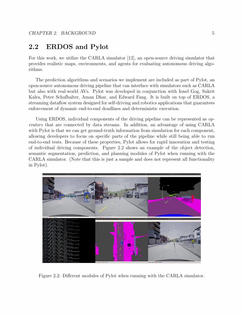
Using ERDOS, individual components of the driving pipeline can be represented as op-erators that are connected by data streams. In addition, an advantage of using CARLAwith Pylot is that we can get ground-truth information from simulation for each component,allowing developers to focus on specific parts of the pipeline while still being able to runend-to-end tests. Because of these properties, Pylot allows for rapid innovation and testingof individual driving components. Figure 2.2 shows an example of the object detection,semantic segmentation, prediction, and planning modules of Pylot when running with theCARLA simulator. (Note that this is just a sample and does not represent all functionalityin Pylot).

Figure 2.2: Different modules of Pylot when running with the CARLA simulator.

6

Chapter 3

Overview of Trajectory Prediction

We now focus on trajectory prediction, specifically for other vehicles in the environment.Pedestrian trajectory prediction is an equally important problem, but the two are oftenconsidered separately because pedestrians and vehicles have very different dynamics. Fur-thermore, it is easier to obtain high-quality, realistic data for vehicle trajectories than it isfor pedestrian trajectories.

Predicting future state is a common problem across many fields such as computer vision,so what makes vehicle trajectory prediction different from other types of prediction? Wecan incorporate knowledge about physical constraints on vehicle dynamics, but there is stillan extremely wide range of potential scenarios we may encounter. Classical approaches tothe prediction problem include physics-based models such as Kalman and switching Kalmanfilters [27], hidden Markov models, and Gaussian process prediction. Albrecht et al. [1] alsoprovide a comprehensive overview of non neural network-based methods, focusing on variousmodeling assumptions and modeling methods (e.g. policy reconstruction, graphical models).

However, like many other aspects of autonomous driving, trajectory prediction algorithmsmust deal with a long tail of unlikely but possible scenarios, so the ability to generalize froman incomprehensive dataset is key. This is one of the reasons why people have begun usingneural network-based approaches for the problem.

Applying this class of techniques to the trajectory prediction problem is fairly new. To thebest of our knowledge, Mozzafari et al. [26] provide the only survey of deep-learning basedapproaches for vehicle trajectory prediction. The authors structure their overview based onthe input representations (e.g. grid of the surrounding world from a bird’s eye view vs. rawsensor data) and output representations (intention-based, unimodal, multimodal predictions)that are common in the literature. They also discuss the prevalent network architecturesexisting approaches have tried, such as RNNs, CNNs, and Graph Neural Networks. In thenext section, we give a higher level overview of the state-of-the art approaches, with somediscussion of benefits and drawbacks of each category.

CHAPTER 3. OVERVIEW OF TRAJECTORY PREDICTION 7

3.1 Classification of Trajectory Prediction

Approaches

• Intention prediction models treat prediction as a classification problem of high-levelactions (intentions). For example, Luo et al. [8, 21] use end-to-end networks to jointlypredict agent intention with other aspects of the driving pipeline such as detection andtracking. Hu et al. [19] consider the highway lane-changing problem with intents fordifferent insertion areas.

While these methods allow for easily interpretable predictions, one drawback is thatthey require data to be manually labeled with intentions, which can be expensive andtime-consuming. In addition, intention prediction models do not output explicit tra-jectories by themselves, making it harder to incorporate their output into planningwithout some other auxiliary network or functionality. Today, many intention predic-tion models will do a combination of estimating the likelihood of each intention andgetting the most likely trajectory conditioned on that intention, or what Mozzafari etal. call “intention-based trajectory” predictions.

• Occupancy grid prediction methods [18, 17, 33, 25] assume we have a top-down dis-cretized grid map with occupancy probabilities for each location, and predict a similargrid of probabilities for each future time step up to some fixed horizon. Unlike intentionprediction, the output occupancy grids can directly be used for planning. However,these methods are significantly more memory-intensive, and don’t directly take advan-tage of the fact that we have distinct agents with physically-constrained dynamics.

• Game theoretic methods [14, 23, 22, 20] try to explicitly model interactions and col-laboration between multiple agents, e.g. by modeling the utility function of each agent(which can depend on other agents), then optimizing over possible actions. Thesemethods tend to become computationally intensive as the number of agents increase,because they consider the problem in its full generality. Therefore, they often still haveto make concessions with regards to modeling power.

For example, [14] decomposes the problem into two levels of planners: (i) a strategichigh-level planner that addresses fully coupled interaction using the Stackleberg leader-follower dynamic game, but with simplified dynamics, and (ii) a tactical planner thatconsiders accurate dynamics but with simplified interaction model, planning over ashorter (e.g. 1 s) duration and incorporating input from the high-level planner in theutility function.

• Graphical models influencing neural network design [9, 31, 32, 36]: These methodstypically assume the perception module is able to provide an accurate bird’s eye viewof its surroundings, along with perfect past trajectories of other agents. They thenuse various independence assumptions to tame the complexity of the problem, at the

CHAPTER 3. OVERVIEW OF TRAJECTORY PREDICTION 8

loss of some expressivity. We will discuss in more detail and evaluate three of thesenetworks in the next chapter.

3.2 Existing Metrics

Typically, trajectory prediction algorithms are evaluated on a static dataset of trajectories asopposed to in conjunction with a planning algorithm. In this static setting, a wide range ofother metrics have been proposed to evaluate the quality of trajectory prediction algorithmswhen applied to a static dataset of collected trajectories [5]. Two of the most commonlyused metrics for algorithms that predict a single trajectory are average displacementerror (ADE) and final displacement error (FDE).

Formally, given a sequence of past agent locations {x−t, . . . , x0} and some scene con-text φ, a trajectory prediction algorithm will output a sequence of predicted future states{x1, . . . , xT}. Denote the true agent trajectory by {x1, . . . , xT}. Then, average displacementerror is the Euclidean distance between the predicted and ground truth trajectory averagedover time, i.e. 1

T

∑Ti=1 ‖xi− xi‖2. Final displacement error is the Euclidean distance between

only the predicted and ground truth trajectory at time T , i.e. ‖xT − xT‖2.

The issue with ADE and FDE is that depending on the agent’s (hidden) goal, there couldbe several reasonable trajectories it can take. For example, at an intersection, we’d expectthere to be some non-zero probability that a vehicle could turn left, go straight, or turn right.ADE and FDE would both heavily penalize any single-trajectory predictor that happenedto choose the wrong mode, even if the predicted trajectory is reasonable given the intent.

Therefore, recent works [9, 32, 36] have used multimodal predictions in an attempt tocapture the inherent multimodality of the desired output. Consequently, these approachesare evaluated by taking the minimum ADE or minimum mean squared distance (minMSD)over a fixed number of joint predicted trajectories. As another example, the ongoing INTER-PRET prediction challenge, based off of the INTERACTION [38] dataset, uses this metricalong with ADE and FDE.

Finally, for models whose output defines a probability distribution over possible trajec-tories, another metric typically used is to evaluate the likelihood of the ground-truth futuretrajectory under this distribution. This metric captures how well the predicted distributioncovers all of the modes of the true distribution, but doesn’t penalize a model that assignshigh likelihood to trajectories that are in reality unlikely.

9

Chapter 4

Experiments

4.1 Simulation Setup and Algorithms

We consider four different trajectory prediction models, a baseline linear regression modeland three neural-network based trajectory prediction models that fall under the last categorydescribed in the previous chapter (graphical models influencing neural network design). Wefirst describe the defining attributes of each method.

1. Linear prediction assumes each agent will travel at a constant velocity, and uses linearregression on past agent locations to predict its future locations.

2. R2P2 [31] is a state-of-the-art single-agent trajectory forecasting model. It learns adistribution over potential future trajectories that is parameterized by a one-step policyusing a gated recurrent unit (GRU), and attempts to optimize for both quality anddiversity of samples.

To extend R2P2 to the multi-agent setting, we run R2P2 on every agent within aspecified prediction radius, rotating the scene context and past trajectories of otheragents to the coordinate frame of the agent we are making predictions for. We referto this version of R2P2 as R2P2-MA (R2P2-MultiAgent). The computations for eachagent are independent and can therefore be batched.

3. Multipath [9] predicts a mixture of Gaussians distribution for agent locations at eachtime step. First, K anchor trajectories are derived from the training data, eitherthrough K-means clustering with Euclidean distance or by sampling fixed trajectories.The number of anchors K can vary depending on the problem. Then, the state distri-bution at each time step is conditionally Gaussian with learned mean and covariance,and independent of the distribution at other time steps given an anchor trajectory.

For its network architecture, Multipath first uses a lightweight scene-level network (inour implementation, we used a depth-wise thinned out version of Resnet-18) to obtain

CHAPTER 4. EXPERIMENTS 10

a useful feature representation of the scene. Then, it applies a smaller network onthe relevant features for each agent that outputs predictions, represented as deviationsfrom each anchor trajectory, as well as a probability distribution over anchors. Becausethe same network is used for each agent, per-agent computation can also be batchedand both stages of the network are fairly fast.

4. Multiple Futures Prediction (MFP) [36] includes an attention-based mechanism tojointly model agent behavior, in addition to the initial feature processing stages thatare fairly similar to those in the other works. The network architecture also givesthe flexibility of varying the number of discrete latent modes used for the outputtedprediction distribution.

With the exception of linear prediction, which doesn’t require any training, all modelsdescribed were trained on the PRECOG dataset. This dataset consists of roughly 60000training samples of driving behavior in Town01 of the CARLA simulator, with each sampleconsisting of the ego-vehicle’s current LIDAR observation, as well as two seconds of pasttrajectory history and four seconds of future trajectory for each agent.

We chose these models in order to represent some of the major classes of neural-networkbased approaches for trajectory prediction. Linear prediction is an extremely fast baseline,which while clearly not applicable in all contexts, has its use cases in niche contexts. R2P2was chosen as a representative of taking a single-agent forecasting model and naıvely extend-ing it to the multiagent setting. Multipath was chosen as a multi-agent forecasting modelthat is very fast because of the independence assumptions and lightweight architecture that ituses. Finally, MFP was chosen because it is the current state-of-the art in vehicle trajectoryprediction.

We simulated the scenarios using CARLA 0.9.8’s scenario runner module [7]. CARLAprovides two modes of execution: (i) Synchronous, where the simulator allows instantaneousapplication of control commands by pausing the simulator time after sending sensor inputs tothe client, and (ii) Asynchronous, where the simulator keeps moving time forward and appliesthe control command when the client finishes execution. While CARLA’s asynchronous modeallows us to observe the effects of the runtime of Pylot, it does not provide us with the abilityto apply a control command at a specific simulation time.

To better control the effects of runtime on the simulation, we run CARLA in synchronousmode with a high frequency of 200Hz, and attach a synchronizer operator between the controlmodule and the simulator. This synchronizer tracks the runtime of the pipeline for eachsensor input, and buffers the generated control command until the simulation time is greaterthan or equal to the sum of the sensor input time and the runtime of the pipeline. Thisallows us to simulate running the pipeline asynchronously, but with the ability to manage

CHAPTER 4. EXPERIMENTS 11

when control commands are applied that CARLA’s asynchronous mode does not provide.We call this mode of execution pseudo-asynchronous mode.

4.2 Factors Affecting Prediction Quality

Algorithm Runtime

Table 4.1 shows the minMSD metrics on the Town01 test portion of the PRECOG datasetfor the above approaches. The minMSD was taken over 12 sets of sampled joint trajectories(this metric becomes just the MSD for the linear predictor because it gives a deterministicoutput). MFP-4 represents running MFP with four latent modes.

Approach minMSD12

Linear 1.10R2P2-MA 0.77MultiPath 0.68

MFP-4 0.28

Table 4.1: minMSD values for several prediction networks.

From this table, our initial impression might be that we should always run MFP-4,because it gives us the best minMSD. However, we need to take into account the runtimesof each method. To see why, consider a scenario in which a vehicle approaches a four wayintersection at the same time as our autonomous vehicle. We may initially believe thatthe vehicle is going straight. However, a slight turn or signal would indicate to a humandriver that the vehicle is about to turn. Taking too long to run prediction may mean thatour autonomous vehicle misses this signal, and continues thinking the other vehicle will gostraight.

In addition, if we take too long to perform prediction (especially at high speeds) theenvironment will have already changed drastically by the time we receive those predictions.In this case, we might as well get new sensor readings and use those instead of runningprediction on old data.

We confirm this intuition in a four-way intersection scenario using the CARLA scenariorunner. As depicted in Figure 4.1, our autonomous vehicle approaches a four-way intersectionat the same time as a vehicle on the road perpendicular to us. However, the other vehiclefails to stop and speeds through the intersection, so we must either emergency brake orswerve to avoid an accident. Note that prediction is necessary for this scenario, as we needto know sufficiently early that the other vehicle is going too fast and that we may need toslow down.

CHAPTER 4. EXPERIMENTS 12

Figure 4.1: Four-way intersection collision avoidance scenario from a bird’s-eye view. Darkgreen dots represent past trajectories, and light green dots represent predictions. The ego-vehicle is the bottom one.

Figure 4.2: Due to our sampling strategy, R2P2 can sometimes be unstable, but this did notaffect driving performance as the ego-vehicle has to emergency stop at that distance.

CHAPTER 4. EXPERIMENTS 13

For simplicity, we provide the autonomous vehicle with access to perfect past tracks ofthe other vehicle once it comes in view, as well as LIDAR readings. In addition, for eachof the neural network-based planners, we sample from the predicted distribution of futuretrajectories and use that as our prediction. Although this does not take into account the fulltrajectory distribution, this naıve sampling suffices for all predictors for the purposes of ourscenario. This was somewhat unstable in the case of R2P2-MA as shown in Figure 4.2, as wewould predict going straight at some time steps and predict turns at subsequent time steps,but this behavior did not interfere with our results. As stated earlier, we run this scenarioin pseudo-asynchronous mode.

We use an implementation of the Frenet planner, as it performs consistently and is ableto swerve for obstacle avoidance, although it does require a relatively long runtime. Inthis situation, the linear predictor is able to avoid the collision by swerving slightly to buytime and then continuing along its path, but using R2P2 can sometimes result in collisionsbecause of the increased runtime (depending on runtime variability in both R2P2 and theFrenet planner).

Figure 4.3: Average runtimes of our four models in the scenario. All runtimes are measuredwith a batch size of 1; we can’t batch predictions in the auto-driving setting, as data comesin an online fashion.

These results make sense given the runtime of our four models as shown in Figure 4.3.We observe that there is roughly a 150 ms difference between the slowest and fastest models,which means that when traveling at 16 m/s as in our scenario, there is roughly a 0.15∗16 = 2.4meter difference between when the planner is able to react when using the different predictors.This is a relatively small but still significant distance, and we suspect that when coupledwith runtime differences incurred when switching components in other parts of the pipeline,this phenomenon will only be exacerbated.

We also experimented with using a simple waypoint planner, which follows a list ofwaypoints given to it and emergency brakes when an obstacle impedes its path (rather than

CHAPTER 4. EXPERIMENTS 14

swerving). After searching over a range of speeds and distances for both vehicles, we didnot find a configuration for which both using the waypoint planner with the linear predictorworked, and using the waypoint planner with R2P2-MA caused a collision. This is becausewithout swerving or other forms of obstacle avoidance, there was no speed that was highenough to create a significant distance difference between the different predictors, yet lowenough such that we could brake in time to avoid the collision. However, one could arguethat using the linear predictor is still better because it lessens the speed at collision time,making the ride safer.

Of course, a linear predictor is not sufficient in all scenarios. We can consider the samescenario as above, except that the other vehicle comes from the left side of the intersectionand decides to turn right. In this case, the behavior of the other vehicle should not affectour plan. However, the linear predictor is overcautious and predicts the other vehicle maygo straight through the intersection or even drive straight towards us as it begins to turn,leading to unneccessary braking and an uncomfortable ride.

Finally, when is MFP preferred over R2P2-MA and Multipath? MFP has the ability tomodel interactions in more complex driving scenarios. In contrast, because R2P2-MA andMultiPath generate predictions on a per-agent basis independently, they would not sufficefor these scenarios, and the minMSD metrics are indicative of this phenomenon. MFP wouldbe especially effective in these crowded scenes when we are driving at slower speeds and havemore time to react.

Environment Complexity

Having established that runtime should be considered when evaluating prediction models,we now discuss the effects of different aspects of the environment on each models’ runtime.First, we note that linear regression is extremely fast (no more than a few milliseconds) forany reasonable prediction horizon and environment that we would encounter.

Many prediction networks, including R2P2-MA and MFP, utilize recurrent neural net-works in their architecture, which perform inherently sequential computation. Consequently,in situations such as highway driving which involve faster speeds and longer braking distancesfor which we need longer prediction horizons, these models have increased runtime. FigureFigure 4.4 shows the runtime of R2P2-MA and MFP-1 with different prediction horizonsand one other agent in the scene.

In contrast, the runtime of Multipath has little dependence on the prediction horizon.This is because the second stage of the network architecture is fully convolutional, so batchingallows runtimes to stay roughly the same.

With regards to the number of agents we perform predictions for, we found that onlyMFP’s runtime scales with the number of agents. For both R2P2-MA and Multipath, the

CHAPTER 4. EXPERIMENTS 15

1 2 3 4 5Prediction horizon [s]

0

50

100

150

200

250

Run

time

[ms]

R2P2-MAMFP

Figure 4.4: Prediction runtime can increase as prediction horizon increases.

per-agent computation can be performed independently and batched. However, because ofthe attention mechanism of MFP, we found that with an increased number of agents itsruntime also increased.

Perhaps surprisingly, none of these methods are affected by the number of static obstaclesin the scene, as they take in scene context as a LIDAR point cloud (or potentially an imageof fixed size) and apply some form of a convolutional feature extractor.

Frequency of Predictions

A typical AV is equipped with a dozen cameras, several LIDARs, and radars, which collec-tively generate 1–2 GB/s of data. This data must be processed by the pipeline to reach acontrol decision, which needs to be made faster than the typical human reaction time. Withso many components in the pipeline and relatively insufficient computation power on today’sautonomous vehicles [29], prioritization of computation resources is essential.

In addition to switching between components along the runtime-accuracy tradeoff curveas in the previous section, in some situations we could run certain components less often ifthey are not as vital to the end-to-end performance of the pipeline in the current context.

For example, it is not always necessary to run neural network based prediction for everyframe. To see this, we consider the following experiment setup, as shown in Figure 4.5. Theego-agent is driving down a straight road, with a static pedestrian at the end of it. We havea simple module that tells us whether or not any agents could feasibly affect our trajectory.For example, if the object tracker tells us that all nearby vehicles are oriented away from us,and physical constraints mean that they have very little chance to impact our ego-vehicle’splan, we don’t need to run prediction until we receive a new tracked object from the objecttracking module.

CHAPTER 4. EXPERIMENTS 16

Figure 4.5: The ego-vehicle can choose not to run prediction if no vehicles are physicallyable to collide with it in the near future, and allocate more time to object detection.

We saw in Figure 4.3 that not running one of the computationally expensive predictionmodules could save us roughly 150 ms of runtime per frame. We can invest this freed-uptime into improving the accuracy of other modules in our pipeline, such as object detection.Table 4.2 shows the runtimes of various EfficientDet models [35], as well as what distancewe can be at while still detecting a static pedestrian using each version of EfficientDet inthe CARLA scenario runner. EfficientDet is a family of state-of-the-art single-stage objectdetectors that give us nice tradeoffs in runtime and accuracy, which is why we discuss ithere. The extra time gained from not having to run prediction allows us to use a higher-accuracy EfficientDet model while having comparable response times (e.g. switch from usingEfficientDet-d2 to EfficientDet-d6), allowing us to detect the obstacle earlier and stop in time.In addition, not outputting predictions at every time step has the added advantage of givingmore realistic and stable predictions [36].

EfficientDet Model Distance Detected (m) Runtime(ms)d1 7.31 12d2 12.42 16d3 16.93 23d4 22.97 37d5 37.00 65d6 48.39 128d7 49.05 232

Table 4.2: Detection distances and runtimes for different EfficientDet models.

CHAPTER 4. EXPERIMENTS 17

Probabilities assigned to each predicted trajectory

We saw in Section 3.2 that metrics such as minMSD and minADE were introduced to takeinto account the fact that predictions should inherently be multimodal. However, thesemetrics don’t take into account the probabilities assigned to each sampled trajectory.

For example, in Figure 4.6, we can consider two predictors which output the same threepaths (turning left, slowing down, turning right), but with different probability distributions,e.g. [0.8, 0.1, 0.1] and [0.1, 0.8, 0.1]. If the ground-truth path is one of these three paths, bothpredictors would have a minMSD and minADE of zero. However, it makes a big differenceto the planning module if we know whether this vehicle is more likely to turn left or slowdown.

Figure 4.6: Predicting correct paths must also come with predicting correct probabilities.

Therefore, metrics such as minMSD and minADE can be more useful than single-trajectoryMSD and ADE, but they do not necessarily correlate with good planning performance.

18

Chapter 5

Conclusion and Future Work

Currently, trajectory prediction is one of the major hurdles remaining in order to achieve safeand reliable autonomous driving. There have been many proposed metrics for evaluatingthe quality of predictions on static datasets. However, trajectory prediction for autonomousdriving inherently must run in real-time, in conjunction with other components of the driv-ing pipeline such as planning. We have discussed why factors such as algorithm runtime,environment complexity, and frequency of predictions should also be taken into accountwhen evaluating a prediction algorithm. To do this, we implemented several state-of-the-artprediction models and evaluated their behavior in a realistic simulation.

Future work could involve considering trajectory prediction for pedestrians as well. Oneadditional challenge for pedestrians is that they have less consistent dynamics models, aswell as different physical constraints on the set of feasible paths. We could also incorporatereal data on vehicle signalling lights and horns, as human drivers depend a lot on thesecues for making predictions. Also, it would be useful to evaluate algorithms which jointlyperform planning and prediction. In reality, the two modules cannot be considered separately,as the decision of the ego-vehicle matters for the predicted trajectories of other vehicles.For example, at a four-way intersection, nudging forward can signal to other cars at theintersection that you plan to cross, so they are more likely to cede the right of way. This isanother aspect of prediction quality that cannot be evaluated by a static dataset.

Another natural extension to this work would be to consider planners that leverage theinherent uncertainty of the predictions, taking into account the full distribution of trajectoriesproduced by the model. A naıve approach would be to sample multiple trajectories from thepredicted distribution and consider all of the corresponding locations as being occupied, butwe found that this led to an overcautious agent, an example of the freezing robot problem.We could also consider probabilistic planners, which treat the prediction problem as a MarkovDecision Process (MDP). These planners account for action and environment uncertainty,and they would allow for tighter integration between the planning and prediction modules.

19

Bibliography

[1] Stefano V Albrecht and Peter Stone. “Autonomous agents modelling other agents:A comprehensive survey and open problems”. In: Artificial Intelligence 258 (2018),pp. 66–95.

[2] Autoware. Autoware User’s Manual - Document Version 1.1. url: https://github.com/CPFL/Autoware-Manuals/blob/master/en/Autoware_UsersManual_v1.1.md.

[3] Claudine Badue et al. “Self-Driving Cars: A Survey”. In: CoRR abs/1901.04407 (2019).arXiv: 1901.04407. url: http://arxiv.org/abs/1901.04407.

[4] Baidu. Apollo 3.0 Software Architecture. url: https://github.com/ApolloAuto/apollo/blob/master/docs/specs/Apollo_3.0_Software_Architecture.md.

[5] Philippe Besse et al. Review and Perspective for Distance Based Trajectory Clustering.2015. arXiv: 1508.04904 [stat.ML].

[6] Alex Bewley et al. “Simple online and realtime tracking”. In: 2016 IEEE InternationalConference on Image Processing (ICIP). IEEE. 2016, pp. 3464–3468.

[7] CARLA 0.9.8. https://carla.org/2020/03/09/release-0.9.8/.

[8] Sergio Casas, Wenjie Luo, and Raquel Urtasun. “Intentnet: Learning to predict inten-tion from raw sensor data”. In: Conference on Robot Learning. 2018, pp. 947–956.

[9] Yuning Chai et al. MultiPath: Multiple Probabilistic Anchor Trajectory Hypotheses forBehavior Prediction. 2019. arXiv: 1910.05449 [cs.LG].

[10] Henry Claypool, Amitai Bin-Nun, and Jeffrey Gerlach. “Self-driving cars: The impacton people with disabilities”. In: Newton, MA: Ruderman Family Foundation (2017).

[11] Felipe Codevilla et al. “End-to-end driving via conditional imitation learning”. In: 2018IEEE International Conference on Robotics and Automation (ICRA). IEEE. 2018,pp. 1–9.

[12] Alexey Dosovitskiy et al. “CARLA: An Open Urban Driving Simulator”. In: arXivpreprint arXiv:1711.03938 (2017).

[13] ERDOS. https://github.com/erdos-project.

BIBLIOGRAPHY 20

[14] Jaime F Fisac et al. “Hierarchical game-theoretic planning for autonomous vehicles”.In: 2019 International Conference on Robotics and Automation (ICRA). IEEE. 2019,pp. 9590–9596.

[15] General Motors. 2018 Self-driving safety report. url: https://www.gm.com/content/dam/company/docs/us/en/gmcom/gmsafetyreport.pdf.

[16] Hars, Alexander. Top misconceptions of autonomous cars and self-driving vehicles.http://www.inventivio.com/innovationbriefs/2016-09/Top-misconceptions-

of-self-driving-cars.pdf.

[17] Stefan Hoermann, Martin Bach, and Klaus Dietmayer. “Dynamic occupancy gridprediction for urban autonomous driving: A deep learning approach with fully auto-matic labeling”. In: 2018 IEEE International Conference on Robotics and Automation(ICRA). IEEE. 2018, pp. 2056–2063.

[18] Joey Hong, Benjamin Sapp, and James Philbin. “Rules of the road: Predicting drivingbehavior with a convolutional model of semantic interactions”. In: Proceedings of theIEEE Conference on Computer Vision and Pattern Recognition. 2019, pp. 8454–8462.

[19] Yeping Hu, Wei Zhan, and Masayoshi Tomizuka. “Probabilistic prediction of vehiclesemantic intention and motion”. In: 2018 IEEE Intelligent Vehicles Symposium (IV).IEEE. 2018, pp. 307–313.

[20] Daphne Koller and Brian Milch. “Multi-agent influence diagrams for representing andsolving games”. In: Games and economic behavior 45.1 (2003), pp. 181–221.

[21] Wenjie Luo, Bin Yang, and Raquel Urtasun. “Fast and furious: Real time end-to-end 3d detection, tracking and motion forecasting with a single convolutional net”.In: Proceedings of the IEEE conference on Computer Vision and Pattern Recognition.2018, pp. 3569–3577.

[22] Wei-Chiu Ma et al. “A gametheoretic approach to multi-pedestrian activity forecast-ing”. In: arXiv preprint arXiv:1604.01431 2 (2016).

[23] Wei-Chiu Ma et al. “Forecasting interactive dynamics of pedestrians with fictitiousplay”. In: Proceedings of the IEEE Conference on Computer Vision and Pattern Recog-nition. 2017, pp. 774–782.

[24] Michele Bertoncello, and Dominik Wee. Ten ways autonomous driving could redefinethe automotive world. https://www.mckinsey.com/industries/automotive-and-assembly/our-insights/ten-ways-autonomous-driving-could-redefine-the-

automotive-world.

[25] Nima Mohajerin and Mohsen Rohani. “Multi-step prediction of occupancy grid mapswith recurrent neural networks”. In: Proceedings of the IEEE Conference on ComputerVision and Pattern Recognition. 2019, pp. 10600–10608.

[26] Sajjad Mozaffari et al. “Deep Learning-based Vehicle Behaviour Prediction For Au-tonomous Driving Applications: A Review”. In: arXiv preprint arXiv:1912.11676 (2019).

BIBLIOGRAPHY 21

[27] Kevin P Murphy. “Switching kalman filters”. In: (1998).

[28] National Highway Traffic Safety Administration. Traffic Safety Facts (2017 Data).https://crashstats.nhtsa.dot.gov/Api/Public/ViewPublication/812687.

[29] NVIDIA. 2018 Self-driving safety report. https://www.nvidia.com/content/dam/en-zz/Solutions/self-driving-cars/safety-report/NVIDIA-Self-Driving-

Safety-Report-2018.pdf.

[30] Brian Paden et al. “A survey of motion planning and control techniques for self-drivingurban vehicles”. In: IEEE Transactions on intelligent vehicles 1.1 (2016), pp. 33–55.

[31] Nicholas Rhinehart, Kris M Kitani, and Paul Vernaza. “R2p2: A reparameterized push-forward policy for diverse, precise generative path forecasting”. In: Proceedings of theEuropean Conference on Computer Vision (ECCV). 2018, pp. 772–788.

[32] Nicholas Rhinehart et al. “Precog: Prediction conditioned on goals in visual multi-agent settings”. In: Proceedings of the IEEE International Conference on ComputerVision. 2019, pp. 2821–2830.

[33] Marcel Schreiber, Stefan Hoermann, and Klaus Dietmayer. “Long-term occupancygrid prediction using recurrent neural networks”. In: 2019 International Conferenceon Robotics and Automation (ICRA). IEEE. 2019, pp. 9299–9305.

[34] State of California Department of Motor Vehicles. Autonomous Vehicle DisengagementReports 2018. https://www.dmv.ca.gov/portal/dmv/detail/vr/autonomous/disengagement_report_2019.

[35] Mingxing Tan, Ruoming Pang, and Quoc V Le. “Efficientdet: Scalable and efficientobject detection”. In: arXiv preprint arXiv:1911.09070 (2019).

[36] Yichuan Charlie Tang and Ruslan Salakhutdinov. Multiple Futures Prediction. 2019.arXiv: 1911.00997 [cs.LG].

[37] M. Werling et al. “Optimal trajectory generation for dynamic street scenarios in aFrenet Frame”. In: 2010 IEEE International Conference on Robotics and Automation.2010, pp. 987–993.

[38] Wei Zhan et al. INTERACTION Dataset: An INTERnational, Adversarial and Coop-erative moTION Dataset in Interactive Driving Scenarios with Semantic Maps. 2019.arXiv: 1910.03088 [cs.RO].