CH.7 Sampling Distributions and Point Estimation of … · 20 7-3 General Concepts of Point...
48
1 CH.7 Sampling Distributions and Point Estimation of Parameters • Introduction – Parameter estimation, sampling distribution, statistic, point estimator, point estimate • Sampling distribution and the Central Limit Theorem • General Concepts of Point Estimation – Unbiased estimators – Variance of a point estimator – Standard error of an estimator – Mean squared error of an estimator • Methods of point estimation – Method of moments – Method of maximum likelihood
Transcript of CH.7 Sampling Distributions and Point Estimation of … · 20 7-3 General Concepts of Point...
1
CH.7 Sampling Distributions andPoint Estimation of Parameters
• Introduction– Parameter estimation, sampling distribution, statistic, point estimator,
point estimate• Sampling distribution and the Central Limit Theorem• General Concepts of Point Estimation
– Unbiased estimators– Variance of a point estimator– Standard error of an estimator– Mean squared error of an estimator
• Methods of point estimation– Method of moments– Method of maximum likelihood
2
7-1 Introduction
•The field of statistical inference consists of those methods used to make decisions or to draw conclusions about a population.
• These methods utilize the information contained in a sample from the population in drawing conclusions.
• Statistical inference may be divided into two major areas:
• Parameter estimation
• Hypothesis testing
3
7-1 Introduction
Parameter estimation examples
•Estimate the mean fill volume of soft drink cans: Soft drink cansare filled by automated filling machines. The fill volume mayvary because of differences in soft drinks, automated machines, and measurement procedures.
• Estimate the mean diameter of bottle openings of a specificbottle manufactured in a plant: The diameter of bottle openingsmay vary because of machines, molds and measurements.

4
7-1 Introduction
Hypothesis testing example
•2 machine types are used for filling soft drink cans: m1 and m2
• You have a hypothesis that m1 results in larger fill volume of soft drink cans than does m2.
•Construct the statistical hypothesis as follows:
• the mean fill volume using machime m1 is larger than themean fill volume using machine m2.
• Try to draw conclusions about a stated hypothesis.
5
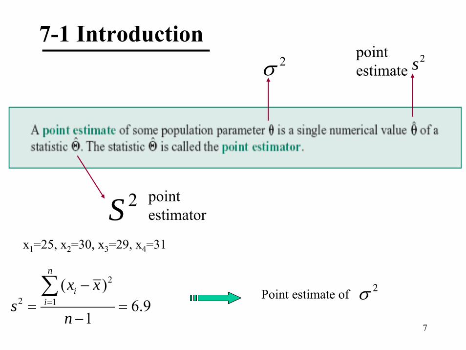
Definition
7-1 Introduction
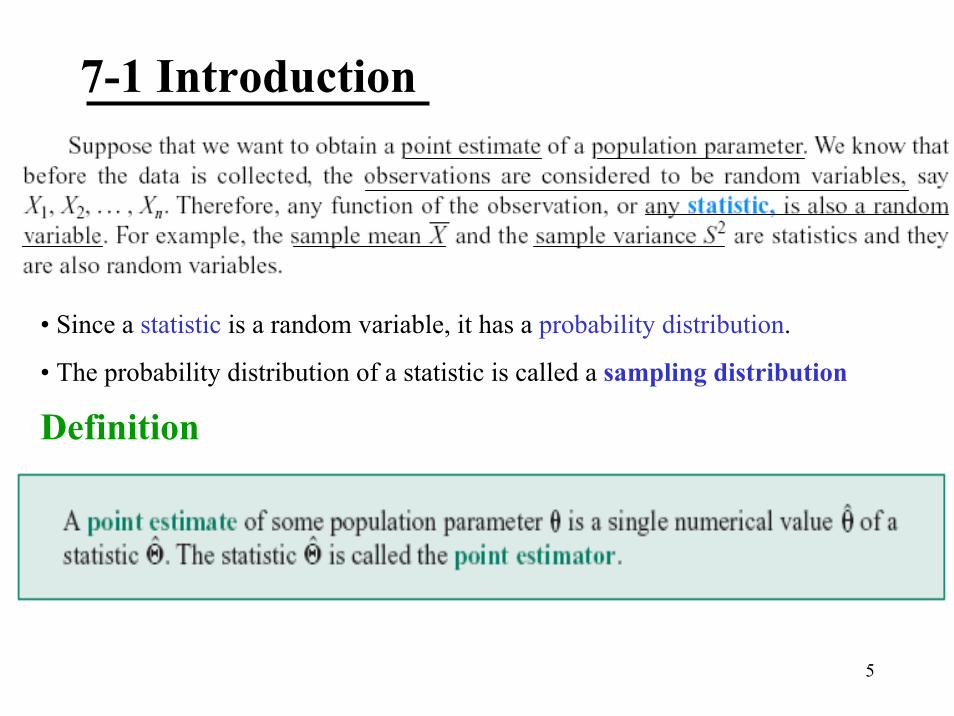
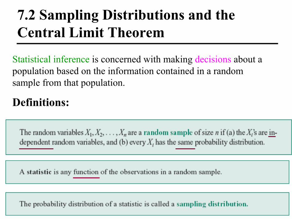
• Since a statistic is a random variable, it has a probability distribution.
• The probability distribution of a statistic is called a sampling distribution
6
7-1 Introduction
μ
xμ
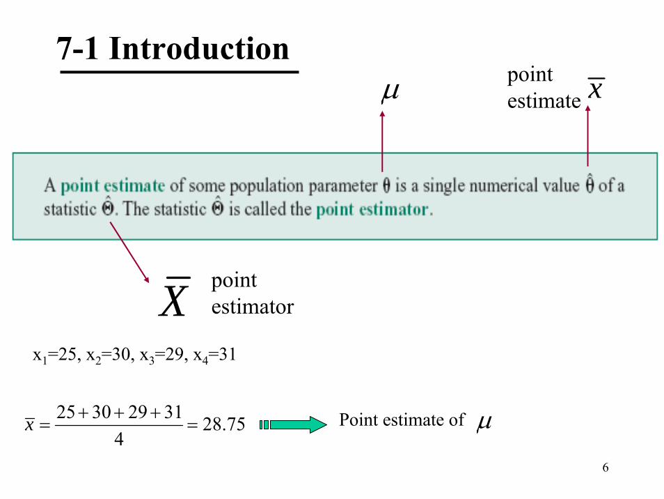
Xx1=25, x2=30, x3=29, x4=31
25 30 29 31 28.754
x + + += = Point estimate of μ
pointestimate
pointestimator
7
7-1 Introduction
μ
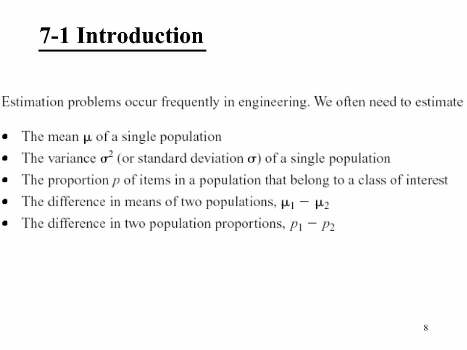
2s2σ
2Sx1=25, x2=30, x3=29, x4=31
2
2 1( )
6.91
n
ii
x xs
n=
−= =
−
∑ Point estimate of 2σ
pointestimate
pointestimator
8
7-1 Introduction
9
7-1 Introduction
10
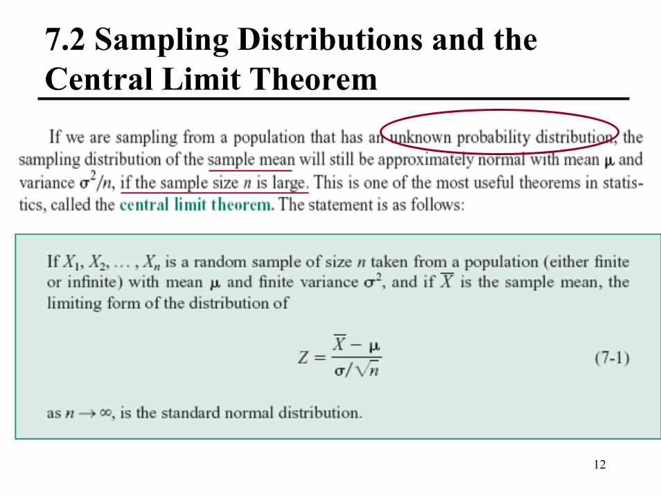
7.2 Sampling Distributions and the Central Limit Theorem
Statistical inference is concerned with making decisions about a population based on the information contained in a random sample from that population.
Definitions:

11
7.2 Sampling Distributions and the Central Limit Theorem
• The probability distribution of is called the sampling distribution of mean.• Suppose that a random sample of size n is taken from a normal population with mean and
variance .
• Each observation X1, X2,…,Xn is normally and independently distributed with mean andvariance
• Linear functions of independent normally distributed random variables are also normallydistributed. (Reproductive property of Normal Distr.)
• The sample mean has a normal distribution
• with mean
• and variance
Xμ
2σμ
2σ
1 2 ... nX X XXn
+ + +=
...x n
μ μ μμ μ+ + += =
2 2 2 22
2
...X n n
σ σ σ σσ + + += =
2
,X Nnσμ
⎛ ⎞⎜ ⎟⎝ ⎠
∼
12
7.2 Sampling Distributions and the Central Limit Theorem
13
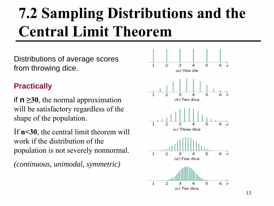
7.2 Sampling Distributions and the Central Limit Theorem
Distributions of average scores from throwing dice.
Practically
if n ≥30, the normal approximationwill be satisfactory regardless of theshape of the population.
İf n<30, the central limit theorem willwork if the distribution of thepopulation is not severely nonnormal.
(continuous, unimodal, symmetric)

14
7.2 Sampling Distributions and the Central Limit TheoremExample 7-1
15
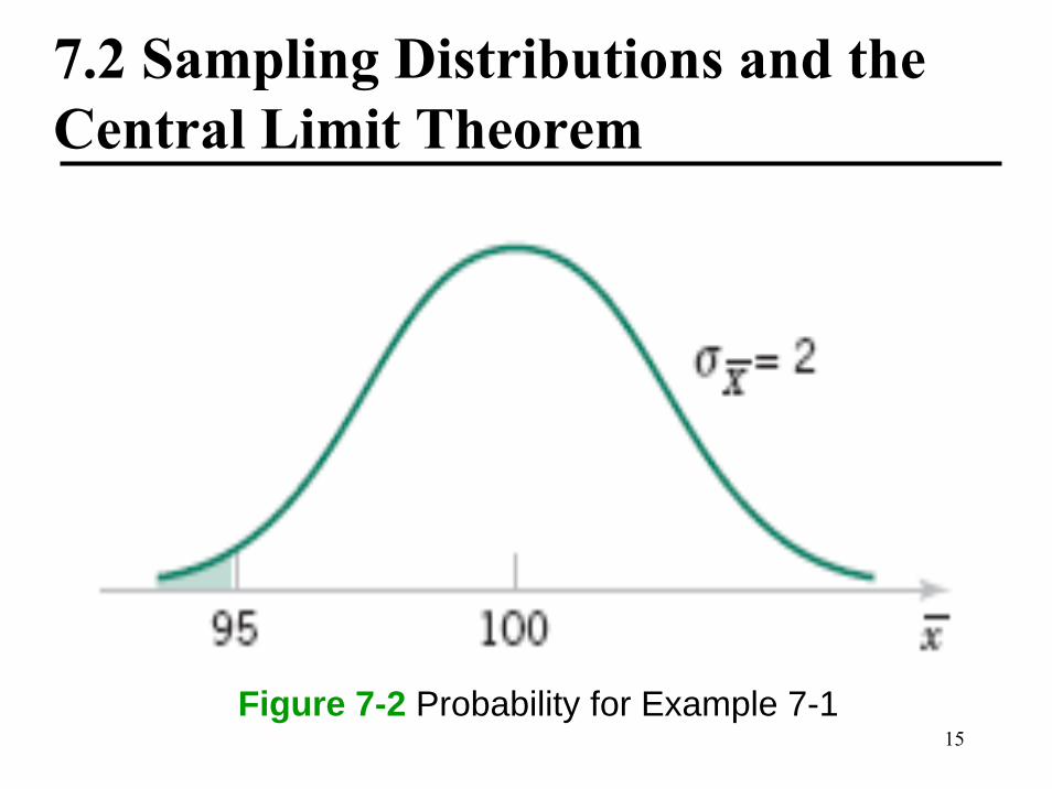
7.2 Sampling Distributions and the Central Limit Theorem
Figure 7-2 Probability for Example 7-1
16
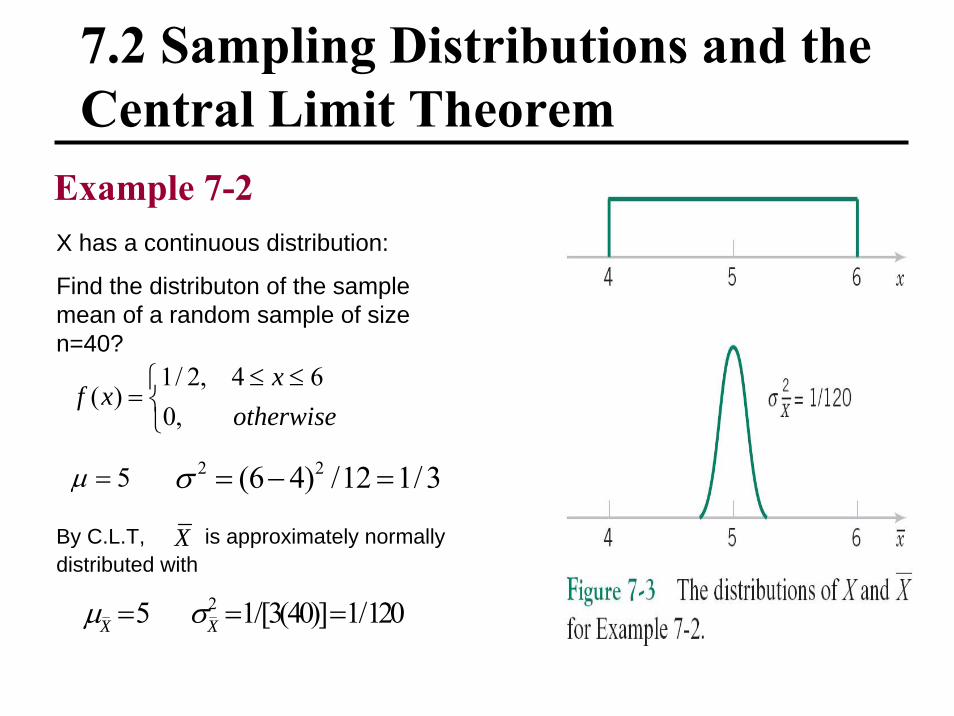
7.2 Sampling Distributions and the Central Limit Theorem
X has a continuous distribution:
Find the distributon of the samplemean of a random sample of size n=40?
Example 7-2
1/ 2, 4 6( )
0,x
f xotherwise≤ ≤⎧
= ⎨⎩
5μ = 2 2(6 4) /12 1/3σ = − =
By C.L.T, is approximately normallydistributed with
X
25 1/[3(40)] 1/120X Xμ σ= = =
17
7.2 Sampling Distributions and the Central Limit Theorem
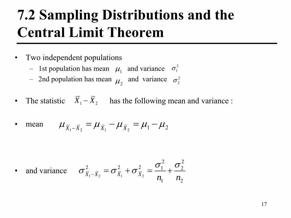
• Two independent populations– 1st population has mean and variance– 2nd population has mean and variance
• The statistic has the following mean and variance :
• mean
• and variance
1 2X X−
1 2 1 2 1 2X X X Xμ μ μ μ μ− = − = −
1 2 1 2
2 22 2 2 1 2
1 2X X X X n n
σ σσ σ σ− = + = +
1μ
2μ
21σ
22σ

18
7.2 Sampling Distributions and the Central Limit Theorem
Approximate Sampling Distribution of a Difference in Sample Means

19
7.2 Sampling Distributions and the Central Limit Theorem Ex.7-3
• Two independent and approximately normal populations– X1: life of a component with old process =5000 =40– X2: life of a component with improved process =5050 =30
• n1=16 , n2=25• What is the probability that the difference in the two sample meansis at least 25 hours?
2 1X X−
2 1 2 150X X X Xμ μ μ− = − =
2 1 2 1
2 2 2 136X X X Xσ σ σ− = + =
1μ
2μ1σ
2σ
1 1
2 22 1
11
405000 10016X X n
σμ μ σ= = = = =
2 2
2 22 2
22
305050 3625X X n
σμ μ σ= = = = =
( )2 1
2 1
2 1
25 25 50( 25) 2.14 0.9838136
X X
X X
P X X P Z P Z P Zμ
σ−
−
⎛ ⎞− −⎛ ⎞− ≥ = ≥ = ≥ = ≥ − =⎜ ⎟ ⎜ ⎟⎜ ⎟ ⎝ ⎠⎝ ⎠
20
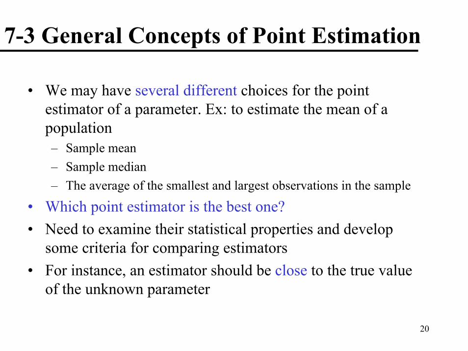
7-3 General Concepts of Point Estimation
• We may have several different choices for the pointestimator of a parameter. Ex: to estimate the mean of a population– Sample mean– Sample median– The average of the smallest and largest observations in the sample
• Which point estimator is the best one?• Need to examine their statistical properties and develop
some criteria for comparing estimators• For instance, an estimator should be close to the true value
of the unknown parameter
21
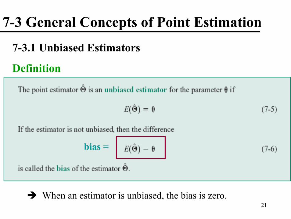
7-3 General Concepts of Point Estimation
7-3.1 Unbiased Estimators
Definition
When an estimator is unbiased, the bias is zero.
bias =
22
7-3 General Concepts of Point Estimation
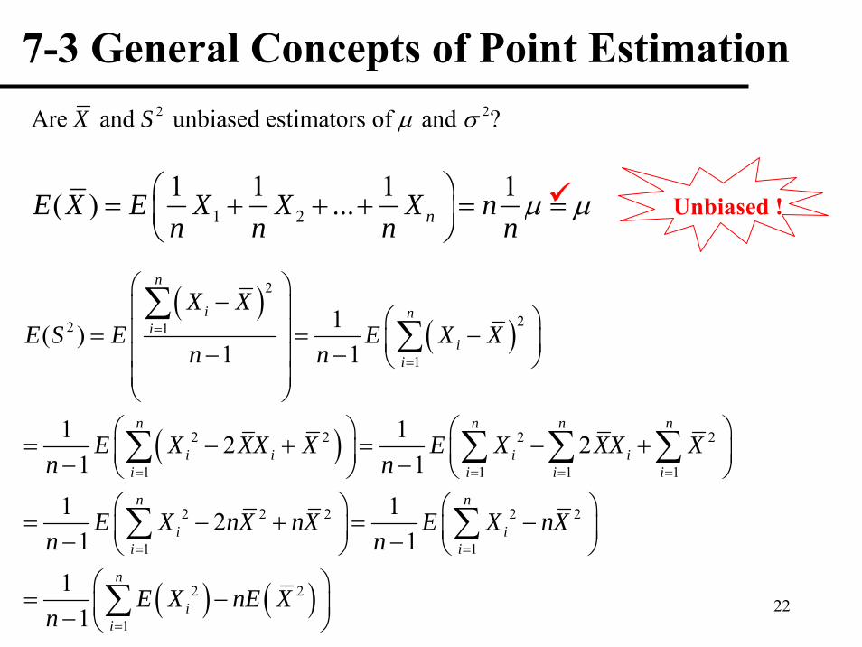
1 21 1 1 1( ) ... nE X E X X X nn n n n
μ μ⎛ ⎞= + + + = =⎜ ⎟⎝ ⎠
2 2Are and unbiased estimators of and ?X S μ σ
Unbiased !
( )( )
( )
( ) ( )
2
22 1
1
2 2 2 2
1 1 1 1
2 2 2 2 2
1 1
2 2
1
1( )1 1
1 12 21 1
1 121 1
11
n
i ni
ii
n n n n
i i i ii i i i
n n
i ii i
n
ii
X XE S E E X X
n n
E X XX X E X XX Xn n
E X nX nX E X nXn n
E X nE Xn
=
=
= = = =
= =
=
⎛ ⎞−⎜ ⎟ ⎛ ⎞⎜ ⎟= = −⎜ ⎟− −⎜ ⎟ ⎝ ⎠⎜ ⎟⎝ ⎠
⎛ ⎞ ⎛ ⎞= − + = − +⎜ ⎟ ⎜ ⎟− −⎝ ⎠ ⎝ ⎠⎛ ⎞ ⎛ ⎞
= − + = −⎜ ⎟ ⎜ ⎟− −⎝ ⎠ ⎝ ⎠⎛ ⎞= −⎜ ⎟− ⎝ ⎠
∑∑
∑ ∑ ∑ ∑
∑ ∑
∑
23
7-3 General Concepts of Point Estimation
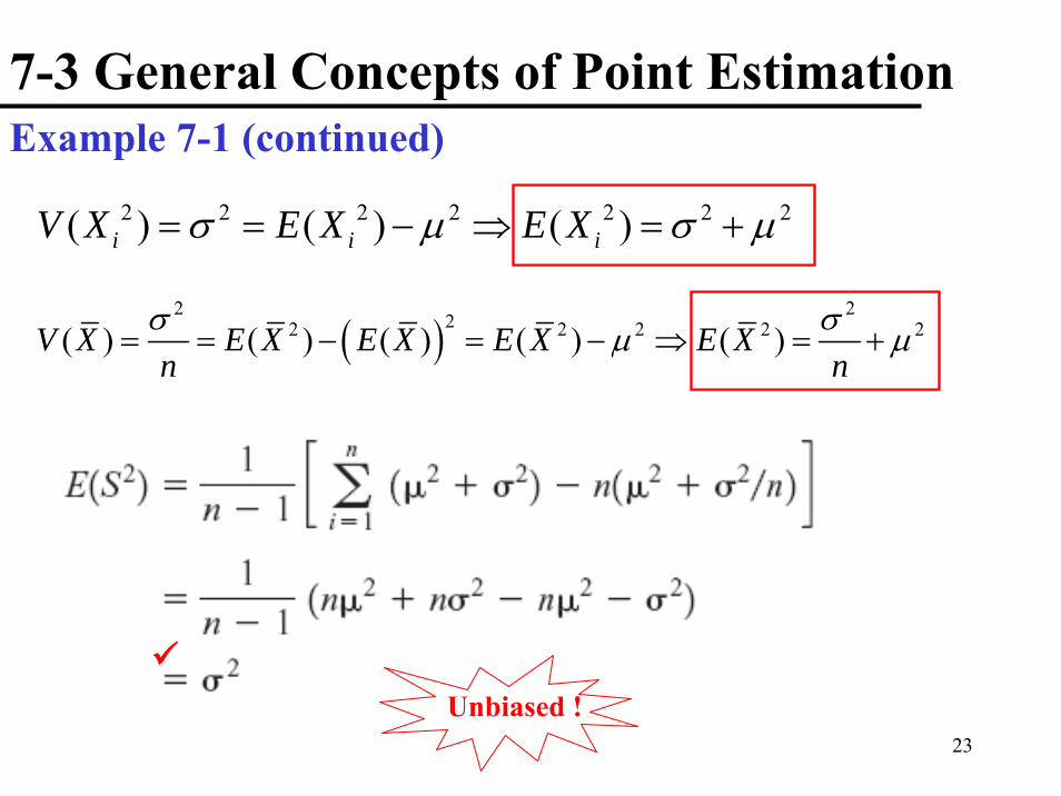
2 2 2 2 2 2 2( ) ( ) ( )i i iV X E X E Xσ μ σ μ= = − ⇒ = +
Example 7-1 (continued)
( )2 2
22 2 2 2 2( ) ( ) ( ) ( ) ( )V X E X E X E X E Xn nσ σμ μ= = − = − ⇒ = +
Unbiased !

24
7-3 General Concepts of Point Estimation
• There is not a unique unbiased estimator.• n=10 data 12.8 9.4 8.7 11.6 13.1 9.8 14.1 8.5 12.1 10.3
• There are several unbiased estimators of µ– Sample mean (11.04)– Sample median (10.95)– The average of the smallest and largest observations in the sample (11.3)– A single observation from the population (12.8)
• Cannot rely on the property of unbiasedness alone to select theestimator.
• Need a method to select among unbiased estimators.
25
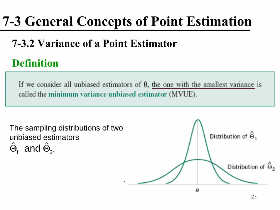
7-3 General Concepts of Point Estimation 7-3.2 Variance of a Point Estimator
Definition
The sampling distributions of two unbiased estimators
.ˆˆ21 ΘΘ and
26
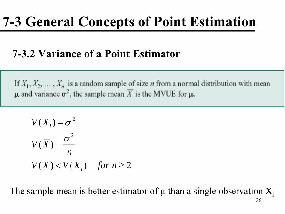
7-3 General Concepts of Point Estimation
7-3.2 Variance of a Point Estimator
2
2
( )
( )
( ) ( ) 2
i
i
V X
V Xn
V X V X for n
σ
σ
=
=
< ≥
The sample mean is better estimator of µ than a single observation Xi
27
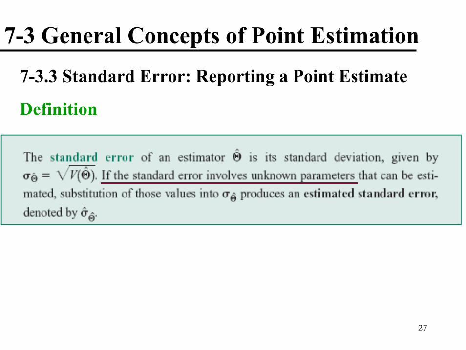
7-3 General Concepts of Point Estimation
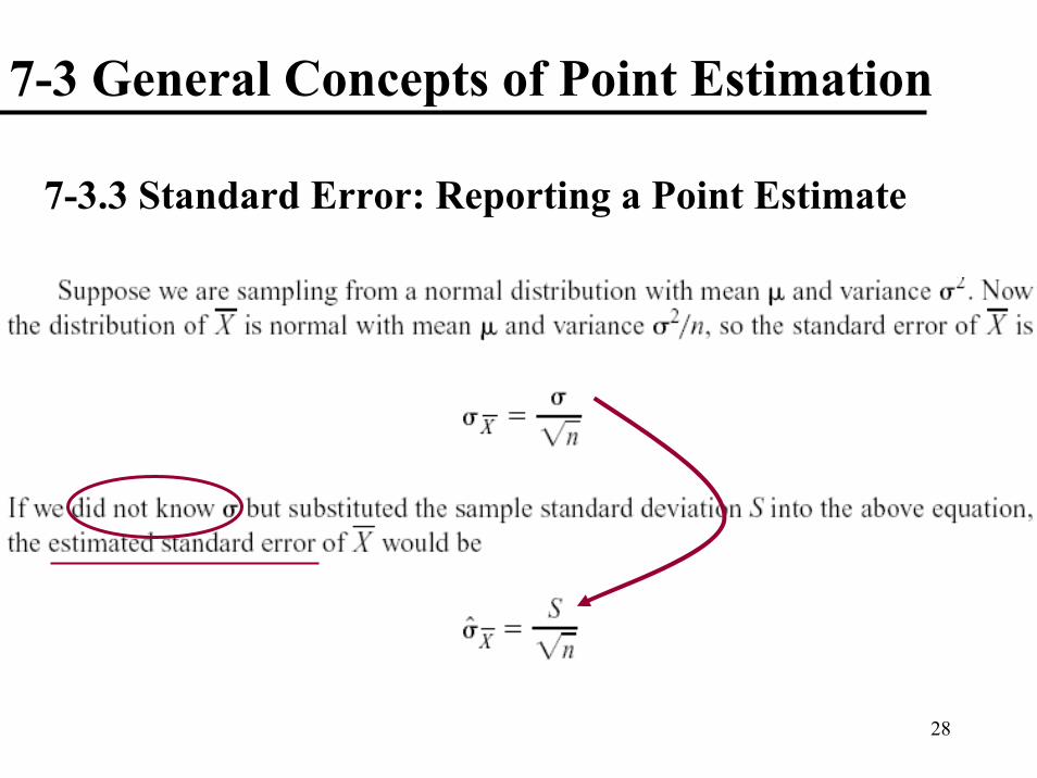
7-3.3 Standard Error: Reporting a Point Estimate
Definition
28
7-3 General Concepts of Point Estimation
7-3.3 Standard Error: Reporting a Point Estimate
29
7-3 General Concepts of Point Estimation
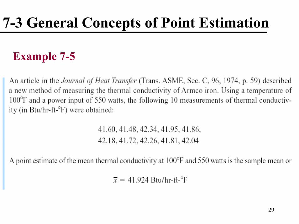
Example 7-5
30
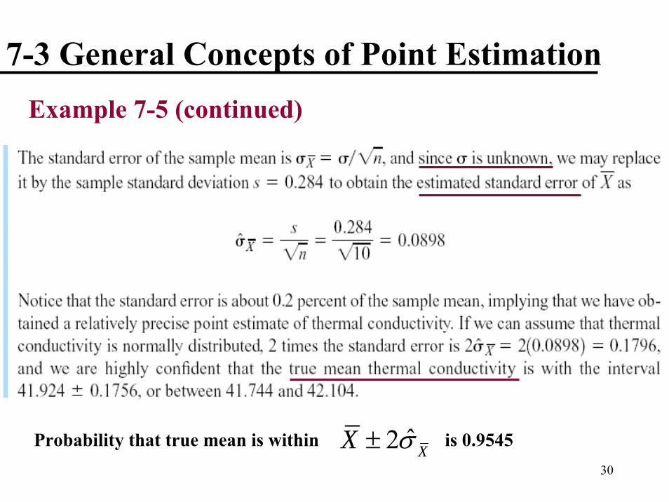
7-3 General Concepts of Point Estimation Example 7-5 (continued)
ˆ2 XX σ±Probability that true mean is within is 0.9545
31
7-3 General Concepts of Point Estimation
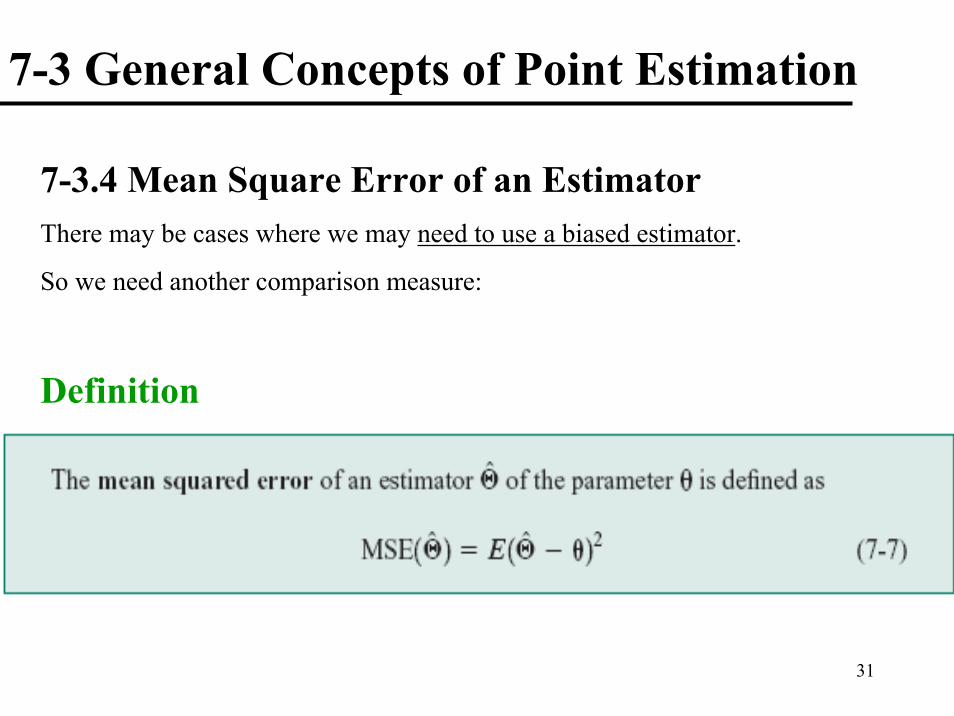
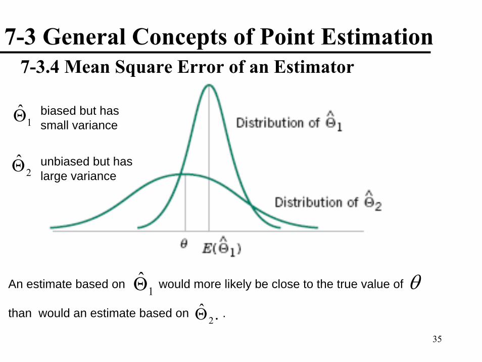
7-3.4 Mean Square Error of an EstimatorThere may be cases where we may need to use a biased estimator.
So we need another comparison measure:
Definition

32
7-3 General Concepts of Point Estimation
Θ̂The MSE of is equal to the variance of the estimator plus the squared bias.
If is an unbiased estimator of θ, MSE of is equal to the variance of
2
2 2
2
ˆ ˆ( ) ( )
ˆ ˆ ˆ( ) ( )
ˆ( ) ( )
MSE E
E E E
V bias
θ
θ
Θ = Θ−
⎡ ⎤ ⎡ ⎤= Θ− Θ + − Θ⎣ ⎦ ⎣ ⎦
= Θ +
Θ̂
Θ̂ ˆ
7-3.4 Mean Square Error of an Estimator
Θ

33
7-3 General Concepts of Point Estimation
2ˆ( ) ( )V biasΘ +2 2
2 2 2 2
2 2 2 2
2 2 2 2
2 2
2
ˆ ˆ ˆ( ) ( )
ˆ ˆ ˆ ˆ ˆ ˆ2 ( ) ( ) 2 ( ) ( )
ˆ ˆ ˆ ˆ ˆ ˆ( ) 2 ( ) ( ) ( ) 2 ( ) ( )ˆ ˆ ˆ ˆ( ) ( ) 2 ( ) ( )ˆ ˆ( ) 2 ( )ˆ( )
E E E
E E E E E
E E E E E E
E E E E
E E
E
θ
θ θ
θ θ
θ θ
θ θ
θ
⎡ ⎤ ⎡ ⎤Θ− Θ + − Θ⎣ ⎦ ⎣ ⎦⎡ ⎤ ⎡ ⎤= Θ − Θ Θ + Θ + − Θ + Θ⎣ ⎦ ⎣ ⎦
= Θ − Θ Θ + Θ + − Θ + Θ
= Θ − Θ + − Θ + Θ
= Θ + − Θ
= Θ−
7-3.4 Mean Square Error of an Estimator
ˆ( )MSE Θ

34
7-3 General Concepts of Point Estimation
7-3.4 Mean Square Error of an Estimator
35
7-3 General Concepts of Point Estimation
1Θ̂
.ˆ2Θ
1Θ̂
7-3.4 Mean Square Error of an Estimator
1Θ̂
An estimate based on would more likely be close to the true value of
than would an estimate based on ..ˆ2Θ
biased but has small variance
2Θ̂ unbiased but has large variance
θ

36
7-3 General Concepts of Point Estimation 7-3.4 Mean Square Error of an Estimator
Exercise: Calculate the MSE of the following estimators.
1
2
ˆ
ˆX
X
Θ =
Θ =

37
7-4 Methods of Point Estimation How can good estimators be obtained?
7-4.1 Method of Moments
38
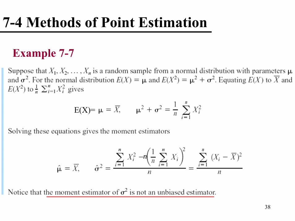
7-4 Methods of Point Estimation
Example 7-7
n
E(X)=
39
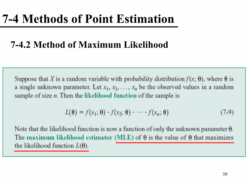
7-4 Methods of Point Estimation
7-4.2 Method of Maximum Likelihood

40
7-4 Methods of Point Estimation
Example 7-9
41
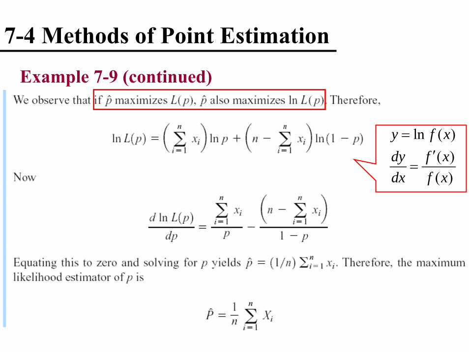
7-4 Methods of Point Estimation
Example 7-9 (continued)
ln ( )( )( )
y f xdy f xdx f x
=′
=

42
7-4 Methods of Point Estimation
Example 7-12
1
( )
( )
m
m
y ax bdy ma ax bdx
−
= +
= +

43
7-4 Methods of Point Estimation
Example 7-12 (continued)
44
7-4 Methods of Point Estimation
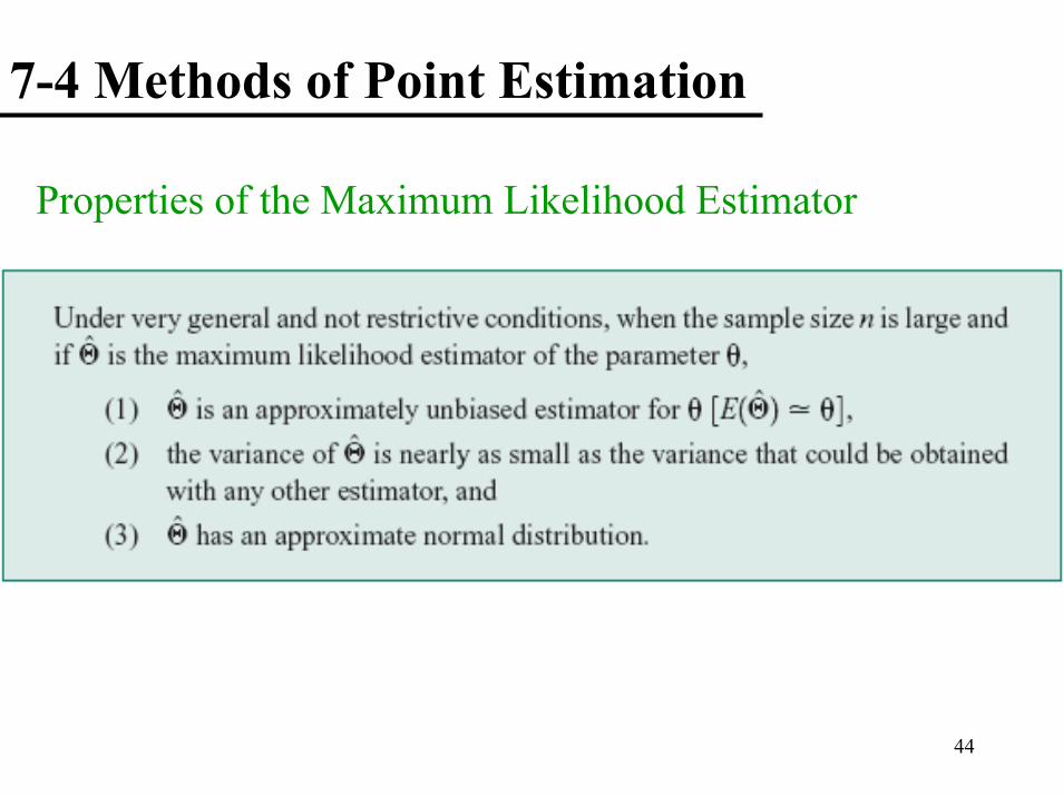
Properties of the Maximum Likelihood Estimator

45
7-4 Methods of Point Estimation
2σ
Properties of the Maximum Likelihood Estimator2
2 2
1
2 2
22 2
1ˆ ( )
1ˆ( )
ˆ( )
n
ii
MLE of is
X Xn
nEn
bias En
σ
σ
σ σ
σσ σ
=
= −
−=
−= − =
∑
bias is negative. MLE for tends to underestimateThe bias approaches zero as n increases.MLE for is an asymptotically unbiased estimator for
2σ
2σ
2σ
46
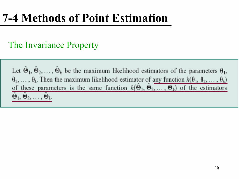
7-4 Methods of Point Estimation
The Invariance Property
47
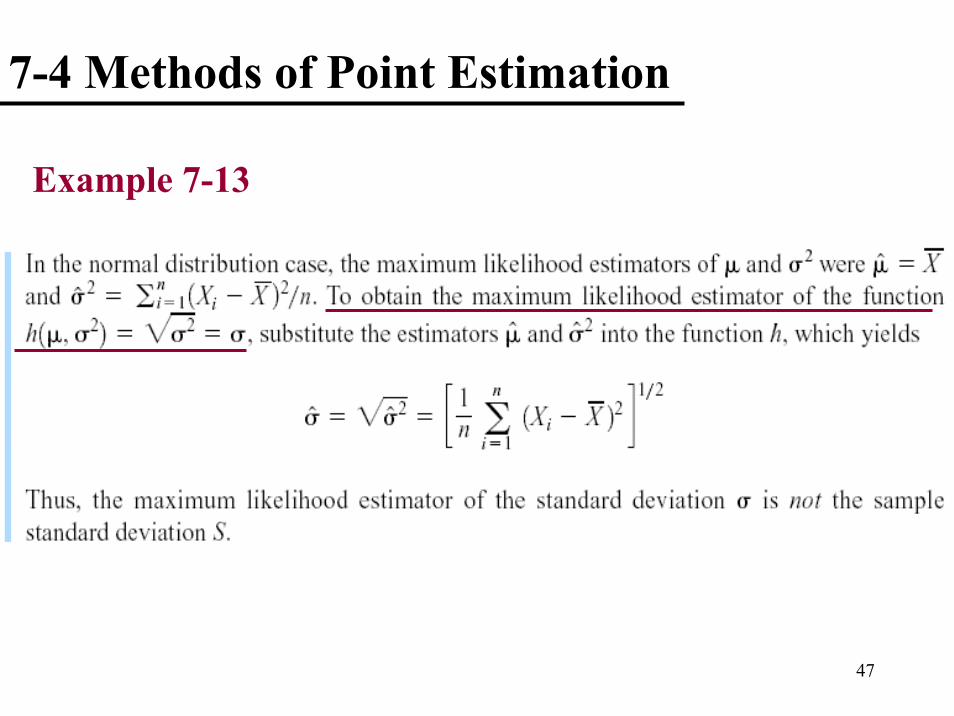
7-4 Methods of Point Estimation
Example 7-13

48
7-4 Methods of Point Estimation
Complications in Using Maximum Likelihood Estimation
• It is not always easy to maximize the likelihood function because the equation(s) obtained from dL(θ)/dθ = 0 may be difficult to solve.
• It may not always be possible to use calculus methods directly to determine the maximum of L(θ).
![[7] Point estimation](https://static.fdocuments.net/doc/165x107/62004a9f43292f22092918e5/7-point-estimation.jpg)