

Ch3graphical Linkage Synthesis
105
Graphical Linkage Synthesis Chapter 3
-
Upload
vishal-pawar -
Category
Documents
-
view
83 -
download
0
description
notes
Transcript of Ch3graphical Linkage Synthesis

Graphical Linkage
SynthesisChapter 3

Synthesis
• Qualitative Synthesis
– The creation of potential solution in
the absence of a well-defined
algorithm that configures or predicts
the solution
• Type Synthesis
– The definition of the proper
mechanism best suitable to the
problem

Synthesis• Quantitative Synthesis
– Generation of one or more solution of
a particular type that you know to be
suitable to the problem, and
importantly, one for which there is a
synthesis algorithm defined
• Dimensional Synthesis
– Is the determination of the
proportions (length) of the links
necessary to accomplish the desired
motions

Function, Path and Motion Generation• Function
– Defined as the correlation of an input
motion with an output motion in a
mechanism
• Path
– Control of a point in the plane such that is
follows some prescribed path
• Motion Generation
– Control of a line in the plane such that is
follows some prescribed set of sequential
positions

Limiting Conditions• Toggle/ Stationary Position

Limiting Conditions• Toggle/Stationary Position

Limiting Conditions• Transmission angle
– Angle between the output link and the
coupler

Dimensional Synthesis• The determination of the proportions
(lengths) of the links necessary to
accomplish the desired motions
• Two-Position synthesis
– Rocker
– Coupler

Example 1• Rocker Output- Two Position with
Angular Displacement (Function)
– Design a four bar Grashof crank-rocker
speed motor input to give 45° of rocker
motion with equal time forward and back,
from a constant speed motor input.

Example 1• 1. Draw the output
link O4B in both
extreme positions,
B1 and B2 in any
convenient location,
such that the
desired angle of
motion θ4 is
subtended.

• 2. Draw the chord
B1B2 and extended
it in either direction.

• 3. Select a
convenient point O2
on the line B1B2
extended.

• 4. Bisect line
segment B1B2, draw
a circle of that
radius about O2.

• 5. Label the two
intersection of the
circle and B1B2
extended, A1 and
A2.

• 6. Measure the
length of the coupler
as A1 to B1 or A2 to
B2.

• 8. Find the Grashof
condition. If non-
Grashof, redo steps
3 to 8 with O2 further
from O4.

• 9. Make model of
the linkage and
check its function
and transmission
angles.

Example 1
• 10. You can input
the file F03-04.4br

Example 2• Rocker Output- Two Position with
Complex Displacement (Motion)
– Design a fourbar linkage to move link CD
from C1D1 to C2D2.

Example 2• 1. Draw the link CD
in its two desired
positions, C1D1 and
C2D2 in plane as
shown.
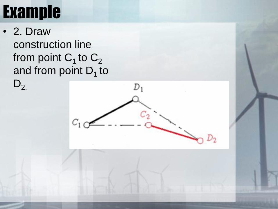
Example • 2. Draw
construction line
from point C1 to C2
and from point D1 to
D2.

Example • 3. Bisect line C1C2
and line D1D2 and
extend their
perpendicular
bisectors to
intersect at O4.
Their intersection is
the rotopole.

Example • 4. Select a
convenient radius
and draw an arc
about the rotopole
to intersect both
lines O4C1 and
O4C2. Label the
intersection B1 and
B2.

Example • 5. Do steps 2 to 8 of
example 1 to
complete the
linkage.
• 6. Make a model of
the linkage and
articulate it to check
its function and its
transmission
angles.
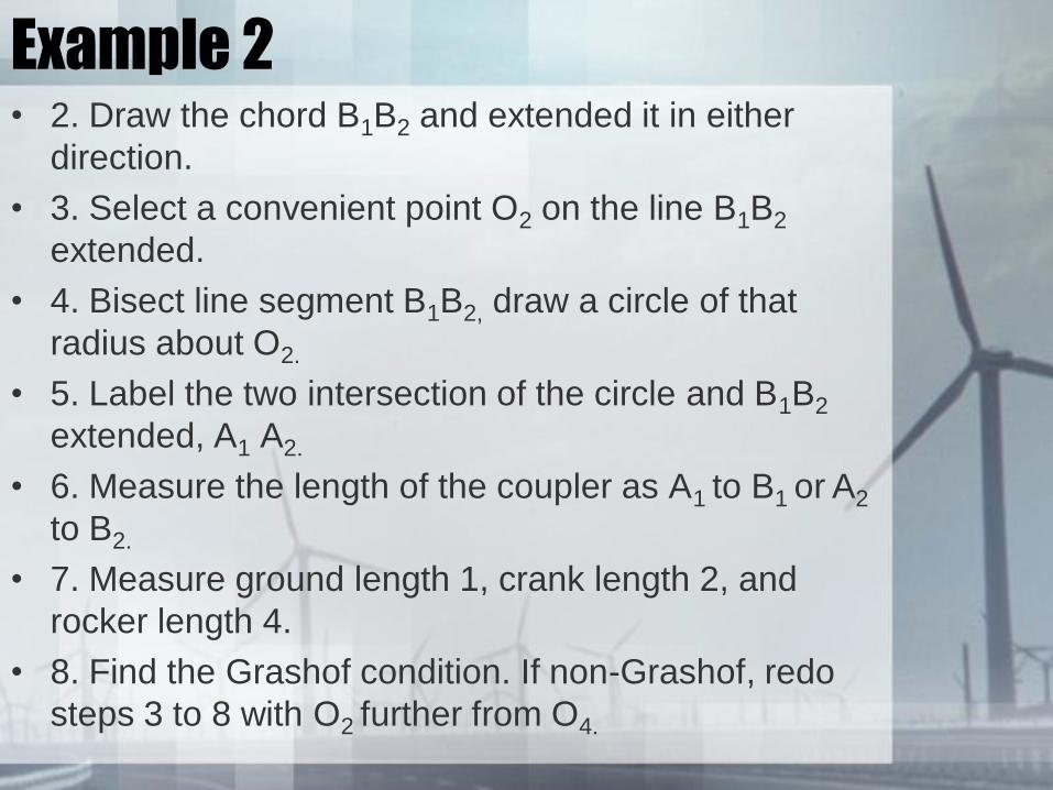
Example 2 • 2. Draw the chord B1B2 and extended it in either
direction.
• 3. Select a convenient point O2 on the line B1B2
extended.
• 4. Bisect line segment B1B2, draw a circle of that
radius about O2.
• 5. Label the two intersection of the circle and B1B2
extended, A1 A2.
• 6. Measure the length of the coupler as A1 to B1 or A2
to B2.
• 7. Measure ground length 1, crank length 2, and
rocker length 4.
• 8. Find the Grashof condition. If non-Grashof, redo
steps 3 to 8 with O2 further from O4.

Example 3• Coupler Output- Two Position with
Complex Displacement (Motion)
– Design a fourbar linkage to move link CD
from C1D1 to C2D2 (with moving pivots at
C and D).
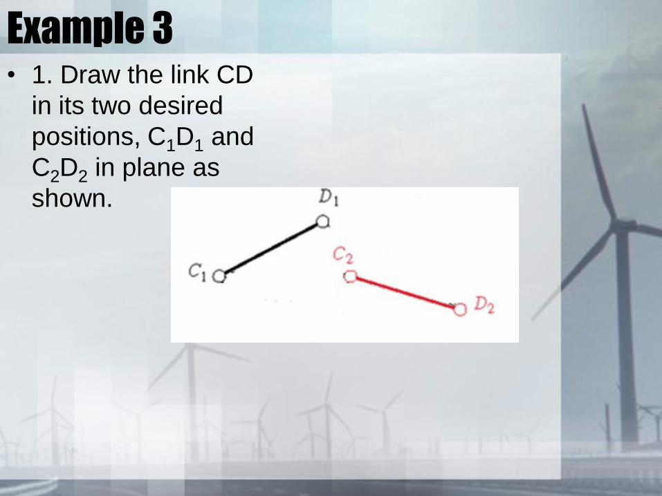
Example 3• 1. Draw the link CD
in its two desired
positions, C1D1 and
C2D2 in plane as
shown.

Example • 2. Draw
construction line
from point C1 to C2
and from point D1 to
D2.

Example • 3. Bisect line C1C2
and line D1D2 and
extend their
perpendicular
bisectors in
convenient
directions.The
rotopole will not be
used in this solution.

Example • 4. Select any
convenient point on
each bisector as the
fixed pivots O2 and
O4 , respectively.

Example • 5. Connect O2 with C1
and call it link 2.
Connect O4 with D1 and
call it link 4.
• 6. Line C1D1 is link 3.
Line O2O4 is link 1.
• 7. Check the Grashof
condition, and repeat
steps 4 to 7 if
unsatisfied. Note that
any Grashof condition
is potentially acceptable
in this case.
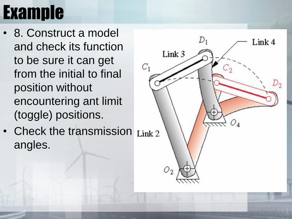
Example • 8. Construct a model
and check its function
to be sure it can get
from the initial to final
position without
encountering ant limit
(toggle) positions.
• Check the transmission
angles.

Example • Review Example 3-4
– Design a dyad to control
and limits the extremes
of motion of the linkages
in the previous example
to its two design
positions

Three-Position Synthesis• Example 1 – Coupler
Output – 3 position with
Complex Displacement
– Design a fourbar linkage to
move the link CD shown
from position C1D1 to C2D2
and then to position C3D3.
Moving pivots are C and D.
Find the fixed pivot locations.

Three-Position Synthesis• 1. Draw link CD in its three position
C1D1, C2D2 , C3D3 in the plane as shown.

Three-Position Synthesis• 2. Draw construction lines from point C1 to C2
and from C2 to C3.

Three-Position Synthesis• 3. Bisect line C1C2 and line C2C3 and extend
their perpendicular bisector until they
intersect. Label their intersection O2.

Three-Position Synthesis• 4. Repeat steps 2 and 3 for lines D1D2 and
D2D3. Label the intersection O4.

Three-Position Synthesis• 5. Connect O2 with C1 and call link 2. Connect
O4 with D1 and call link 4.
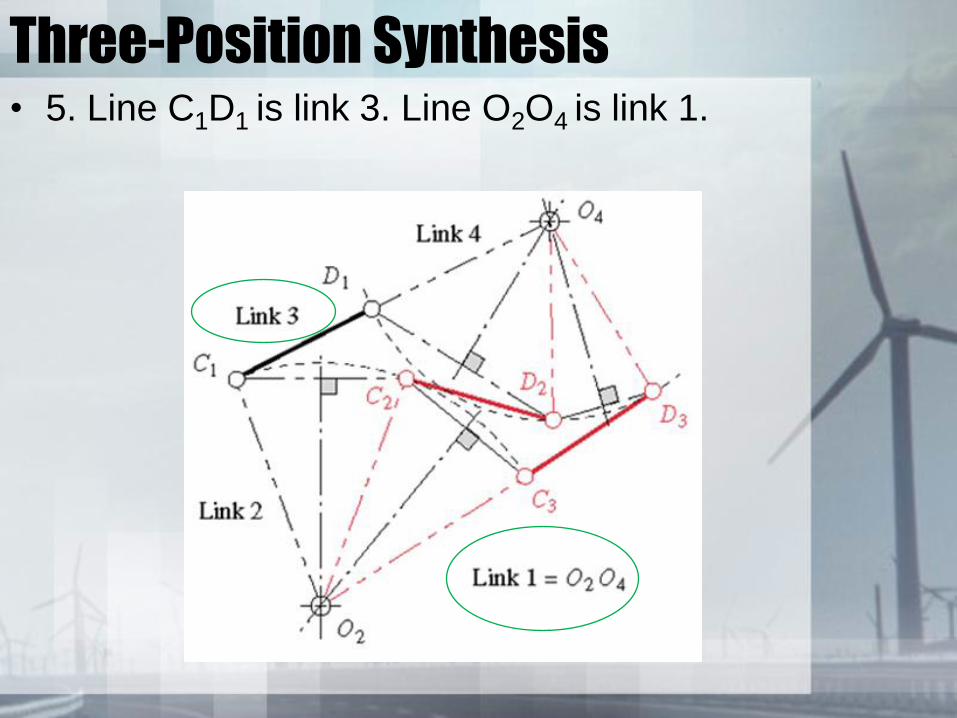
Three-Position Synthesis• 5. Line C1D1 is link 3. Line O2O4 is link 1.

Three-Position Synthesis• 7. Check the Grashof
condition. Note that any
Grashof condition is
potentially acceptable in this
case.
• 8.Construct a model and
check its function to be sure it
can get from initial to final
position without encountering
any limits positions.
• 9.Construct a driver dyad
using an extension of link 3
attach the dyad.

Three-Position Synthesis – Example 2• Example 2 – Coupler
Output – 3 position with
Complex Displacement –
Alternate Attachment Points
for Moving Pivots
– Design a fourbar linkage to
move the link CD shown
from position C1D1 to C2D2
and then to position C3D3.
Use different moving pivot
than CD. Find the fixed pivot
locations.

Three-Position Synthesis – Example 2• 1. Draw link CD in its three
position C1D1, C2D2 , C3D3 in the
plane as shown.
• 2. Define new attachment points
E1 and F1 that have a fixed
relationship between C1D1 and
E1F1 within the link. Now use
E1F1 to define the three position
of the link.
• 3. Draw construction lines from
point E1 to E2 and from E2 to E3.

Example 2• 4. Bisect line E1E2 and line E2E3
and extend their perpendicular
bisector until they intersect.
Label their intersection O2.
• 5. Repeat steps 2 and 3 for lines
F1F2 and F2F3. Label the
intersection O4.
• 6. Connect O2 with E1 and call
link 2. Connect O4 with F1 and
call link 4.
• 7. Line E1F1 is link 3. Line O2O4 is
link 1

Example 2• 8. Check the Grashof
condition. Note that any
Grashof condition is
potentially acceptable in this
case.
• 9.Construct a model and
check its function to be sure it
can get from initial to final
position without encountering
any limits positions. If not,
change locations of point E
and F and repeat steps 3 to 9.
Three-Position Synthesis – Example 3• Example 3 – Three –Position Synthesis
with Specified Fixed Pivots - Inverting
the 3-position problem
– Invert a fourbar linkage which move the
link CD shown from position C1D1 to C2D2
and then to position C3D3. Use specified
fixed pivots O2 and O4.

Example 3• 1. Draw link CD in its three position C1D1,
C2D2 , C3D3 in the plane as shown.
• 2. Draw the ground link O2O4 in its desired
position in the plane with respect to the first
coupler position C1D1

Example 3• 3. Draw construction arc from point C2 to O2
and from D2 to O2 whose radii define the side
of triangle C2O2D2 This define the
relationship of the fixed pivot O2 to the
coupler line CD in the second coupler
position.
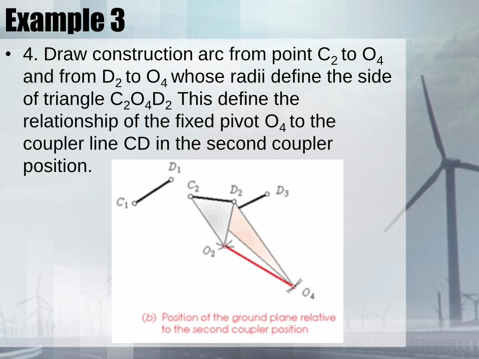
Example 3• 4. Draw construction arc from point C2 to O4
and from D2 to O4 whose radii define the side
of triangle C2O4D2 This define the
relationship of the fixed pivot O4 to the
coupler line CD in the second coupler
position.

Example 3• 5. Now transfer this relationship back
to the first coupler position C1D1 so
that the ground plane position O2’O4’
bears the same relationship to C1D1
as O2O4 bore to the second coupler
position C2D2. In effect, you are
sliding C2 along the dotted line C2C1
and D2 along the dotted D2D1. By
doing this, we have pretended that
ground plane moved from O2O4 to
O2’O4’ instead of the coupler moving
from C1D1 to C2D2. We have inverted
the problem.

Example 3• 6. Repeat the process for the third coupler
position as shown in the figure and transfer
the third relative ground link position to the
first, or reference, position.

Example 3• 7. The three inverted position of the ground
plane that correspond to the three desired
coupler positions are labeled O2O4,O2’O4’ ,
and O2’’O4’’ and have also been renamed
E1F1, E2F2 and E3F3 as shown in the figure

Three-Position Synthesis – Example 4• Example 4 – Finding the Moving Pivots
for Three Positions and Specified Fixed
Pivots
– Design a fourbar linkage to move the link
CD shown from position C1D1 to C2D2 and
then to position C3D3. Use specified fixed
pivots O2 and O4. Find the required moving
pivot location on the coupler by inversion.

Example 4• 1. Start with inverted three positions plane as
shown in the figures. Lines E1F1, E2F2 and
E3F3 define the three positions of the inverted
link to be moved.

Example 4• 2. Draw construction lines from point E1 to E2
and from point E2 to E3.

Example 4• 3. Bisect line E1E2 and line E2E3 extend the
perpendicular bisector until they intersect.
Label the intersection G.

Example 4• 4. Repeat steps 2 and 3 for lines F1F2 and
line F2F3. Label the intersection H.

Example 4• 5. Connect G with E1 and call it link 2.
Connect H with F1 and call it link 4.

Example 4• 6. In this inverted linkage, line E1F1 is the
coupler, link 3. Line GH is the “ground” link1.

Example 4• 7. We must now reinvert the linkage to return to
the original arrangement. Line E1F1 is really the
ground O2O4 and GH is really the coupler. The
figure shows the reinversion of the linkage in
which points G and H are now the moving pivots
on the coupler and E1F1 has resumed its real
identity as ground link O2O4.

Example 4• 8. The figure reintroduces the original line C1D1
in its correct relationship to line O2O4 at the initial
position as shown in the original example 3. This
form the required coupler plane and defines a
minimal shape of link 3.

Example 4• 9. The angular motions required to
reach the second and third position
of line CD shown in the figure are
the same as those defined in figure
b for the linkage inversion. The
angle F1HF2 in the figure b is the
same as the angle H1O4H2 in the
figure and F2HF3 is the same as
angle H2O4H3. The angular
excursions of link 2 retain the same
between figure b and e as well. The
angular motions of links 2 and 4 are
the same for both inversion as the
link excursions are relative to one
another.

Example 4

Example 4• 10. Check the Grashof condition. Note that any
Grashof condition is potentially acceptable in this
case provided that the linkage has mobility
among all three position. This solution is a non-
Grashof linkage.
• 11. Construct a model and check its function to
be sure it can get from initial to final position
without encountering any limit (toggle) positions.
In this case link 3 and 4 reach a toggle position
between points H1 and H2. This means that this
linkage cannot be driven from link 2 as it will
hang up at that toggle position. It must driven
from link 4.
Instructional Videos• Professor Robert Norton’s Instructional
Videos are included on the book’s
DVD. Please watch the following
videos;
– Quick-Return Mechanisms
– Coupler Curves
– Cognates
– Parallel Motion
– Dwell Mechanisms

Quick – Return Mechanism• Fourbar Quick-Return
– Time ratio (TR) defines the degree of quick-return
of the linkage.
– Works well for time ratios down to about 1.5
RT 360
180180
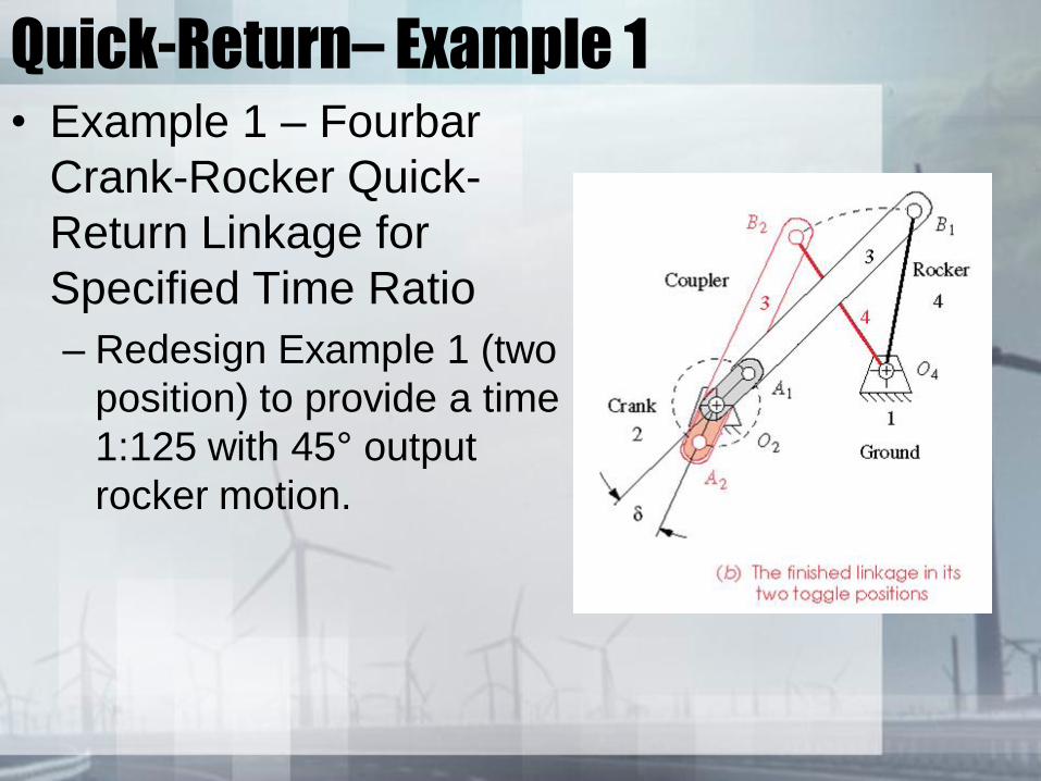
Quick-Return– Example 1• Example 1 – Fourbar
Crank-Rocker Quick-
Return Linkage for
Specified Time Ratio
– Redesign Example 1 (two
position) to provide a time
1:125 with 45° output
rocker motion.

Example 1• 1. Draw the output link O4B in both extreme
position, in any convenient location, such that
the desired angle of motion, θ4 , is
subtended.

Example 1• 2. Calculate α, β, δ using the
equations. In this example
α=160°, β=200°, δ=20°.
• 3. Draw a construction line
through point B1 at any
convenient angle.
• 4. Draw a construction line
through point B2 at an angle δ
from the first line.
• 5. Label the intersection of the
two construction line O2.
• 6. The line O2O4 define ground.

Example 1• 7. Calculate the length of crank
and coupler by measuring O2B1
and O2B2 and solve
simultaneously;
coupler + crank=O2B1
coupler - crank=O2B2
or you can construct the crank
length by swinging an arc centered
at O2 from B1 to cut line O2B2
extended. Label that intersection
B1’. The line B2B1’ is twice the
crank length. Bisect this line
segment to measure crank length
O2A1.

Example 1• 8. Calculate the Grashof condition.
If non-Grashof, repeat steps 3 to 8
with O2 further O4.
• 9. Make a model of the linkage
and articulate it to check its
function.
• 10. Check the transmission angle.

Quick-Return– Example 2• Example 2 – Sixbar
Drag Link Quick-
Return Linkage for
Specified Time Ratio
– Provide a time ratio of
1:1.4 with 90 degree
rocker motion
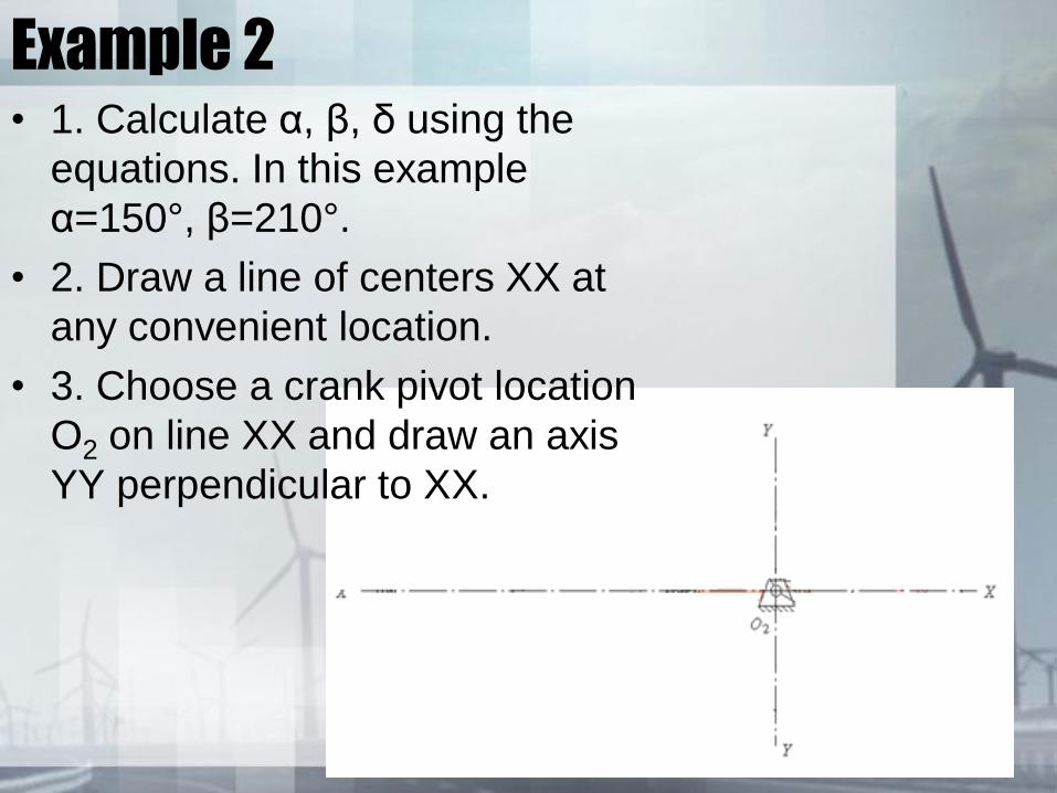
Example 2• 1. Calculate α, β, δ using the
equations. In this example
α=150°, β=210°.
• 2. Draw a line of centers XX at
any convenient location.
• 3. Choose a crank pivot location
O2 on line XX and draw an axis
YY perpendicular to XX.

Example 2• 4. Draw a line of convenient
radius O2A about center O2
• 5. Lay out angle α with vertex at
O2, symmetrical about quadrant
one
• 6. Label points A1 and A2 at the
intersection of the lines
subtending angle α and the
circle of radius O2A.

Example 2• 7. Set the compass to a
convenient radius AC long
enough to cut XX in two places
on either side of O2 when
swung from A1 and A2. Label
the intersection C1 and C2.
• 8. The line O2A1 id the driver
crank, link 2, and line A1C1 is
the coupler, link 3.
• 9. The distance C1C2 is twice
the driven (dragged) crank
length. Bisect it to locate the
fixed pivot O4.

Example 2• 10. The line O2O4 now defines
the ground link. Link O4C1 is
the driven crank, link 4.
• 11. Calculate the Grashof
condition. If Non-Grashof,
repeat steps 7-11 with a shorter
radius in step 7.

Example 2• 12. invert the method of example 1 (two
positions) to create the output dyad using XX
as the chord and O4C1 as the driving crank.
The point B1 and B2 will lie on line XX and be
spaced apart a distance 2O4C1. The pivot O6
will lie on the perpendicular bisector of B1B2,
at a distance from line XX which subtends the
specified output rocker angle.
• 13. Check the transmission angle.

Cognates• Roberts-Chebyschev
– Three different planar fourbar linkages will
trace identical coupler curves.
• Cayley Diagram: Construction lines parallel to
all sides of the links
• Roberts Diagram: Three fourbars linkage
cognates which shares the same coupler curve

Cognates- Parallel Motion

Cognates- Parallel Motion

Cognates- Geared Fivebar Cognates• Chebyschev discovered that any
fourbar coupler curve can be duplicated
with a geared fivebar mechanism
whose gear ratio is plus one, meaning
that the gears turn with the same speed
and direction.

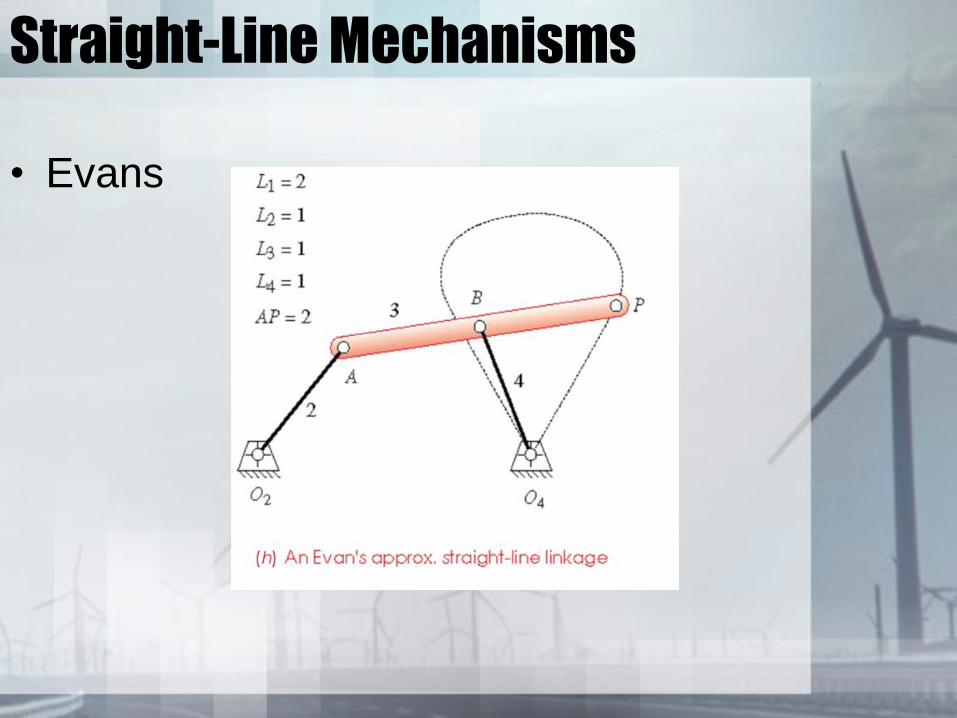
Straight-Line Mechanisms• Watt’s

Dwell Mechanisms• Is defined as zero output for some
nonzero input motion
– Single-Dwell: Design a sixbar linkage for
90° rocker motion over 300 crank degree
with dwell for the remaining 60°

Dwell Mechanisms-Example 1• 1. Search the H&N atlas for a
fourbar linkage with a coupler
curve having an approximate
(pseudo) circle arc portion
which occupies 60° of crank
motion (12 dashes). The
chosen fourlink is shown in the
figure.
• 2. Lay out this linkage to scale
including the coupler curve and
find the approximate center of
the chosen coupler curve using
graphical techniques.

Example 1• 2. To do so, draw the chord of the arc and
construct its perpendicular bisector. The center
lie on this bisector. Find it by striking arcs with
your compass point on the bisector, while
adjusting the radius to get best fit to the coupler.
Label the arc center D.

Example 1• 3. Your compass should now be
set to the approximate radius of
the coupler arc. This will be the
length of link 5 which is to be
attached at the coupler point P.
• 4. Trace the coupler curve with
the compass point, while keeping
the compass pencil lead on the
perpendicular bisector, and find
the extreme location along the
bisector that the compass lead
will reach. Label this point E.
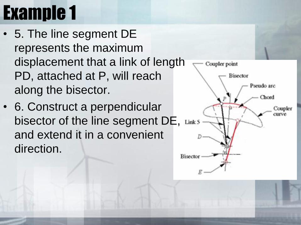
Example 1• 5. The line segment DE
represents the maximum
displacement that a link of length
PD, attached at P, will reach
along the bisector.
• 6. Construct a perpendicular
bisector of the line segment DE,
and extend it in a convenient
direction.

Example 1• 7. Locate fixed pivot O6 on the
bisector of DE such line O6D and
O6E subtend the desired output
angle, 90°.
• 8. Draw link 6 from D (or E)
through O6 and extend to any
convenient length. This is the
output link which will dwell for
specified portion of the crank
cycle.
• Check the transmission angles.

Example 1– Single-Dwell: Design a sixbar linkage for
90° rocker motion over 300 crank degree
with dwell for the remaining 60°

Dwell Mechanisms-Example 2– Double-Dwell: Design a sixbar linkage for
80° rocker motion over 20 crank degree
with dwell for the remaining 160°, return
motion over 140° and second dwell for 40°.

Example 2• 1. Search the H&N atlas for a
linkage with a coupler curve
having two approximate straight-
line portions. One should occupy
160° of crank motion (32 dashes),
and the second 40° of crank
motion (8 dashes). This is a
wedge-shaped curve.
• 2. Lay out this linkage to scale
including the coupler curve and
find the intersection of two tangent
lines colinear with the straight
segment. Label this point O6.

Example 2• 3. Design link 6 to lie along
these straight tangent, pivoted
at O6. Provide a slot in link 6 to
accommodate slider block 5.
• 4. Connect slider block 5 to the
coupler point P on link 3 with a
pin joint. The finish sixbar is
shown in the next figure.
• Check transmission angle.

Example 2– Double-Dwell