Ch.14: Query OptimizationCh.14: Query Optimization

Introduction Introduction Catalog Information for Cost EstimationCatalog Information for Cost Estimation Estimation of StatisticsEstimation of Statistics Transformation of Relational ExpressionsTransformation of Relational Expressions Dynamic Programming for Choosing Dynamic Programming for Choosing

Evaluation PlansEvaluation Plans

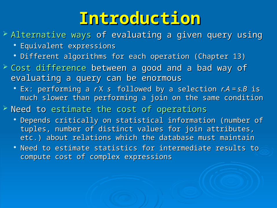
IntroductionIntroduction Alternative waysAlternative ways of evaluating a given query using of evaluating a given query using

Equivalent expressionsEquivalent expressions Different algorithms for each operation (Chapter 13)Different algorithms for each operation (Chapter 13)

Cost differenceCost difference between a good and a bad way of evaluating a between a good and a bad way of evaluating a query can be enormousquery can be enormous ExEx: : performing a performing a r r X X s s followed by a selection followed by a selection r.A = s.Br.A = s.B is much slower is much slower

than performing a join on the same conditionthan performing a join on the same condition

Need to Need to estimate the cost of operationsestimate the cost of operations Depends critically on statistical information (number of tuples, number of Depends critically on statistical information (number of tuples, number of

distinct values for join attributes, etc.) about relations which the database distinct values for join attributes, etc.) about relations which the database must maintainmust maintain

Need to estimate statistics for intermediate results to compute cost of Need to estimate statistics for intermediate results to compute cost of complex expressionscomplex expressions

ExampleExampleRelations generated by two equivalent expressions have the same set of attributes Relations generated by two equivalent expressions have the same set of attributes and contain the same set of tuples, although their attributes may be ordered and contain the same set of tuples, although their attributes may be ordered differently.differently.

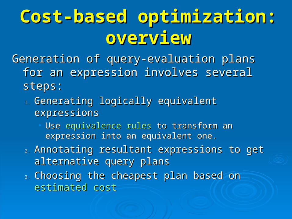
Cost-based optimization: Cost-based optimization: overviewoverview

Generation of query-evaluation plans for an Generation of query-evaluation plans for an expression involves several steps:expression involves several steps:1.1. Generating logically equivalent expressionsGenerating logically equivalent expressions

• Use Use equivalence rulesequivalence rules to transform an expression to transform an expression into an equivalent one.into an equivalent one.

2.2. Annotating resultant expressions to get Annotating resultant expressions to get alternative query plansalternative query plans

3.3. Choosing the cheapest plan based on Choosing the cheapest plan based on estimated estimated costcost

Detailed plan of chapterDetailed plan of chapter

Statistical information for cost estimationStatistical information for cost estimation Equivalence rulesEquivalence rules Cost-based optimization algorithmCost-based optimization algorithm Optimizing nested subqueriesOptimizing nested subqueries Materialized views and view maintenanceMaterialized views and view maintenance

Statistical Information for Statistical Information for Cost EstimationCost Estimation

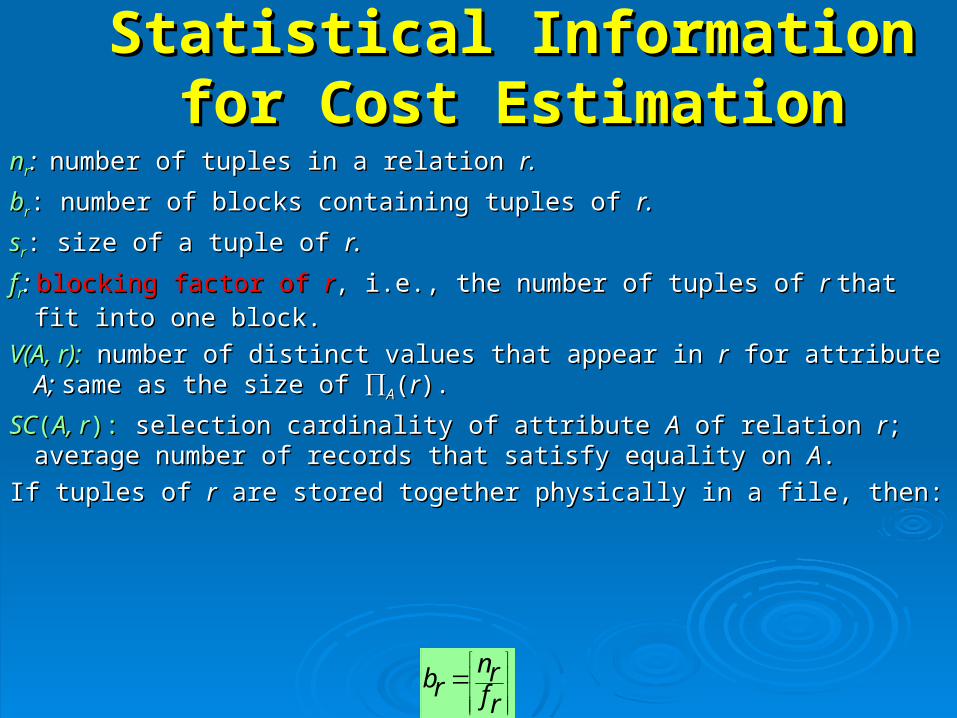
nnrr: : number of tuples in a relation number of tuples in a relation r.r.

bbrr: number of blocks containing tuples of : number of blocks containing tuples of r.r.

ssrr: size of a tuple of : size of a tuple of r.r.

ffrr: : blocking factor of blocking factor of rr, i.e., the number of tuples of , i.e., the number of tuples of r r that fit into one block.that fit into one block.

V(A, r):V(A, r): number of distinct values that appear in number of distinct values that appear in rr for attribute for attribute A; A; same as same as the size of the size of AA((rr).).

SCSC((A, rA, r):): selection cardinality of attribute selection cardinality of attribute AA of relation of relation rr; average number ; average number of records that satisfy equality on of records that satisfy equality on AA..

If tuples of If tuples of rr are stored together physically in a file, then: are stored together physically in a file, then:

rfrn

rb

Catalog Information about Catalog Information about IndicesIndices

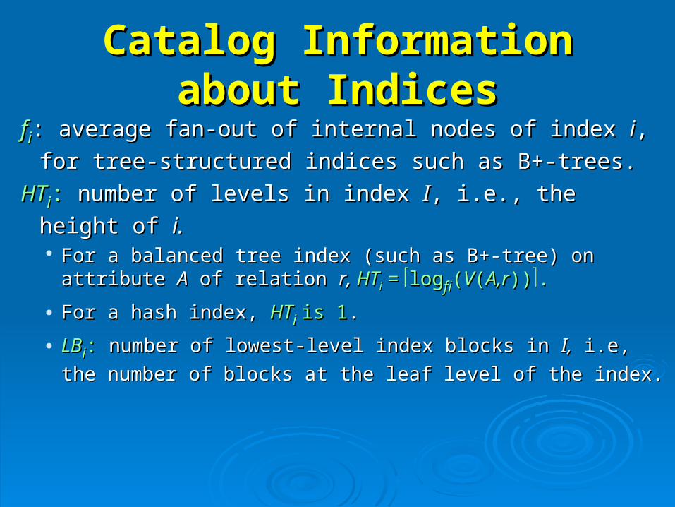
ffii: average fan-out of internal nodes of index : average fan-out of internal nodes of index ii, for tree-, for tree-

structured indices such as B+-trees.structured indices such as B+-trees.

HTHTii:: number of levels in index number of levels in index II, i.e., the height of , i.e., the height of i.i. For a balanced tree index (such as B+-tree) on attribute For a balanced tree index (such as B+-tree) on attribute AA

of relation of relation r, r, HTHTii = = loglogfifi((VV((A,rA,r))))..

For a hash index, For a hash index, HTHTii is 1is 1..

LBLBii:: number of lowest-level index blocks in number of lowest-level index blocks in I,I, i.e, the i.e, the

number of blocks at the leaf level of the index.number of blocks at the leaf level of the index.

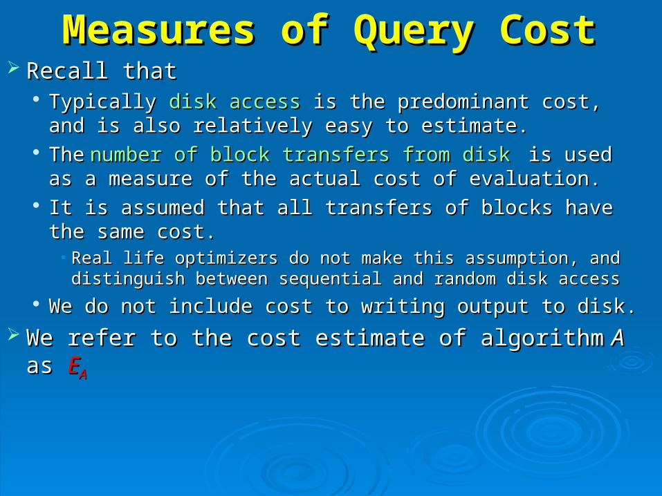
Measures of Query CostMeasures of Query Cost Recall that Recall that

Typically Typically disk accessdisk access is the predominant cost, and is is the predominant cost, and is also relatively easy to estimate. also relatively easy to estimate.

TheThe number of block transfers from disknumber of block transfers from disk is used as a is used as a measure of the actual cost of evaluation.measure of the actual cost of evaluation.

It is assumed that all transfers of blocks have the same It is assumed that all transfers of blocks have the same cost.cost.• Real life optimizers do not make this assumption, and Real life optimizers do not make this assumption, and

distinguish between sequential and random disk accessdistinguish between sequential and random disk access We do not include cost to writing output to disk.We do not include cost to writing output to disk.

We refer to the cost estimate of algorithmWe refer to the cost estimate of algorithm A A as as EEAA

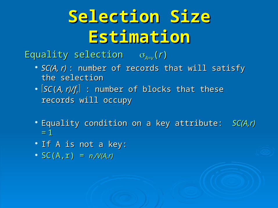
Selection Size EstimationSelection Size Estimation

Equality selection Equality selection A=vA=v((rr)) SC(A, r) SC(A, r) : number of records that will satisfy the : number of records that will satisfy the

selectionselection SCSC((A, r)/fA, r)/frr : number of blocks that these records will : number of blocks that these records will

occupyoccupy

Equality condition on a key attribute: Equality condition on a key attribute: SC(A,r) = SC(A,r) = 11 If A is not a key:If A is not a key: SC(A,r) = SC(A,r) = nnrr/V(A,r)/V(A,r)

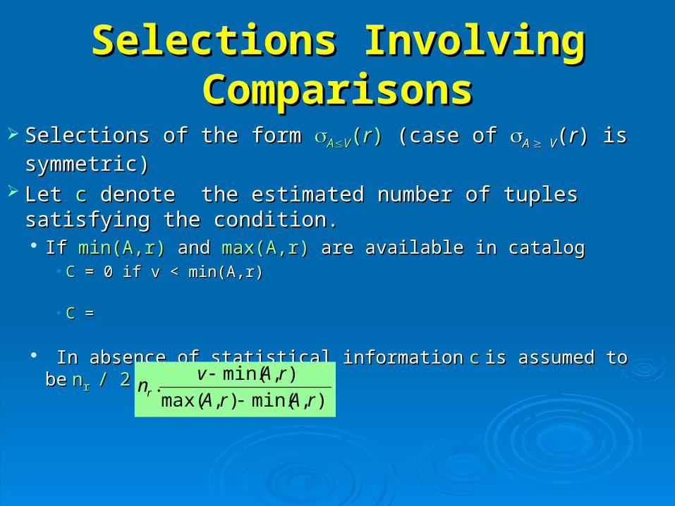
Selections Involving Selections Involving ComparisonsComparisons

Selections of the form Selections of the form AAVV((rr)) (case of (case of A A VV((rr) is ) is

symmetric)symmetric) Let Let cc denote the estimated number of tuples satisfying the denote the estimated number of tuples satisfying the

condition. condition. If If min(A,r)min(A,r) and and max(A,r)max(A,r) are available in catalog are available in catalog

• CC = 0 if v < min(A,r) = 0 if v < min(A,r)

• CC = =

In absence of statistical informationIn absence of statistical information cc is assumed to beis assumed to be nnr r / 2./ 2.),min(),max(

),min(.

rArA

rAvnr

Implementation of Complex Implementation of Complex SelectionsSelections

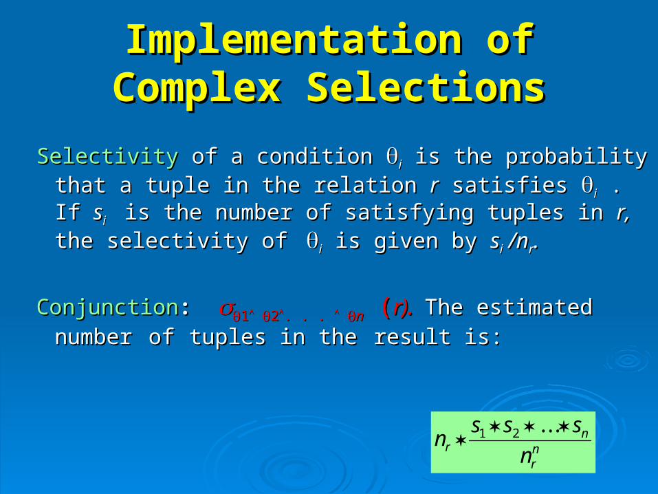
SelectivitySelectivity of a condition of a condition ii is the probability that a tuple in is the probability that a tuple in the relation the relation rr satisfies satisfies ii . If . If ssii is the number of satisfying is the number of satisfying tuples in tuples in r, r, the selectivity of the selectivity of ii is given by is given by ssii /n /nrr..

ConjunctionConjunction: : 11 22. . . . . . nn ( (r).r). The estimated numberThe estimated number ofof tuples in thetuples in the result is:result is:

nr

nr n

sssn

. . . 21

Implementation of Complex Implementation of Complex Selections (cont.)Selections (cont.)

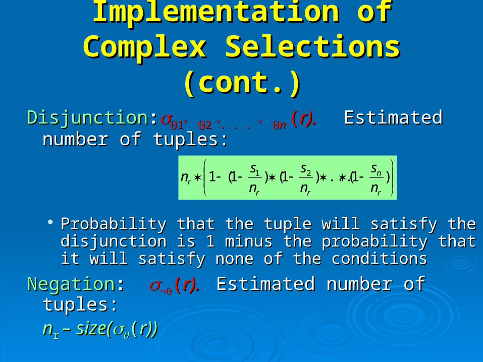
DisjunctionDisjunction::11 22 . . . . . . n n ((r).r). Estimated number Estimated number of tuples:of tuples:

Probability that the tuple will satisfy the Probability that the tuple will satisfy the disjunction is 1 minus the probability that it will disjunction is 1 minus the probability that it will satisfy none of the conditionssatisfy none of the conditions

NegationNegation: : ((r).r). Estimated number of tuples: Estimated number of tuples:nnrr –– size(size(((r))r))

)1(...)1()1(1 21

r

n

rrr n

s

n

s

n

sn

Statistical Information for Statistical Information for ExamplesExamples

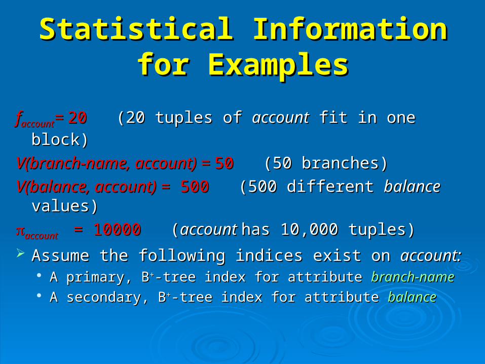
ffaccountaccount= = 2020 (20 tuples of (20 tuples of accountaccount fit in one block) fit in one block)

V(branch-name, account) = V(branch-name, account) = 5050 (50 branches) (50 branches)

V(balance, account) V(balance, account) = 500= 500 (500 different (500 different balancebalance values)values)

accountaccount = 10000 = 10000 ( (account account has 10,000 tuples)has 10,000 tuples)

Assume the following indices exist on Assume the following indices exist on account:account: A primary, BA primary, B++-tree index for attribute -tree index for attribute branch-namebranch-name A secondary, BA secondary, B++-tree index for attribute -tree index for attribute balancebalance

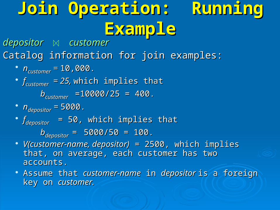
Join Operation: Running Join Operation: Running ExampleExample

depositor depositor customercustomerCatalog information for join examples:Catalog information for join examples:

nncustomercustomer = = 10,000.10,000. ffcustomercustomer = 25, = 25, which implies that which implies that

bbcustomercustomer =10000/25 = 400.=10000/25 = 400. nndepositordepositor = = 5000.5000. ffdepositordepositor = 50, which implies that = 50, which implies that

bbdepositordepositor == 5000/50 = 100.5000/50 = 100. V(customer-name, depositor)V(customer-name, depositor) = 2500, which implies that, = 2500, which implies that,

on average, each customer has two accounts.on average, each customer has two accounts. Assume that Assume that customer-namecustomer-name in in depositor depositor is a foreign key is a foreign key

on on customer.customer.

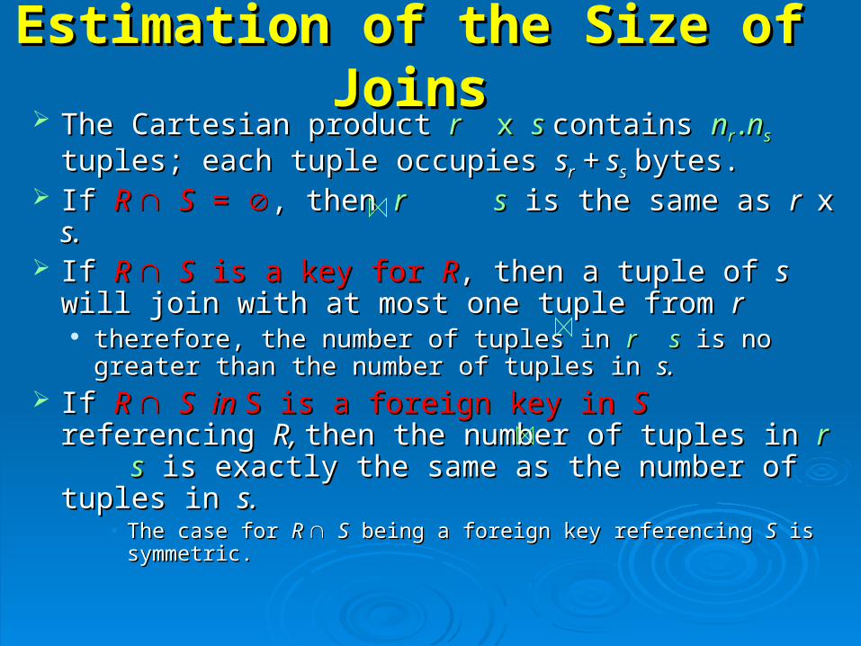
Estimation of the Size of JoinsEstimation of the Size of Joins The Cartesian product The Cartesian product rr x x ss contains contains nnr r .n.nss tuples; tuples;

each tuple occupies each tuple occupies ssrr + s + sss bytes.bytes. If If R R SS = = , then , then rr ss is the same as is the same as r r x x s. s. If If R R SS is a key for is a key for RR, then a tuple of , then a tuple of ss will join with will join with

at most one tuple from at most one tuple from rr therefore, the number of tuples in therefore, the number of tuples in r sr s is no greater than is no greater than

the number of tuples in the number of tuples in s.s. If If R R SS in in S is a foreign keyS is a foreign key in in SS referencing referencing R, R,

then the number of tuples in then the number of tuples in rr ss is exactly the is exactly the same as the number of tuples in same as the number of tuples in s.s.

• The case for The case for R R SS being a foreign key referencing being a foreign key referencing SS is is symmetric.symmetric.

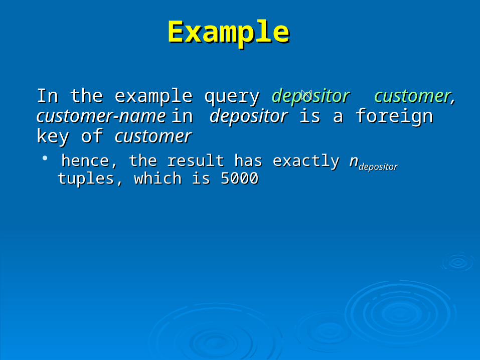
ExampleExample

In the example query In the example query depositor customerdepositor customer, , customer-name customer-name in in depositor depositor is a foreign key of is a foreign key of customercustomer hence, the result has exactly hence, the result has exactly nndepositor depositor tuples, which is tuples, which is

50005000

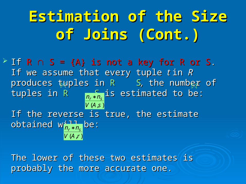
Estimation of the Size of Estimation of the Size of Joins (Cont.)Joins (Cont.)

If If R R S = {A} is not a key for R or S S = {A} is not a key for R or S..If we assume that every tuple If we assume that every tuple t t in in R R produces produces tuples in tuples in R SR S,, the number of tuples in the number of tuples in R SR S is is estimated to be:estimated to be:

If the reverse is true, the estimate obtained will be:If the reverse is true, the estimate obtained will be:

The lower of these two estimates is probably the The lower of these two estimates is probably the more accurate one. more accurate one.

),( sAVnn sr

),( rAVnn sr

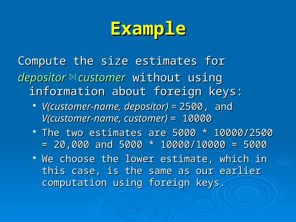
ExampleExample

Compute the size estimates for Compute the size estimates for

depositor customerdepositor customer without using information without using information about foreign keys:about foreign keys: V(customer-name, depositor) = V(customer-name, depositor) = 2500, and2500, and

V(customer-name, customer) V(customer-name, customer) = 10000= 10000 The two estimates are 5000 * 10000/2500 The two estimates are 5000 * 10000/2500 == 20,000 20,000

and 5000 * 10000/10000 = 5000and 5000 * 10000/10000 = 5000 We choose the lower estimate, which in this case, is We choose the lower estimate, which in this case, is

the same as our earlier computation using foreign the same as our earlier computation using foreign keys.keys.

Size Estimation for Projection, Size Estimation for Projection, Aggregation and Outer JoinAggregation and Outer Join

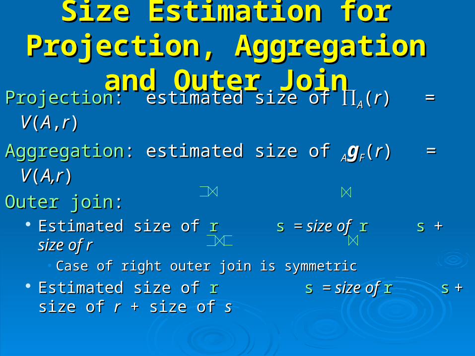
ProjectionProjection: estimated size of : estimated size of AA((rr) = ) = VV((AA,,rr))

AggregationAggregation: estimated size of : estimated size of AAggFF((rr) = ) = VV((A,rA,r))

Outer joinOuter join: : Estimated size of Estimated size of r sr s = size of = size of r sr s + size of r + size of r

• Case of right outer join is symmetricCase of right outer join is symmetric Estimated size of Estimated size of r sr s = size of = size of r sr s + size of + size of rr

+ size of + size of ss

Size Estimation for Set Size Estimation for Set OperationsOperations

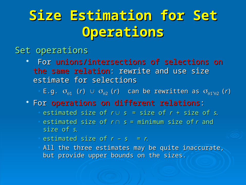
Set operationsSet operations For For unions/intersections of selections on the same unions/intersections of selections on the same

relationrelation: rewrite and use size estimate for selections: rewrite and use size estimate for selections• E.g.E.g. 11 ( (rr) ) 22 ((rr) can be rewritten as ) can be rewritten as 1122 ((rr))

For For operations on different relationsoperations on different relations::• estimated size of estimated size of r r s s = size of = size of rr + size of + size of ss. . • estimated size of estimated size of r r s s = minimum size of= minimum size of r r and size of and size of s.s.• estimated size of estimated size of rr – – s s = = r.r.• All the three estimates may be quite inaccurate, but provide All the three estimates may be quite inaccurate, but provide

upper bounds on the sizes.upper bounds on the sizes.

Estimation of Number of Distinct Estimation of Number of Distinct Values – Selections Values – Selections ((rr) )

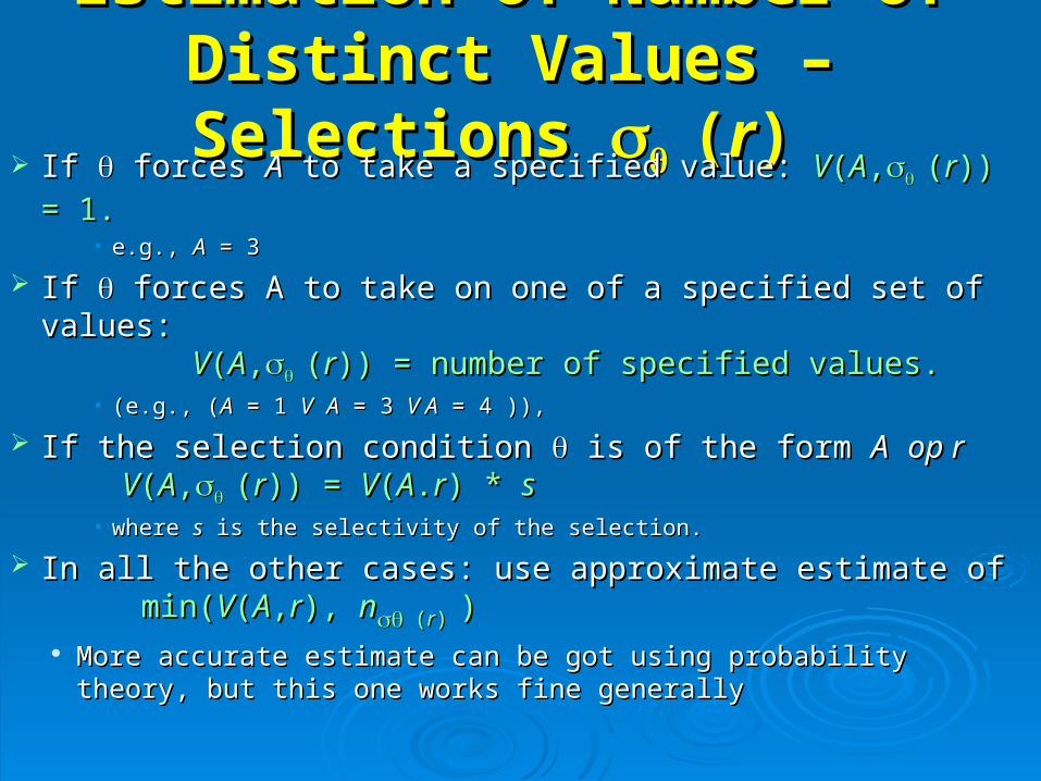
If If forces forces AA to take a specified value: to take a specified value: VV((AA,, ((rr)) = 1.)) = 1.• e.g., e.g., AA = 3 = 3

If If forces A to take on one of a specified set of values: forces A to take on one of a specified set of values: VV((AA,, ((rr)) = number of specified values.)) = number of specified values.

• (e.g., ((e.g., (AA = 1 = 1 VV AA = 3 = 3 V AV A = 4 )), = 4 )),

If the selection condition If the selection condition is of the form is of the form AA op rop rVV((AA,, ((rr)) = )) = VV((AA..rr) * ) * ss

• where where ss is the selectivity of the selection. is the selectivity of the selection.

In all the other cases: use approximate estimate ofIn all the other cases: use approximate estimate of min(min(VV((AA,,rr), ), nn ((rr)) ))

More accurate estimate can be got using probability theory, but More accurate estimate can be got using probability theory, but this one works fine generallythis one works fine generally

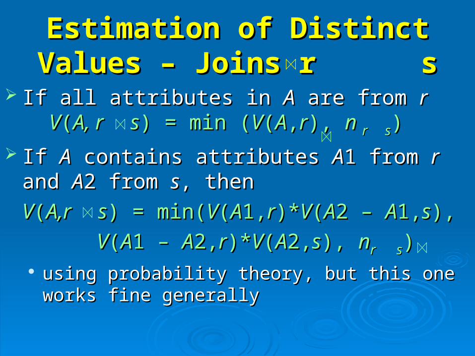
Estimation of Distinct Values Estimation of Distinct Values – Joins r s– Joins r s

If all attributes in If all attributes in AA are from are from rr VV((A, r sA, r s) = min () = min (VV((AA,,rr), ), n n r sr s))

If If AA contains attributes contains attributes AA1 from 1 from rr and and AA2 from 2 from ss, , then then

VV((A,r sA,r s) = min() = min(VV((AA1,1,rr)*)*VV((AA2 – 2 – AA1,1,ss),),

VV((AA1 – 1 – AA2,2,rr)*)*VV((AA2,2,ss), ), nnr sr s)) using probability theory, but this one works fine using probability theory, but this one works fine

generallygenerally

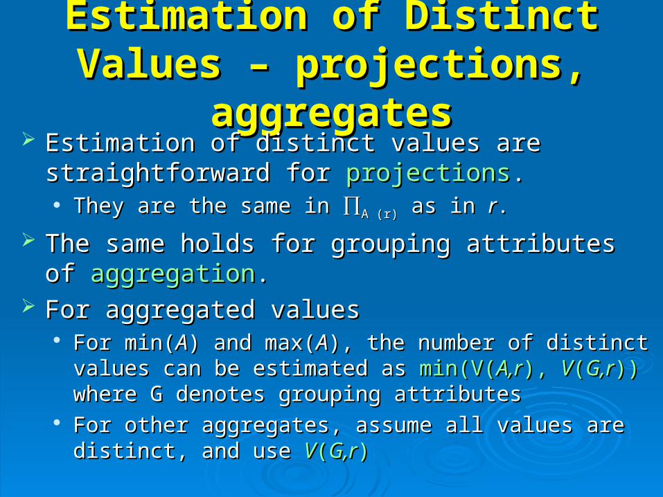
Estimation of Distinct Values Estimation of Distinct Values – projections, aggregates– projections, aggregates

Estimation of distinct values are straightforward for Estimation of distinct values are straightforward for projectionsprojections.. They are the same in They are the same in A (r)A (r) as in as in rr. .

The same holds for grouping attributes of The same holds for grouping attributes of aggregationaggregation..

For aggregated values For aggregated values For min(For min(AA) and max() and max(AA), the number of distinct values can ), the number of distinct values can

be estimated as be estimated as min(V(min(V(A,rA,r), ), VV((G,rG,r)))) where G denotes where G denotes grouping attributesgrouping attributes

For other aggregates, assume all values are distinct, and For other aggregates, assume all values are distinct, and use use VV((G,rG,r))

Transformation of Relational Transformation of Relational ExpressionsExpressions

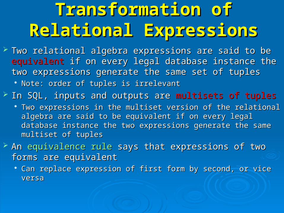
Two relational algebra expressions are said to be Two relational algebra expressions are said to be equivalentequivalent if on every legal database instance the two if on every legal database instance the two expressions generate the same set of tuplesexpressions generate the same set of tuples Note: order of tuples is irrelevantNote: order of tuples is irrelevant

In SQL, inputs and outputs are In SQL, inputs and outputs are multisets of tuplesmultisets of tuples Two expressions in the multiset version of the relational algebra Two expressions in the multiset version of the relational algebra

are said to be equivalent if on every legal database instance the are said to be equivalent if on every legal database instance the two expressions generate the same multiset of tuplestwo expressions generate the same multiset of tuples

An An equivalence ruleequivalence rule says that expressions of two forms are says that expressions of two forms are equivalentequivalent Can replace expression of first form by second, or vice versaCan replace expression of first form by second, or vice versa

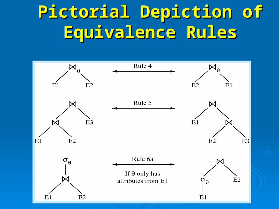
Pictorial Depiction of Pictorial Depiction of Equivalence RulesEquivalence Rules

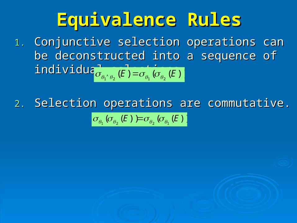
Equivalence RulesEquivalence Rules1.1. Conjunctive selection operations can be Conjunctive selection operations can be

deconstructed into a sequence of individual deconstructed into a sequence of individual selections.selections.

2.2. Selection operations are commutative.Selection operations are commutative.))(())((

1221EE

))(()(2121EE

Equivalence RulesEquivalence Rules

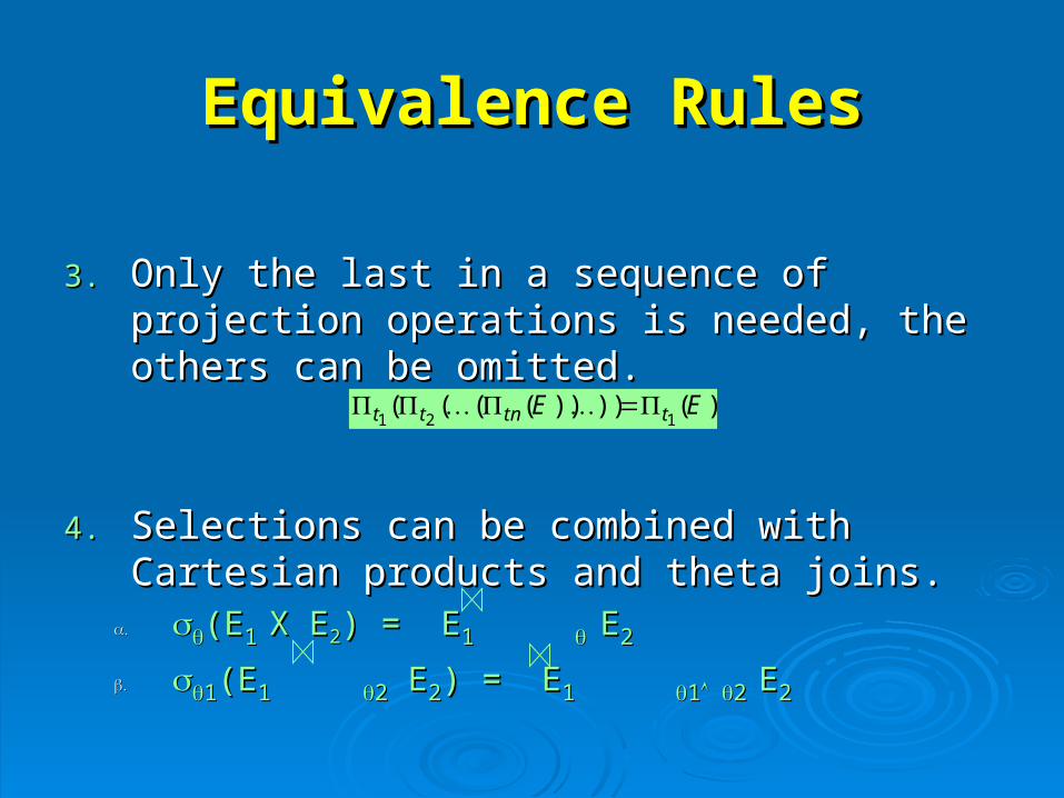
3.3. Only the last in a sequence of projection Only the last in a sequence of projection operations is needed, the others can be omitted.operations is needed, the others can be omitted.

4.4. Selections can be combined with Cartesian Selections can be combined with Cartesian products and theta joins.products and theta joins.

a.a. (E(E11 X EX E22) = E) = E11 EE22

b.b. 11(E(E11 22 E E22) = E) = E11 11 22 EE22

)())))((((121

EE ttntt

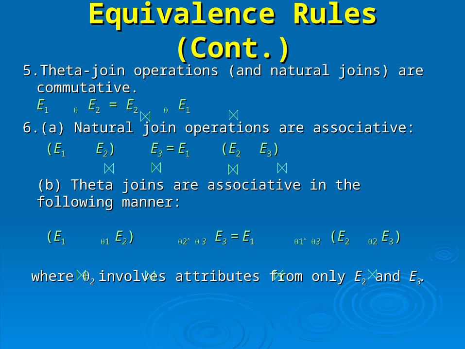
Equivalence Rules (Cont.)Equivalence Rules (Cont.)5.5. Theta-join operations (and natural joins) are Theta-join operations (and natural joins) are

commutative.commutative.EE1 1 EE22 = = EE22 EE11

6.6. (a) Natural join operations are associative:(a) Natural join operations are associative:

((EE1 1 EE22) ) EE33 = E = E1 1 ((EE22 E E33))

(b) Theta joins are associative in the following manner:(b) Theta joins are associative in the following manner:

((EE1 1 1 1 EE22) ) 22 3 3 EE33 = E = E1 1 11 33 ( (EE22 22 E E33))

where where 22 involves attributes from only involves attributes from only EE22 and and EE33..

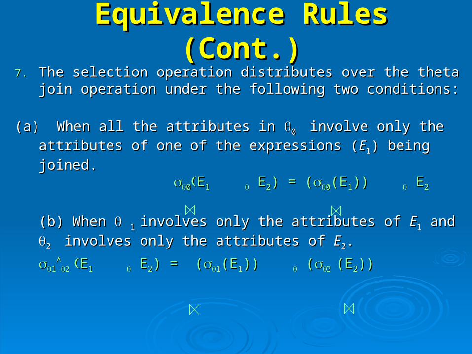
Equivalence Rules (Cont.)Equivalence Rules (Cont.)7.7. The selection operation distributes over the theta join The selection operation distributes over the theta join

operation under the following two conditions:operation under the following two conditions:

(a) When all the attributes in (a) When all the attributes in 0 0 involve only the attributes of involve only the attributes of

one of the expressions (one of the expressions (EE11) being joined.) being joined.

00EE1 1 E E22) = () = (00(E(E11)) )) E E22

(b) When (b) When 1 1 involves only the attributes of involves only the attributes of EE11 and and 2 2

involves only the attributes of involves only the attributes of EE22..

11 EE11 E E22) = () = (11(E(E11)) )) ( ( (E(E22))))

Equivalence Rules (Cont.)Equivalence Rules (Cont.)

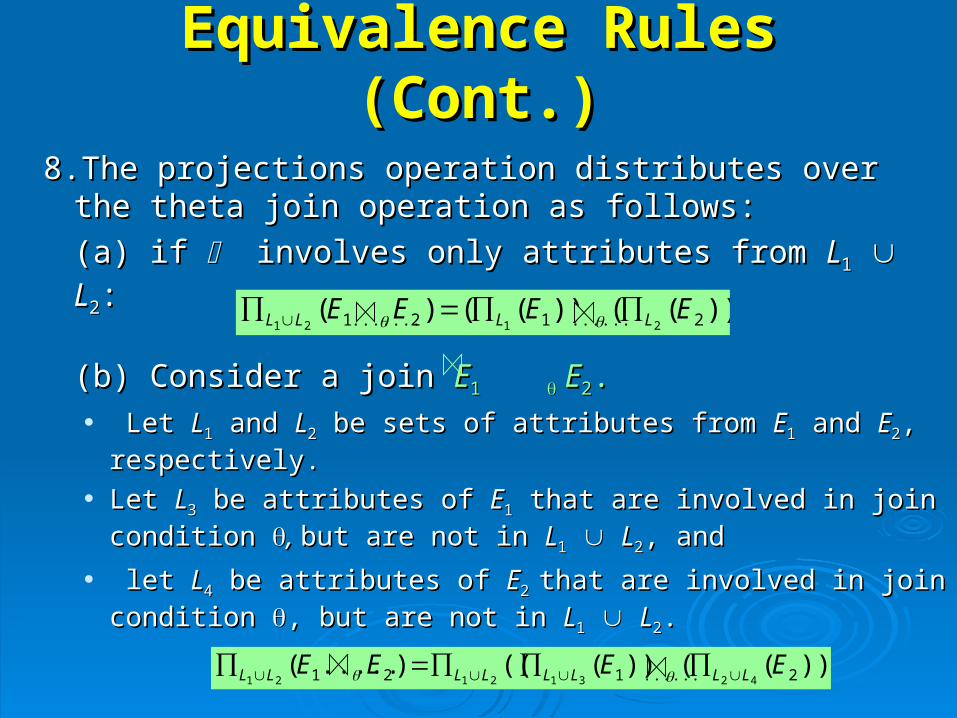
8.8. The projections operation distributes over the theta The projections operation distributes over the theta join operation as follows:join operation as follows:

(a) if (a) if involves only attributes from involves only attributes from LL11 LL22::

(b) Consider a join (b) Consider a join EE1 1 E E22.. Let Let LL11 and and LL22 be sets of attributes from be sets of attributes from EE11 and and EE22, ,

respectively. respectively. Let Let LL33 be attributes of be attributes of EE11 that are involved in join condition that are involved in join condition , ,

but are not in but are not in LL11 LL22, and, and

let let LL44 be attributes of be attributes of EE2 2 that are involved in join condition that are involved in join condition , , but are not in but are not in LL11 LL22..

))(())(()( 2......12.......1 2121EEEE LLLL

)))(())((().....( 2......121 42312121EEEE LLLLLLLL

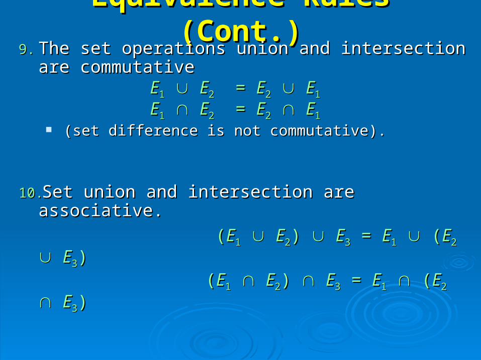
Equivalence Rules (Cont.)Equivalence Rules (Cont.)9.9. The set operations union and intersection are The set operations union and intersection are

commutative commutative EE11 EE22 = = EE22 EE11 EE11 EE22 = = EE22 EE11

(set difference is not commutative).(set difference is not commutative).

10.10.Set union and intersection are associative.Set union and intersection are associative.

((EE11 EE22) ) EE33 = = EE11 ( (EE22 EE33)) ((EE11 EE22) ) EE33 = = EE11 ( (EE22 EE33))

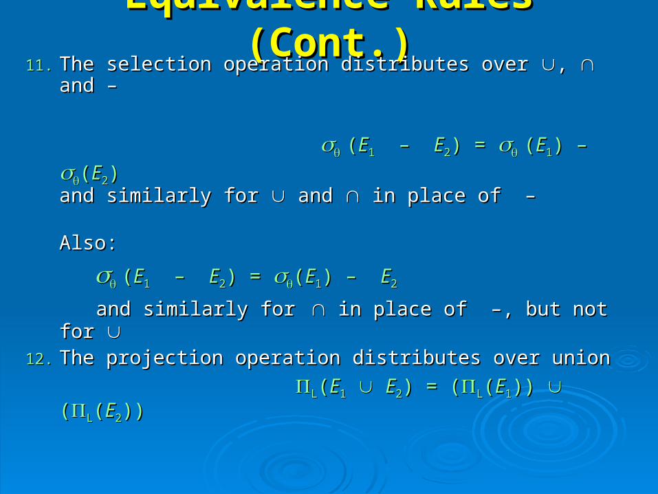
Equivalence Rules (Cont.)Equivalence Rules (Cont.)11.11. The selection operation distributes over The selection operation distributes over , , and and

––

((EE11 – – EE22) = ) = ((EE11) – ) – ((EE22))and similarly for and similarly for and and in place of – in place of –

Also: Also:

((EE11 – – EE22) = ) = ((EE11) – ) – EE22

and similarly forand similarly for in place of –, but not for in place of –, but not for 12.12. The projection operation distributes over unionThe projection operation distributes over union

LL((EE11 EE22) = () = (LL((EE11)) )) ( (LL((EE22)) ))

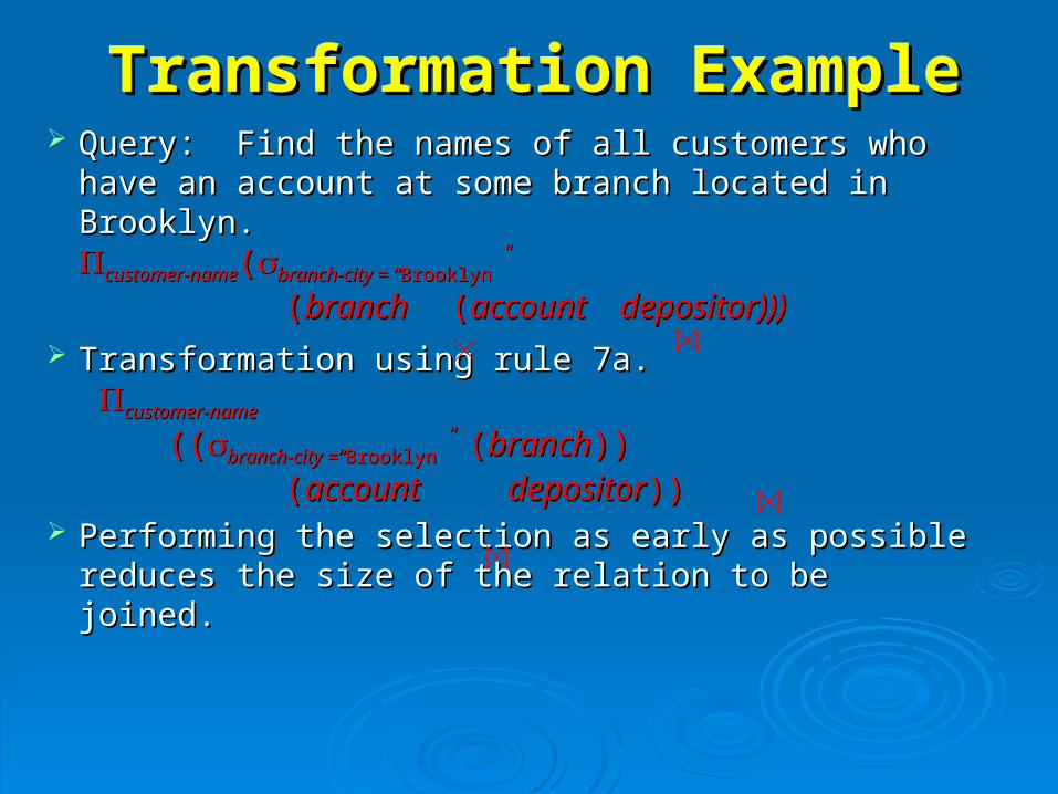
Transformation ExampleTransformation Example Query: Find the names of all customers who have Query: Find the names of all customers who have

an account at some branch located in Brooklyn.an account at some branch located in Brooklyn.customer-namecustomer-name((branch-city = “branch-city = “Brooklyn”Brooklyn”

((branch branch ((account depositor)))account depositor)))

Transformation using rule 7a.Transformation using rule 7a. customer-namecustomer-name

((((branch-city =“branch-city =“Brooklyn”Brooklyn” ( (branchbranch))))

((account account depositordepositor)))) Performing the selection as early as possible Performing the selection as early as possible

reduces the size of the relation to be joined. reduces the size of the relation to be joined.

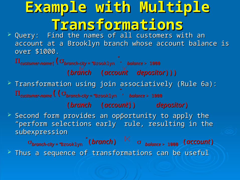
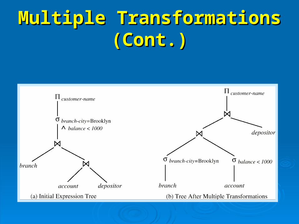
Example with Multiple Example with Multiple TransformationsTransformations

Query: Find the names of all customers with an account at a Query: Find the names of all customers with an account at a Brooklyn branch whose account balance is over $1000.Brooklyn branch whose account balance is over $1000.

customer-namecustomer-name((((branch-city = “branch-city = “Brooklyn” Brooklyn” balance balance > 1000> 1000

((branch branch ((account depositoraccount depositor)))))) Transformation using join associatively (Rule 6a):Transformation using join associatively (Rule 6a):

customer-namecustomer-name((((branch-city = “branch-city = “Brooklyn” Brooklyn” balance balance > 1000> 1000

((branch branch ((accountaccount)) )) depositordepositor)) Second form provides an opportunity to apply the “perform Second form provides an opportunity to apply the “perform

selections early” rule, resulting in the subexpressionselections early” rule, resulting in the subexpression

branch-city = “branch-city = “Brooklyn”Brooklyn” ((branchbranch) ) balance balance > 1000> 1000 ( (accountaccount))

Thus a sequence of transformations can be usefulThus a sequence of transformations can be useful

Multiple Transformations Multiple Transformations (Cont.)(Cont.)

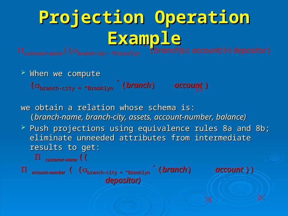
Projection Operation ExampleProjection Operation Example

When we computeWhen we compute

((branch-city = “Brooklyn”branch-city = “Brooklyn” ( (branchbranch) ) account account ))

we obtain a relation whose schema is:we obtain a relation whose schema is:((branch-name, branch-city, assets, account-number, balance)branch-name, branch-city, assets, account-number, balance)

Push projections using equivalence rules 8a and 8b; eliminate Push projections using equivalence rules 8a and 8b; eliminate unneeded attributes from intermediate results to get:unneeded attributes from intermediate results to get: customer-name customer-name (( ((

account-numberaccount-number ( (( (branch-city = “Brooklyn”branch-city = “Brooklyn” ( (branchbranch) ) account account )) ))

depositor)depositor)

customer-name((branch-city = “Brooklyn” (branch) account) depositor)

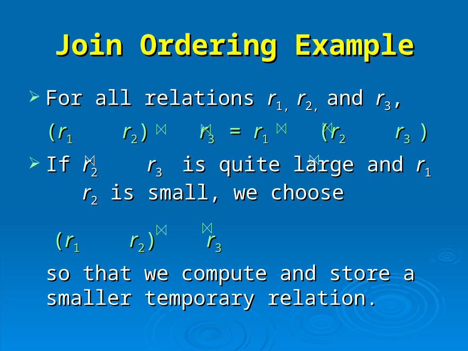
Join Ordering ExampleJoin Ordering Example

For all relations For all relations rr1, 1, rr2, 2, and and rr33,,

((rr11 rr22) ) rr3 3 = = rr11 ( (rr22 rr3 3 ))

If If rr22 rr3 3 is quite large and is quite large and rr11 rr22 is small, is small,

we choosewe choose

((rr11 rr22) ) rr3 3

so that we compute and store a smaller so that we compute and store a smaller temporary relation.temporary relation.

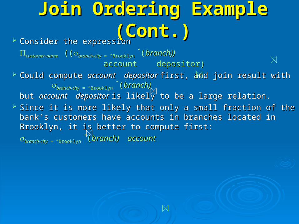
Join Ordering Example (Cont.)Join Ordering Example (Cont.) Consider the expressionConsider the expression

customer-namecustomer-name ((((branch-citybranch-city = “Brooklyn” = “Brooklyn” ((branch))branch))

account depositor)account depositor) Could compute Could compute account depositor account depositor first, and join result with first, and join result with

branch-citybranch-city = “Brooklyn” = “Brooklyn” ((branch)branch)

but but account depositor account depositor is likely to be a large relation.is likely to be a large relation. Since it is more likely that only a small fraction of the bank’s customers Since it is more likely that only a small fraction of the bank’s customers

have accounts in branches located in Brooklyn, it is better to compute first:have accounts in branches located in Brooklyn, it is better to compute first:

branch-citybranch-city = “Brooklyn” = “Brooklyn” ((branch) accountbranch) account

Enumeration of Equivalent Enumeration of Equivalent ExpressionsExpressions

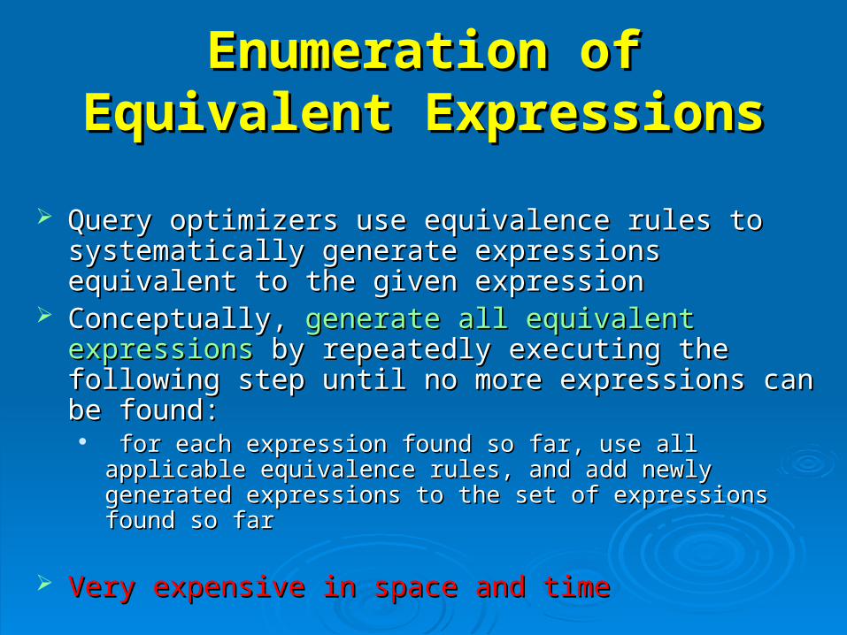
Query optimizers use equivalence rules to systematically Query optimizers use equivalence rules to systematically generate expressions equivalent to the given expressiongenerate expressions equivalent to the given expression

Conceptually, Conceptually, generate all equivalent expressionsgenerate all equivalent expressions by by repeatedly executing the following step until no more repeatedly executing the following step until no more expressions can be found: expressions can be found: for each expression found so far, use all applicable equivalence for each expression found so far, use all applicable equivalence

rules, and add newly generated expressions to the set of rules, and add newly generated expressions to the set of expressions found so farexpressions found so far

Very expensive in space and timeVery expensive in space and time

Enumeration of Equivalent Enumeration of Equivalent Expressions (cont.)Expressions (cont.)

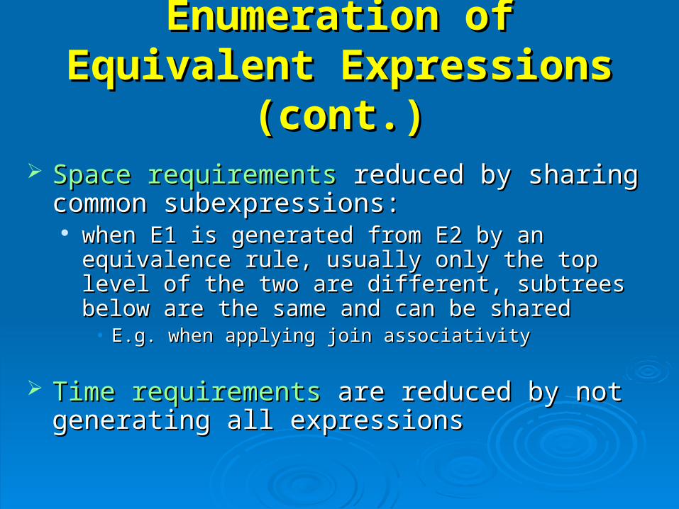
Space requirementsSpace requirements reduced by sharing common reduced by sharing common subexpressions:subexpressions: when E1 is generated from E2 by an equivalence rule, when E1 is generated from E2 by an equivalence rule,

usually only the top level of the two are different, usually only the top level of the two are different, subtrees below are the same and can be sharedsubtrees below are the same and can be shared

• E.g. when applying join associativityE.g. when applying join associativity

Time requirementsTime requirements are reduced by not generating are reduced by not generating all expressionsall expressions

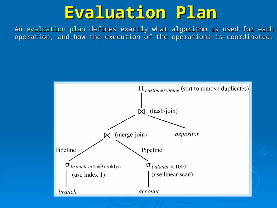
Evaluation PlanEvaluation PlanAn An evaluation planevaluation plan defines exactly what algorithm is used for each defines exactly what algorithm is used for each operation, and how the execution of the operations is coordinated.operation, and how the execution of the operations is coordinated.

Choice of Evaluation PlansChoice of Evaluation Plans Must consider the Must consider the interaction of evaluation techniques when interaction of evaluation techniques when

choosing evaluation planschoosing evaluation plans: choosing the cheapest algorithm : choosing the cheapest algorithm for each operation independently may not yield best overall for each operation independently may not yield best overall algorithm. E.g.algorithm. E.g. merge-join may be costlier than hash-join, but may provide a sorted merge-join may be costlier than hash-join, but may provide a sorted

output which reduces the cost for an outer level aggregation.output which reduces the cost for an outer level aggregation. nested-loop join may provide opportunity for pipeliningnested-loop join may provide opportunity for pipelining

Practical query optimizersPractical query optimizers incorporate elements of the incorporate elements of the following two broad approaches:following two broad approaches:1.1. Search all the plans and choose the best plan in a Search all the plans and choose the best plan in a

cost-based fashioncost-based fashion..

2. Uses 2. Uses heuristicsheuristics to choose a plan. to choose a plan.

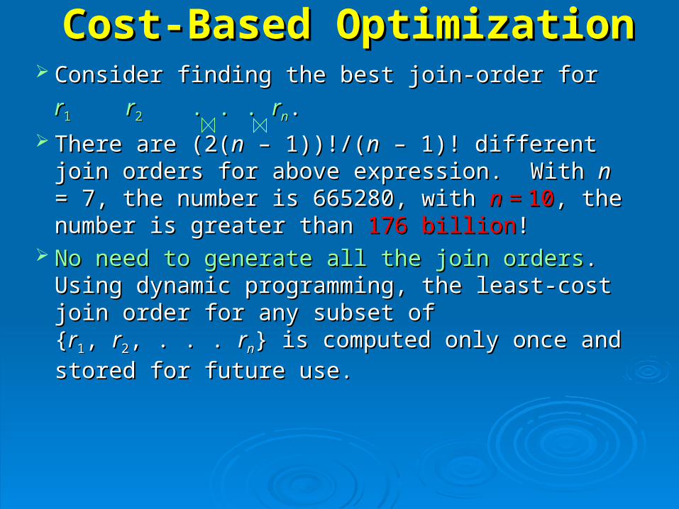
Cost-Based OptimizationCost-Based Optimization Consider finding the best join-order for Consider finding the best join-order for

rr11 rr2 2 . . . . . . rrnn..

There are (2(There are (2(nn – 1))!/( – 1))!/(nn – 1)! different join orders for – 1)! different join orders for above expression. With above expression. With nn = 7, the number is 665280, = 7, the number is 665280, with with n = n = 1010, the, the number is greater than number is greater than 176 billion176 billion!!

No need to generate all the join ordersNo need to generate all the join orders. Using . Using dynamic programming, the least-cost join order for any dynamic programming, the least-cost join order for any subset of subset of {{rr11, , rr22, . . . , . . . rrnn} is computed only once and stored for } is computed only once and stored for

future use. future use.

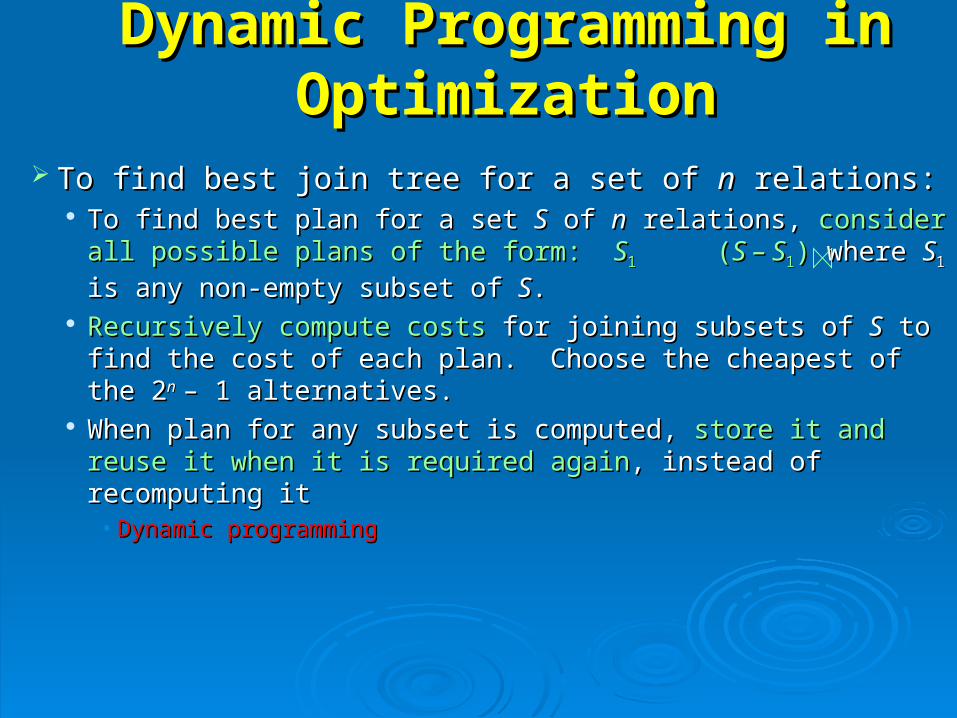
Dynamic Programming in Dynamic Programming in OptimizationOptimization

To find best join tree for a set of To find best join tree for a set of nn relations: relations: To find best plan for a set To find best plan for a set SS of of nn relations, relations, consider all consider all

possible plans of the form: possible plans of the form: SS11 ( (S – SS – S11)) where where SS11 is any is any

non-empty subset of non-empty subset of SS.. Recursively compute costsRecursively compute costs for joining subsets of for joining subsets of SS to find the to find the

cost of each plan. Choose the cheapest of the 2cost of each plan. Choose the cheapest of the 2nn – 1 – 1 alternatives.alternatives.

When plan for any subset is computed, When plan for any subset is computed, store it and reuse it store it and reuse it when it is required againwhen it is required again, instead of recomputing it, instead of recomputing it• Dynamic programmingDynamic programming

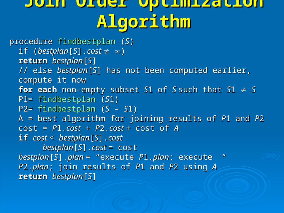
Join Order Optimization AlgorithmJoin Order Optimization Algorithm

procedure procedure findbestplan findbestplan ((SS))if (if (bestplanbestplan[[SS].].cost cost ))

return return bestplanbestplan[[SS]]// else // else bestplanbestplan[[SS] has not been computed earlier, compute it ] has not been computed earlier, compute it nownowfor each for each non-empty subset non-empty subset SS1 of 1 of S S such that such that SS1 1 SS

P1= P1= findbestplanfindbestplan ( (SS1)1)P2= P2= findbestplanfindbestplan ( (SS - - SS1)1)A = best algorithm for joining results of A = best algorithm for joining results of PP1 and 1 and PP22cost = cost = PP1.1.costcost + + PP2.2.cost cost + cost of + cost of AAif if cost cost < < bestplanbestplan[[SS].].cost cost

bestplanbestplan[[SS].].cost cost = cost= costbestplanbestplan[[SS].].plan plan = “execute = “execute PP1.1.planplan; execute ; execute PP2.2.planplan; join results of ; join results of PP1 and 1 and PP2 using 2 using AA””

returnreturn bestplanbestplan[[SS]]

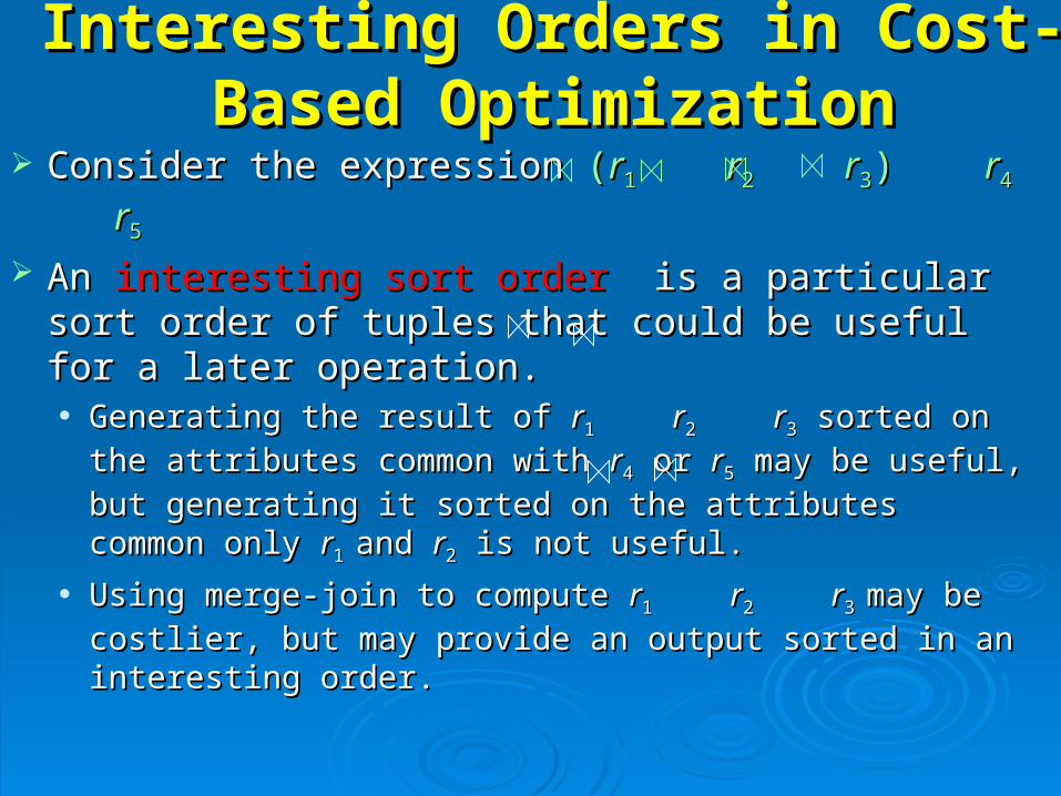
Interesting Orders in Cost-Based Interesting Orders in Cost-Based OptimizationOptimization

Consider the expression Consider the expression ((rr11 rr22 rr33) ) rr44 rr55

An An interesting sort orderinteresting sort order is a particular sort order of is a particular sort order of tuples that could be useful for a later operation.tuples that could be useful for a later operation. Generating the result of Generating the result of rr11 rr22 rr33 sorted on the attributes sorted on the attributes

common with common with rr44 or or rr55 may be useful, but generating it sorted may be useful, but generating it sorted

on the attributes common only on the attributes common only rr1 1 and and rr22 is not useful. is not useful.

Using merge-join to compute Using merge-join to compute rr11 rr22 rr3 3 may be costlier, but may be costlier, but

may provide an output sorted in an interesting order.may provide an output sorted in an interesting order.

Interesting Orders in Cost-Based Interesting Orders in Cost-Based Optimization (cont.)Optimization (cont.)

Not sufficient to find the best join order for each Not sufficient to find the best join order for each subset of the set of subset of the set of nn given relations; given relations; must find the must find the best join order for each subset, for each interesting best join order for each subset, for each interesting sort ordersort order Simple extension of earlier dynamic programming Simple extension of earlier dynamic programming

algorithmsalgorithms Usually, number of interesting orders is quite small and Usually, number of interesting orders is quite small and

doesn’t affect time/space complexity significantlydoesn’t affect time/space complexity significantly

Heuristic OptimizationHeuristic Optimization Cost-based optimization is expensive, even with dynamic Cost-based optimization is expensive, even with dynamic

programming so systems may use programming so systems may use heuristicsheuristics to reduce the number of to reduce the number of choices that must be made in a cost-based fashion.choices that must be made in a cost-based fashion.

Heuristic optimization transforms the query-tree by using a Heuristic optimization transforms the query-tree by using a set of rules set of rules that typically (but not in all cases) improve execution performancethat typically (but not in all cases) improve execution performance:: Perform selection early (reduces the number of tuples)Perform selection early (reduces the number of tuples) Perform projection early (reduces the number of attributes)Perform projection early (reduces the number of attributes) Perform most restrictive selection and join operations before other similar Perform most restrictive selection and join operations before other similar

operations.operations. Some systems use only heuristics, others combine heuristics with partial cost-Some systems use only heuristics, others combine heuristics with partial cost-

based optimization.based optimization.

Steps in Typical Heuristic Steps in Typical Heuristic OptimizationOptimization

1.1. Deconstruct conjunctive selections into a sequence of single Deconstruct conjunctive selections into a sequence of single selection operations (Equiv. rule 1.).selection operations (Equiv. rule 1.).

2.2. Move selection operations down the query tree for the earliest Move selection operations down the query tree for the earliest possible execution (Equiv. rules 2, 7a, 7b, 11).possible execution (Equiv. rules 2, 7a, 7b, 11).

3.3. Execute first those selection and join operations that will Execute first those selection and join operations that will produce the smallest relations (Equiv. rule 6).produce the smallest relations (Equiv. rule 6).

4.4. Replace Cartesian product operations that are followed by a Replace Cartesian product operations that are followed by a selection condition by join operations (Equiv. rule 4a).selection condition by join operations (Equiv. rule 4a).

5.5. Deconstruct and move as far down the tree as possible lists of Deconstruct and move as far down the tree as possible lists of projection attributes, creating new projections where needed projection attributes, creating new projections where needed (Equiv. rules 3, 8a, 8b, 12).(Equiv. rules 3, 8a, 8b, 12).

6.6. Identify those subtrees whose operations can be pipelined, Identify those subtrees whose operations can be pipelined, and execute them using pipelining.and execute them using pipelining.

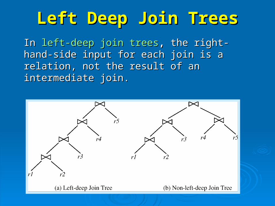
Left Deep Join TreesLeft Deep Join Trees

In In left-deep join treesleft-deep join trees,, the right-hand-side the right-hand-side input for each join is a relation, not the input for each join is a relation, not the result of an intermediate join.result of an intermediate join.

Cost of OptimizationCost of Optimization With dynamic programming With dynamic programming time complexity of optimization with time complexity of optimization with

bushy treesbushy trees is is OO(3(3nn). ). With With n n = 10, this number is 59000 instead of 176 billion!= 10, this number is 59000 instead of 176 billion!

Space complexitySpace complexity is is OO(2(2nn) ) To To find best left-deep join treefind best left-deep join tree for a set of for a set of nn relations: relations:

Consider Consider n n alternatives with one relation as right-hand side input and the alternatives with one relation as right-hand side input and the other relations as left-hand side input.other relations as left-hand side input.

Using (recursively computed and stored) least-cost join order for each Using (recursively computed and stored) least-cost join order for each alternative on left-hand-side, choose the cheapest of the alternative on left-hand-side, choose the cheapest of the nn alternatives. alternatives.

If If only left-deep trees are consideredonly left-deep trees are considered, time complexity of finding , time complexity of finding best join order is best join order is OO((n n 22nn)) Space complexity remains at Space complexity remains at OO(2(2nn) )

Cost-based optimization is expensive, but worthwhile for queries Cost-based optimization is expensive, but worthwhile for queries on large datasets (typical queries have small n, generally < 10)on large datasets (typical queries have small n, generally < 10)

Structure of Query OptimizersStructure of Query Optimizers

The The System R/StarburstSystem R/Starburst optimizer considers only optimizer considers only left-deep join left-deep join ordersorders. This reduces optimization complexity and generates . This reduces optimization complexity and generates plans amenable to pipelined evaluation.plans amenable to pipelined evaluation. also uses heuristics to push selections and projections down the query also uses heuristics to push selections and projections down the query

tree.tree.

Heuristic optimization used in some versions of Heuristic optimization used in some versions of OracleOracle:: Repeatedly pick “best” relation to join next Repeatedly pick “best” relation to join next

• Starting from each of n starting points. Pick best among these.Starting from each of n starting points. Pick best among these.

For For scans using secondary indicesscans using secondary indices, some optimizers take into , some optimizers take into account the probability that the page containing the tuple is in account the probability that the page containing the tuple is in the buffer.the buffer.

Intricacies of SQL complicate query optimizationIntricacies of SQL complicate query optimization E.g. nested subqueriesE.g. nested subqueries

Structure of Query Optimizers Structure of Query Optimizers (Cont.)(Cont.)

Some query optimizers integrate heuristic selection and Some query optimizers integrate heuristic selection and the generation of alternative access plans.the generation of alternative access plans. System R and Starburst use a hierarchical procedure based on System R and Starburst use a hierarchical procedure based on

the nested-block concept of SQL: heuristic rewriting followed the nested-block concept of SQL: heuristic rewriting followed by cost-based join-order optimization.by cost-based join-order optimization.

Even with the use of heuristics, cost-based query Even with the use of heuristics, cost-based query optimization imposes a substantial overhead.optimization imposes a substantial overhead.

This expense is usually more than offset by savings at This expense is usually more than offset by savings at query-execution time, particularly by reducing the query-execution time, particularly by reducing the number of slow disk accesses. number of slow disk accesses.