Ch13 - NLP,DP,GP2005

1

Nonlinear Models:Dynamic, Goal and Nonlinear Programming

Chapter 13

2

13.1 Introduction to Nonlinear Programming

Most real-life situations are more accurately depicted by nonlinear models than by linear models.

Nonlinear models formulated in this chapter fall into three broad categories: Dynamic programming models (DP). Goal programming models (GP). General nonlinear programming models

(NLP).

3

13.2 Dynamic Programming Dynamic programming problems can be thought

of as multistage problems, in which decisions are made “in sequence.”

Known applications of dynamic programming in business: Resource allocation, Equipment replacement, Production and inventory control, Reliability.

4

13.2 Dynamic Programming At stage n a system is found to be in a certain

state. A decision made at stage n takes the system to

stage n+1, and leaves it in a new state for a stage-state related cost/profit.

The decision maker’s challenge is to find a set of optimal decisions for the entire process.

5

13.5 Goal Programming In real life decision situations, virtually all

problems have several objectives. When objectives are conflicting, the

optimal decision is not obvious. Goal programming is an approach that

seeks to simultaneously take into account several objectives.

6

Goals are prioritized in some sense, and their level of aspiration is stated.

An optimal solution is attained when all the goals are reached as close as possible to their aspiration level, while satisfying a set of constraints.

There are two types of goal programming models: Nonpreemtive goal programming - no goal is pre-determined to

dominate any other goal. Preemtive goal programming - goals are assigned different priority

levels. Level 1 goal dominates level 2 goal, and so on.

13.5 Goal Programming

7

13.6 Nonlinear Programming

A nonlinear programming problem (NLP) is one in which the objective function, F, and or one or more constraint functions, Gi, possess nonlinear terms.

There is no a universal algorithm that can find the optimal solution to every NLP.

One class of NLPs “Convex Programming Problems” can be solved by algorithms that are guaranteed to converge to the optimal solution.

8

The objective is to maximize a concave function or to minimize a convex function.

The set of constraints form a convex set.

Properties of Convex Programming Problems

9

A smooth function (no sharp points, no discontinuities)

One global maximum (minimum). A line drawn between any two points on the

curve of the function will lie below (above) the curve or on the curve.

A One Variable Concave (Convex) Function

X

A Concave function

A convex function

X

10

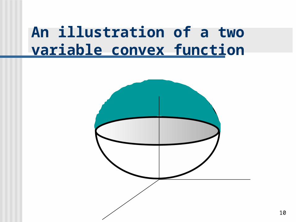
An illustration of a two variable convex function

11

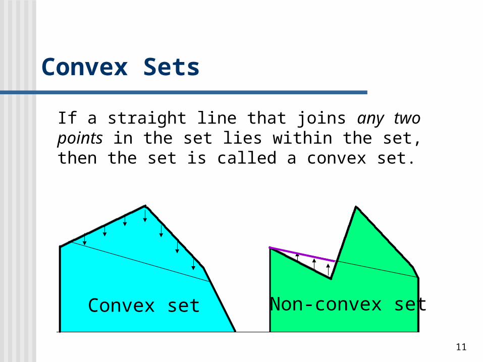
If a straight line that joins any two points in the set lies within the set, then the set is called a convex set.

Convex set Non-convex set

Convex Sets

12

In a NLP model all the constraints are of the “less than or equal to” form Gi(X) B.

If all the functions Gi are convex, the set of constraints forms a convex set.

NLP and Convex Sets

13

Constrained Unconstrained

Types of NLP

14

Dynamic ProgrammingUS Department of Labour

Goal ProgrammingAdvertisement example

Non Linear ProgrammingToshi CameraPBI

Examples for NLP Problems

15

THE U.S. DEPARTMENT OF LABOR(example for a dynamic programming problem)

16

The U.S. Department of Labor has made up to $5 million available to the city of Houston for job creation.

Requests for funding are to be prepared by four Requests for funding are to be prepared by four departments.departments.

The Department of Labor would like to allocate funds to maximize the number of jobs created.

THE U.S. DEPARTMENT OF LABOR

17

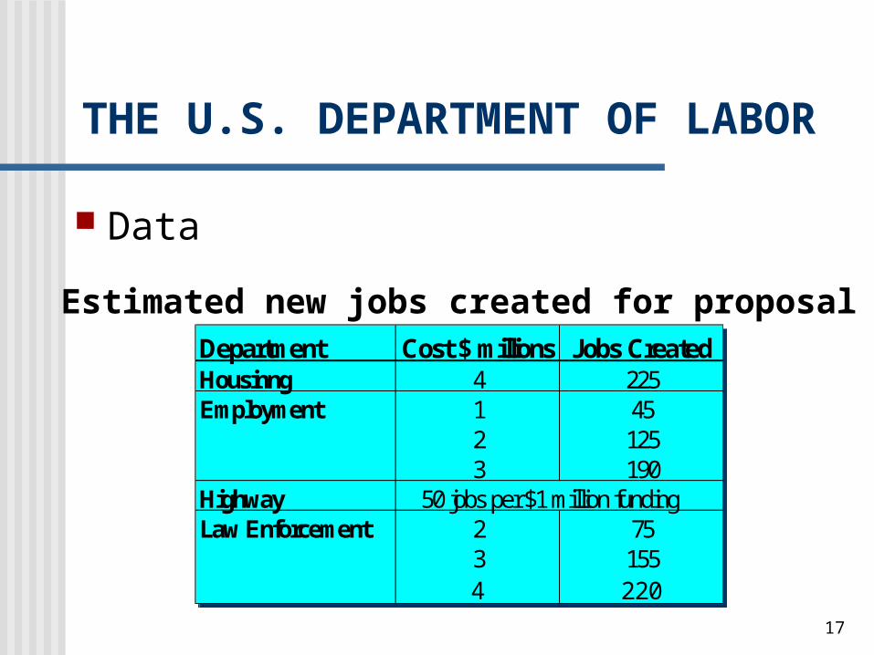
Data

Department Cost $ millions Jobs CreatedHousinng 4 225Employment 1 45

2 1253 190

Highway 50 jobs per $1 million fundingLaw Enforcement 2 75

3 1554 220

Estimated new jobs created for proposal

THE U.S. DEPARTMENT OF LABOR

18

SOLUTION

The U.S. Department of Labor wants to:

Maximize the total number of new jobs.

Limit funding to $5 million.

Fund at most one proposal from each department

19

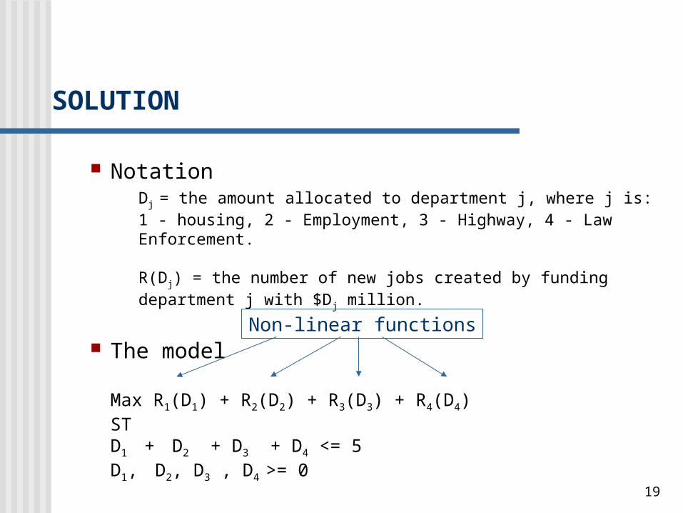
Notation Dj = the amount allocated to department j, where j is:1 - housing, 2 - Employment, 3 - Highway, 4 - Law Enforcement.

R(Dj) = the number of new jobs created by funding department j with $Dj million.

The model

Max R1(D1) + R2(D2) + R3(D3) + R4(D4) STD1 + D2 + D3 + D4 <= 5D1, D2, D3 , D4 >= 0

Non-linear functions

SOLUTION

20

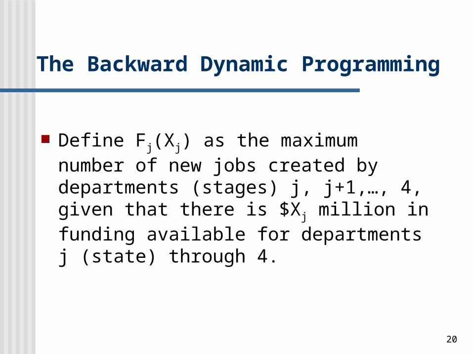
Define Fj(Xj) as the maximum number of new jobs created by departments (stages) j, j+1,…, 4, given that there is $Xj million in funding available for departments j (state) through 4.

The Backward Dynamic Programming

21

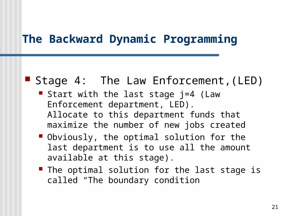
Stage 4: The Law Enforcement,(LED) Start with the last stage j=4 (Law Enforcement

department, LED).Allocate to this department funds that maximize the number of new jobs created

Obviously, the optimal solution for the last department is to use all the amount available at this stage).

The optimal solution for the last stage is called “The boundary condition

The Backward Dynamic Programming

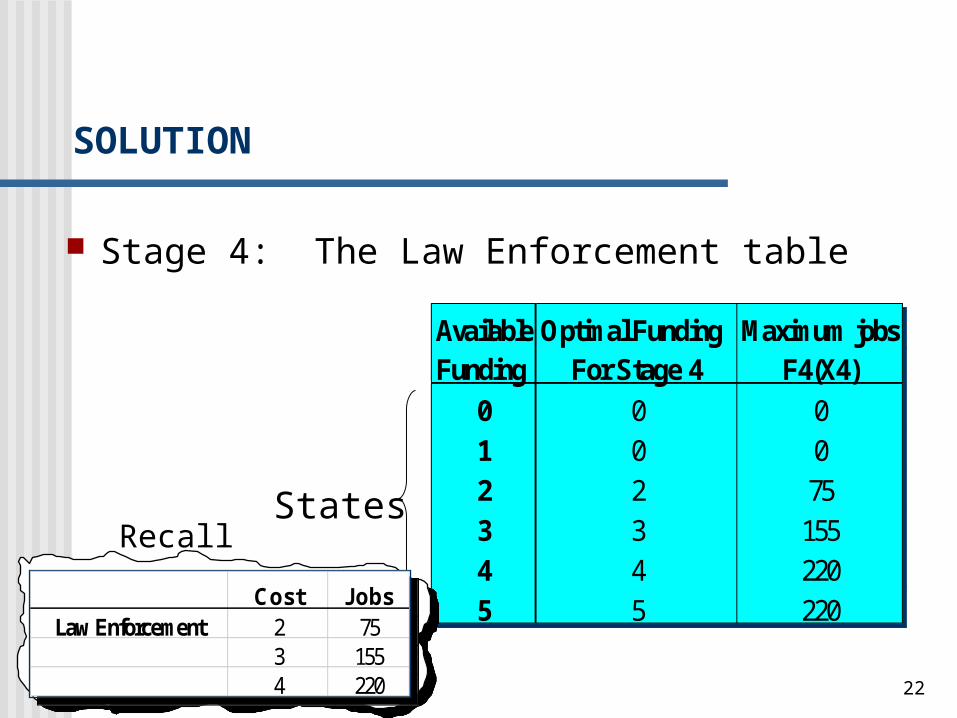
22

Stage 4: The Law Enforcement table

Available Optimal Funding Maximum jobsFunding For Stage 4 F4(X4)

0 0 01 0 02 2 753 3 1554 4 2205 5 220

States

Cost JobsLaw Enforcement 2 75

3 1554 220

Recall

SOLUTION

23

Stage 3: The Highway Department, (HD) At this stage we consider the funding of both the

Highway department and the Law Enforcement department.

For a given amount of funds available for funding of these two departments, the decision regarding the funds allocated to the HD affects the funds available for the LED).

SOLUTION

24

Available Possible Remaining Max. New Jobs Optimal F3(X3)Funding Funding Funds for When Allocatingfor Stage 3,4 for Stage 3 Stage 4 D3 to Stage 3 Optimal D3

(X3) (D3) (X3-D3) R3(D3)+F4(X3-D3)0 0 0 0 + 0 F3(0) = 0; D3(0) = 01 0 1 0+0

1 0 50+0 = 50 F3(1) = 50; D3 = 1 2 0 2 0+75 = 75

1 1 50+0 = 502 0 100+0 F3(3) = 100; D3 = 2

3 0 3 0+155 = 1551 2 50+75 = 1252 1 100+0 = 1003 0 150+0 = 150 F3(3) = 155; D3 = 0

Stage 3: The Highway Department table

SOLUTION

25

Available Possible Remaining Max. New Jobs Optimal F3(X3)Funding Funding Funds for When Allocatingfor Stage 3,4 for Stage 3 Stage 4 D3 to Stage 3 Optimal D3

(X3) (D3) (X3-D3) R3(D3)+F4(X3-D3)4 0 4 0+220 = 220

1 3 50+155 = 2052 2 100+75 = 1753 1 150+ 0 = 1504 0 200+ 0 = 220 F3(4) = 220; D3 = 0

5 0 5 0+220 = 2201 4 50+220 = 2702 3 100+155 = 2553 2 150+75 = 2254 1 200+0 = 2005 0 250+0 = 250 F3(5) = 270; D3 = 1

SOLUTION

Stage 3: The Highway Department table

26

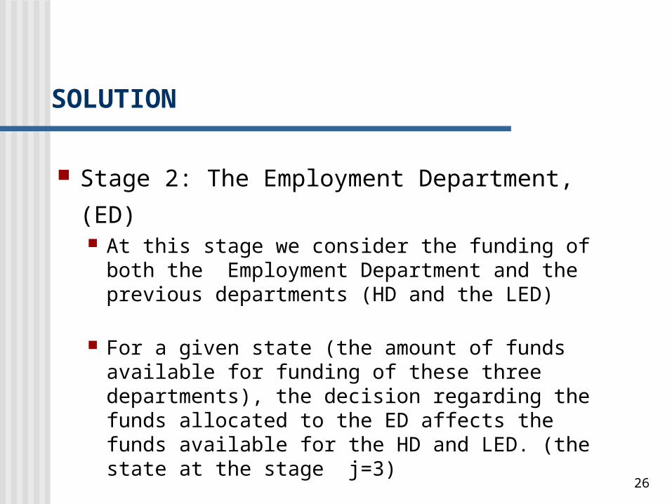
Stage 2: The Employment Department, (ED) At this stage we consider the funding of both the

Employment Department and the previous departments (HD and the LED)

For a given state (the amount of funds available for funding of these three departments), the decision regarding the funds allocated to the ED affects the funds available for the HD and LED. (the state at the stage j=3)

SOLUTION

27

Funding Funding Funds for When Allocatingfor Stage 2,3,4 for Stage 2 Stage 3,4 D2 to Stage 2 Optimal D2

(X2) (D2) (X2-D2) R2(D2)+F3(X2-X2)0 0 0 0 + 0 F2(0) = 0; D2 = 01 0 1 0+50 = 50

1 0 45+0 = 45 F2(1) = 50; D2 = 0 2 0 2 0+100 = 100

1 1 45+50 = 952 0 125+0 = 125 F2(2) = 125; D2 = 2

3 0 3 0+155 = 1551 2 45+100 = 1452 1 125+50 = 1753 0 190+0 = 190 F2(3) = 190; D2 = 3

4 0 4 0+220 = 2201 3 45+155 = 1952 2 125+100 = 2253 1 190+50 = 240 F2(4) = 240; D2 = 3

5 0 5 0+270 = 2701 4 45+220 = 2652 3 125+155 = 2803 2 190+100 = 290 F2(5) = 290; D2 = 3

SOLUTION

28

Stage 1: The Housing Department

At this stage we consider the funding for the Housing Department and all previous departments.

Note that at stage 1 we know there is exactly $5 million to allocate (X1 = 5).

SOLUTION

29

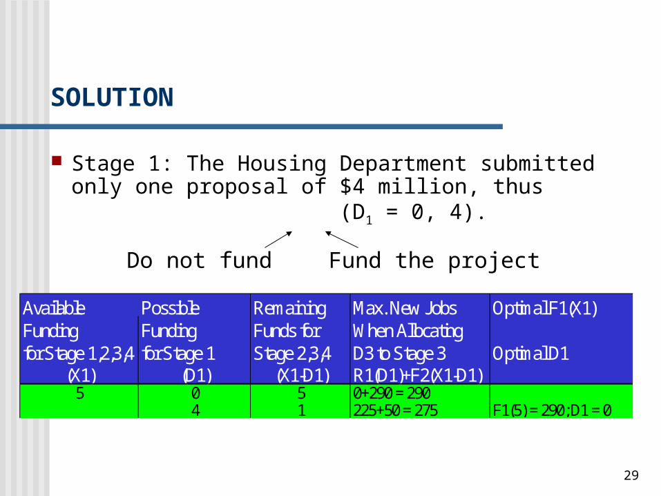
Stage 1: The Housing Department submitted only one proposal of $4 million, thus (D1 = 0, 4).

Available Possible Remaining Max. New Jobs Optimal F1(X1)Funding Funding Funds for When Allocatingfor Stage 1,2,3,4 for Stage 1 Stage 2,3,4 D3 to Stage 3 Optimal D1

(X1) (D1) (X1-D1) R1(D1)+F2(X1-D1)5 0 5 0+290 = 290

4 1 225+50 = 275 F1(5) = 290; D1 = 0

Do not fund Fund the project

SOLUTION

30

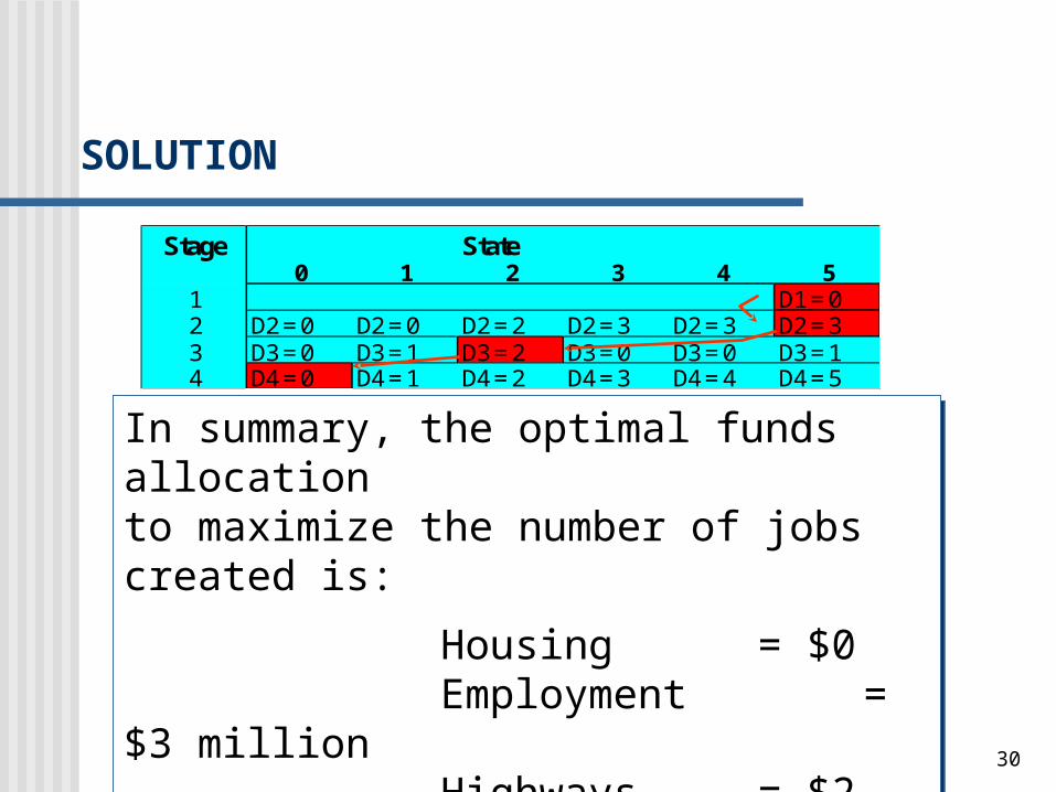
Stage State0 1 2 3 4 5

1 D1 = 02 D2 = 0 D2 = 0 D2 = 2 D2 = 3 D2 = 3 D2 = 33 D3 = 0 D3 = 1 D3 = 2 D3 = 0 D3 = 0 D3 = 14 D4 = 0 D4 = 1 D4 = 2 D4 = 3 D4 = 4 D4 = 5

In summary, the optimal funds allocation to maximize the number of jobs created is:

Housing = $0Employment = $3 millionHighways = $2 millionLaw Enforcement = $0

Maximum number of jobs created = 290

SOLUTION

31

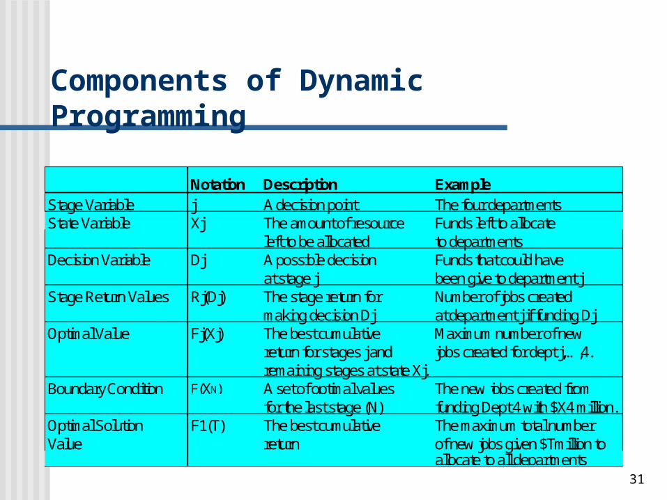
Notation Description ExampleStage Variable j A decision point The four departmentsState Variable Xj The amount of resource Funds left to allocate

left to be allocated to departmentsDecision Variable Dj A possible decision Funds that could have

at stage j been give to department jStage Return Values Rj(Dj) The stage return for Number of jobs created

making decision Dj at department j if funding DjOptimal Value Fj(Xj) The best cumulative Maximum number of new

return for stages j and jobs created for dept j,…,4.remaining stages at state Xj.

Boundary Condition F(XN) A set of optimal values The new jobs created fromfor the last stage (N) funding Dept 4 with $X4 million.

Optimal Solution F1(T) The best cumulative The maximum total number Value return of new jobs given $Tmillion to

allocate to all departments

Components of Dynamic Programming

32

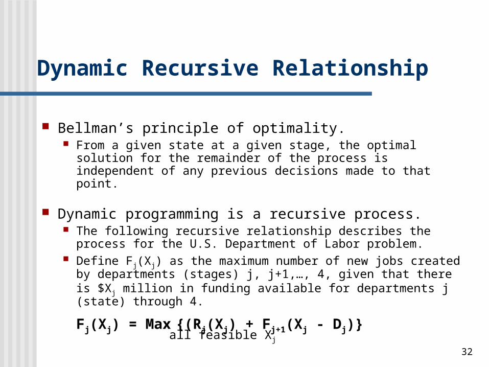
Bellman’s principle of optimality. From a given state at a given stage, the optimal solution for the

remainder of the process is independent of any previous decisions made to that point.

Dynamic programming is a recursive process. The following recursive relationship describes the process for the

U.S. Department of Labor problem. Define Fj(Xj) as the maximum number of new jobs created by

departments (stages) j, j+1,…, 4, given that there is $Xj million in funding available for departments j (state) through 4.

Fj(Xj) = Max {(Rj(Xj) + Fj+1(Xj - Dj)} all feasible Xj

Dynamic Recursive Relationship

33

The form of the recursion relation differs from problem to problem, but the general idea is the same: Do the best you can for the remaining stages with the remaining resources available.

Dynamic Recursive Relationship

34

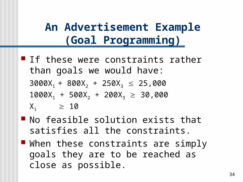
If these were constraints rather than goals we would have:3000X1 + 800X2 + 250X3 25,0001000X1 + 500X2 + 200X3 30,000

X1 10 No feasible solution exists that satisfies all

the constraints. When these constraints are simply goals they

are to be reached as close as possible.

An Advertisement Example(Goal Programming)

35

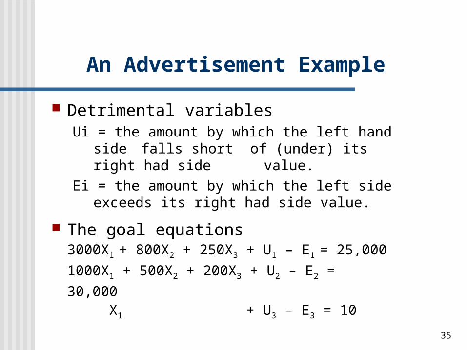
Detrimental variablesUi = the amount by which the left hand side

falls short of (under) its right had side value.

Ei = the amount by which the left side exceeds its right had side value.

The goal equations3000X1 + 800X2 + 250X3 + U1 – E1 = 25,0001000X1 + 500X2 + 200X3 + U2 – E2 = 30,000

X1 + U3 – E3 = 10

An Advertisement Example

36

The objective is to minimize the penalty of not meeting the goals, represented by the detrimental variables

E1, U2, U3.


25,000 30,000 10

37

The penalties are estimated to be as follows:

Each extra dollar spent on advertisement above $25,000 cost the company $1.

There is a loss of $5 to the company for each customer not being reached, below the goal of 30,000.

Each television spot below 10 is worth 100 times each dollar over budget.


38

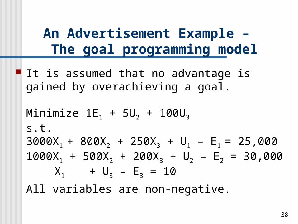
It is assumed that no advantage is gained by overachieving a goal.

Minimize 1E1 + 5U2 + 100U3

s.t.3000X1 + 800X2 + 250X3 + U1 – E1 = 25,0001000X1 + 500X2 + 200X3 + U2 – E2 = 30,000

X1 + U3 – E3 = 10

All variables are non-negative.

An Advertisement Example – The goal programming model

39

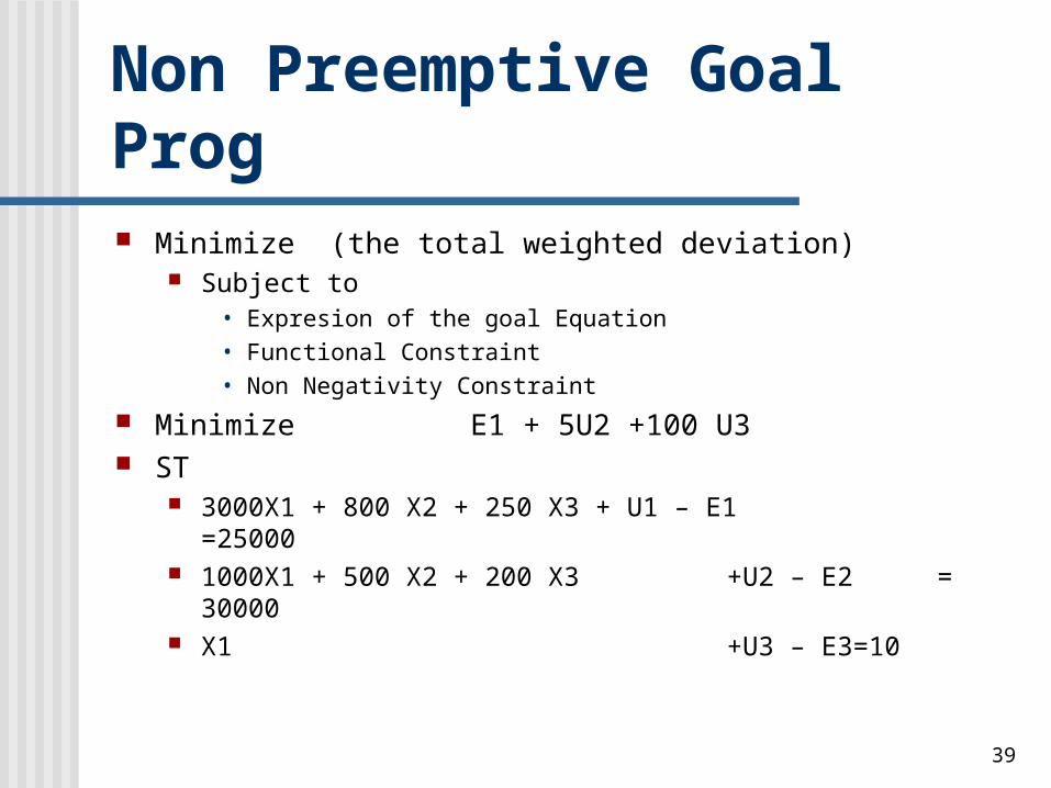
Non Preemptive Goal Prog Minimize (the total weighted deviation)

Subject to • Expresion of the goal Equation• Functional Constraint• Non Negativity Constraint

Minimize E1 + 5U2 +100 U3 ST

3000X1 + 800 X2 + 250 X3 + U1 – E1 =25000 1000X1 + 500 X2 + 200 X3 +U2 – E2 =

30000 X1 +U3 – E3=10

40

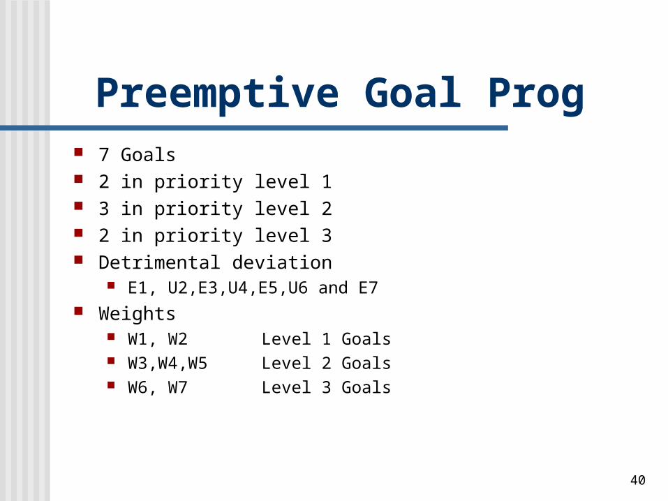
Preemptive Goal Prog 7 Goals 2 in priority level 1 3 in priority level 2 2 in priority level 3 Detrimental deviation

E1, U2,E3,U4,E5,U6 and E7 Weights

W1, W2 Level 1 Goals W3,W4,W5 Level 2 Goals W6, W7 Level 3 Goals

41

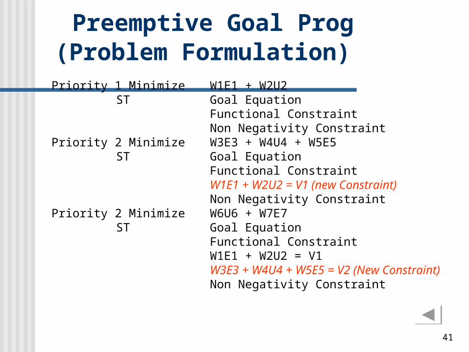
Preemptive Goal Prog(Problem Formulation)

Priority 1 Minimize W1E1 + W2U2ST Goal Equation

Functional ConstraintNon Negativity Constraint

Priority 2 Minimize W3E3 + W4U4 + W5E5ST Goal Equation

Functional ConstraintW1E1 + W2U2 = V1 (new Constraint)Non Negativity Constraint

Priority 2 Minimize W6U6 + W7E7 ST Goal Equation

Functional ConstraintW1E1 + W2U2 = V1 W3E3 + W4U4 + W5E5 = V2 (New Constraint)Non Negativity Constraint

42

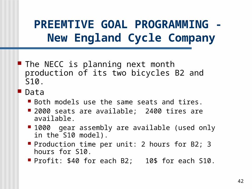
The NECC is planning next month production of its two bicycles B2 and S10.

Data Both models use the same seats and tires. 2000 seats are available; 2400 tires are available. 1000 gear assembly are available (used only in the

S10 model). Production time per unit: 2 hours for B2; 3 hours for

S10. Profit: $40 for each B2; 10$ for each S10.

PREEMTIVE GOAL PROGRAMMING - New England Cycle Company

43

Priority 1: Fulfill a contract for 400 B2 bicycles to be delivered next month.

NECC – Prioritized Goals

Priority 4: At least 200 tires left

over at the end of the month.

At least 100 gear assemblies left over at the end of the month.

Priority 2: Produce at least 1000 total bicycles during the month.

Priority 3: Achieve at least

$100,000 profit for the month.

Use no more than 1600 labor-hours during the month.

44

Management wants to determine the production schedule that best meets its prioritized schedule.

New England Cycle Company Example

45

NECC - SOLUTION Decision variables

X1 = The number of B2s to be produced next month

X2 = The number of S10s to be produced next month Functional / nonnegativity constraints

0X,XTires2400X2X2

assembliesGear1000X

Seats2000XX2

21

21

2

21

46

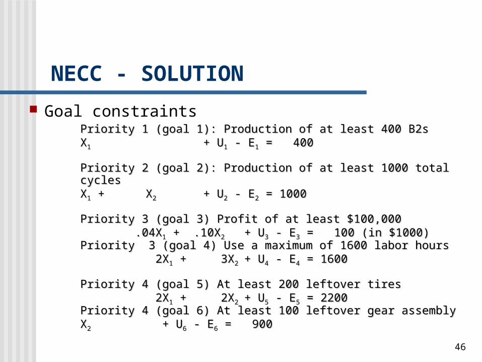
Goal constraints Priority 1 (goal 1): Production of at least 400 B2sPriority 1 (goal 1): Production of at least 400 B2s

XX11 + U+ U11 - E - E11 = 400 = 400

Priority 2 (goal 2): Production of at least 1000 total cyclesPriority 2 (goal 2): Production of at least 1000 total cyclesXX11 + X + X22 + U+ U22 - E - E22 = 1000 = 1000

Priority 3 (goal 3) Profit of at least $100,000Priority 3 (goal 3) Profit of at least $100,000 .04X .04X11 + .10X + .10X22 + U+ U33 - E - E33 = 100 (in $1000) = 100 (in $1000)Priority 3 (goal 4) Use a maximum of 1600 labor hoursPriority 3 (goal 4) Use a maximum of 1600 labor hours 2X 2X11 + 3X + 3X22 + U+ U44 - E - E44 = 1600 = 1600

Priority 4 (goal 5) At least 200 leftover tiresPriority 4 (goal 5) At least 200 leftover tires 2X 2X11 + 2X + 2X22 + U+ U55 - E - E55 = 2200 = 2200Priority 4 (goal 6) At least 100 leftover gear assemblyPriority 4 (goal 6) At least 100 leftover gear assemblyXX22 + U+ U66 - E - E66 = 900 = 900

NECC - SOLUTION

47

Priority level objectives

Priority 1: Underachieving a production of 400 B2s:Minimize U1

Priority 2: Underachieving a total production of 1000: Minimize U2

NECC - SOLUTION

48

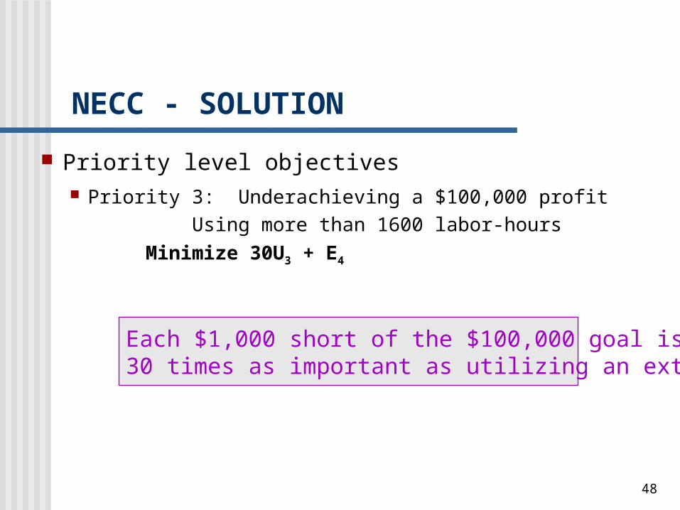
Priority level objectives Priority 3: Underachieving a $100,000 profit Using

more than 1600 labor-hoursMinimize 30U3 + E4

NECC - SOLUTION

Each $1,000 short of the $100,000 goal is considered 30 times as important as utilizing an extra labor-hour.

49

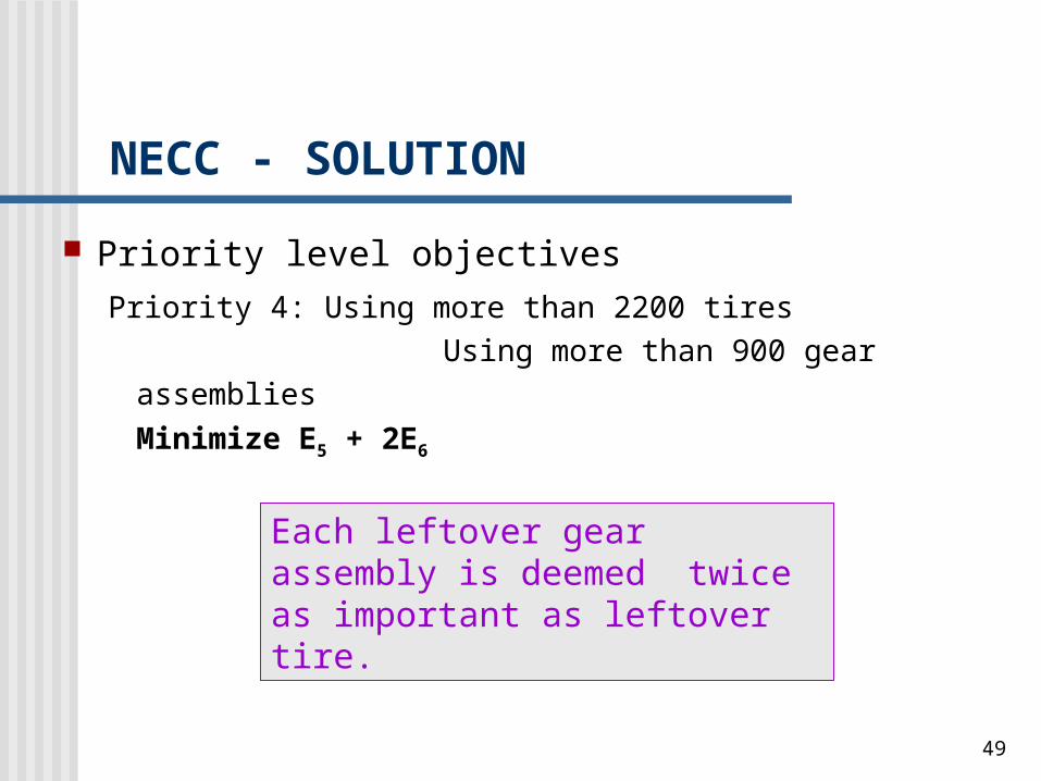
Priority level objectives Priority 4: Using more than 2200 tires

Using more than 900 gear assembliesMinimize E5 + 2E6

NECC - SOLUTION

Each leftover gear assembly is deemed twice as important as leftover tire.

50

Solve the linear goal programming for priority 1 objective, under the set of regular constraints and goal constraint as shown below Minimize U1

ST

NECC - The solution procedure

X1 + U1 - E1 = 400Tires2400X2X2

Gear1000XSeats2000XX2

21

2

21

X1 = 400, thus

U1 = 0, and priority 1 goal is fully achieved.

51

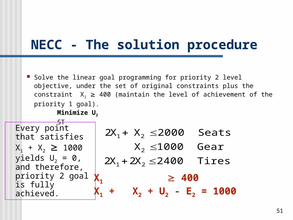
Solve the linear goal programming for priority 2 level objective, under the set of original constraints plus the constraint X1 400 (maintain the level of achievement of the priority 1 goal).

Minimize U2

ST


Every point that satisfies X1 + X2 1000 yields U2 = 0, and therefore, priority 2 goal is fully achieved.

Tires2400X2X2

Gear1000XSeats2000XX2

21

2

21

X1 400X1 + X2 + U2 - E2 = 1000

52

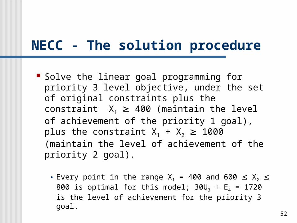
Solve the linear goal programming for priority 3 level objective, under the set of original constraints plus the constraint X1 400 (maintain the level of achievement of the priority 1 goal), plus the constraint X1 + X2 1000 (maintain the level of achievement of the priority 2 goal).

• Every point in the range X1 = 400 and 600 X2 800 is optimal for this model; 30U3 + E4 = 1720 is the level of achievement for the priority 3 goal.


53

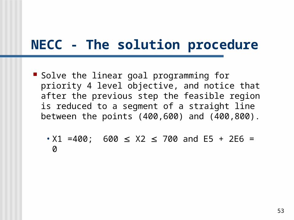
Solve the linear goal programming for priority 4 level objective, and notice that after the previous step the feasible region is reduced to a segment of a straight line between the points (400,600) and (400,800).

• X1 =400; 600 X2 700 and E5 + 2E6 = 0


54

In summary NECC should produce 400 B2 model Between 600 and 700 S10 model

NECC - Solution Summary

55

Unconstraint Models• Single Variable

• Necessary & Sufficient Conditions (df/dx = 0 , D2f/dx2 <> 0))• Multi Variable

• Partial Derivative Constraint Models

• Single Variable• Shadow price• Optimality Criteria

• Multi Variable• Kuhn Tucker Condition

Global View on NLP problems

56

13.7 Unconstrained Nonlinear Programming

One-variable unconstrained problems are demonstrated by the Toshi Camera problem.

The inverse relationships between demand for an item and its value (price) are utilized in this problem.

57

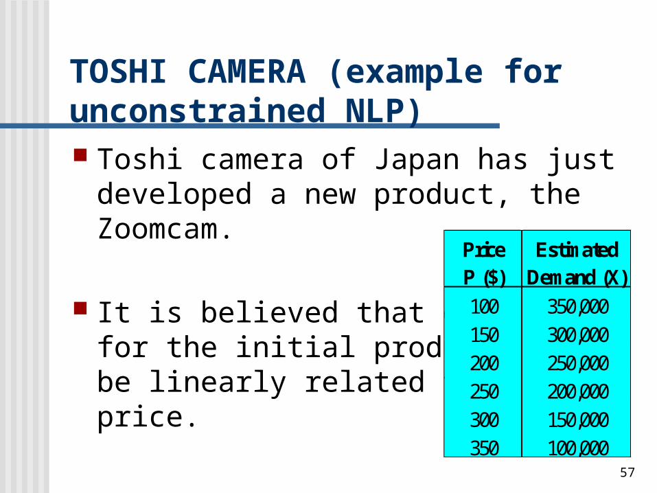
TOSHI CAMERA (example for unconstrained NLP) Toshi camera of Japan has just

developed a new product, the Zoomcam.

It is believed that demand for the initial product will be linearly related to the price.

Price EstimatedP ($) Demand (X)100 350,000150 300,000200 250,000250 200,000300 150,000350 100,000

58

Unit production cost is estimated to be $50. What is the production quantity that

maximizes the total profit from the initial production run?

SOLUTION

Total profit = Revenue - Production cost

F(X) = PX - 50X

TOSHI CAMERA

59

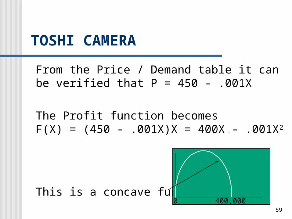
From the Price / Demand table it can be verified that P = 450 - .001X

The Profit function becomesF(X) = (450 - .001X)X = 400X - .001X2

This is a concave function.400,0000

TOSHI CAMERA

60

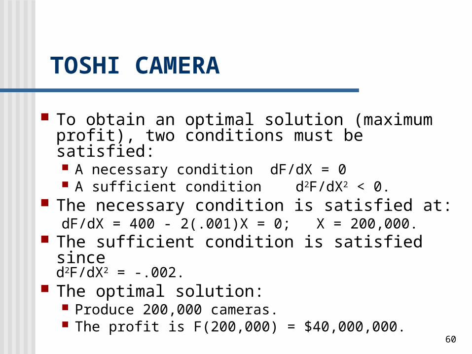
To obtain an optimal solution (maximum profit), two conditions must be satisfied: A necessary condition dF/dX = 0 A sufficient condition d2F/dX2 < 0.

The necessary condition is satisfied at:dF/dX = 400 - 2(.001)X = 0; X = 200,000.

The sufficient condition is satisfied since d2F/dX2 = -.002.

The optimal solution: Produce 200,000 cameras. The profit is F(200,000) = $40,000,000.

TOSHI CAMERA

61

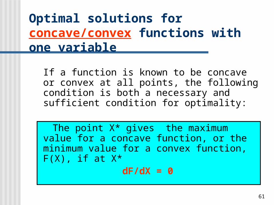
If a function is known to be concave or convex at all points, the following condition is both a necessary and sufficient condition for optimality:

The point X* gives the maximum value for a concave function, or the minimum value for a convex function, F(X), if at X*

dF/dX = 0

Optimal solutions for concave/convex functions with one variable

62

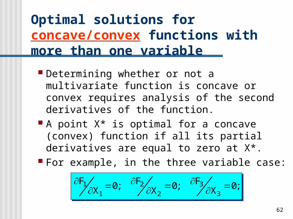
Determining whether or not a multivariate function is concave or convex requires analysis of the second derivatives of the function.

A point X* is optimal for a concave (convex) function if all its partial derivatives are equal to zero at X*.

For example, in the three variable case:

FX

FX

FX

11

22

33

0 0 0 ; ; ;

Optimal solutions for concave/convex functions with more than one variable

63

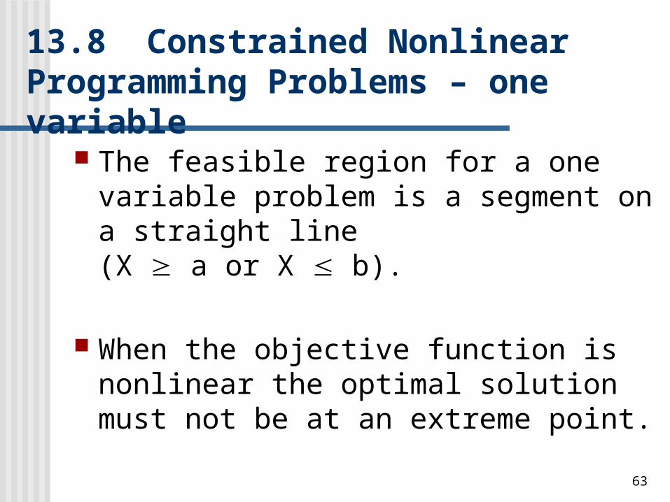
13.8 Constrained Nonlinear Programming Problems – one variable

The feasible region for a one variable problem is a segment on a straight line (X a or X b).

When the objective function is nonlinear the optimal solution must not be at an extreme point.

64

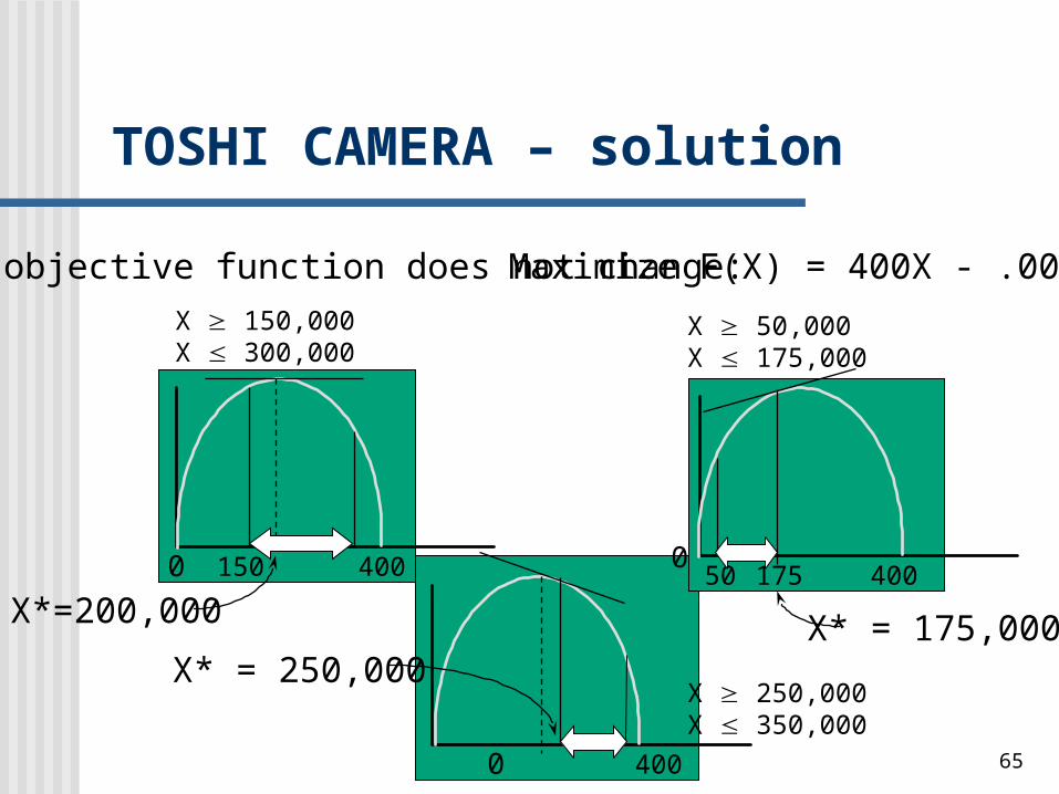
TOSHI CAMERA - revisited

Toshi Camera needs to determine the optimal production level from among the following three alternatives: 150,000 X 300,000 50,000 X 175,000 150,000 X 350,000

654000

X 250,000X 350,000

X* = 250,000

40004000

Maximize F(X) = 400X - .001X2

X 150,000X 300,000

150

X 50,000X 175,000

50 175X*=200,000 X* = 175,000

The objective function does not change:

TOSHI CAMERA – solution

66

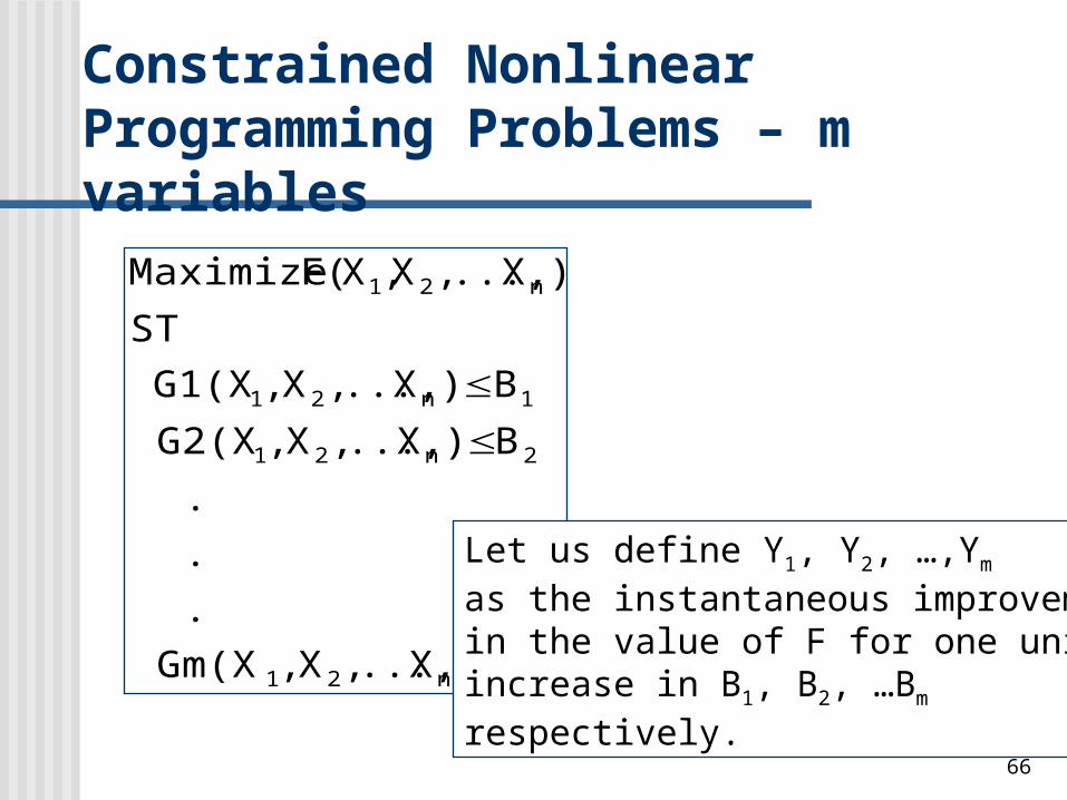
Constrained Nonlinear Programming Problems – m variables

mn21

2n21

1n21

n21

B)X..., ,X ,Gm(X...

B)X..., ,X ,G2(XB)X..., ,X ,G1(X

ST)X..., ,X,X(FMaximize

Let us define Y1, Y2, …,Ym as the instantaneous improvementin the value of F for one unitincrease in B1, B2, …Bm

respectively.

67

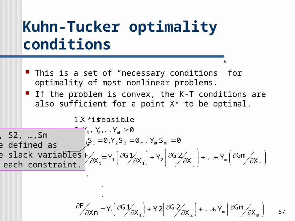
This is a set of “necessary conditions” for optimality of most nonlinear problems.

If the problem is convex, the K-T conditions are also sufficient for a point X* to be optimal.

mm

211

mm2

11

1

mm2211

m21

XGmY...X

2G2YX1GYXn

F

.

..

XGmY...X

2GYX1GYX

F.4

0SY...,,0SY,0SY.30Y..., , Y,Y .2

.feasibleis*X.1

2

S1, S2, …,Smare defined as the slack variablesin each constraint.

Kuhn-Tucker optimality conditions

68

PBI INDUSTRIES

PBI wants to determine an optimal production schedule for its two CD players during the month of April.

Data Unit production cost for the portable CD player = $50.

Unit production cost for the deluxe table player = $90.

There is additional “intermix” cost of $0.01(the number of portable CD’s)(the number of deluxe CD’s).

69

Forecasts indicate that unit selling price for each CD player is related to the number of units sold as follows: Portable CD player unit price = 150 - .01X1 Deluxe CD player unit price = 350 - .02X2

PBI INDUSTRIES

70

Resource usage Each portable CD player uses 1 unit of a particular

electrical component, and .1 labor hour. Each deluxe CD player uses 2 units of the

electrical component, and .3 labor hour. Resource availabilty

10,000 units of the electrical component units; 1,500 labor hours.

PBI INDUSTRIES

71

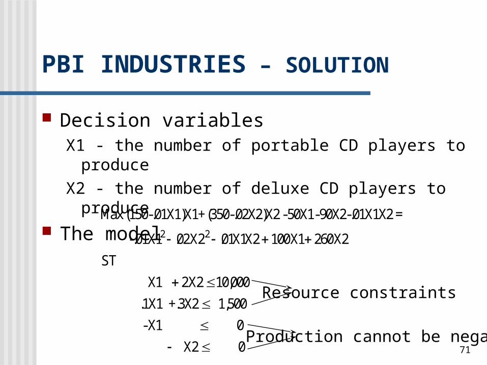
PBI INDUSTRIES – SOLUTION

Decision variablesX1 - the number of portable CD players to produceX2 - the number of deluxe CD players to produce

The modelMax (150-.

X X X X XST

X X

X

01X1)X1+ (350-.02X2)X2 - 50X1- 90X2-.01X1X2 =

-.01X1

.1X1 +.3X2 1,500 - X1

2

. .

,

02 2 01 1 2 100 1 260 2

1 2 2 10 000

02 0

2

Production cannot be negative

Resource constraints

72

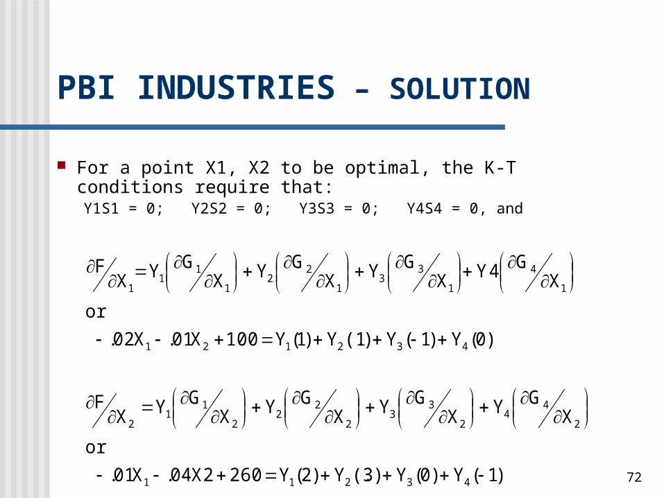
For a point X1, X2 to be optimal, the K-T conditions require that:Y1S1 = 0; Y2S2 = 0; Y3S3 = 0; Y4S4 = 0, and

)1(Y)0(Y)3(.Y)2(Y2602X04.X01.or

XGYX

GYXGYX

GYXF

)0(Y)1(Y)1(.Y)1(Y100X01.X02.or

XG4YX

GYXGYX

GYXF

43211

2

44

2

33

2

22

2

11

2

432121

1

4

1

33

1

22

1

11

1


73

Finding an optimal production plan. Assume X1>0 and X2>0.

• The assumption implies S3>0 and S4>0.• Thus, Y3 = 0 and Y4 = 0.

Add the assumption that S1 = 0 and S2 = 0.• From the first two constraints we have X1 = 0 and

X2 = 5000.X1= 0

A contradictionX1>0

AS A RESULT THE SECOND ASSUMPTION CANNOT BE TRUE


74

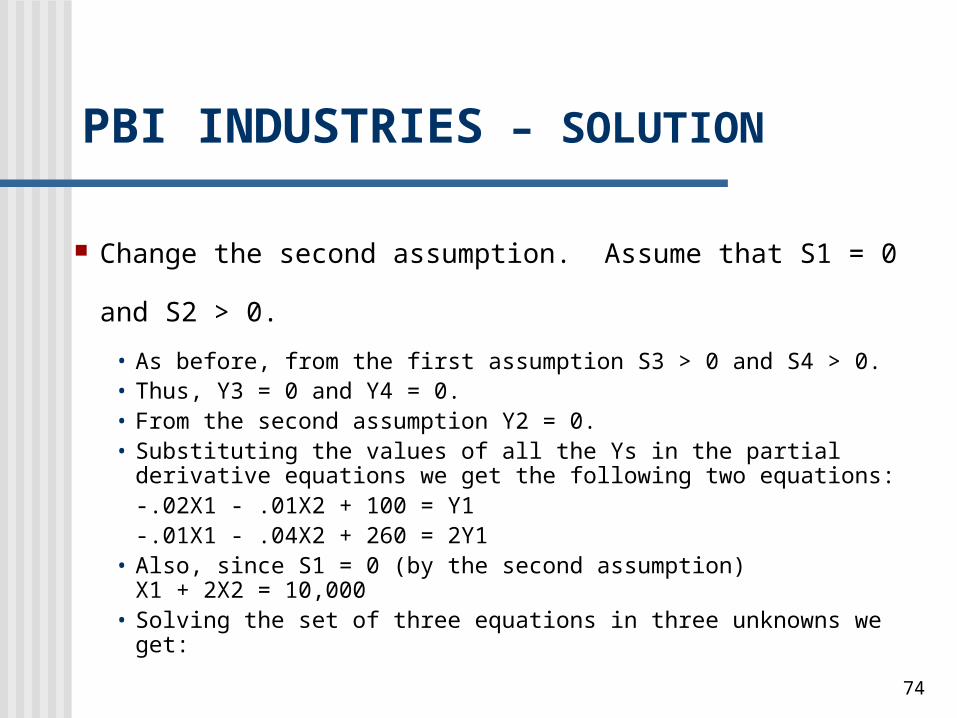
Change the second assumption. Assume that S1 = 0 and S2 > 0.

• As before, from the first assumption S3 > 0 and S4 > 0.• Thus, Y3 = 0 and Y4 = 0.• From the second assumption Y2 = 0.• Substituting the values of all the Ys in the partial derivative

equations we get the following two equations:-.02X1 - .01X2 + 100 = Y1-.01X1 - .04X2 + 260 = 2Y1

• Also, since S1 = 0 (by the second assumption)X1 + 2X2 = 10,000

• Solving the set of three equations in three unknowns we get:


75

X1 = 1000, X2 = 4500, Y1 = 35 This solution is a feasible point (check the constraints).

• X1 and X2 are positive.• 1X1 + 2X2 <= 10,000 [1000 + 2(4500) = 10,000]• .1X1 + .3X2 <= 1,500 [.1(1000) + .3(4500) = 1450]

This problem represents a convex program since• It can be shown that the objective function F is concave.• All the constraints are linear, thus, form a convex set.

The K-T conditions yielded an optimal solution


76

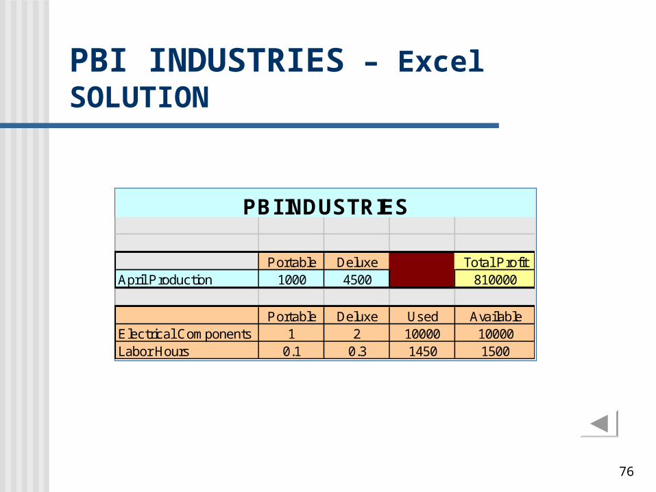
Portable Deluxe Total ProfitApril Production 1000 4500 810000

Portable Deluxe Used AvailableElectrical Components 1 2 10000 10000Labor Hours 0.1 0.3 1450 1500

PBI INDUSTRIES

PBI INDUSTRIES – Excel SOLUTION

Ch13 - NLP,DP,GP2005

Documents

Transcript of Ch13 - NLP,DP,GP2005