Cfx12 04 solver

4-1ANSYS, Inc. Proprietary© 2009 ANSYS, Inc. All rights reserved.

April 28, 2009Inventory #002598

Chapter 4

Solver Settings

Introduction to CFX

Solver Settings



Training ManualOverview

• Initialization

• Solver Control

• Output Control

• Solver Manager

Note: This chapter considers solver settings for steady-state simulations. Settings specific to transient simulation are discussed in a later chapter.

Solver Settings



Training Manual

• Iterative solution procedures require that all solution variables are assigned initial values before calculating a solution

• A good initial guess can reduce the solution time

• In some cases a poor initial guess may cause the solver to fail during the first few iterations

• The initial values can be set in 3 ways:

1. Solver automatically calculates the initial values

2. Initial values are entered by the user

3. Initial values are obtained from a previous solution

• Initial values can be set on a per-domain basis or globally for all domains

Initialization

Solver Settings



Training ManualInitialization – Setting Initial Values

• Insert Global Initialisation from the toolbar or by right-clicking on Flow Analysis 1

• Edit each Domain to set initial values on a per-domain basis– When both are defined the

domain settings take precedence

– Solid domain must have initial conditions set on a per-domain basis

Solver Settings



Training ManualInitialization – Setting Initial Values

• The Automatic option means that the CFX-Solver will calculate an initial value for the solved variable unless a previous results file is provided– Will be based on boundary condition

values and domain settings

• The Automatic with Value option means that the specified value will be used unless a previous results file is provided– Can use a constant value or an expression

Solver Settings



Training ManualInitialization – Using a Previous Solution

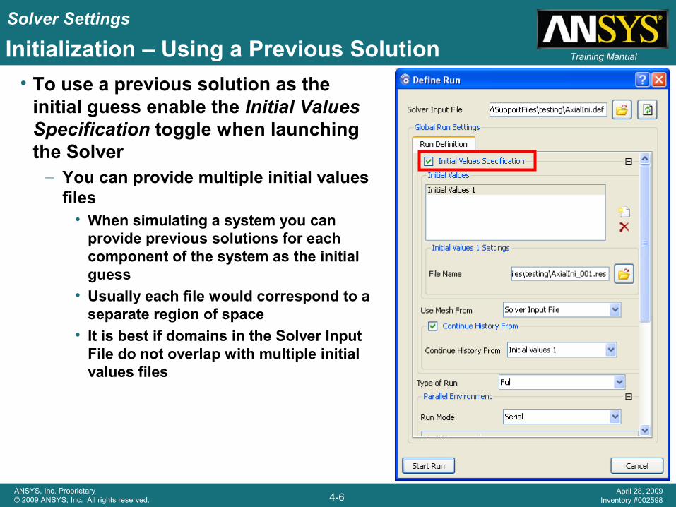
• To use a previous solution as the initial guess enable the Initial Values Specification toggle when launching the Solver– You can provide multiple initial values

files• When simulating a system you can

provide previous solutions for each component of the system as the initial guess

• Usually each file would correspond to a separate region of space

• It is best if domains in the Solver Input File do not overlap with multiple initial values files

Solver Settings



Training Manual

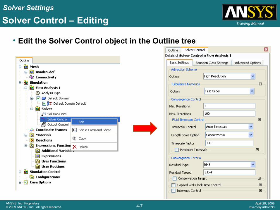
• Edit the Solver Control object in the Outline tree

Solver Control – Editing

Solver Settings



Training Manual

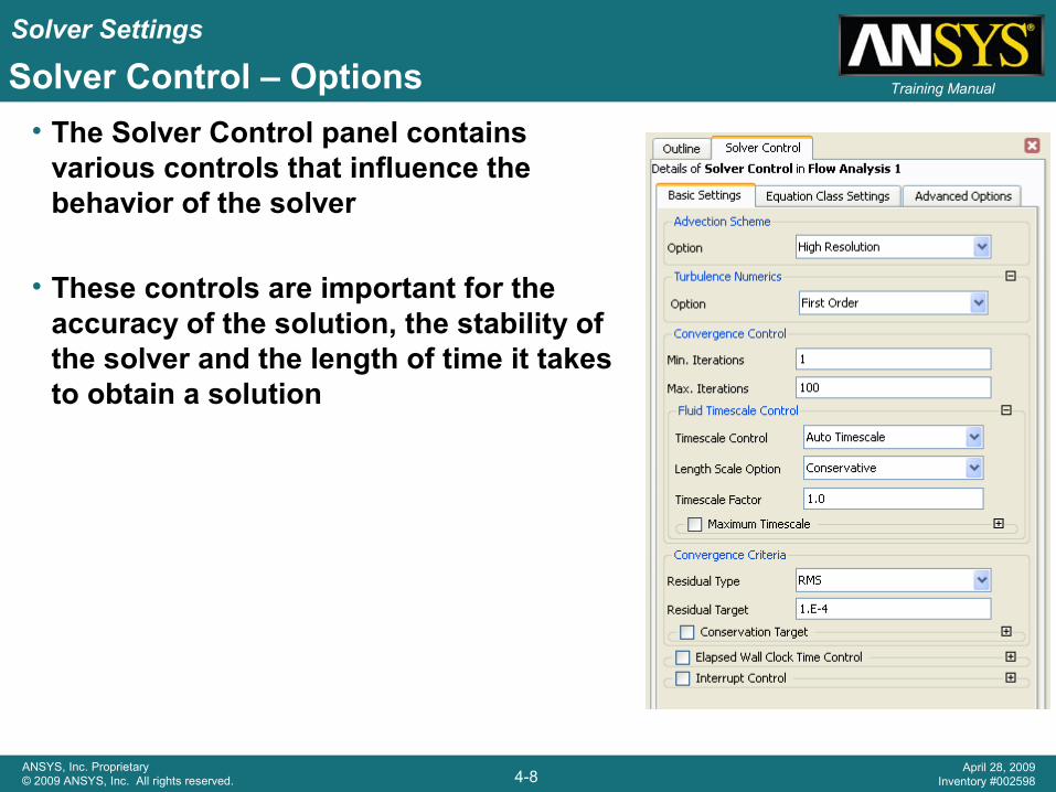
• The Solver Control panel contains various controls that influence the behavior of the solver

• These controls are important for the accuracy of the solution, the stability of the solver and the length of time it takes to obtain a solution

Solver Control – Options

Solver Settings



Training ManualSolver Control – Advection Scheme

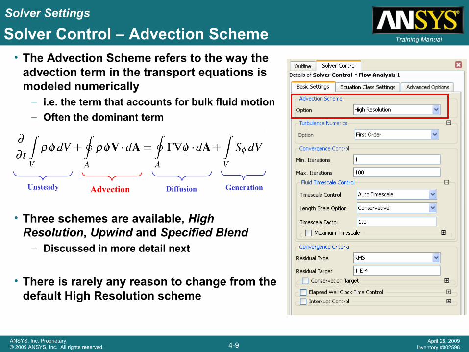
• The Advection Scheme refers to the way the advection term in the transport equations is modeled numerically– i.e. the term that accounts for bulk fluid motion– Often the dominant term

• Three schemes are available, High Resolution, Upwind and Specified Blend– Discussed in more detail next

• There is rarely any reason to change from the default High Resolution scheme

Unsteady Advection Diffusion Generation

Solver Settings



Training ManualSolver Control – Advection Scheme Theory

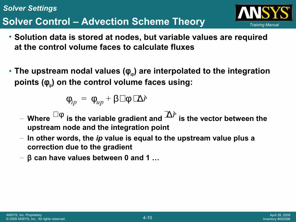
• Solution data is stored at nodes, but variable values are required at the control volume faces to calculate fluxes

• The upstream nodal values (φ up) are interpolated to the integration points (φ ip) on the control volume faces using:

– Where is the variable gradient and is the vector between the upstream node and the integration point

– In other words, the ip value is equal to the upstream value plus a correction due to the gradient

– β can have values between 0 and 1 …

φip φup β φ∇ ∆r⋅+=

∇φ φip φup β φ∇ ∆r⋅+=

Solver Settings



Training ManualSolver Control – Advection Scheme Theory

• If β = 0 we get the Upwind advection scheme, i.e. no correction– This is robust but only first order accurate– Sometimes useful for initial runs, but

usually not necessary

• The Specified Blend scheme allows you to specify β between 0 and 1 (i.e. between no correction up to full correction)– But this is not guaranteed to be bounded,

meaning that when the correction is included it can overshoot or undershoot what is physically possible

• The High Resolution scheme maximizes β throughout the flow domain while keeping the solution bounded

φip φup β φ∇ ∆r⋅+= Theory

High ResolutionScheme

Upwind Scheme

β=1.00

Flow is misaligned with mesh

0

1

Solver Settings



Training ManualSolver Control – Turbulence Numerics

• Regardless of the Advection Scheme selection, the Turbulence equations default to the First Order (Upwind) scheme– Usually this is sufficient

• The High Resolution scheme can be selected for additional accuracy– Can give better accuracy in boundary

layers on unstructured meshes

Solver Settings



Training ManualSolver Control – Convergence Control

• The Solver will finish when it reaches Max. Iterations unless convergence is achieved sooner– If Max. Iterations is reached you may not have

a converged solution– Can be useful to set Max. Iterations to a large

number

• When the Solver finishes you should always check why it finished

• Fluid Timescale Control sets the timescale in a steady-state simulation …

Solver Settings



Training Manual

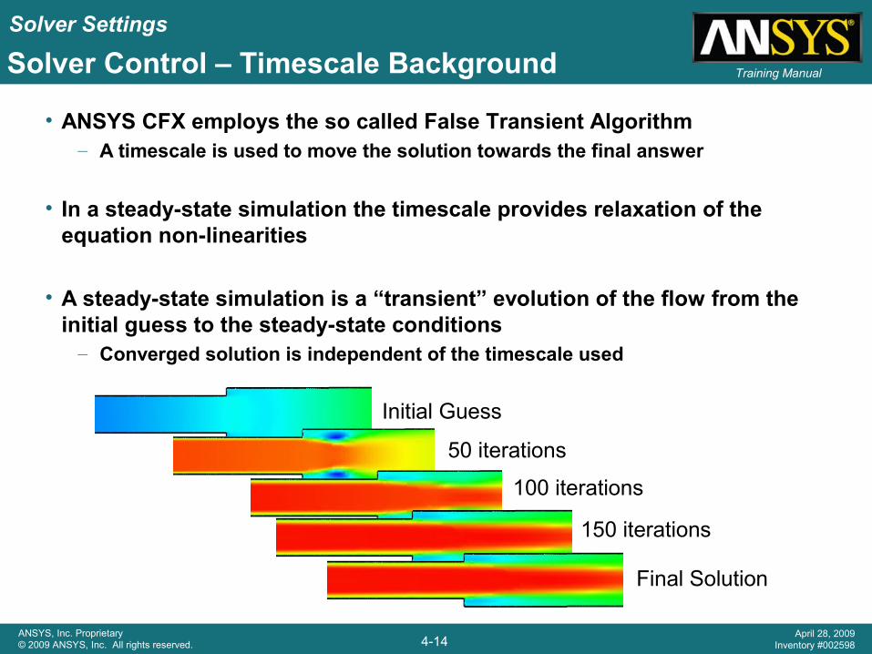
• ANSYS CFX employs the so called False Transient Algorithm– A timescale is used to move the solution towards the final answer

• In a steady-state simulation the timescale provides relaxation of the equation non-linearities

• A steady-state simulation is a “transient” evolution of the flow from the initial guess to the steady-state conditions– Converged solution is independent of the timescale used

Initial Guess

50 iterations

100 iterations

150 iterations

Final Solution

Solver Control – Timescale Background

Solver Settings



Training Manual

• For obtaining successful convergence, the selection of the timescale plays an important role

– If the timescale is too large, the convergence becomes bouncy or may even lead to the failure of the Solver

– If the timescale is too small, the convergence will be very slow and the solution may not be fully accurate

Solver Control – Timescale Selection

Solver Settings



Training ManualSolver Control – Timescale Selection

• For advection dominated flow, a fraction of the fluid residence time is often a good estimate for the timescale– A timescale of 1/3 of (Length Scale / Velocity Scale) is often optimal

– May need a smaller timescale for the first few iterations and for complex physics, transonic flow,…..

• For rotating machines, 1/ω (ω in rad/s) is a good choice

• For buoyancy driven flows, the timescale should be based on a function of gravity, thermal expansivity, temperature difference and length scale (see documentation)

Solver Settings



Training Manual

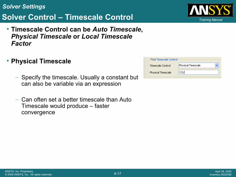
• Timescale Control can be Auto Timescale, Physical Timescale or Local Timescale Factor

• Physical Timescale

– Specify the timescale. Usually a constant but can also be variable via an expression

– Can often set a better timescale than Auto Timescale would produce – faster convergence

Solver Control – Timescale Control

Solver Settings



Training ManualSolver Control – Timescale Control

• Auto Timescale– The Solver calculates a timescale based on

boundary / initial conditions or current solution and domain length scale

– Use a Conservative or Aggressive estimate for the domain length scale, or a specified value

– Timescale is re-calculated and updated every few iterations as the flow field changes

– Can set a Maximum Timescale to provide an upper limit

– Tends to produce a conservative timescale

– Timescale factor (default = 1) is a multiplier which can be changed to adjust the automatically calculated timescale

Solver Settings



Training Manual

• Local Timescale Factor– Timescale varies throughout the domain

– Can accelerate convergence when vastly different local velocity scales exist• E.g. a jet entering a plenum

– Best used on fairly uniform meshes, since small element will have a small timescale which can slow convergence

– Local Timescale Factor is a multiplier of the local timescale– Never use as final solution; always finish off with a constant timescale

Local Timescale =Local Mesh Length Scale

Local Velocity Scale

Smaller Timescale in high velocity and/or fine mesh regions

Solver Control – Timescale Control

Solver Settings



Training ManualSolver Control – Convergence Criteria

• Convergence Criteria settings determine when the solution is considered converged and hence when the Solver will stop– Assuming Max. Iterations is not reached

• Residuals are a measure of how accurately the set of equations have been solved– Since we are iterating towards a solution, we never

get the exact solution to the equations– Lower residuals mean a more accurate solution to

the set of equations (more on the next slide)– Do not confuse accurately solving the equations

with overall solution accuracy – the equations may or may not be a good representation of the true system!

– Residuals are just one measure of accuracy and should be combined with other measures:

• Monitor Points (ch. 8) and Imbalances (below)

Solver Settings



Training Manual

• The continuous governing equations are discretized into a set of linear equations that can be solved. The set of linear equations can be written in the form:

[A] [Φ] = [b]

where [A] is the coefficient matrix and [Φ] is the solution variable

• If the equation were solved exactly we would have:

[A] [Φ] - [b] = [0]

• The residual vector [R] is the error in the numerical solution:

[A] [Φ] - [b] = [R]

• Since each control volume has a residual we usually look at the RMS average or the maximum normalized residual

Solver Control – Residuals Theory

Solver Settings



Training Manual

• Residual Type– MAX: Convergence based on maximum

residual anywhere– RMS: Convergence based on average

residual from all control volumes

– Root Mean Square =

• Residual Target– For reasonable convergence MAX residuals

should be 1.0E-3, RMS should be at least 1.0E-4

– The targets dependent on the accuracy needed

• Lower values may be needed for greater accuracy

n

2∑i

iR

Solver Control – Residuals

Solver Settings



Training ManualSolver Control – Conservation Target• The Conservation Target sets a target for the

global imbalances

• The imbalances measure the overall conservation of a quantity (mass, momentum, energy) in the entire flow domain

Flux Maximum

OutFlux InFlux Imbalance %

−=

• Clearly in a converged solution Flux In should equal Flux Out

• It’s good practice to set a Conservation Target and/or monitor the imbalances during the run

• When set, the Solver must meet both the Residual and Conservation Target before stopping (assuming Max. Iterations is not reached)

• Set a target of 0.01 (1%) or less– Flux In – Flux Out < 1%

Solver Settings



Training Manual

• Elapsed Time Control– Can specify the maximum wall clock time

for a run– Solver will stop after this amount of time

regardless of whether it has converged

• Interrupt Control– Can specify other criteria for stopping

the Solver based on logical CEL expressions

– When the expression returns true the solver will stop

• Any value >= 0.5 is true

Solver Control – Elapsed Time and Interrupt Control

– Examples• If temperature exceeds a specified value

if(areaAve(T)@wall>200[C],1,0)

• If mesh quality drops below a specified value in a moving mesh case

– More on logical expressions in the CEL lecture

Solver Settings



Training Manual

• This option is only available when a solid domain is included in the simulation

• The Solid Timescale should be selected such that it is MUCH larger than the fluid timescale (100 times larger is typical)

– the energy equation is usually very stable in the solid zone

– solid timescales are typically much larger than fluid timescales

Solver Control – Solid Timescale Control

• The fluid timescale is estimated using Length Scale / Velocity Scale

• The solid timescale is automatically calculated as function of the length scale, thermal conductivity, density and specific heat capacity

– Or you can choose the Physical Timescale option and provide a timescale directly

Solver Settings



Training Manual

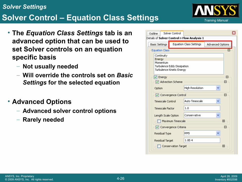
• The Equation Class Settings tab is an advanced option that can be used to set Solver controls on an equation specific basis

– Not usually needed– Will override the controls set on Basic

Settings for the selected equation

• Advanced Options– Advanced solver control options– Rarely needed

Solver Control – Equation Class Settings

Solver Settings



Training ManualOutput Controls – Results

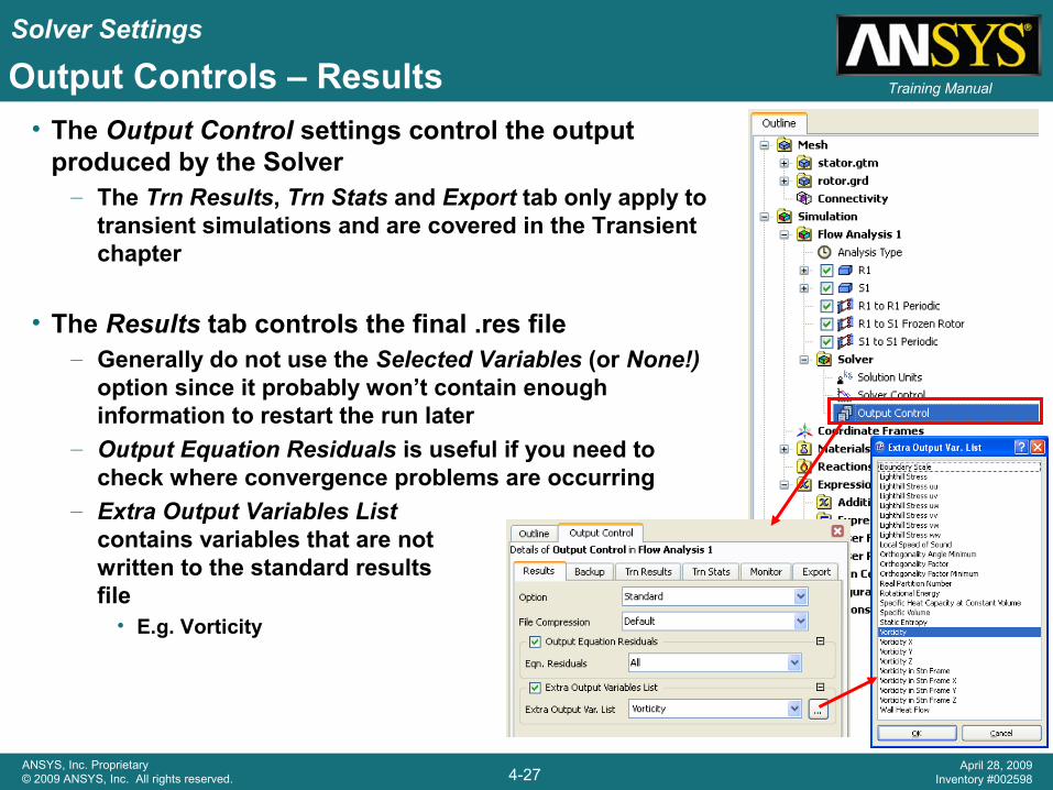
• The Output Control settings control the output produced by the Solver

– The Trn Results, Trn Stats and Export tab only apply to transient simulations and are covered in the Transient chapter

• The Results tab controls the final .res file– Generally do not use the Selected Variables (or None!)

option since it probably won’t contain enough information to restart the run later

– Output Equation Residuals is useful if you need to check where convergence problems are occurring

– Extra Output Variables Listcontains variables that are notwritten to the standard resultsfile

• E.g. Vorticity

Solver Settings



Training Manual

Frequency of output can be adjusted

Output Controls – Backup

• The Backup tab controls if and when backup results files are automatically written by the Solver

• Recommend for long Solver runs in case of power failure, network interruptions, etc

• Option:– Standard: Like a full results file– Essential: Allows a clean solver restart– Smallest: Can restart the solver, but there’ll

be a jump in the residuals– Selected Variables: Not recommended

• Can also manually request a backup file from the Solver Manager at any time

Solver Settings



Training Manual

• The Monitor tab allows you to create Monitor Points

– These are used to track values of interest as the Solver runs

• The Cartesian Coordinates Option is used to track the value of a variable at a specific X, Y, Z location

• The Expression Option is used to monitor the values of a CEL expression

– E.g. Calculate the area average of Cp at the inlet boundary: areaAve(Cp)@inlet

– E.g. Mass flow of particular fluid through an outlet: oil.massFlow()@outlet

• In steady-state simulations you should create monitor points for quantities of interest

– One measure of convergence is when these values are no longer changing

Output Controls – Monitor

Solver Settings



Training Manual

• The CFX-Solver Manager is a graphical user interface used to:– Define a run– Control the CFX-Solver interactively– View information about the emerging solution– Export data

Solver Manager

Solver Settings



Training Manual

• Define a new Solver run

• Solver Input File should be the .def file– Can also pick .res, .bak or _full.trn files to restart a

previous incomplete run

• To make a physics change and restart a solution, create a new .def file and provide it as the Solver Input File then select the .res, .bak or _full.trn file in the Initial Values Specification section– If both files have the same physics, this is the same

as picking the .res/.bak/_full.trn file as the input file

• Use Mesh From selects which mesh to use. If the meshes are identical can use either option, otherwise:– If you use the Solver Input File mesh, the Initial

Values solution is interpolated onto the input file– If you use the Initial Values mesh only the physics

from the Solver Input File is used

• Continue History From carriers over convergence history and iteration counters

Solver Manager – Defining a Run

Solver Settings



Training ManualSolver Manager – Defining a Parallel Run

• By default the Solver will run in serial– A single solver process runs on the local

machine

• Set the Run Mode to one of the parallel options to make use of multiple cores/processors– Requires parallel licenses– Allows you to divide a large CFD problem into

smaller partitions• Faster solution times• Solve larger problems by making use of memory

(RAM) on multiple machines

• The Local Parallel options should be used when running on a single machine

• The Distributed Parallel options should be used when running across multiple machines

Solver Settings



Training Manual

• Serial

• Local Parallel

• Distributed Parallel

• Different communication methods are available (MPICH2, HP MPI, PVM)– See documentation “When To Use MPI or PVM” for more details, but HP MPI is

recommended in most cases

Solver Manager – Defining a Parallel Run

Solver Settings



Training Manual

• The Show Advanced Control toggle enables the Partitioner, Solver and Interpolator tabs

• On the Partitioner tab you can pick different partitioning algorithms– Partitioning is always a serial process– Can be a problem for v.large cases since you

cannot distribute the memory load across multiple machines

– The default MeTiS algorithm uses more memory than others, so if you run out of memory use a different method (see documentation for details)

• Multidomain Option:– Independent Partitioning: Each domain is

partitioned into n partitions– Coupled Partitioning: All domains are combined

and then partitioned into n partitions• There’s a specific option for Transient Rotor Stator

cases

Solver Manager – Define Run Advanced Controls

Solver Settings



Training Manual

• On the Solver tab you can select the Double Precision option– The solver will use more significant figures in its

calculations– Doubles solver memory requirements– Use when round-off error could be a problem – if

‘small’ variations in a variable are important, where ‘small’ is relative to the global range of that variable, e.g:

• Many Mesh Motion cases, since the motion is often small relative to the size of the domain

• Most CHT cases, since thermal conductivity is vastly different in the fluid and solid

• If you have a wide pressure range, but small pressure changes are important

– Small values by themselves do not need DP

Solver Manager – Define Run Advanced Controls

• The Solver estimates its memory requirements upfront• Memory Alloc Factor is a multiplier for this estimate

– Use when the solver stops with an “Insufficient Memory Allocated” error

Solver Settings



Training ManualSolver Manager – Interactive Solver Control

• During a solution Edit Run in Progress lets you make changes on the fly– Models generally cannot be changed, but timescales, BC’s, etc can

Solver Settings



Training Manual

.out fileMonitor Plot

Solver Manager – Additional Solution Monitors

Right-click

• By default monitor plots are created showing the RMS residuals for each equation solved, plus one plot for any monitor points

• Right-click to switch between RMS and MAX

• Additional monitors can be selected showing:– Imbalances– Boundary fluxes (FLOW)– Boundary forces

• Tangential (viscous)• Normal (pressure)

– Source terms …

New Monitor

Solver Settings



Training Manual

Start a new Simulation

Monitor Run in Progress

Monitor Finished Run

Stop Current Run

Save Current Run

Switch Residual Plot

between RMS and

MAX

• By dragging the cursor over any icon, the feature description will appear

Solver Manager – Additional Icons

Cfx12 04 solver

Documents

Transcript of Cfx12 04 solver