i

B. Tech Thesis on

CFD Simulation of Pressure Drop and Liquid Holdup

in a Trickle Bed Reactor

For partial fulfilment of the requirement for the degree of

Bachelor of Technology

In

Chemical Engineering

Submitted by: Antariksha Pattnaik

Roll No. 111CH0600

Under the supervision of:

Prof (Dr.) H. M. Jena

Department of Chemical Engineering,

National Institute of Technology, Rourkela

2015

ii

National Institute of Technology, Rourkela

CERTIFICATE

This is to certify that the thesis entitled “CFD Simulation of Pressure drop and liquid holdup in a

Trickle Bed Reactor” submitted by Antariksha Pattnaik, Roll No.-111CH0600, in partial fulfilment

of the requirement for the award of degree of Bachelor of Technology in Chemical Engineering at

National Institute of Technology Rourkela, is an authentic work carried out by him under my

supervision and guidance.

Date: Prof. (Dr.) H. M. Jena

Place: Rourkela Department of Chemical Engineering

National Institute of Technology, Rourkela-769008

iii

ACKNOWLEDGEMENT

I would like to express my deepest gratitude to Prof (Dr.) H. M. Jena for his valuable guidance and

encouragement during every stage of the project. I am very thankful to him for providing me the right

guidance to work on an emerging area of chemical engineering. He was very supportive throughout

the project and was always ready to help.

I am also grateful to Prof P. Rath, Head of the Department, Chemical Engineering for providing the

necessary facilities for the completion of this project.

I would like to thanks all my faculties and friends of Chemical Engineering Department, NIT

Rourkela for their support and encouragement. Lastly I would like to thanks my parents for their

constant support, encouragement and well wishes, without which this thesis wouldn’t have been

possible.

Antariksha Pattnaik

Roll No-111CH0600

Department of Chemical Engineering

NIT Rourkela.

iv

ABSTRACT

Trickle Bed Reactors have etched a ubiquitous presence in chemical processing sector. From

petroleum and petrochemical products, fine chemicals to biochemical, wastewater treatment, they are

almost everywhere. Products worth of 300 billion US $ are processed by these reactors on an annual

average. A complete understanding of hydrodynamics, fluid phase mixing, interphase and

interparticle heat and mass transfer and reaction kinetics of TBR can help us to extract the full

potential of TBR. Studying the variation of pressure drop and liquid holdup is crucial for evaluation

of performance of trickle bed reactors and can help in further optimizing their performance.

This project focuses on the effect of gas and liquid velocities on the pressure drop and liquid holdup

in a trickle-Bed reactor operating at ambient temperature and atmospheric pressure. Pressure drop

and liquid holdup are two critical hydrodynamics parameters that influence other parameters directly

and indirectly and hence, these two parameters are preferred for hydrodynamic study of TBR. Their

variation along longitudinal and transverse direction is the focus of this project. A comparison of

results from different simulation scenarios (using different pressure values as patching values) made

in this project helps in understanding how different initial guess can affect the final solution in

simulating real-life TBR operation. It is found that pressure ranging up to 10000 Pa as patching

pressure value can lead to a converging solution. Afterwards, solution instability creeps in leading to

impractically higher values of pressure and liquid holdup and sometimes ending up with divergence.

Even the effect of gas and liquid velocity is studied on the two parameters. The variation of the two

hydrodynamic parameters with changing liquid velocities and gas velocities are also studied.

Keywords: TBR, Hydrodynamics, Pressure drop, Liquid holdup

v

CONTENTS

Title Page i

Certificate ii

Acknowledgement iii

Abstract iv

Contents v

List of Figures vii

List of Tables viii

List of Symbols used ix

Abbreviations x

Chapter 1 Introduction 1-6

1.1 Definition 1

1.2 Configurations of Trickle Bed Reactors 1

1.3 Flow Regimes 2

1.4 Performance Indicators of Trickle Bed Reactor 3

1.5 Advantages and Disadvantages of Trickle Bed Reactor 4

1.6 Applications of Trickle Bed Reactor 5

1.7 Objective and Scope of the Work 5

Chapter 2 Literature Review 6-8

2.1 Computational studies on Trickle Bed Reactor 6

2.2 Drag Force Models used in CFD 6

2.2.1 Empirical/phenomenological models 6

2.2.2 Semi-empirical models 7

2.2.2.1 Relative Permeability model 7

2.2.2.2 Slit Model 7

2.2.2.3 Fluid-Fluid Interaction Model 7

Chapter 3 CFD Modeling 9-14

3.1 Definition of CFD 8

3.2 Basic Governing Equations 8

3.3 Basic Fluid Flow Models 9

vi

3.3.1 Euler-Lagrangian approach 9

3.3.2 Euler-Euler approach 10

3.3.2.1 Volume of Fluid Model 10

3.3.2.2 Mixture Model 10

3.3.2.3 Eulerian Model 11

3.4 Drag Force Calculation 11

3.5 Turbulence Model (k-ε model) 11

3.6 Porous Media Model 12

Chapter 4 FLUENT Simulation Work 14-17

4.1 Geometry and mesh 14

4.2 Assumptions 15

4.3 Boundary conditions and Numerical Solutions 15

Chapter 5 Results and discussion 17-21

5.1 Transverse and longitudinal variation of pressure and liquid holdup 17

5.2 Effect of patching with different pressure on the solution 18

5.3 Different gas and liquid velocities 19

CONCLUSION 22

REFERENCES 23

vii

LIST OF FIGURES

Figure No. Caption Page No.

Figure 1.1 Various configurations of Trickle Bed Reactors (Ranade et al.) 1

Figure1.2 Flow Regime in gas-liquid contact (Gunjal et al. 2005) 3

Figure 3.1 Various Linear Eddy Viscosity Models 13

Figure 4.1 Structured grid for simulation 14

Figure 4.2 Lines on geometry 16

Figure 5.1 Scaled Residual plot showing convergence 17

Figure 5.2 Axial variation of Pressure drop 18

Figure 5.3 Axial variation of Liquid holdup 18

Figure 5.4 Radial variation of Liquid holdup 18

Figure 5.5 Axial variation of Pressure drop for different pressure patching 19

Figure 5.6 Axial variation of liquid holdup for different pressure patching 19

Figure 5.7 Radial variation of Liquid holdup for different pressure patching 19

Figure 5.8 Axial variation of Pressure variation at different liquid velocity and

Ug=0.22 m/s

20

Figure 5.9 Axial variation of Pressure variation at different liquid velocity and

Ug=0.33 m/s

20

Figure 5.10 Axial variation of liquid holdup at different liquid velocity and

Ug=0.22 m/s

21

Figure 5.11 Axial variation of liquid holdup at different liquid velocity and

Ug=0.22 m/s

21

Figure 5.12 Axial variation of liquid holdup at different liquid velocity and

Ug=0.22 m/s

21

Figure 5.13 Axial variation of liquid holdup at different liquid velocity and

Ug=0.22 m/s

21

viii

LIST OF TABLES

Table Caption Page No.

Table 1.1 Industrial Applications of Trickle Bed Reactors 5

Table 4.1 Geometry specification of TBR 14

Table 4.2 Mesh report 15

Table 4.3 Operating conditions and models used 15

Table 4.4 Solutions settings 16

ix

LIST OF SYMBOLS USED

α permeability of porous media, m2

αk volume fraction of k phase

C0, C1 user-defined empirical constants for power law form of Darcy’s Law

C2 internal resistance factor, 1/m

∇. divergence (gradient operator with dot product)

dp effective particle diameter, m

ε turbulence dissipation rate, J/kg; bed voidage

Ek energy for phase k, J

F body force, N

g acceleration due to gravity, m/s2

hk sensible enthalpy for phase k, J/mole

k kinetic energy, J

keff effective thermal conductivity, W/(m.K)

kt turbulent conductivity, W/(m.K)

µk viscosity of k phase, kg/(m.s)

µm viscosity of mixture, kg/(m.s)

P pressure, Pa

density of phase k, kg/m3

ρm mixture density, kg/m3

SE any other volumetric heat source, W/m2

Si momentum source term, kg m/s

T temperature, K

t time, s

, the drift velocity for k phase, m/s

vi x-component of velocity, m/s

vk velocity of k phase, m/s

relative slip velocity of phase p and q, m/s

x

ABBREVIATIONS

1-D One dimensional

2-D Two dimensional

CFD Computational Fluid Dynamics

CT Computed Tomography

DES Detached Eddy Simulation

DNS Direct Numerical Simulation

EVM Eddy Viscosity Model

LES Large Eddy Simulation

MRI Magnetic Rsonance Imaging

RANS Reynolds Average Naviers Stokes

RNG Renormalized Group

TBR Trickle Bed Reactor

Ug Superficial gas velocity

Ul Superficial liquid velocity

VOC Volatile Organic Chemicals

VOF Volume of Fluid

1

CHAPTER 1

INTRODUCTION

1.1Definition

The term trickle bed refers to Gas-liquid contacting equipment with concurrent downward flow

through stationary solid catalyst packing (Satterfield,1975). There exists a wide variety of reactor

designs with the concurrent gas-liquid flow across a fixed catalyst bed remaining its intrinsic feature.

The term “trickle” literally refers to characteristic intermittent liquid flow within voids of catalyst

packing forming films or rivulets or droplets present in such reactors.

To appreciate the complexity of hydrodynamics of Trickle Bed Reactor, a peek into different

multiphase flow regimes (especially gas-liquid even though it is a three-phase flow) is necessary.

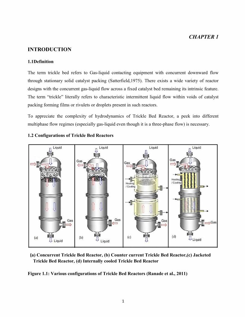
1.2 Configurations of Trickle Bed Reactors

Figure 1.1: Various configurations of Trickle Bed Reactors (Ranade et al., 2011)

(a) Concurrent Trickle Bed Reactor, (b) Counter current Trickle Bed Reactor,(c) Jacketed

Trickle Bed Reactor, (d) Internally cooled Trickle Bed Reactor

2

Trickle bed reactors are generally used in four different configuration setups based upon packing

structure (Ranade et al., 2011):

a. Concurrent Trickle Bed Reactor

b. Counter current Trickle Bed Reactor

c. Jacketed Trickle Bed Reactor

d. Internally cooled Trickle Bed Reactor

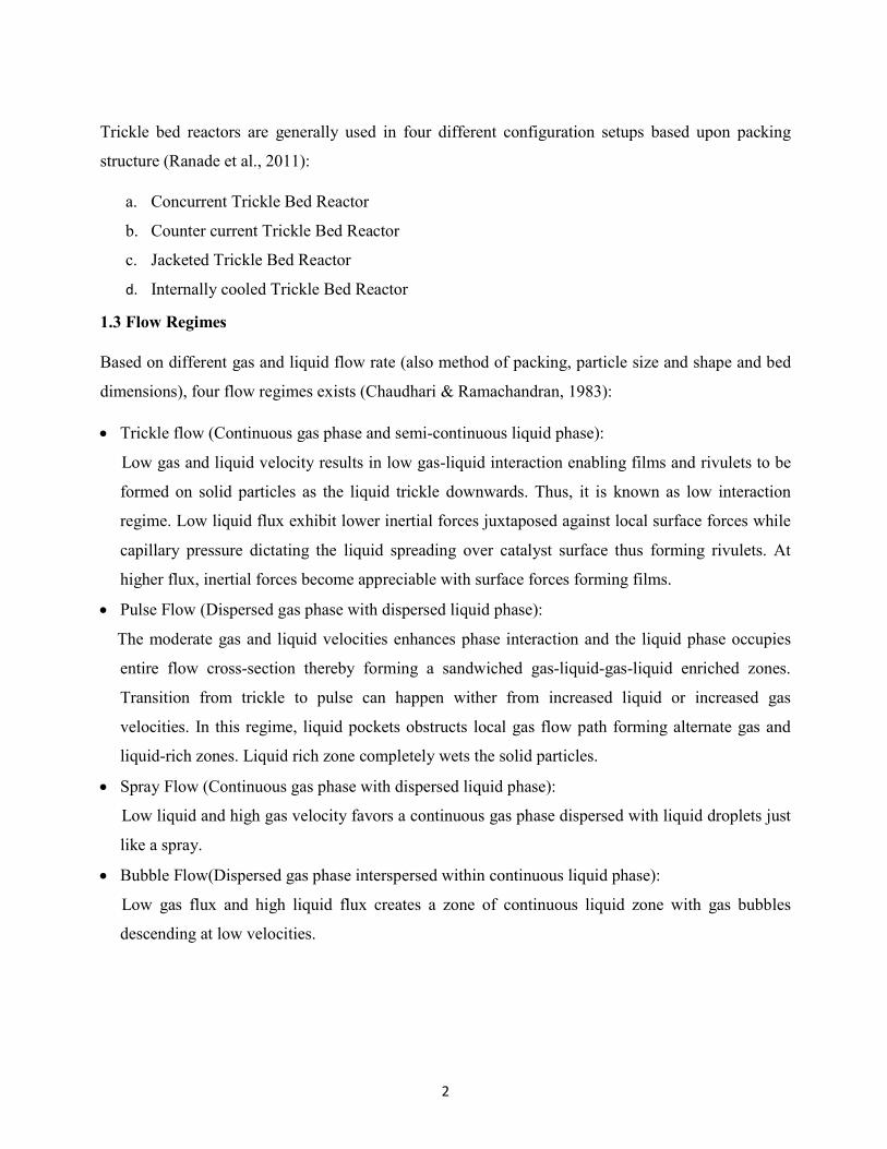
1.3 Flow Regimes

Based on different gas and liquid flow rate (also method of packing, particle size and shape and bed

dimensions), four flow regimes exists (Chaudhari & Ramachandran, 1983):

Trickle flow (Continuous gas phase and semi-continuous liquid phase):

Low gas and liquid velocity results in low gas-liquid interaction enabling films and rivulets to be

formed on solid particles as the liquid trickle downwards. Thus, it is known as low interaction

regime. Low liquid flux exhibit lower inertial forces juxtaposed against local surface forces while

capillary pressure dictating the liquid spreading over catalyst surface thus forming rivulets. At

higher flux, inertial forces become appreciable with surface forces forming films.

Pulse Flow (Dispersed gas phase with dispersed liquid phase):

The moderate gas and liquid velocities enhances phase interaction and the liquid phase occupies

entire flow cross-section thereby forming a sandwiched gas-liquid-gas-liquid enriched zones.

Transition from trickle to pulse can happen wither from increased liquid or increased gas

velocities. In this regime, liquid pockets obstructs local gas flow path forming alternate gas and

liquid-rich zones. Liquid rich zone completely wets the solid particles.

Spray Flow (Continuous gas phase with dispersed liquid phase):

Low liquid and high gas velocity favors a continuous gas phase dispersed with liquid droplets just

like a spray.

Bubble Flow(Dispersed gas phase interspersed within continuous liquid phase):

Low gas flux and high liquid flux creates a zone of continuous liquid zone with gas bubbles

descending at low velocities.

3

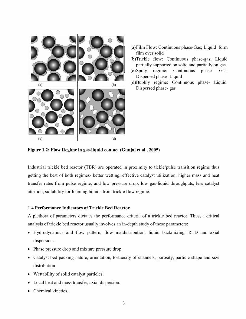
Figure 1.2: Flow Regime in gas-liquid contact (Gunjal et al., 2005)

Industrial trickle bed reactor (TBR) are operated in proximity to tickle/pulse transition regime thus

getting the best of both regimes- better wetting, effective catalyst utilization, higher mass and heat

transfer rates from pulse regime; and low pressure drop, low gas-liquid throughputs, less catalyst

attrition, suitability for foaming liquids from trickle flow regime.

1.4 Performance Indicators of Trickle Bed Reactor

A plethora of parameters dictates the performance criteria of a trickle bed reactor. Thus, a critical

analysis of trickle bed reactor usually involves an in-depth study of these parameters:

Hydrodynamics and flow pattern, flow maldistribution, liquid backmixing, RTD and axial

dispersion.

Phase pressure drop and mixture pressure drop.

Catalyst bed packing nature, orientation, tortuosity of channels, porosity, particle shape and size

distribution

Wettability of solid catalyst particles.

Local heat and mass transfer, axial dispersion.

Chemical kinetics.

(a) Film Flow: Continuous phase-Gas; Liquid form film over solid

(b) Trickle flow: Continuous phase-gas; Liquid partially supported on solid and partially on gas

(c) Spray regime: Continuous phase- Gas, Dispersed phase- Liquid

(d) Bubbly regime: Continuous phase- Liquid, Dispersed phase- gas

4

1.5 Advantages and Disadvantages of Trickle Bed Reactor

Many chemical industries rely on trickle bed reactor (TBR) because:

It’s simple design and operation procedure under severe environment is its forte making it suitable

for industrial-scale production (Ranade et al.,2011).

No need for additional catalyst separation unit also minimizes catalyst attrition.

It can accept solid catalyst with a wider range of size and shape which makes it versatile.

The design of trickle-bed helps in exploiting the benefits of plug flow scenario better than slurry

bubble or packed or stirred reactor leading to higher conversion and selectivity.

Large-scale operation is more economical in trickle bed reactor than any other type of reactors.

No concern for flooding has to be considered because of concurrent gas and liquid flow.

Lower liquid holdup (or higher catalyst holdup) favors minimizing homogeneous liquid phase

reaction which is attained in trickle bed reactor as compared to ebulliating bed or slurry bed reactor.

This also leads to higher throughput per unit volume of reactor for large catalyst holdup.

Unlike fluidized bed, slurry bed or stirred reactor, power consumption is quite lower as there is no

need for solid to be suspended.

It has lesser pressure drop and lesser back-mixing than packed beds.

Still there are some shortcomings restricting the extensive use of trickle bed reactor which are:

Lower intraparticle and interphase mass and heat transfer limits reaction rate.

Incomplete wetting and liquid maldistribution as a result from low liquid velocity decreases overall

performance of reactor. Liquid maldistribution may results from- improper initial feed distribution,

randomness in local properties of packing, wall effects, wetting properties of catalyst, intrinsic

properties of liquid and severity of operating conditions (Schwidder & Schnitzlein, 2012).

Partial wetting of catalyst can wreak havoc in trickle bed reactor operations by causing undesirable

gas phase side reactions, hot-spot formation or temperature runaways. This issue can be mitigated by

using intermediate cooling, excess solvent and liquid distributors. This limits the use of trickle bed

reactor in slower reactions requiring high catalyst loading.

Radial heat and mass flux may seem to be a problem.

However, there is further scope of optimization of trickle bed reactor performance which can be

realized with more comprehensive research works.

5

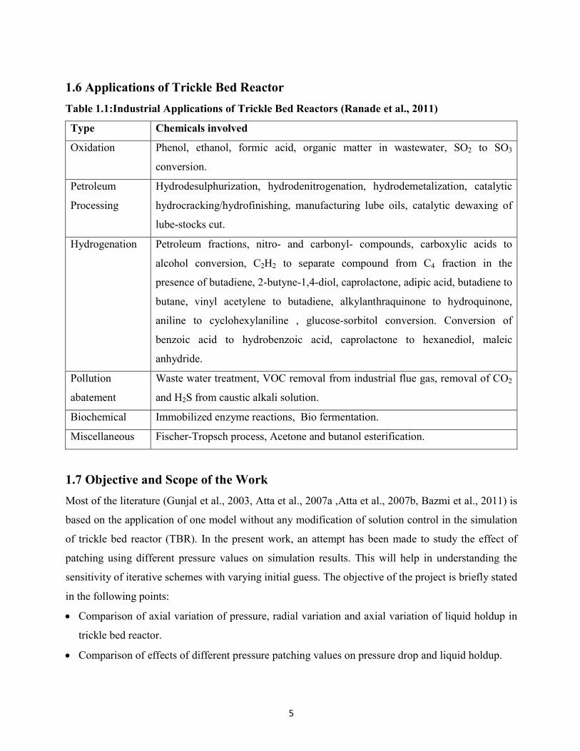
1.6 Applications of Trickle Bed Reactor

Table 1.1:Industrial Applications of Trickle Bed Reactors (Ranade et al., 2011)

Type Chemicals involved

Oxidation Phenol, ethanol, formic acid, organic matter in wastewater, SO2 to SO3

conversion.

Petroleum

Processing

Hydrodesulphurization, hydrodenitrogenation, hydrodemetalization, catalytic

hydrocracking/hydrofinishing, manufacturing lube oils, catalytic dewaxing of

lube-stocks cut.

Hydrogenation Petroleum fractions, nitro- and carbonyl- compounds, carboxylic acids to

alcohol conversion, C2H2 to separate compound from C4 fraction in the

presence of butadiene, 2-butyne-1,4-diol, caprolactone, adipic acid, butadiene to

butane, vinyl acetylene to butadiene, alkylanthraquinone to hydroquinone,

aniline to cyclohexylaniline , glucose-sorbitol conversion. Conversion of

benzoic acid to hydrobenzoic acid, caprolactone to hexanediol, maleic

anhydride.

Pollution

abatement

Waste water treatment, VOC removal from industrial flue gas, removal of CO2

and H2S from caustic alkali solution.

Biochemical Immobilized enzyme reactions, Bio fermentation.

Miscellaneous Fischer-Tropsch process, Acetone and butanol esterification.

1.7 Objective and Scope of the Work

Most of the literature (Gunjal et al., 2003, Atta et al., 2007a ,Atta et al., 2007b, Bazmi et al., 2011) is

based on the application of one model without any modification of solution control in the simulation

of trickle bed reactor (TBR). In the present work, an attempt has been made to study the effect of

patching using different pressure values on simulation results. This will help in understanding the

sensitivity of iterative schemes with varying initial guess. The objective of the project is briefly stated

in the following points:

Comparison of axial variation of pressure, radial variation and axial variation of liquid holdup in

trickle bed reactor.

Comparison of effects of different pressure patching values on pressure drop and liquid holdup.

6

CHAPTER 2

LITERATURE REVIEW

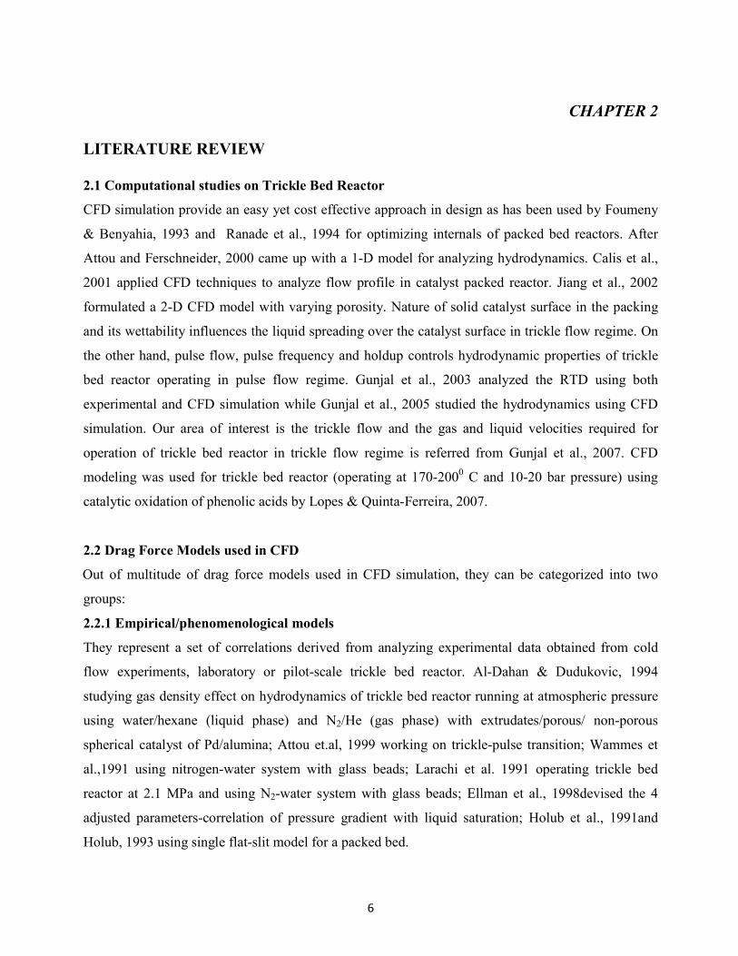
2.1 Computational studies on Trickle Bed Reactor

CFD simulation provide an easy yet cost effective approach in design as has been used by Foumeny

& Benyahia, 1993 and Ranade et al., 1994 for optimizing internals of packed bed reactors. After

Attou and Ferschneider, 2000 came up with a 1-D model for analyzing hydrodynamics. Calis et al.,

2001 applied CFD techniques to analyze flow profile in catalyst packed reactor. Jiang et al., 2002

formulated a 2-D CFD model with varying porosity. Nature of solid catalyst surface in the packing

and its wettability influences the liquid spreading over the catalyst surface in trickle flow regime. On

the other hand, pulse flow, pulse frequency and holdup controls hydrodynamic properties of trickle

bed reactor operating in pulse flow regime. Gunjal et al., 2003 analyzed the RTD using both

experimental and CFD simulation while Gunjal et al., 2005 studied the hydrodynamics using CFD

simulation. Our area of interest is the trickle flow and the gas and liquid velocities required for

operation of trickle bed reactor in trickle flow regime is referred from Gunjal et al., 2007. CFD

modeling was used for trickle bed reactor (operating at 170-2000 C and 10-20 bar pressure) using

catalytic oxidation of phenolic acids by Lopes & Quinta-Ferreira, 2007.

2.2 Drag Force Models used in CFD

Out of multitude of drag force models used in CFD simulation, they can be categorized into two

groups:

2.2.1 Empirical/phenomenological models

They represent a set of correlations derived from analyzing experimental data obtained from cold

flow experiments, laboratory or pilot-scale trickle bed reactor. Al-Dahan & Dudukovic, 1994

studying gas density effect on hydrodynamics of trickle bed reactor running at atmospheric pressure

using water/hexane (liquid phase) and N2/He (gas phase) with extrudates/porous/ non-porous

spherical catalyst of Pd/alumina; Attou et.al, 1999 working on trickle-pulse transition; Wammes et

al.,1991 using nitrogen-water system with glass beads; Larachi et al. 1991 operating trickle bed

reactor at 2.1 MPa and using N2-water system with glass beads; Ellman et al., 1998devised the 4

adjusted parameters-correlation of pressure gradient with liquid saturation; Holub et al., 1991and

Holub, 1993 using single flat-slit model for a packed bed.

7

2.2.2 Semi-empirical models

Attou et al., 1999 proposed this model to describe the hydrodynamics involved in trickle bed reactor

and is based on macroscopic ensemble-average mass and momentum conservation laws. Interphase

drag is calculated from theoretical standpoint. However, the weak point of the model is that it

underestimates the pressure gradient at higher superficial gas velocities.

Succinctly, there are three widely adopted models used for calculating drag force expression. As

stated by Carbonell, 2000, they are as follows:

Relative permeability model by Saez and Carbonell, 1985

The slit model by Holub et al., 1992 and 1993

Fluid-fluid interaction model by Attou and Boyer, 1999

2.2.2.1 Relative Permeability model

Derived by Saez and Carbonell,1985 this model has gain a wide acceptance in many engineering

fields like soil science, textile engineering, pollution abatement and environmental science, chemical

science, reservoir engineering, fuel cells, subsurface environmental engineering and has an ever-

increasing popularity in research community (Xiao et al., 2012). Relative permeability of phase is

considered as the tendency of one fluid to flow with respect to motion of another fluid and thus

modifies drag force expression for on phase flow. Relative permeability is dependent on phase

holdup and saturation of corresponding phase.

2.2.2.2 Slit Model

Representing the fluid flow around solid packing of trickle-bed as flow through a rectangular slit, this

model also include slip effect to calculate velocity and stress fields. As Holub et al., 1992, 1993 states

that the slit gap depends on voidage of porous medium, and the orientation of slit is related to

tortuosity factor for the packed bed.

2.2.2.3 Fluid-Fluid Interaction Model

Macroscopic mass and momentum balance is applicable over control volume in interstitial space

between solid particles. This model is consistent for incompressible two-phase, two species

concurrent gas-liquid trickle flow; 1-D, steady state, 2-phase flow with Newtonian fluids. Momentum

exchange terms are calculated from Ergun’s equation (modified form for multiphase flow).

8

CHAPTER 3

CFD Modeling

3.1 Definition of CFD

CFD is a novel technique to simulate fluid engineering system and involves predicting fluid flow,

heat transfer, mass transfer, chemical reactions and related phenomena by solving governing

mathematical equations by numerical methods.

Results from CFD helps in achieving some of the required objectives like:

Conceptual study of new design

Detailed product development

Troubleshooting

Redesign

3.2 Basic Governing Equations

Mathematical modeling of any physical system involves a set of characteristic equations like:

Conservative form of equations

Equations based on basic thermodynamic laws

Equation of state

Equations relating intrinsic properties of the system (like Newton’s law of motion, Newton’s

viscosity relation, Fourier law of heat conduction, Law of gravitation)

Out of which the conservative equations play a central role and are indispensible to any physical

system. And for fluid flow system, they are:

Equation of continuity:

+ ∇. () = 0 (3.1)

Equation of motion:

() + ∇. () = −∇ + ∇. [μ(∇ + ∇

)] + + + ∇. (,

. ,)

(3.2)

9

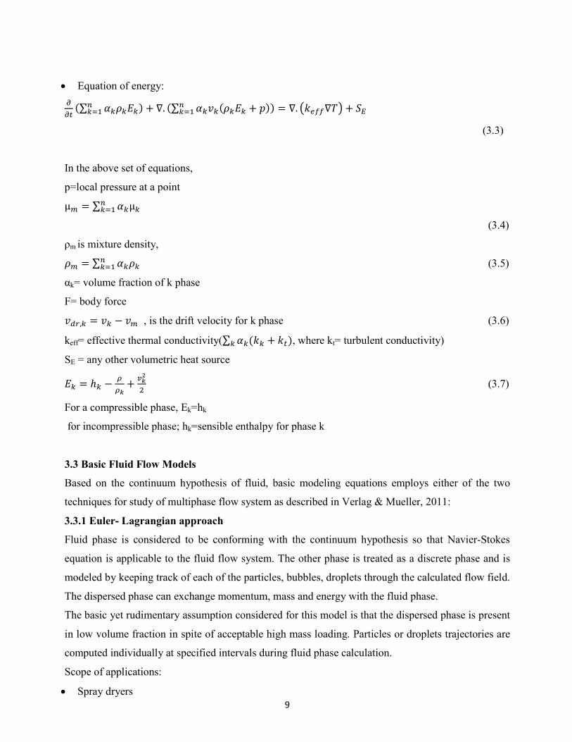
Equation of energy:

(∑

) + ∇. (∑ ( + )

) = ∇. ∇+

(3.3)

In the above set of equations,

p=local pressure at a point

μ = ∑ μ

(3.4)

ρm is mixture density,

= ∑ (3.5)

αk= volume fraction of k phase

F= body force

, = − , is the drift velocity for k phase (3.6)

keff= effective thermal conductivity(∑ ( + ) , where kt= turbulent conductivity)

SE = any other volumetric heat source

= ℎ −

+

(3.7)

For a compressible phase, Ek=hk

for incompressible phase; hk=sensible enthalpy for phase k

3.3 Basic Fluid Flow Models

Based on the continuum hypothesis of fluid, basic modeling equations employs either of the two

techniques for study of multiphase flow system as described in Verlag & Mueller, 2011:

3.3.1 Euler- Lagrangian approach

Fluid phase is considered to be conforming with the continuum hypothesis so that Navier-Stokes

equation is applicable to the fluid flow system. The other phase is treated as a discrete phase and is

modeled by keeping track of each of the particles, bubbles, droplets through the calculated flow field.

The dispersed phase can exchange momentum, mass and energy with the fluid phase.

The basic yet rudimentary assumption considered for this model is that the dispersed phase is present

in low volume fraction in spite of acceptable high mass loading. Particles or droplets trajectories are

computed individually at specified intervals during fluid phase calculation.

Scope of applications:

Spray dryers

10

Coal and liquid fuel combustion

Particle-laden flow but not for liquid-liquid mixtures, fluidized beds or any application where

volume fraction of second phase

3.3.2 Euler- Euler approach:

Different phases are represented in mathematical modeling as interpenetrating continua where any

space in computational domain is exclusively occupied by either one of the many phases. This gives

rise to the concept of phasic volume fraction, which itself are a continuous spatial-temporal functions

and sums up to unity. Conservation equations are formulated for each phases which in turns yields a

set of equations. The closure of the equations is provided from using empirical information, or in

case of granular flows, by implementing kinetic theory.

Out of the above two approaches, we adopt the second one for the reason of

Three forms of Euler-Euler approach of modeling:

Volume of Fluid (VOF) model

Mixture model

Eulerian model

3.3.2.1 Volume of Fluid Model

For a system of immiscible fluids, VOF model is used which solves a set of momentum equation and

analyzing the surface volume fraction of the fluids used in computational domain. While VOF model

finds wide application in case of time-dependent solution, the steady stated from is also used. This

model assumes the non-penetrating nature of the fluids. Area of application if the model includes

liquid jet breakup prediction, motion of large bubbles inside liquid, stratified flows, liquid flow after

dam break, steady or transient tracking of nay gas-liquid interface. Some of its limitation includes:

Available only for pressure-based solver.

Inability to model streamwise periodic flow.

Second-order implicit time-splitting step cannot run in this model.

3.3.2.2 Mixture Model

On the assumption of two fluids behaving as interpenetrating continua moving at different velocities,

mixture model calculates relative velocities for dispersed phases to model homogeneous flow.

However, it also assumes local equilibrium over short length scales. Applications include particle-

laden flow with low loading, sedimentation, cyclone separator.

11

3.3.2.3 Eulerian Model

The Eulerian model solves n sets of equations for each phase. The pressure and interphase exchange

coefficients incorporates the coupling effects. The nature of phases involved dictates the mode of

handling coupling by this model. There is a separate technique for handling granular and non-

granular flows. The properties of phases described as “granular” flow are derived from kinetic

theory. Momentum exchange between the phases is influenced by the nature of the phases. UDF

(User-defined functions) also comes handy when momentum exchange is to be calculated. Eulerian

models mostly find use in areas such as bubble columns, risers, particle suspension and fluidized

beds, packed beds and trickle bed reactors. A detailed guideline and criterions are listed in the

ANSYS theory guide to help choose which model can be used in a particular scenario.

3.4 Drag Force Calculation:

This project deals with gas-liquid system and as common perception, gas phase should travel faster

than the liquid phase. This results in phase slippage and culminates into interphase drag force, a

parameter that plays a pivotal role in turbulence modeling. To understand this concept, the term

relative velocity has been introduced; which is defined as difference between primary phase and

secondary phase velocity (that is p and q); also

= − (3.8)

For the multiphase system, we have the following options for drag force calculation:

Schiller-Nauman model which calculates the drag coefficients based on the range of Reynolds

number and then calculate the friction factor from Drag coefficient. This is generally used in case

of fluid-fluid drag function.

Gidaspow et al. calculates the momentum exchange coefficients for each pair of phases using the

drag coeeficients. It uses Ergun type equations for packing with bed voidage less than 0.8 while

Wen yu equation is used for higher bed voidage.

3.5 Turbulence Model (the k- ε model )

Due to chaotic nature of turbulence, there has to be a multitude of models to represent the exact

nature of turbulent flow for each specific scenario. Dealing with RANS-based turbulence model is

comparatively easy for CFD simulation and is widely applicable in many scenarios. Sophisticated

models like LES, DES and DNS models are applicable for highly sophisticated problems dealing

with big data. The linear, non-linear eddy viscosity models and Reynolds Stress Model forms the

RANS-based model. While the non-linear eddy viscosity models (EVM) can truly represent

12

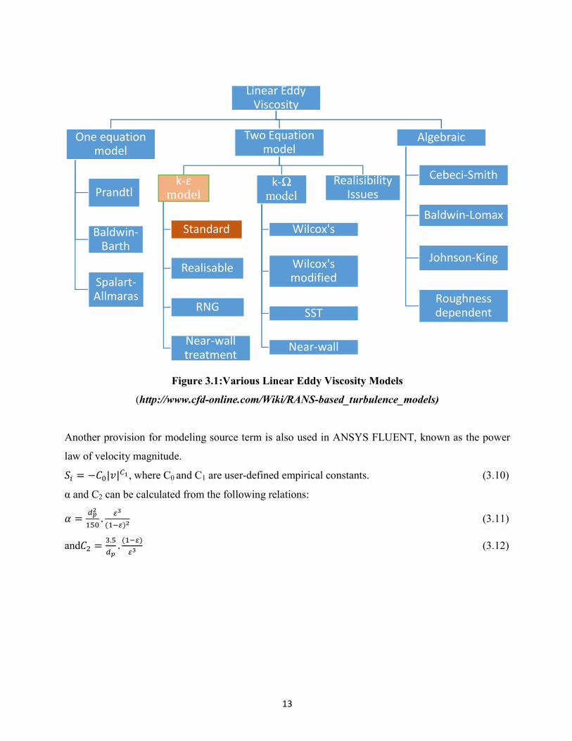
turbulence in the system, they are most complex and hence less popular in CFD. Our main focus in

CFD is the linear eddy viscosity models which are available in different forms as shown in Figure

3.1.

The two-equation model computes two parameters- turbulent length and time-scale from two

different transport equations. The standard k-ε model belongs to the two-equation model category.

Proposed by Launder and Spalding, it is based on kinetic energy (k) and its dissipation (ε). Basic

assumptions considered are: a fully turbulent flow and miniscule effect of molecular viscosity.

It suffers from the disadvantage of high insensitivity to abnormal pressure gradient and boundary

layer separation. They prognosticate a deferred and condensed separation with respect to observer

leading to overly optimistic modeling. The turbulence kinetic energy arises from two effects: from

the mean velocity gradient and the buoyancy effects. While the RNG form of k- ε model uses the

statistical approach called the renormalized group, the Realizable form solves equations within

constraints put on Reynolds stresses.

3.6 Porous Media Model:

It finds application in packed beds, tube banks, perforated plates, catalytic convertors, mixing tank

problems and many more scenarios. Initially, the phase (cell zone) on which porous media model is

to be applied is specified. Pressure loss is calculated too based on the inputs like the Superficial

Velocity Porous Formulation (indication of bulk pressure loss). Superficial velocity is same whether

the region is inside the porous zone or outside of it. This curtails its velocity increase computation

capability to some extent and hence limits its accuracy. This model incorporates an additional term- a

momentum source term to transport equations. This source term comprises of two parts: a viscous

resistance term (Darcy’s term) and an inertial resistance term (Forschneider term).The present

problem in focus is a case of homogeneous porous media where porous media model is of the form:

= −(

+

||) , where α= permeability and C2= internal resistance factor. (3.9)

13

Figure 3.1:Various Linear Eddy Viscosity Models

(http://www.cfd-online.com/Wiki/RANS-based_turbulence_models)

Another provision for modeling source term is also used in ANSYS FLUENT, known as the power

law of velocity magnitude.

= −||, where C0 and C1 are user-defined empirical constants. (3.10)

α and C2 can be calculated from the following relations:

=

.

() (3.11)

and =.

.()

(3.12)

Linear Eddy Viscosity

One equation model

Prandtl

Baldwin-Barth

Spalart-Allmaras

Two Equation model

k-εmodel

Standard

Realisable

RNG

Near-wall treatment

k-Ωmodel

Wilcox's

Wilcox's modified

SST

Near-wall

Realisibility Issues

Algebraic

Cebeci-Smith

Baldwin-Lomax

Johnson-King

Roughness dependent

14

CHAPTER 4

CFD SIMULATION

The geometry is prepared using ANSYS Design Modeler. Subsequently, mesh is prepared with the

help of ANSYS Meshing application and then run in ANSYS® FLUENT 15.0. A comparison is

drawn on the results (obtained from ANSYS CFD-Post) of various models and varying phasic

velocities. Results are analyzed and plotted using Origin Pro 2015. The whole project focuses on

trickle flow regime only.

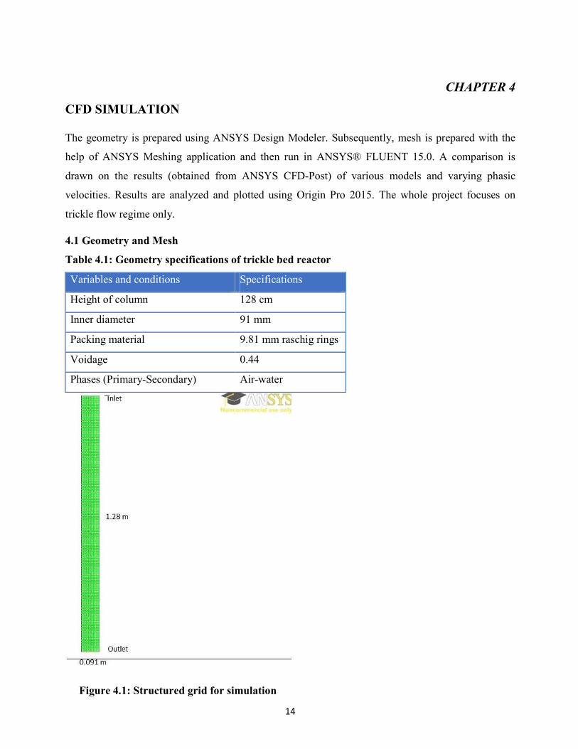
4.1 Geometry and Mesh

Table 4.1: Geometry specifications of trickle bed reactor

Variables and conditions Specifications

Height of column 128 cm

Inner diameter 91 mm

Packing material 9.81 mm raschig rings

Voidage 0.44

Phases (Primary-Secondary) Air-water

Figure 4.1: Structured grid for simulation

15

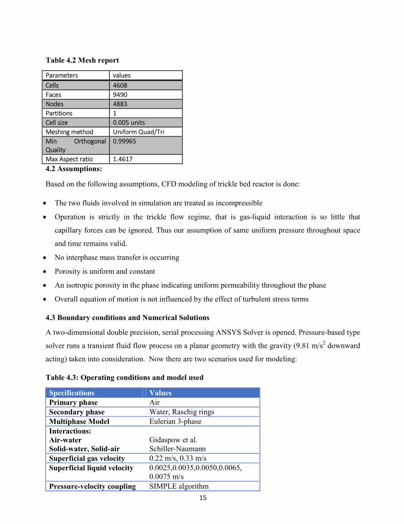
Table 4.2 Mesh report

Parameters values

Cells 4608

Faces 9490

Nodes 4883

Partitions 1

Cell size 0.005 units

Meshing method Uniform Quad/Tri

Min Orthogonal Quality

0.99965

Max Aspect ratio 1.4617

4.2 Assumptions:

Based on the following assumptions, CFD modeling of trickle bed reactor is done:

The two fluids involved in simulation are treated as incompressible

Operation is strictly in the trickle flow regime, that is gas-liquid interaction is so little that

capillary forces can be ignored. Thus our assumption of same uniform pressure throughout space

and time remains valid.

No interphase mass transfer is occurring

Porosity is uniform and constant

An isotropic porosity in the phase indicating uniform permeability throughout the phase

Overall equation of motion is not influenced by the effect of turbulent stress terms

4.3 Boundary conditions and Numerical Solutions

A two-dimensional double precision, serial processing ANSYS Solver is opened. Pressure-based type

solver runs a transient fluid flow process on a planar geometry with the gravity (9.81 m/s2 downward

acting) taken into consideration. Now there are two scenarios used for modeling:

Table 4.3: Operating conditions and model used

Specifications Values Primary phase Air Secondary phase Water, Raschig rings

Multiphase Model Eulerian 3-phase

Interactions: Air-water Solid-water, Solid-air

Gidaspow et al. Schiller-Naumann

Superficial gas velocity 0.22 m/s, 0.33 m/s

Superficial liquid velocity 0.0025,0.0035,0.0050,0.0065, 0.0075 m/s

Pressure-velocity coupling SIMPLE algorithm

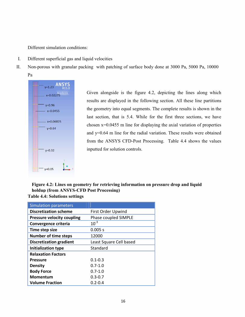
Different simulation conditions:

I. Different superficial gas and liquid velocities

II. Non-porous with granular packing with patching of surface body done at

Pa

Table 4.4: Solutions settings

Simulation parameters

Discretization scheme

Pressure velocity coupling

Convergence criteria

Time step size

Number of time steps

Discretization gradient

Initialization type

Relaxation Factors Pressure Density Body Force Momentum Volume Fraction

Given alongside is the figure

results are displayed in the following section. All these line partitions

the geometry

last section, that is 5.4. While for the first three sections,

chosen

and y=0.64 m line for the

from the ANSYS

inputted for solution controls.

Figure 4.2: Lines on geometry for retrieving information on pressure drop and liquid holdup (from ANSYS-CFD Post Processing)

16

Different superficial gas and liquid velocities

porous with granular packing with patching of surface body done at 3000 Pa, 5

First Order Upwind

Phase coupled SIMPLE

10-3

0.005 s

12000

Least Square Cell based

Standard

0.1-0.3 0.7-1.0 0.7-1.0 0.3-0.7 0.2-0.4

Given alongside is the figure 4.2, depicting the lines along which

results are displayed in the following section. All these line partitions

the geometry into equal segments. The complete results is shown in the

last section, that is 5.4. While for the first three sections,

chosen x=0.0455 m line for displaying the axial

and y=0.64 m line for the radial variation. These resul

from the ANSYS CFD-Post Processing. Table 4.4 shows the values

inputted for solution controls.

metry for retrieving information on pressure drop and liquid CFD Post Processing)

3000 Pa, 5000 Pa, 10000

depicting the lines along which

results are displayed in the following section. All these line partitions

into equal segments. The complete results is shown in the

last section, that is 5.4. While for the first three sections, we have

variation of properties

variation. These results were obtained

Table 4.4 shows the values

metry for retrieving information on pressure drop and liquid

17

CHAPTER 5

RESULTS AND DISCUSSION

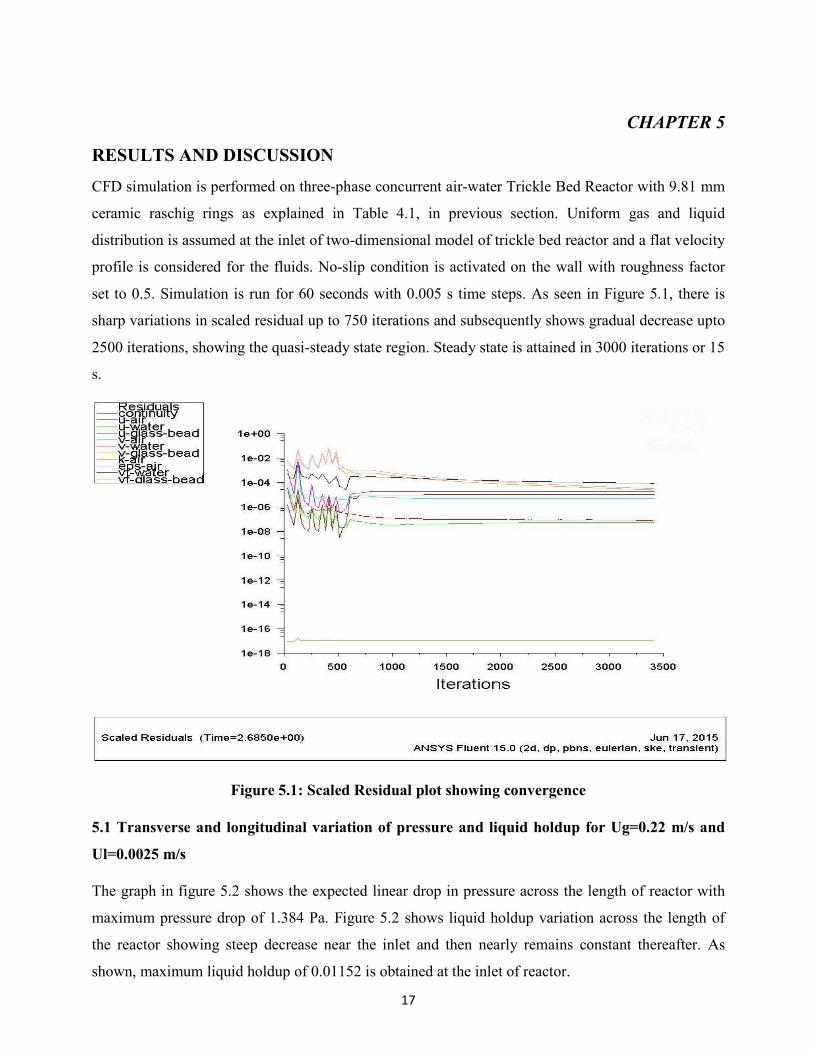
CFD simulation is performed on three-phase concurrent air-water Trickle Bed Reactor with 9.81 mm

ceramic raschig rings as explained in Table 4.1, in previous section. Uniform gas and liquid

distribution is assumed at the inlet of two-dimensional model of trickle bed reactor and a flat velocity

profile is considered for the fluids. No-slip condition is activated on the wall with roughness factor

set to 0.5. Simulation is run for 60 seconds with 0.005 s time steps. As seen in Figure 5.1, there is

sharp variations in scaled residual up to 750 iterations and subsequently shows gradual decrease upto

2500 iterations, showing the quasi-steady state region. Steady state is attained in 3000 iterations or 15

s.

Figure 5.1: Scaled Residual plot showing convergence

5.1 Transverse and longitudinal variation of pressure and liquid holdup for Ug=0.22 m/s and

Ul=0.0025 m/s

The graph in figure 5.2 shows the expected linear drop in pressure across the length of reactor with

maximum pressure drop of 1.384 Pa. Figure 5.2 shows liquid holdup variation across the length of

the reactor showing steep decrease near the inlet and then nearly remains constant thereafter. As

shown, maximum liquid holdup of 0.01152 is obtained at the inlet of reactor.

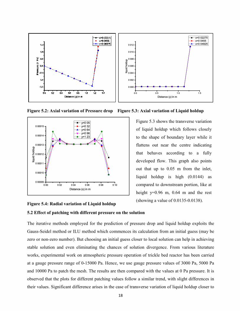
Figure 5.2: Axial variation of Pressure drop

Figure 5.4: Radial variation of

5.2 Effect of patching with different pressure on the solution

The iterative methods employed for the prediction of pressure drop and liquid holdup exploits the

Gauss-Seidel method or ILU method which commences its calculation from an initial guess (may be

zero or non-zero number). But choosing

stable solution and even eliminating the chances of solution divergence.

works, experimental work on atmospheric pressure operation of

at a gauge pressure range of 0-15000 Pa.

and 10000 Pa to patch the mesh. The resul

observed that the plots for different patching values follow a similar trend, with slight differences in

their values. Significant difference arises in the case of

18

: Axial variation of Pressure drop Figure 5.3: Axial variation of

: Radial variation of Liquid holdup

Effect of patching with different pressure on the solution

The iterative methods employed for the prediction of pressure drop and liquid holdup exploits the

method which commences its calculation from an initial guess (may be

choosing an initial guess closer to local solution can help in achieving

stable solution and even eliminating the chances of solution divergence. From

works, experimental work on atmospheric pressure operation of trickle bed reactor

15000 Pa. Hence, we use gauge pressure values of 3000 Pa, 5000 Pa

to patch the mesh. The results are then compared with the values at 0 Pa pressure.

observed that the plots for different patching values follow a similar trend, with slight differences in

ifference arises in the case of transverse variation of liquid

Figure 5.3 shows the transverse variation

of liquid holdup which follows closely

to the shape of boundary layer while it

flattens out near the

that behaves according to a fully

developed flow. This graph also points

out that up to 0.05 m from the inlet,

liquid holdup is high (0.0144) as

compared to downstream portion, like at

height y=0.96 m, 0.64 m and the rest

(showing a value of 0.0135

riation of Liquid holdup

The iterative methods employed for the prediction of pressure drop and liquid holdup exploits the

method which commences its calculation from an initial guess (may be

an initial guess closer to local solution can help in achieving

From various literature

trickle bed reactor has been carried

we use gauge pressure values of 3000 Pa, 5000 Pa

ts are then compared with the values at 0 Pa pressure. It is

observed that the plots for different patching values follow a similar trend, with slight differences in

liquid holdup closer to

the transverse variation

which follows closely

to the shape of boundary layer while it

flattens out near the centre indicating

that behaves according to a fully

This graph also points

out that up to 0.05 m from the inlet,

liquid holdup is high (0.0144) as

compared to downstream portion, like at

height y=0.96 m, 0.64 m and the rest

e of 0.0135-0.0138).

19

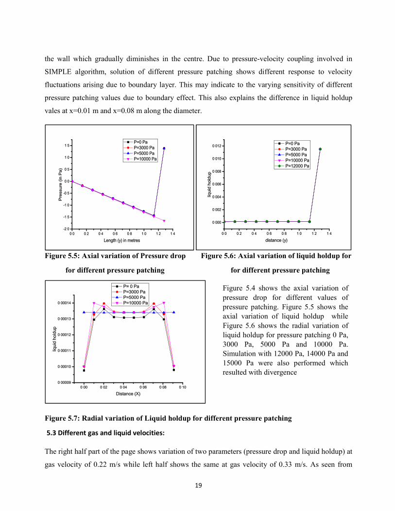
the wall which gradually diminishes in the centre. Due to pressure-velocity coupling involved in

SIMPLE algorithm, solution of different pressure patching shows different response to velocity

fluctuations arising due to boundary layer. This may indicate to the varying sensitivity of different

pressure patching values due to boundary effect. This also explains the difference in liquid holdup

vales at x=0.01 m and x=0.08 m along the diameter.

Figure 5.5: Axial variation of Pressure drop Figure 5.6: Axial variation of liquid holdup for

for different pressure patching for different pressure patching

Figure 5.7: Radial variation of Liquid holdup for different pressure patching

5.3 Different gas and liquid velocities:

The right half part of the page shows variation of two parameters (pressure drop and liquid holdup) at

gas velocity of 0.22 m/s while left half shows the same at gas velocity of 0.33 m/s. As seen from

Figure 5.4 shows the axial variation of

pressure drop for different values of pressure patching. Figure 5.5 shows the axial variation of liquid holdup while Figure 5.6 shows the radial variation of liquid holdup for pressure patching 0 Pa, 3000 Pa, 5000 Pa and 10000 Pa. Simulation with 12000 Pa, 14000 Pa and 15000 Pa were also performed which resulted with divergence

20

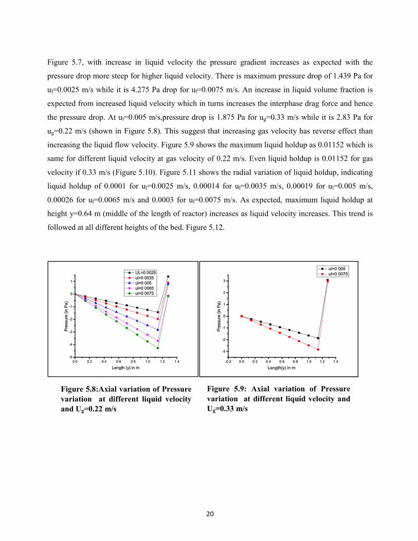
Figure 5.7, with increase in liquid velocity the pressure gradient increases as expected with the

pressure drop more steep for higher liquid velocity. There is maximum pressure drop of 1.439 Pa for

ul=0.0025 m/s while it is 4.275 Pa drop for ul=0.0075 m/s. An increase in liquid volume fraction is

expected from increased liquid velocity which in turns increases the interphase drag force and hence

the pressure drop. At ul=0.005 m/s,pressure drop is 1.875 Pa for ug=0.33 m/s while it is 2.83 Pa for

ug=0.22 m/s (shown in Figure 5.8). This suggest that increasing gas velocity has reverse effect than

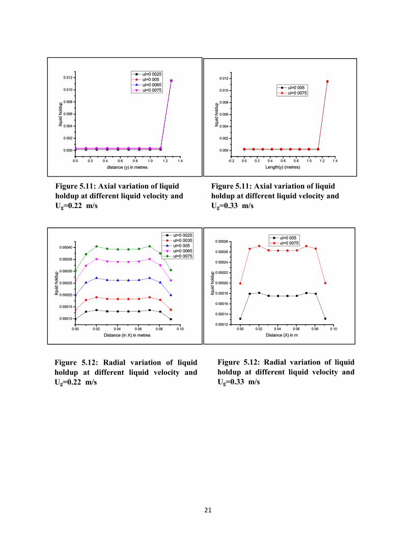
increasing the liquid flow velocity. Figure 5.9 shows the maximum liquid holdup as 0.01152 which is

same for different liquid velocity at gas velocity of 0.22 m/s. Even liquid holdup is 0.01152 for gas

velocity if 0.33 m/s (Figure 5.10). Figure 5.11 shows the radial variation of liquid holdup, indicating

liquid holdup of 0.0001 for ul=0.0025 m/s, 0.00014 for ul=0.0035 m/s, 0.00019 for ul=0.005 m/s,

0.00026 for ul=0.0065 m/s and 0.0003 for ul=0.0075 m/s. As expected, maximum liquid holdup at

height y=0.64 m (middle of the length of reactor) increases as liquid velocity increases. This trend is

followed at all different heights of the bed. Figure 5.12.

Figure 5.8:Axial variation of Pressure variation at different liquid velocity and Ug=0.22 m/s

Figure 5.9: Axial variation of Pressure

variation at different liquid velocity and Ug=0.33 m/s

21

igure 5.1 Pressure drop along y

Figure 5.11: Axial variation of liquid holdup at different liquid velocity and Ug=0.22 m/s

Figure 5.11: Axial variation of liquid holdup at different liquid velocity and Ug=0.33 m/s

Figure 5.12: Radial variation of liquid holdup at different liquid velocity and Ug=0.22 m/s

Figure 5.12: Radial variation of liquid holdup at different liquid velocity and Ug=0.33 m/s

22

CHAPTER 6

CONCLUSION

A two-dimensional model for trickle bed reactor is solved using ANSYS employing the Eulerian-

Eulerian model with specifications of the trickle bed reactor as mentioned in Table 4.1 in previous

section. For gas velocity of 0.22 m/s, we run simulation for different liquid velocities of 0.0025 m/s,

0.0035 m/s, 0.005 m/s, 0.0065 m/s and 0.0075 m/s. On the other hand, for gas velocity of 0.33 m/s,

we have results for 0.005 m/s and 0.0075 m/s liquid velocities. From the different case scenario of

the ANSYS simulation of trickle bed reactor, we can infer that:

Pressure decreases linearly along length of the reactor and more is the liquid velocity, steeper is

the pressure drop. Pressure drop increases with decreasing gas velocity and increasing liquid

velocity. Patching values have no effect up to a certain range, which is 10000 Pa. Beyond the

10000 Pa value, the solution becomes instable as is expected from the limitations of iterative

schemes. Divergence is detected which cannot be eliminated. The sharp increase in pressure drop

close to the inlet is maybe due to excessive pressure loss in the entrance length.

Liquid holdup has strong variation in transverse section, following the usual fully developed

turbulent flow regime. This is shown by the two portion of the radial liquid holdup variation plot,

one in which consists of flatter region (within 0.03-0.06 m) resembling the turbulent core section

of fully developed flow; the second one is the sharply varying hump like section within 0.03 m

from the wall resembling the boundary layer. Axial variation shows that liquid holdup decreases

steeply (from 0.01152 to 0.00026) close to the inlet than in any other portion of the reactor. For

different patching pressure values, the radial variation of liquid holdup follows the same line,

while the radial variation of liquid holdup shows slight deviation at x=0.03 and x=0.06 m.

Future scope of the work

For an extensive study of hydrodynamics of trickle bed reactors, a comparison of all the three models

(relative permeability, slit model, fluid-fluid interaction model) on a Trickle-Bed reactor operating at

high pressure high temperature can be carried out and their applicability can be studied. Two cases of

CFD simulation, one including porous media and the other excluding porous media can also be

studied. Comparative studies on various models for trickle bed reactor operating in different

operating condition can help us gain a better understanding of the limitations of these models. This

will enable is us to introduce further modifications in these models which in turn, can help us in more

accurate hydrodynamic study of trickle bed reactor.

23

REFERENCES

ANSYS Theory Guide, 2010.Ansys Inc., PA, US.

Atta, A., Roy, S., Nigam, K.D.P., 2007a. Investigation of liquid maldistribution in trickle-bed

reactors using porous media concept in CFD. Chemical Engineering Science 62, 7033–7044.

Atta, A., Roy, S., Nigam, K.D.P., 2007b. Prediction of pressure drop and liquid holdup in trickle

bed reactor using relative permeability concept in CFD. Chemical Engineering Science 62, 5870-

5879.

Atta, A., S. Roy, S., Nigam, K.D.P., 2009. Hydrodynamics of High Pressure Trickle-Bed

Reactors: Sensitivity of Relative Phase Permeability. Journal of Chemical Engineering of Japan

42, 119–124.

Attou, A., Boyer, C., Ferschneider, G., 1999. Modelling of the hydrodynamics of the cocurrent

gas—liquid trickle flow through a trickle-bed reactor. Chemical Engineering Science 54, 785-802.

Attou, A., Ferschneider, G., 1999. A two-fluid model for flow regime transition in gas-liquid

trickle-bed reactors. Chemical Engineering Science 54, 21, 5031–5037.

Bazmi, M., Hashemabadi, S.H., Bayat, M., 2011. CFD simulation and experimental study for two-

phase flow through the trickle bed reactors, sock and dense loaded by trilobe catalysts.

International Communications in Heat and Mass Transfer 38, 391–397.

Bazmi, M., Hashemabadi, S.H., Bayat, M., 2012. CFD simulation and experimental study of

liquid flow mal-distribution through the randomly trickle bed reactors. International

Communications in Heat and Mass Transfer 39, 736–743.

Calis, H.P.A., Nijenhuis, J., Paikert, B.C., Dautzenberg, F.M., van den Bleek, C.M., 2001. CFD

modelling and experimental validation of pressure drop and flow profile in a novel structured

catalytic reactor packing. Chemical Engineering Science 56, 1713–1720.

Carbonell, R.G., 2000. Multiphase Flow Models in Packed Bed. Oil & Gas Science and

Technology- Rev. IFP 55, No. 4

Dudukovic, M.P., Mills, P.L.,1986. Contacting and Hydrodynamics in Trickle Bed

Reactors.Encyclopedia of Fluid Mechanics, Chapter 32, Gulf Publishing Co., Houston, TX, US.

Foumeny, E. A., & Benyahia, F. (1993). Can CFD improve the handling of air, gas and gaseliquid

mixtures? Chemical Engineering Progress 91(1), 8-9, 21.

Gunjal, P.R., Ranade, V.V., Chaudhari, R.V., 2003. Liquid distribution and RTD in trickle bed

reactors: experiments and CFD simulations. Canadian Journal of Chemical Engineering 81, 821–

830.

Gunjal, P.R., Kashid, M.N.,Ranade, V.V.,Chaudhari, R. V., 2005. Hydrodynamics of Trickle Bed

Reactors: Experiments and CFD ModelingIndustrial & Engineering Chemical Research 44, 6278-

6294.

24

Gunjal, P.R., Ranade, V.V., 2007. Modeling of laboratory and commercial scale hydro-processing

reactors using CFD. Chemical Engineering Science 62, 5512–5526.

Hassanizadeh, S. M., Gray, W. G., 1990. Mechanics and thermodynamics of multiphase flow in

porous media including interphase boundaries. Advanced Water Resources Journal 13, No. 4.

Heidari, A., Hashemabadi, S. H., 2013. Numerical evaluation of the gas–liquid interfacial heat

transfer in the trickle flow regime of packed beds at the micro and meso-scale. Chemical

Engineering Science 104, 674–689.

Holub, R. A., Dudukovic´, M. P., Ramachandran, P. A., 1992.A Phenomenological Model of

Pressure Drop, Liquid Holdup and Flow Regime Transition in Gas-Liquid Trickle Flow. Chemical

Engineering Science 47, 23-43.

Jiang, Y., Khadilkar, M.R., Al-Dahhan, M.H., Dudukovic, M.P., 1999. Two-phase flow

distribution in 2D trickle-bed reactors. Chemical Engineering Science 54, 2409–2419.

Larachi, F., Laurent, A., Wild, G., Midoux, N., 1993. Effect of pressure on trickle-pulsed

transition in irrigated fixed bed catalytic reactors. Canadian Journal of Chemical Engineering 71,

319-321.

Lopes, R. J. G., Quinta-Ferreira, R. M., 2007. Trickle-bed CFD Studies in the catalytic wet

oxidation of phenolic acids.Chemical Engineering Science 62, 7045-7052.

Lopes, R. J. G., Quinta-Ferreira, R. M., 2009.CFD modelling of multiphase flow distribution in

trickle beds. Chemical Engineering Journal 147, 342–355.

Mao, Z., Hongibin, X.H., 2001. Experimental investigation of pressure drop hysteresis in a

concurrent gas-iquid up flow packed bed. The Chinese Journal of Process Engineering 1. 1476-

1486.

Ramachandran,P.A., Chaudhari,R.V., 1983. Three Phase Catalytic Reactors. Gordon and Breach,

NY, USA.

Ranade, V.V.,Chaudhari, R.V.,Gunjal, P.R., 2011. Trickle Bed Reactor: Reactor Engineering and

Applications. Elsevier publications, AE, The Netherlands.

Satterfield, C. N., 1975. Trickle-Bed Reactors.AIChEJournal 21, 2, Pg. 29-228.

Schwidder,S.,Schnitzlein,K.,2012.A new model for the design and analysis of Trickle Bed

Reactors, Chemical Engineering Journal 207, Issue-208, 758-765.

Sicardi, S., Hoffman, H., 1980. Influence of gas velocity and packing geometry on pulsing

inception in trickle-bed reactors. Chemical Engineering Journal 20, 251–253.

Szady, M.J., Sundaresan, S., 1991. Effect of boundaries on trickle-bed hydrodynamics, A.I.Ch.E.

Journal 37, 1237–1241.

25

Verlag, V.D.M., Dr. Muller, 2011. Computational Fluid Dynamics Modeling of Trickle Bed

Reactor- Hydrodynamics, Reactor Internals, Catalyst Bed. VDM Verlag Dr. Muller GmbH & Co.

KG, SB, Germany.

Wang, R., Mao, Z.-S.and Chen, J. Y. (1994) Hysteresis of gas-liquid mass transfer in the trickle

bed reactor. Chinese Journal of. Chemical Engineering 2, 236-240.

Xiao, B., Fan, J., Ding, F., 2012.Prediction of Relative Permeability of Unsaturated Porous Media

Based on Fractal theory and Monte Carlo Simulation. American Chemical Society 26, 6971-6978.