lable at ScienceDirect

Renewable Energy 97 (2016) 230e242

Contents lists avai

Renewable Energy

journal homepage: www.elsevier .com/locate/renene

CFD simulation of a floating offshore wind turbine system using avariable-speed generator-torque controller

Sean Quallen, Tao Xing*

Department of Mechanical Engineering, University of Idaho, 875 Perimeter Drive MS 0902, Moscow, ID 83844, USA

a r t i c l e i n f o

Article history:Received 23 July 2015Received in revised form2 January 2016Accepted 16 May 2016

Keywords:Floating offshore wind turbineCFDWind powerTurbine controlCrowfoot mooringOverset/chimera grid technique

* Corresponding author.E-mail addresses: seanquallen@gmail.com (S.

(T. Xing).

http://dx.doi.org/10.1016/j.renene.2016.05.0610960-1481/© 2016 Elsevier Ltd. All rights reserved.

a b s t r a c t

Prediction and control of rotor rotational velocity is critical for accurate aerodynamic loading andgenerator power predictions. A variable-speed generator-torque controller is combined with the two-phase CFD solver CFDShip-Iowa V4.5. The developed code is utilized in simulations of the 5 MWfloating offshore wind turbine (FOWT) conceptualized by the National Renewable Energy Laboratory(NREL) for the Offshore Code Comparison Collaboration (OC3). Fixed platform simulations are firstperformed to determine baseline rotor velocity and developed torque. A prescribed platform motionsimulation is completed to identify effects of platform motion on rotor torque. The OC3’s load case 5.1,with regular wave and steady wind excitation, is performed and results are compared to NREL’s OC3results. The developed code is shown to functionally control generator speed and torque but requirescontroller calibration for maximum power extraction. Generator speed variance is observed to be afunction of unsteady stream-wise platform motions. The increased mooring forces of the present modelare shown to keep the turbine in a more favorable variable-speed control region. Lower overall platformvelocity magnitudes and less rotor torque are predicted corresponding to lower rotor rotational velocitiesand a reduction in generated power. Potential improvements and modifications to the present methodare considered.

© 2016 Elsevier Ltd. All rights reserved.

1. Introduction

Offshore wind capacity in the United States is becoming a re-ality. Initial manufacturing has begun, in mid-2015, on the BlockIslandWind Farm [1], expected to be in service in late 2016. The USDepartment of Energy (DOE) has drafted a plan inwhich the US willutilize 86 GW of offshore wind power by 2050 [2], an aggressivegoal considering the US uses no offshore wind power as of year-end2014. The US has this amount, and much more, available to it [3].However the majority of offshore capacity available to the UScomes from deeper waters where FOWT are required [4]. Sitingconcerns regarding noise, visual aesthetics, shipping lanes andecology have made waters farther from shore attractive, and FOWTtechnology is being aggressively pursued.

Designing for FOWT introduces a level of complexity not seen inonshore designs due to platform motions that, in turn, produceunsteady aerodynamic loading at the blades. Predictions of power

Quallen), xing@uidaho.edu

require accurate predictions of loading, both aerodynamic andhydrodynamic. Most FOWT simulations to date have used theblade-element momentum theory (BEM), explained in detail inRef. [5], to determine aerodynamic loading on the rotor and Mor-ison’s equation [6] to determine hydrodynamic loading on theplatform. The certified wind turbine simulator code FAST fromNREL [7], widely used in both the industry and research commu-nities and compared to herein, uses BEM and Morison’s equation.BEM is a 2-dimensional quasi-steady method utilizing empiricallydetermined lift and drag coefficients and other correction models,such as dynamic stall and wake models. BEM was developed foranalysis of flow perpendicular to the rotor plane. As such BEM, andits current corrections, may not be appropriate for general purposeoffshore simulations given the varying yawed inflow conditions,dynamic stall, and potential for rotor-wake interaction [8,9]. BEM,as designed, also does not consider the tower geometry and re-quires a correction model to account for the presence of the towerin wake deficit and blade-tower aerodynamic disruption [10,11].Morison’s equation is a 1-dimensional, semi-empirical functiondeveloped to determine hydrodynamic loading, requiring experi-mentally derived added mass and drag coefficients for any given

Fig. 1. Three coordinate systems: earth-fixed frame (X, Y, Z), turbine system frame (xT,yT, zT), and blade system for blade 1 (xB, yB, zB).

S. Quallen, T. Xing / Renewable Energy 97 (2016) 230e242 231

geometry. Morison’s equation assumes the diameter of the struc-ture is small relative to incident wavelength such that wavediffraction effects can be neglected. This is not appropriate formanyFOWT platforms, notably buoyancy stabilized platforms such asbarges [12]. The use of computational fluid dynamics (CFD) canhelp to overcome the limitations of BEM and Morison’s equation.

With CFD the governing Navier-Stokes equations are discretizedspatially and temporally into algebraic equations and solved. CFDcan intrinsically solve in 3-dimensions, requiring empirical cor-rections only to determine turbulent characteristics, and can pro-vide details of flow physics that BEM and Morison’s equationcannot. With computational resources becoming more readilyavailable, especially parallel-computing resources, finer resolutionof both time and space discretization can be accomplished, allow-ing CFD to scale in a way that correction models may not be able to.3-dimensional aerodynamic CFD simulations of a wind turbinerequire a relative rotational motion between a blade or rotor andthe surrounding fluid. This presents a challenge to the usage of CFDas many solvers require static grids and cannot model dynamicgeometric situations, such as an accelerating rotor. Techniques suchas overset or “chimera” meshing [13] and sliding-mesh [14] havebeen employed for the purposes of platform motion and rotorrotation relative to the tower. The most notable application of CFDto date are simulations based on NREL’s onshore unsteady phase VIexperiments [15e17]. In these experiments the rotational velocityof the turbinewas prescribed, making the dataset excellent for codevalidation. The rotational velocity of the rotor and developedaerodynamic torque cannot be de-coupled, however, especiallyconsidering underlying platform motions. The component of ve-locity provided by rotor rotation to the blade is usually the domi-nating component of overall magnitude, particularly on theoutboard span of long blades like those used on FOWT. To properlypredict generated power, stemming from aerodynamic powerdeveloped by the rotor, requires an inertial model of the drivetrainto predict rotor acceleration. Most current CFD simulations ofFOWT have used prescribed rotor rotational velocities, with orwithout platform motions. Prescribed rotor rotation velocity andplatform pitch oscillations were used with overset grids in Ref. [8]and with sliding-mesh in Ref. [18]. Both of these studies also pro-duced predictions using BEM and compared, showing differencesbetween the two methods. The rotor velocity of a FOWT was pre-dicted using an inertial drivetrain model, along with a variable-speed generator (VS) control software scheme, and overset CFD inRef. [19] with a fixed platform and single-phase computation.Rigid-body 6 degrees of freedom (6-DOF) platform motions andmooring forces were predicted using overset CFD in Ref. [20],where rotor power was investigated but improperly compared togenerator power. Prediction of rotor rotational velocity is crucial incalculating proper aerodynamic loading and thrust, especiallyimportant for FOWT where the platform is free to pitch and re-quires careful controller calibration. The present study extendsupon [20], using the crowfoot mooring system developed withinand predicting, rather than prescribing, rotor rotational velocity forappropriate comparison to generator power. The authors are un-aware of any study, to date, where rotor rotational velocity andFOWT platform motions are simultaneously predicted.

The objective of this study is to develop a FOWT simulation toolthat combines an inertial drivetrain model and VS controller, amooring-line model, and overset CFD with advanced turbulentmodeling and a high-resolution gridset. The developed tool isapplied to the OC3-Hywind, a model developed by NREL andsimulated by multiple expert entities in the Offshore Code Com-parison Collaboration (OC3) [21,22]. Simulations of increasingcomplexity are performed and results are compared with resultsproduced by NREL during the OC3 [23] using the industry

recognized wind turbine simulator FAST [7]. Time histories ofpredicted platform and rotor motions are analyzed along withpredictions of developed and generated power. The effects ofplatform pitching velocity on blade pressure is examined in pres-sure coefficient plots.

2. Mathematical modeling and methods

2.1. Geometry

The OC3-Hywind, shown in Fig. 1, is a variable-speed, variablecollective-blade-pitch-to-feather controlled spar-buoy FOWTmodel based on the full-scale Hywind model developed by Statoilof Norway [24]. It utilizes a 3-bladed, 125 m diameter rotor locatedat a hub height of 90 m. The turbine sits atop a cylindrical, ballaststabilized spar-buoy platform. Detailed geometric specifications areavailable in Refs. [21,22].

Fig. 1 shows the three coordinate systems used. The earth-fixedsystem (X, Y, Z) originates at the still water line (SWL) and remainsfixed at this point throughout the simulation. The earth-fixed sys-tem is initially coincident with the turbine frame, (xT, yT, zT) asdisplayed in Fig. 1. The turbine frame, which translates and rotateswith the moving system, originates 120 m vertically upward fromthe draft of the platform along the centerline of the turbine withthe zT axis pointing upward along the centerline of the platform,the xT axis pointing from front to back in the circular cross-sectionof the platform, and the yT axis pointing to the left when the systemis viewed from the front, forming a right-handed orthogonal frame.The blade system (xB, yB, zB) originates at the center of the hub,rotates with the rotor, and includes the blade’s cone angle such thatthe �zB axis points, at all times, along the pitch axis of blade1dinitially at 0� azimuth and shown directly in front of the towerin Fig.1. The yB axis points from the leading edge to the trailing edge(TE) of blade 1 at 0� blade twist, and the xB axis forms a right-handed orthogonal coordinate system with the yB and zB axes.

2.2. Fluid modeling

The presented simulations utilize the general purpose unsteady

Fig. 2. Drivetrain schematic.

S. Quallen, T. Xing / Renewable Energy 97 (2016) 230e242232

Reynolds-Averaged Navier-Stokes (URANS) and delayed detachededdy simulation (DDES) finite-difference solver CFDShip-Iowa v4.5[25], which features a two-phase solution method for simulationssuch as FOWT where coupled aerodynamic and hydrodynamicloading predictions must be considered. The fluid solver utilizes alevel-set method [26] which enforces free-surface boundary con-ditions and predicts the position of the unsteady interface betweenthe air and water phases. CFDShip-Iowa predicts pressures andvelocities in both air and water in a ‘semi-coupled’ fashion. Thefree-surface position is calculated based on pressure and velocitypredictions of the denser phase (water), neglecting any couplingeffects with the lighter phase (air). The velocity and pressure pre-dictions of air are then solved subject to the free-surface boundarycondition. Overset grid capability [27] is facilitated by SUGGAR [28],an overset software library which is called by the CFD code fordomain connectivity at each time step. The code also features arigid-body 6-DOF motion solver [29], utilized to predict platformmotions here. CFDShip-Iowa has been applied and validatedagainst both onshore and offshore wind applications [16,20].

CFDShip-Iowa solves the dimensionless incompressible conti-nuity and momentum equations

V$u ¼ 0 (1)

vuvt

þ u$Vu ¼ �Vbp þ V$

"1

Reeff

�Vuþ VuT

�#(2)

where u is the fluid velocity vector. The pressure bp is the piezo-metric pressure and Reeff is the effective Reynolds number, whichare defined as

bp ¼ pþ gZrU2

0

(3)

Reeff ¼U0L0nþ nt

(4)

here p is the static pressure, r is the fluid density, g is the specificgravity of the fluid, Z is the depth below the surface (negative forpositions above surface in air), U0 is the free-stream velocity, L0 isthe characteristic length (chosen to be the length of the blade forthis study), n is the fluid’s kinematic viscosity, and nt is turbulentviscosity.

Delayed detached eddy simulation (DDES) [30], implementedinto CFDShip and validated in Ref. [31], is used for all simulationsfor its ability to predict unsteady separated flows. In regions wherethe turbulent length scale is sufficiently large relative to the localgrid size DDES uses large eddy simulation (LES) to directly solve forturbulent viscosity. In remaining regions DDES uses URANS withturbulent modeling to calculate turbulent viscosity. The blendedk�u/k�ε two equation shear stress transport (SST) model [32] isused for modeling turbulent viscosity in these regions.

Table 1Drivetrain properties.

Drivetrain rotational inertia about LSS 43,784,732 kg-m2

Rotor rotational inertia about LSS 38,759,232 kg-m2

Gearbox ratio 97:1Rated rotor velocity 12.1 RPMRated generator velocity 1173.7 RPMGenerator efficiency 94.4%Rated generator power 5 MWRated generator torque 43,093.55 N-m

2.3. Drivetrain modeling

The drivetrain is modeled as described in the OC3-Hywindreference turbine specification [22]. It is a rigid-structure allow-ing only for rotation about the rotor central axis. It consists of therotor, low-speed shaft (LSS), gearbox, high-speed shaft (HSS) andgenerator as shown in the schematic in Fig. 2. The rotor, consistingof the hub and blades, is given a rotational moment of inertia aboutthe LSS of 38,759,232 kg-m2. This inertia is calculated with FASTand was verified, through private conversationwith Jason Jonkmanof NREL, to agree with the figure used by the participants of the

OC3. The generator is modeled as having a moment of inertia aboutthe LSS of 5,025,500 kg-m2 [22], giving a total moment of inertiaabout the LSS of 43,784,732 kg-m2. The gearbox is given a 97:1 ratiowith no modeled internal losses. The inertia and torsional losses ofboth the LSS and HSS are neglected. The generator is modeled withthe same characteristics as the variable-speed generator used byparticipants of the OC3. The generator is rated at 5 MWof electricalpower and a speed of 1173.7 RPM, corresponding to a rated rotorvelocity of 12.1 RPM. The generator’s efficiency is given as 94.4%,such that the rated mechanical power is 5.297 MW and the ratedtorque is 43,093.55 N-m. The drivetrain properties relevant arepresented in Table 1 and more information about the developmentof these parameters is available in Ref. [22].

The generator torque transmits to the HSS and couples with theaerodynamic torque developed by the rotor to accelerate ordecelerate the rotor according to a rotational equation of motionapplied to the LSS:

TAero � NGearTGen ¼ IDr _U (5)

where TAero is the aerodynamic torque developed by the rotor andtransmitted to the LSS, NGear is the gearbox ratio between the HSSand the LSS, TGen is the generator torque transmitted to the HSS, IDris the mass moment of inertia of the drivetrain about the LSS, and _U

is the time rate of change of the rotor velocity, U. A first-orderforward difference approximation of _U is used in (5) to solve forthe rotor velocity:

_UzUnþ1 � Un

Dt(6)

where Unþ1 is the rotor velocity of the next time step, Un is thecurrent rotor velocity, and Dt is the elapsed time between calcu-lationsdrepresented by the global time step used in this study. Thistime step of 0.017 s, chosen based on previous stability tests, wassufficiently small for only a first-order difference. Introducing (6)into (5) and rearranging provides:

Unþ1 ¼ Dt�TnAero � NGearTnGen

�IDr

þ Un (7)

Table 2VS controller control regions with corresponding generator and rotor speeds.

Control region Generator speed [RPM] Rotor speed [RPM]

1 <670 <6.91-1/2 670e871 6.9e9.02 871e1138 9.0e11.72-1/2 1138e1162 11.7e12.03 >1162 >12.0

S. Quallen, T. Xing / Renewable Energy 97 (2016) 230e242 233

Eq. (7) is an explicit expression for Unþ1 requiring the instan-taneous aerodynamic and generator torques, TnAero and TnGen,respectively. CFDShip-Iowa integrates pressure and shear stressover the blades and hub to calculate Tn

Aero about the LSS. The VScontroller module is called to determine Tn

Gen, described in thefollowing section. After TGen is determined, Eq. (7) is solved and thenew rotor azimuth angle is linearly extrapolated:

qnþ1 ¼ Unþ1Dt þ qn (8)

2.4. Variable-speed generator-torque controller

The variable-speed generator-torque controller works to maxi-mize generated power below rated rotational velocity. Detailsabout the internal workings of variable-speed generators can befound in Ref. [5]. The VS controller for the OC3-Hywind is devel-oped in Refs. [21,22], with the relevant details described here. Thegenerator speed is first filtered, using a single-pole low-pass filterwith exponential smoothing [33] to avoid high-frequency excita-tion of the control systems. The filter coefficient, a, is defined as:

a ¼ e�2pfcDt (9)

where fc is the corner frequency of the filter and Dt is the time step.The filtering equation is then:

unF ¼ ð1� aÞun þ aun�1

F (10)

where unF is the current filtered generator speed, un is the current,

unfiltered generator speed, and un�1F is the filtered generator speed

of the previous time step. For each time step equation (10) is solvedand the current filtered generator speed is then used as theexclusive input for the torque controller. The torque provided bythe generator is calculated from a piecewise function of RPM basedon 5 speed control regions: 1, 1-1/2, 2, 2-1/2, and 3, visualized inFig. 3 and tabulated in Table 2. The optimal line in Fig. 3 representsthe optimum constant tip-speed ratio, defined as blade tip speeddivided by incoming wind velocity, that the VS controller isattempting to maintain while in operation below rated rotor rota-tional velocity. In region 1 the rotational velocity of the rotor isbelow the cut-in velocity, the generator torque is set to zero (i.e. nopower is extracted), and the aerodynamic torque developed by therotor blades is used to accelerate the rotor toward cut-in. In region1-1/2 the generator torque ramps linearly with generator speed.

Fig. 3. Generator torque vs. generator speed response of the variable-spe

This region serves as a transition between the optimal generatortorque curve and the cut-in generator speed to provide a lowerlimit for operational range. In region 2 the VS controller sets thegenerator torque for optimal power generation. Region 2-1/2 isanother linear ramp used to limit tip speed at rated power for noiseconcerns. In region 3, above rated generator speed, the torque isheld constant at rated.

2.5. Mooring model

The mooring lines utilized for Statoil’s pilot Hywind are crow-foot structures, where a catenary line is anchored to the seafloorand splits into two separate fairlead connections at the platform(see lines in Fig. 1). The crowfoot mooring system helps to reduceplatform yaw by increasing the effective moment arm of themooring line. This moment arm shifts from one fairlead connectionof the crowfoot to the other as the platform yaws and oneconnection line begins to slacken. NREL approximated the crowfootline as a single line and supplied it with augmented yaw stiffness(AYS) to compensate. The crowfoot mooring model developed inRef. [20] is employed in the present study. This mooring modelconsiders each of the three catenary components of the crowfootstructure and eliminates the need for any additional stiffness. Fig. 4shows a comparison of restoration forces and moments betweenthe AYS and crowfoot configurations utilized by NREL and thepresent study, respectively, in four single-DOF displacements. Thecrowfoot model is observed to provide greater restoration for bothplatform surge and pitch displacements in the intervals of interest.The AYS and crowfoot models agree very well for platform yawdisplacements of less than ±2�, well within the expected range.Vertical forces due to heave displacements are linear in the rangeshown as additional lineweight is being lifted off or placed onto theseabed. The constant shift between the two models is due to theadditional weight of the delta connection of the crowfoot, whichuses ~10% additional line per mooring structure.

ed controller (reproduced from Ref. [22] with edits from Ref. [23]).

Fig. 4. Net restoration comparison of crowfoot and AYS mooring lines.

S. Quallen, T. Xing / Renewable Energy 97 (2016) 230e242234

2.6. Numerical methods and solution strategy

The momentum and level-set convection terms are discretizedusing a fourth-order upwind-biased differencing scheme. A hybridstrategy, which switches to second-order accuracy in regions veryclose to solid surfaces for stability, is applied to the momentumconvection term. A second-order backward differencing scheme isused for temporal discretization in the momentum equation. Theoverall solution strategy is shown in Fig. 5.

3. Simulation conditions and design

3.1. Load cases

Four simulations (Cases 1e4) are performed. A summary ofsimulated cases is presented in Table 3. All cases use 8 m/s steady,unidirectional incoming wind, approximately 70% rated wind ve-locity. Case 1 and Case 2 are presented as baseline cases withoutplatform motion and use the input conditions from the OC3’s loadcases 2.1a and 2.1b, respectively, detailed in Ref. [34]. In both ofthese cases no platform motions occur and hydrodynamic loadingand waves are both disabled, although all relevant aerodynamiceffectsdincluding wind sheardare included. Both OC3 LC 2.1a and2.1b feature rigid-body substructures, providing excellent com-parison to the rigid-body simulations presented herein. In case 1the rotor rotational velocity is prescribed at 9 RPM. In case 2,however, the rotor is released and the VS controller engaged topredict rotor rotational velocity.

Cases 3 and 4 both use the input conditions from the OC3’s LC5.1 [23], including regular (Airy) incident waves and platformmotions. The exact platform motions from NREL’s LC 5.1 results areprescribed in Case 3 to provide baseline results including platform

motions and the VS controller. Rotor torque and generator powerpredictions are compared to those of NREL. In Case 4 the system isreleased and both platform motions and rotor rotational velocityare predicted. The platform is allowed to move downstream andfind an equilibrium point where all transient natural frequencydrivenmotions, notably in surge, have decayed towithin 2% relativeto the mean. A full comparison of the results of the present methodand the motion and power predictions of NREL’s FAST is presented.Note that, while NREL’s LC 5.1 simulation includes flexible struc-tures, all simulations in the present study assume rigid-bodystructures.

3.2. Grid design

The grid set used consists of 14 grids, shown in Fig. 6 anddescribed in Table 4. A refinement grid (Wake Refinement) isapplied to capture high velocity and pressure gradients in the nearand far wake of the rotor and tip vortices as they convect down-stream. This grid extends approximately 25% of a rotor diameterupstream, approximately 1 diameter downstream, and approxi-mately 1.5 diameters in the rotor plane to allow for downstreamwake expansion. The platform refinement block is provided mainlyfor SUGGAR, which can suffer from numeric instability duringdetermining overlap of coarse grid sections. The Rotor Grids,grouped for brevity and consisting of all blade component grids(Blade main, Blade root, and Blade tip) and the hub grid, are dis-played in Fig. 6 and described in Table 4. All solid geometries fromRefs. [22,23] are considered, except for the nacelle which waseliminated for numeric stability during overlap calculations. Foreach geometric component a surface-fitting 2-dimensional gridwas first developed and extruded outward, normal to the surface,to create 3-dimensional volume blocks. The maximum expected

Fig. 5. Solution strategy including VS controller module.

S. Quallen, T. Xing / Renewable Energy 97 (2016) 230e242 235

Reynolds number on the blades is determined using NREL’s LC 5.3maximum predicted rotor velocity with blade section chords forlocal length scales. The LC 5.3 maximumd43% greater than NREL’sLC 5.1 maximum predicted rotor velocitydfor conservative calcu-lations and for potential usage of the same grid set for future OC3 LC5.2 and 5.3 simulations. The maximum Reynolds number corre-sponds to the maximum yþ spacing [35] normal to the blade sur-face. The rotational velocity of the rotor is the most significantcomponent of the local velocity at the maximum yþ location and itis assumed that any variance in inflow conditions will scale equallyalong the entire blade, such that the location of the maximumyþ spacing on the blade is constant. Thus the normal spacing of thefirst layer of points off solid-surface grids is assumed to keep themaximum yþ spacing below 5 for the majority of grid points at alltimes.

4. Results and discussion

4.1. Overview of flow field

Several features key to FOWTwakemodeling and simulation are

Table 3Simulation case matrix.

Case Platform motions Rotor rotation Simulation length

1 None Prescribed (9 RPM) 60 s2 None Predicted 125 s3 Prescribed Predicted 120 s4 Predicted Predicted 887 s

observed in the flow field of the near and far wake, which is visuallydepicted in Fig. 7(a) through (d). Here (a), (b), and (c) present 3-dimensional views of the turbine and Fig. 7(d) shows contours ofstreamwise velocity at the central vertical cross section of thesystem. Tip vortices are the dominant feature in Fig. 7(a), (b), and(c), visualized with isosurfaces of the Q-criterion [36]. Thesevortices generate a helical structure as they convect downstreamand provide a visual boundary of the rotor wake. Secondary to thetip vortices is the turbulent activity downstream of the towerwhich combines with vortices shed from the roots of each blade. Anabrupt discontinuity in resolution of both Q-isosurfaces and u-ve-locity contours is seen at the streamwise end of the wake refine-ment grid, approximately 1 rotor diameter downstream. Verticalwake skewing due to platform pitching, platform heaving, andwave height can be seen in the tip vortices of Fig. 7(b) and (c). Thiscorresponds with horizontal stretching and compressing seen inthe varying streamwise distance between individual tip vortices.This wake stretching is further compounded in the lower half of thewake as the free-surface waveform has an unsteady, time-dependent height. This causes oscillating local wind velocitiescloser to thewave surface, seen in the velocity gradients in Fig. 7(d).

Wave conditions Wind conditions

None Steady, unidirectional 8 m/sNoneRegular (Airy) waves: H ¼ 6 m, T ¼ 10 s

Fig. 6. Grid set utilized. Grids points are skipped in all directions for clarity.

S. Quallen, T. Xing / Renewable Energy 97 (2016) 230e242236

These variations in velocities produce variations of pressure on theorder of those seen in the wake, developing a secondary source ofrotation. This secondary rotation will cause the wake to interactwith itself, blending tip vortices and producing a situation similarto the vortex ring state described in Ref. [9]. This stresses theimportance of proper wake modeling for FOWT, which requirescalibrated empirical models to account for yawed inflow and un-steadiness in BEM but is intrinsic to CFD solutions. Wake counter-rotation can also be seen in the tower and root vortices ofFig. 7(a) and (b), a result of the chord-wise acceleration of theincoming wind. The substantial drop in velocity in the wake due tokinetic energy extraction is shown in Fig. 7(d). Also visible is the

Table 4Grid names and points with directions.

Grid name i,j,k points

Tower i e 271j e 71k e 91

Platform Refinement i e 53j e 53k e 71

Wake Refinement i e 185j e 185k e 185

Rotor Hub i e 56j e 53k e 67

Blade Main (x3) i e 313j e 60k e 113

Blade Root (x3) i e 45j e 60k e 101

Blade Tip (x3) i e 51j e 48k e 61

Background i e 223j e 121k e 151

faster moving core wake region, immediately behind the hub andcylindrical blade roots, where very little energy is extracted fromthe freestream and the impinging of the free-surface inducedpressure gradients on the lower half of the wake.

4.2. Cases 1 and 2

Time-series results of predicted rotor torque in Cases 1 and 2 areshown in Fig. 8 along with the corresponding OC3 results fromNREL’s FAST, referred to simply as “NREL” from here on. Rotor tor-que, TRot, is defined as the torque transmitted through the LSS andincludes the torque provided by generator acceleration or decel-eration. From a 1-DOF free-body diagram it is calculated as:

TRot ¼ TAero � IRot _U (11)

where IRot is the rotational inertia of the rotor, 38,759,232 kg-m2.For all cases in Fig. 8 only the final 20 s of simulation are shown andthe initial transient period removed. The drops in rotor torque inboth cases are due to a blade passing in front of the tower and arereferred to as a blade-tower interaction (BTI) event. Case 1 isintended to compare aerodynamic loading calculation differencesbetween the present study and NREL’s results and to serve as abaseline to help explain differences in more the more complexCases 3 and 4. In Case 1 the rotor is rotating at a prescribed 9 RPMand the rotor azimuth is a simple linear function of time, matchingacross all OC3 simulations. With a fixed rotor rotational velocity theacceleration term, _U, in Eq. (11) is zero and the rotor torque is equalto the developed aerodynamic torque. A mean rotor torque of1.963 MN-m is predicted in Case 1, 6.4% less than the 2.019 MN-mmean rotor torque from NREL’s results. These mean torques arerepresented by dashed lines in Fig. 8. The average maximum rotortorque in Case 1 of 1.986 MN-m is 6.1% less than that of NREL’saverage of 2.115 MN-m. The maximum is predicted in Case 1 tooccur immediately after a BTI event while NREL’s results predict themaximum immediately before a BTI event. The average minimum

Grid dimension direction Total points

Along length of tower/platform (zT) 1,750,931Outward normal to tower surfaceCircumferential around tower/platform

Fore-aft of tower/platform (xT) 199,439Horizontally transverse to flow (yT)Along length of tower/platform (zT)

Fore-aft of tower/platform (xT) 6,331,625Horizontally transverse to flow (yT)Along length of tower/platform (zT)

Along length of hub 198,856Outward normal to hub surfaceCircumferential around hub

Along length of blade (�zB) 2,122,140Outward normal to blade surfaceCircumferential around blade

Along length of blade root (�zB) 272,700Outward normal to blade root surfaceCircumferential around blade root

Along chord of blade tip 149,328Outward normal to blade tip surfaceLengthwise wrapped over blade tip

In streamwise direction (X) 4,074,433Horizontally transverse to streamwise (Y)Vertically upward (Z)

Total 20,187,788

Fig. 7. 3D views of turbine and vortical structures using isosurface Q ¼ 1: (a) rear view, (b) top view, (c) side view, and (d) side view of contours of streamwise velocity.

Fig. 8. Comparison of rotor torque between Case 1, Case 2, and NREL-FAST.

S. Quallen, T. Xing / Renewable Energy 97 (2016) 230e242 237

torque predicted in Case 1 is 1.902 MN-m, 5.8% less than that ofNREL’s average minimum of 2.019 MN-m. The loss of rotor torquedue to BTI is also predicted in Case 1 to be less than that predictedby NREL. The average difference between minimum and maximumpredicted in Case 1 is 0.086 MN-m, 10.4% less than the averagedifference of 0.096 MN-m from NREL’s results. The differences inmean rotor torque across the results of the OC3 LC 2.1a are “about5%” [37], with NREL representing the highest mean torque. Thepredicted torque results of Case 1 are closer to 6% but are in the

same order as the rough difference seen across the OC3. The resultsof Case 1 are tabulated in Table 5.

In Case 2 the VS controller is engaged to investigate its effect onrotor torque. The controller varies the generator torque such thatthe rotor speed is a result of the shaft rotation equilibrium [37],calculated in Eq. (5) above. The phase difference seen between Case2 and NREL’s results is due to slightly different predictions ofrotational velocities. Accordingly the BTI events are not experi-enced at the exact same time as in Case 1. Very consistent

S. Quallen, T. Xing / Renewable Energy 97 (2016) 230e242238

differences in rotor torque are seen due to the controller influence.The mean rotor torque predicted in Case 2 of 1.94MN-m is 4.4% lessthan the 2.03 MN-m mean predicted by NREL. Identical 4.4% dif-ferences are also predicted in the maximum and minimum torqueof Case 2 compared to NREL. The predicted difference betweenminimum and maximum torque (0.011 MN-m) is the same for bothCase 2 and NREL’s LC 2.1b results. Note the rotor acceleration duringthe 20 s presented is essentially zero. Accordingly the rotor torqueand developed aerodynamic torque are practically identical. Thetorque results of Case 2 are presented in Table 5. Case 2 serves toverify the operation of the VS controller.

4.3. Case 3

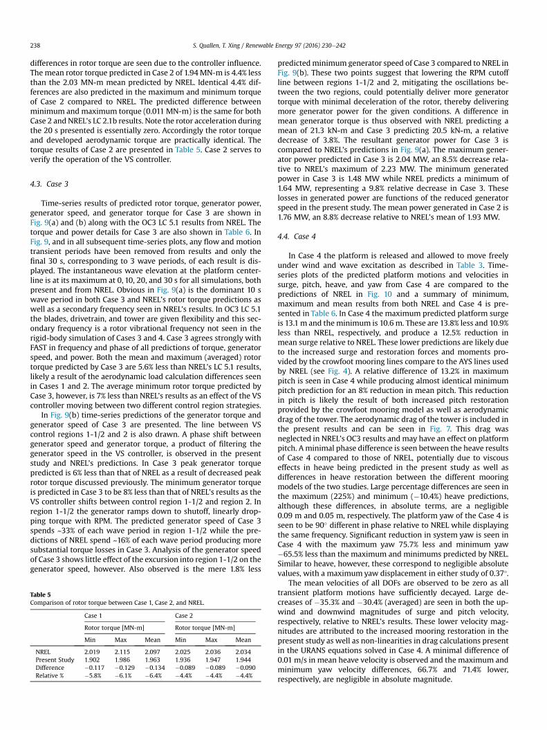
Time-series results of predicted rotor torque, generator power,generator speed, and generator torque for Case 3 are shown inFig. 9(a) and (b) along with the OC3 LC 5.1 results from NREL. Thetorque and power details for Case 3 are also shown in Table 6. InFig. 9, and in all subsequent time-series plots, any flow and motiontransient periods have been removed from results and only thefinal 30 s, corresponding to 3 wave periods, of each result is dis-played. The instantaneous wave elevation at the platform center-line is at its maximum at 0, 10, 20, and 30 s for all simulations, bothpresent and from NREL. Obvious in Fig. 9(a) is the dominant 10 swave period in both Case 3 and NREL’s rotor torque predictions aswell as a secondary frequency seen in NREL’s results. In OC3 LC 5.1the blades, drivetrain, and tower are given flexibility and this sec-ondary frequency is a rotor vibrational frequency not seen in therigid-body simulation of Cases 3 and 4. Case 3 agrees strongly withFAST in frequency and phase of all predictions of torque, generatorspeed, and power. Both the mean and maximum (averaged) rotortorque predicted by Case 3 are 5.6% less than NREL’s LC 5.1 results,likely a result of the aerodynamic load calculation differences seenin Cases 1 and 2. The average minimum rotor torque predicted byCase 3, however, is 7% less than NREL’s results as an effect of the VScontroller moving between two different control region strategies.

In Fig. 9(b) time-series predictions of the generator torque andgenerator speed of Case 3 are presented. The line between VScontrol regions 1-1/2 and 2 is also drawn. A phase shift betweengenerator speed and generator torque, a product of filtering thegenerator speed in the VS controller, is observed in the presentstudy and NREL’s predictions. In Case 3 peak generator torquepredicted is 6% less than that of NREL as a result of decreased peakrotor torque discussed previously. The minimum generator torqueis predicted in Case 3 to be 8% less than that of NREL’s results as theVS controller shifts between control region 1-1/2 and region 2. Inregion 1-1/2 the generator ramps down to shutoff, linearly drop-ping torque with RPM. The predicted generator speed of Case 3spends ~33% of each wave period in region 1-1/2 while the pre-dictions of NREL spend ~16% of each wave period producing moresubstantial torque losses in Case 3. Analysis of the generator speedof Case 3 shows little effect of the excursion into region 1-1/2 on thegenerator speed, however. Also observed is the mere 1.8% less

Table 5Comparison of rotor torque between Case 1, Case 2, and NREL.

Case 1 Case 2

Rotor torque [MN-m] Rotor torque [MN-m]

Min Max Mean Min Max Mean

NREL 2.019 2.115 2.097 2.025 2.036 2.034Present Study 1.902 1.986 1.963 1.936 1.947 1.944Difference �0.117 �0.129 �0.134 �0.089 �0.089 �0.090Relative % �5.8% �6.1% �6.4% �4.4% �4.4% �4.4%

predictedminimum generator speed of Case 3 compared to NREL inFig. 9(b). These two points suggest that lowering the RPM cutoffline between regions 1-1/2 and 2, mitigating the oscillations be-tween the two regions, could potentially deliver more generatortorque with minimal deceleration of the rotor, thereby deliveringmore generator power for the given conditions. A difference inmean generator torque is thus observed with NREL predicting amean of 21.3 kN-m and Case 3 predicting 20.5 kN-m, a relativedecrease of 3.8%. The resultant generator power for Case 3 iscompared to NREL’s predictions in Fig. 9(a). The maximum gener-ator power predicted in Case 3 is 2.04 MW, an 8.5% decrease rela-tive to NREL’s maximum of 2.23 MW. The minimum generatedpower in Case 3 is 1.48 MW while NREL predicts a minimum of1.64 MW, representing a 9.8% relative decrease in Case 3. Theselosses in generated power are functions of the reduced generatorspeed in the present study. The mean power generated in Case 2 is1.76 MW, an 8.8% decrease relative to NREL’s mean of 1.93 MW.

4.4. Case 4

In Case 4 the platform is released and allowed to move freelyunder wind and wave excitation as described in Table 3. Time-series plots of the predicted platform motions and velocities insurge, pitch, heave, and yaw from Case 4 are compared to thepredictions of NREL in Fig. 10 and a summary of minimum,maximum and mean results from both NREL and Case 4 is pre-sented in Table 6. In Case 4 the maximum predicted platform surgeis 13.1m and theminimum is 10.6 m. These are 13.8% less and 10.9%less than NREL, respectively, and produce a 12.5% reduction inmean surge relative to NREL. These lower predictions are likely dueto the increased surge and restoration forces and moments pro-vided by the crowfoot mooring lines compare to the AYS lines usedby NREL (see Fig. 4). A relative difference of 13.2% in maximumpitch is seen in Case 4 while producing almost identical minimumpitch prediction for an 8% reduction in mean pitch. This reductionin pitch is likely the result of both increased pitch restorationprovided by the crowfoot mooring model as well as aerodynamicdrag of the tower. The aerodynamic drag of the tower is included inthe present results and can be seen in Fig. 7. This drag wasneglected in NREL’s OC3 results and may have an effect on platformpitch. Aminimal phase difference is seen between the heave resultsof Case 4 compared to those of NREL, potentially due to viscouseffects in heave being predicted in the present study as well asdifferences in heave restoration between the different mooringmodels of the two studies. Large percentage differences are seen inthe maximum (225%) and minimum (�10.4%) heave predictions,although these differences, in absolute terms, are a negligible0.09 m and 0.05 m, respectively. The platform yaw of the Case 4 isseen to be 90� different in phase relative to NREL while displayingthe same frequency. Significant reduction in system yaw is seen inCase 4 with the maximum yaw 75.7% less and minimum yaw�65.5% less than the maximum and minimums predicted by NREL.Similar to heave, however, these correspond to negligible absolutevalues, with a maximum yaw displacement in either study of 0.37�.

The mean velocities of all DOFs are observed to be zero as alltransient platform motions have sufficiently decayed. Large de-creases of �35.3% and �30.4% (averaged) are seen in both the up-wind and downwind magnitudes of surge and pitch velocity,respectively, relative to NREL’s results. These lower velocity mag-nitudes are attributed to the increased mooring restoration in thepresent study as well as non-linearities in drag calculations presentin the URANS equations solved in Case 4. A minimal difference of0.01 m/s in mean heave velocity is observed and the maximum andminimum yaw velocity differences, 66.7% and 71.4% lower,respectively, are negligible in absolute magnitude.

Fig. 9. Comparisons of rotor torque and generator predictions between Case 3 and NREL-FAST.

Table 6Comparison of motions and power characteristics between Case 3, Case 4, and NREL.

Rotor torque [MN-m] Generator speed [RPM] Generator torque [kN-m] Generator power [MW]

Min Max Mean Min Max Mean Min Max Mean Min Max Mean

NREL 1.851 2.298 2.070 865 962 913 19.2 23.5 21.3 1.64 2.23 1.93Case 3 1.721 2.170 1.954 849 934 893 17.6 22.2 20.5 1.48 2.04 1.76Difference �0.130 �0.128 �0.115 �16 �28 �20 �1.6 �1.3 �0.8 �0.16 �0.19 �0.17% Relative to NREL �7.0% �5.6% �5.6% �1.8% �2.9% �2.2% �8.3% �5.5% �3.8% �9.8% �8.5% �8.8%

Surge [m] Pitch [�] Heave [m] Yaw [�]

Min Max Mean Min Max Mean Min Max Mean Min Max Mean

NREL 11.9 15.2 13.6 1.93 3.57 2.75 �0.48 0.04 �0.22 �0.37 0.29 �0.03Case 4 10.6 13.1 11.9 1.95 3.10 2.53 �0.43 0.13 �0.15 �0.09 0.10 0.01Difference �1.3 �2.1 �1.7 0.02 �0.47 �0.22 0.05 0.09 0.07 0.28 �0.19 0.04% Relative to NREL �10.9% �13.8% �12.5% 1.0% �13.2% �8.0% �10.4% 225.0% �31.8% �75.7% �65.5% �133.3%

Surge velocity [m/s] Pitch velocity [�/s] Heave velocity [m/s] Yaw velocity [�/s]

Min Max Mean Min Max Mean Min Max Mean Min Max Mean

NREL �0.98 0.98 0.00 �0.51 0.51 0.00 �0.16 0.16 0.00 �0.21 0.21 0.00Case 4 �0.66 0.66 0.00 �0.36 0.35 0.00 �0.17 0.17 0.00 �0.06 0.07 0.00Difference 0.32 �0.32 0.00 0.15 �0.16 0.00 �0.01 0.01 0.00 0.15 �0.14 0.00% Relative to NREL �32.7% �32.7% 0.0% �29.4% �31.4% 0.0% 6.3% 6.3% 0.0% �71.4% �66.7% 0.0%

Rotor torque [MN-m] Generator speed [RPM] Generator torque [kN-m] Generator power [MW]

Min Max Mean Min Max Mean Min Max Mean Min Max Mean

NREL 1.851 2.298 2.070 865 962 913 19.2 23.5 21.3 1.64 2.23 1.93Case 4 1.795 2.093 1.949 857 919 888 18.3 21.5 20.1 1.55 1.95 1.77Difference �0.056 �0.205 �0.121 �8 �43 �25 �0.9 �2.0 �1.2 �0.09 �0.28 �0.16% Relative to NREL �3.0% �8.9% �5.8% �0.9% �4.5% �2.7% �4.7% �8.5% �5.6% �5.5% �12.6% �8.3%

S. Quallen, T. Xing / Renewable Energy 97 (2016) 230e242 239

The time-series predictions of torque and power from Case 4alongwith NREL’s results, which are identical to those from Fig. 9(a)but repeated for comparison, are shown in Fig. 11(a) and (b).Comparedwith Case 3, which used NREL’s exact OC3 LC 5.1motionsand show relatively consistent differences from NREL in rotor tor-que, the platform motions of Case 4 are controlled by the crowfootmooring model and are subjected to lower magnitudes in surgingand pitching velocities (see Fig.10(a) and (b) and Table 6). Themeanrotor torque predicted in Case 4, 1.949 MN-m, is 5.8% less than themean rotor torque predicted by NREL in LC 5.1. This is very similarto the 5.6% decrease of Case 3 and is on the order of the meandifferences seen in Cases 1 and 2, attributable to reduced calculatedaerodynamic loading. However the maximum rotor torque pre-dicted in Case 4 is predicted to be 8.9% less than that of NREL, and isobserved to only deviate 0.144 MN-m, 7.4% relative to its mean,while NREL predicts a deviation of 0.228 MN-m, 11.0% relative to

their mean. The minimum rotor torque in Case 4 is predicted to be3.0% less than that of NREL and to deviate 0.154MN-m, 7.9% relativeto its mean, while NREL predicts a deviation of 0.219 MN-m, 10.6%relative to their mean. In Fig. 11(a) Case 4 clearly shows less devi-ation from the mean in both maximum and minimum rotor torque.This difference is attributed to the decreased upwind and down-wind velocities of Case 4 relative to NREL due to increased resto-ration forces of the crowfoot mooring model. The difference inmaximum developed torque may also be a result of predictedseparation caused by the increased effective angle of attack (AoA)experienced during the upwind velocity phase of platform motion.Upwind relative velocity of the platform increases the effective AoAseen by the blade by increasing the magnitude of the incomingwind velocity component, nominally perpendicular to the rotorplane. This in turn generates high magnitude pressure coefficientsat the leading edge of the blade but develops strong adverse

Fig. 10. Comparison of platform motions between Case 4 and NREL-FAST.

Fig. 11. Comparisons of aerodynamic torque and generator predictions between Case 4 and NREL-FAST.

S. Quallen, T. Xing / Renewable Energy 97 (2016) 230e242240

pressure gradients at the rear, promoting separation. The full spanof the suction side of the blade during both maximum downstreamand maximum upstream velocities is shown Fig. 12(a) and (b),respectively, contoured by local CP. The developed suction pressureis shown to be significantly lower in magnitude during maximumdownstream velocity (Fig. 12(a)) than during maximum upstreamvelocity (Fig. 12(b)) along the entire blade span beyond the roottransition region. In both situations a large separation region existsat the TE of the cylindrical root and the transition region betweencylinder and blade, as well as similar separation regions at the bladetip. The maximum downstream situation remains attached overthe remainder of the span of the blade. In the maximum upstream

situation, however, the root separation region spans 7% more of theblade and TE separation occurs on the outboard 1/3 of the blade,including a large-scale separation bubble at 82% span. In Fig. 13 theoutboard 20% of blade 1 is shown during maximum downstreamvelocity in the left frame (a) and during maximum upstream ve-locity in the right frame (b). The TE separation of the upstreamvelocity situation is more clearly visualized in Fig. 13(b), along withthe separation bubble detailed in the inset. The increased AoAduring maximum upstream velocity can be seen in the plane-section streamlines of Fig. 13(b) compared to those of Fig. 13(a),as well as the increased CP magnitudes on both the suction andpressure sides of the blade. While producing similar mean values,

Fig. 13. Outboard 20% of blade showing limiting streamlines and colored by CP: (a)maximum downstream platform velocity; (b) maximum upstream velocity. Insetshows separation zone at 82% blade span.

S. Quallen, T. Xing / Renewable Energy 97 (2016) 230e242 241

the smaller deviations of rotor torque produce smaller bendingmoments on the blades and less torsion in the shafts, potentiallyreducing overall fatigue. This adds to the importance of themooring system to limit streamwise velocity fluctuations.

The generator speed predicted in Case 4 is shown in Fig. 11(b).The diminished platformvelocities in Case 4 are observed to reducedeviations from themean generator speed compared to that of Case2, and the generator spends only 28% of the wave period in VScontrol region 1-1/2 instead of the 33% observed in Case 2. Themaximum generator torque of Case 4, also shown in Fig. 11(b),deviates 1.4 kN-m from amean of 20.1 kN-m (7.0% relative) and theminimum generator torque deviates 1.8 kN-m from the mean (9.0%relative). These same generator torque deviations are observed inCase 3, perhaps more directly comparable to Case 4 than NREL’sresults due to solution modeling differences between the presentstudy and NREL’s FAST software. In Case 3 is predicted a 1.7 kN-mdeviation from the mean in maximum generator torque (8.4%relative) and a substantial 2.9 kN-m deviation in minimum gener-ator torque (14.2% relative). The lesser deviations of generatortorque in Case 4 compared to Case 3 help to reduce fatigue alongthe entire drivetrain. The resultant generator power developed inCase 4 is shown in Fig. 11(a). The maximum power generated inCase 4 is 1.95 MW, which is 12.6% less than the maximum of2.23 MW generated by NREL and 4.4% less than the 2.04 MWmaximum generated in Case 3. The minimum power generated inCase 4 is 1.55 MW, which is 5.5% less than the minimum 1.64 MWpredicted by NREL and 4.5% greater than the 1.48 MW minimumpredicted in Case 3. The difference between the minimum gener-ator power in Case 4 and Case 3 is largely a function of the smalleramount of time spent in VS control region 1-1/2 in Case 4 comparedto Case 3. The mean power generated in Case 4 is 1.77 MW, which is8.3% less than the predicted mean power by NREL. The meangenerated power of Case 4 is 0.01 MW higher than that of Case 3.While this difference is relatively negligible it suggests that mini-mizing platform velocities, thereby reducing generator speed de-viation, can help with more precise controller design.

5. Conclusions

An inertial rotor model with a VS generator-torque controller iscoupled with high resolution CFD and a mooring force model topredict motion and generated power of FOWT. The developed codeis utilized in four simulations of the OC3-Hywind FOWT using theOC3’s LC 2.1a, 2.1b, and 5.1 wind and wave conditions. Results arecompared to the publically available OC3 results of NREL using theirFAST software. Simulations utilize an incremental approach forverification of the method. OC3 LC 2.1a, featuring a fixed platformand rotor rotational velocity, is first simulated (Case 1) to determinea baseline expectation of rotor torque considering the differentaerodynamic solution differences between the present CFD solver

Fig. 12. Limiting streamlines on suction side of blade, colored by CP: (a) max

and NREL’s FAST. The results show about 6% less maximum, mini-mum, and mean rotor torque than NREL’s predictions, within therange of OC3 participants.

A second simulation (Case 2) is performed using the conditionsof OC3 LC 2.1b. The platform is still fixed, however the inertial rotormodel and VS controller are now activated to investigate the effectof torque control on rotor torque. A very consistent difference of4.4% is seen between Case 2 and NREL’s results in each of mean,maximum, and minimum rotor torque, verifying the operation ofthe VS controller.

NREL’s OC3 LC 5.1 predicted platform motions are prescribed ina simulation (Case 3) while using the inertial rotor model and VScontroller. The results of Case 3 serve to identify the effect of theunsteady aerodynamic solution differences between CFD and FASTon generator torque and power predictions. The generator speedresults of Case 3 agree within to 3% of NREL’s generator speedpredictions. However the generator speed of Case 3 is observed tospend 17% more time per wave period in a lower VS control regionthan NREL’s speed, and minimum generator torque predictions ofCase 3 are observed to be 8.3% lower than those of NREL as a result.Mean generated power is predicted 8.8% below the mean of NREL’spredicted power due to the decreases in generator speed, andcorresponding generator torque, experienced during the extra timespent in the lower control region. The results of Case 3 suggest arecalibration of the VS control region cutoffs to help keep generatorspeed up and increase overall generator power developed.

A final simulation (Case 4) is performed where the platform

imum downstream platform velocity; (b) maximum upstream velocity.

S. Quallen, T. Xing / Renewable Energy 97 (2016) 230e242242

motions are predicted using semi-coupled 2-phase CFD and acrowfoot mooring model. The inertial rotor model and VScontroller are active and both aerodynamic and hydrodynamicloading are considered. Reductions in mean surge translation andmean pitch relative to NREL’s predictions are observed due toincreased mooring forces. A 32.7% reduction in maximum platformsurging velocity and a 31.4% reduction in maximum platformpitching velocity are also observed. These correspond to reducedupstream and downstream velocities and are shown to keep thegenerator speed in a more favorable VS control region, and gener-ated power is slightly increased (0.01 MW) from Case 3 despite a0.2% reduction in mean rotor torque. This again demonstrates theimportance of VS control region calibration. Separation over theoutboard 1/3 of the blade is predicted during maximum upstreampitching velocity, verifying the importance of stabilization of theplatform.

6. Future work

The present results suggest a modification of the VS controllerscheme. The VS controller is designed to maximize power capturebelow rated rotor rotational speed. At, or beyond rated velocity,however, requires a method of releasing torque from the system toavoid generator overload. A blade-pitch controller will be added inthe future to the developed code for analysis of rated conditionsand beyond. Combined with the Mann wind model, recentlyimplemented into CFDShip-Iowa [38] OC3 LC 5.2 will be run. Thecrowfoot mooring lines, seen to add stability in the present study,could potentially be optimized, including clump weights and pre-dicted dynamics. Quantitative verification and validation should beperformed to evaluate the numerical and modeling errors anduncertainties using the recent general framework for LES [39]. Thepotential for incorporation of other models into the present systemalso exist. These potential modifications could include a drivetraindynamic model or deformable blades and tower, both investigatedin Ref. [19], or brakes for start-up and shut-down simulations.

Acknowledgements

The present study is funded by the National Science Foundation,Division of Chemical Bioengineering, Environmental, and TransportSystems, under award number 1066873. All simulations presentedwere performed using the Idaho National Laboratory’s Falcon HPC,an SGI ICE with 16,416 cores. Gratitude is offered to both of theseorganizations for their help and resources. NREL’s accomplish-ments in all phases of the OC3, several of which are compared to inthis study, are also acknowledged. Jason Jonkman of NREL isthanked for personally answering questions and clarifying OC3results.

References

[1] D. Wind, Block Island Wind Farm e Deepwater Wind, 2015 at: http://dwwind.com/project/block-island-wind-farm/.

[2] DOE, Wind Vision: a New Era for Wind Power in the United States, 2015.[3] M. Schwartz, D. Heimiller, S. Haymes, W. Musial, Assessment of Offshore Wind

Energy Resources for the United States, 2010.[4] W. Musial, B. Ram, Large-scale Offshore Wind Power in the United States:

Assessment of Opportunities and Barriers, 2010.[5] T. Burton, Wind Energy Handbook, Wiley, Chichester, West Sussex, 2011.[6] J.R. Morison, J.W. Johnson, S.A. Schaaf, The force exerted by surface waves on

piles, J. Pet. Technol. 2 (1950) 149e154.[7] J.M. Jonkman, M.L. Buhl, FAST User’s Guide, 2005.[8] D. Matha, S.-A. Fischer, S. Hauptmann, P.W. Cheng, D. Bekiropoulos, T. Lutz,

T. Duarte, K. Boorsma, Variations in ultimate load predictions for floatingoffshore wind turbine extreme pitching motions applying different aero-dynamic methodologies, in: ISOPE-2013, International Society of Offshore andPolar Engineers, Anchorage, AK, 2013.

[9] T. Sebastian, M. Lackner, A comparison of first-order aerodynamic analysismethods for floating wind turbines, in: 48th AIAA Aerospace Sciences MeetingIncluding the New Horizons Forum and Aerospace Exposition, AmericanInstitute of Aeronautics and Astronautics, 2010.

[10] C. Bak, H. Aagaard-Madsen, J. Johansen, Influence from blade-tower interac-tion on fatigue loads and dynamics, in: A. Zervos (Ed.), Proc Wind Energy forthe New Millennium Conference, München, 2001, pp. 394e397.

[11] S. Quallen, T. Xing, An investigation of the blade tower interaction of a floatingoffshore wind turbine, in: ISOPE-2015, Kona, Big Island, Hawaii, 2015, pp. 8.

[12] D. Matha, M. Schlipf, A. Cordle, R. Pereira, J. Jonkman, Challenges in Simulationof Aerodynamics, Hydrodynamics, and Mooring-line Dynamics of FloatingOffshore Wind Turbines, NREL, 2011.

[13] J.L. Steger, J.A. Benek, On the use of composite grid schemes in computationalaerodynamics, Comput. Methods Appl. Mech. Eng. 64 (1987) 301e320.

[14] A. S�anchez-Caja, P. Rautaheimo, T. Siikonen, Computation of the incom-pressible viscous flow around a tractor thruster using a sliding-mesh tech-nique, in: Proceedings of the 7th International Conference on Numerical ShipHydrodynamics, 1999, pp. 19e21. Nantes, France.

[15] NREL, Unsteady Aerodynamics Experiment Phase VI Wind Tunnel Test Con-figurations and Available Data Campaigns, NREL, 2001.

[16] Y. Li, K.J. Paik, T. Xing, P.M. Carrica, Dynamic overset CFD simulations of windturbine aerodynamics, Renew. Energy 37 (2012) 285e298.

[17] F. Zahle, N.N. Sørensen, J. Johansen, Wind turbine rotor-tower interactionusing an incompressible overset grid method, Wind Energy 12 (2009)594e619.

[18] T.-T. Tran, D.-H. Kim, The platform pitching motion of floating offshore windturbine: a preliminary unsteady aerodynamic analysis, J. Wind Eng. Ind.Aerodyn. 142 (2015) 65e81.

[19] Y. Li, in: Coupled Computational Fluid Dynamics/Multibody Dynamics Methodwith Application to Wind Turbine Simulations, Mech. Eng., University of Iowa,2014.

[20] S. Quallen, T. Xing, P. Carrica, Y. Li, J. Xu, CFD Simulation of a floating offshorewind turbine system using a quasi-static crowfoot mooring-line model,J. Wind Energy 1 (2014) 143e152.

[21] J. Jonkman, Definition of the Floating System for Phase IV of OC3, NREL, 2010.[22] J. Jonkman, S. Butterfield, W. Musial, G. Scott, Definition of a 5-MW Reference

Wind Turbine for Offshore System Development, NREL, 2009.[23] J. Jonkman, T. Larsen, A. Hansen, T. Nygaard, K. Maus, M. Karimirad, Z.M. Gao,

T. Moan, T.I. Fylling, J. Nichols, M. Kohlmeier, J. Vergara, D. Merino, W. Shi,H. Park, Offshore code comparison collaboration within IEA wind task 23:phase IV results regarding floating wind turbine modeling, in: European WindEnergy Conference (EWEC), NREL, Warsaw, Poland, 2010.

[24] Statoil, Hywind by Statoil: the Floating Wind Turbine, 2012 at: http://www.statoil.com/en/TechnologyInnovation/NewEnergy/RenewablePowerProduction/Offshore/Hywind/Downloads/Hywind_nov_2012.pdf.

[25] J. Huang, P. Carrica, F. Stern, Semi-coupled air/water immersed boundaryapproach for curvilinear dynamic overset grids with application to ship hy-drodynamics, Int. J. Numer. Methods Fluids 58 (2008) 591e624.

[26] P.M. Carrica, R.V. Wilson, F. Stern, An unsteady single-phase level set methodfor viscous free surface flows, Int. J. Numer. Methods Fluids 53 (2007)229e256.

[27] P.M. Carrica, R.V. Wilson, R.W. Noack, F. Stern, Ship motions using single-phase level set with dynamic overset grids, Comput. Fluids 36 (2007)1415e1433.

[28] R. Noack, SUGGAR: a general capability for moving body overset grid as-sembly, in: 17th AIAA Computational Fluid Dynamics Conference, AIAA,Toronto, Ontario, Canada, 2005.

[29] T. Xing, P. Carrica, F. Stern, Computational towing tank procedures for singlerun curves of resistance and propulsion, J. Fluids Eng. 130 (2008)1011021e10110214.

[30] P. Spalart, S. Deck, M. Shur, K. Squires, M. Strelets, A. Travin, A new version ofdetached-eddy simulation, resistant to ambiguous grid densities, Theor.Comput. Fluid Dyn. 20 (2006) 181e195.

[31] T. Xing, P. Carrica, F. Stern, Large-scale RANS and DDES computations ofKVLCC2 at drift angle 0 degree, in: Gothenburg 2010: a Workshop on CFD inShip Hydrodynamics, 2010. Gothenburg, Sweden.

[32] F. Menter, Two-equation eddy-viscosity turbulence models for engineeringapplications, AIAA J. 32 (1994) 1598e1605.

[33] S.W. Smith, The Scientist and Engineer’s Guide to Digital Signal Processing,California Techn. Publ., San Diego Calif., 1997.

[34] P. Passon, M. Kühn, S. Butterfield, J. Jonkman, T. Camp, T.J. Larsen, OC3benchmark exercise of aero-elastic offshore wind turbine codes, J. Phys. Conf.Ser. 75 (2007).

[35] F.M. White, Fluid Mechanics, McGraw-Hill Higher Education, Boston, 2008.[36] J.C.R. Hunt, A.A. Wray, P. Moin, Eddies, Stream, and Convergence Zones in

Turbulent Flows, Report CTR-S88, C.F.T. Research, 1988.[37] J. Jonkman, W. Musial, Offshore Code Comparison Collaboration (OC3) for IEA

Task 23 Offshore Wind Technology and Deployment, 2010.[38] Y. Li, A.M. Castro, P.M. Carrica, T. Sinokrot, W. Prescott, Coupled multi-body

dynamics and CFD for wind turbine simulation including explicit wind tur-bulence, Renew. Energy 76 (2015) 338e361.

[39] T. Xing, A general framework for verification and validation of large eddysimulations, J. Hydrodyn. Ser. B 27 (2015) 163e175.