Cfd Post Ansys

ANSYS CFD-Post Tutorials

mailto:[email protected]

http://www.ansys.com/

Copyright and Trademark Information

Disclaimer Notice

U.S. Government Rights

Third-Party Software

Table of Contents

1. Introduction to the Tutorials

2. Post-processing Fluid Flow and Heat Transfer in a Mixing Elbow

3. Turbo Post-processing

4. Quantitative Post-processing

Chapter 1: Introduction to the Tutorials

Using Help

Help Contents

F1

Help Contents

Tip

Chapter 2: Post-processing Fluid Flow and Heat Transfer in a Mixing

Elbow

Problem Description

Note

Figure 2.1 Problem Specification

2.1. Create a Working Directory

Copying the CAS and DAT/CDAT Files

<CFXROOT>\examples <CFXROOT>

.cas .cdat elbow1.cas.gz

elbow1.cdat.gz elbow3.cas.gz elbow3.cdat.gz el-

bow_tracks.xml

cfd-post-elbow.zip

Download Software ANSYS

Download Center Wizard

http://www.ansys.com/customerportal/

Next Step

Current Release and Updates

Next Step

Next Step

ANSYS Documentation and Examples

ANSYS Fluid Dynamics Tutorial Inputs

Next Step

ANSYS Fluid Dynamics Tutorial Inputs ANSYS_Fluid_Dy-

namics_Tutorial_Inputs.zip

.zip

v140\Tutorial_Inputs\Flu-

id_Dynamics\<product>

elbow1.cas.gz elbow1.dat.gz elbow3.cas.gz

elbow3.dat.gz elbow_tracks.xml cfd-post-elbow.zip

2.2. Launch CFD-Post

Start All Programs > ANSYS 14.0 > Fluid Dynamics > CFD-Post

14.0 Properties

Start in OK

All Programs > ANSYS 14.0 > Fluid Dynamics > CFD-Post 14.0

cfdpost.exe

Start All Programs > ANSYS 14.0 > Fluid Dynamics > CFX 14.0

cfx5launch

cfx5launch

cfx5launch

Working Directory

CFD-Post 14.0

ANSYS Workbench

File Save As

Component Systems Results

Project Schematic

Results Edit CFD-Post

FLUENT

3D Dimension

Processing Option Serial

Display Mesh After Reading Embed Graphics Windows

Double-Precision

Tip

Default

cfd-post-elbow.zip

Show More Options

Working Directory

Working Directory

Browse For Folder

OK

File Read Case & Data elbow1.cas.gz

File Export to CFD-Post

Select Quantities

Write

File Read Case & Data elbow3.cas.gz

Export to CFD-Post Open CFD-Post Write

OK

2.3. Display the Solution in CFD-Post

lengthAve

Prepare the Case and Set the Viewer Options

elbow1.cdat.gz File Load

Results Load Results File elbow1.cdat.gz Open

OK

User Location and Plots Wireframe Outline

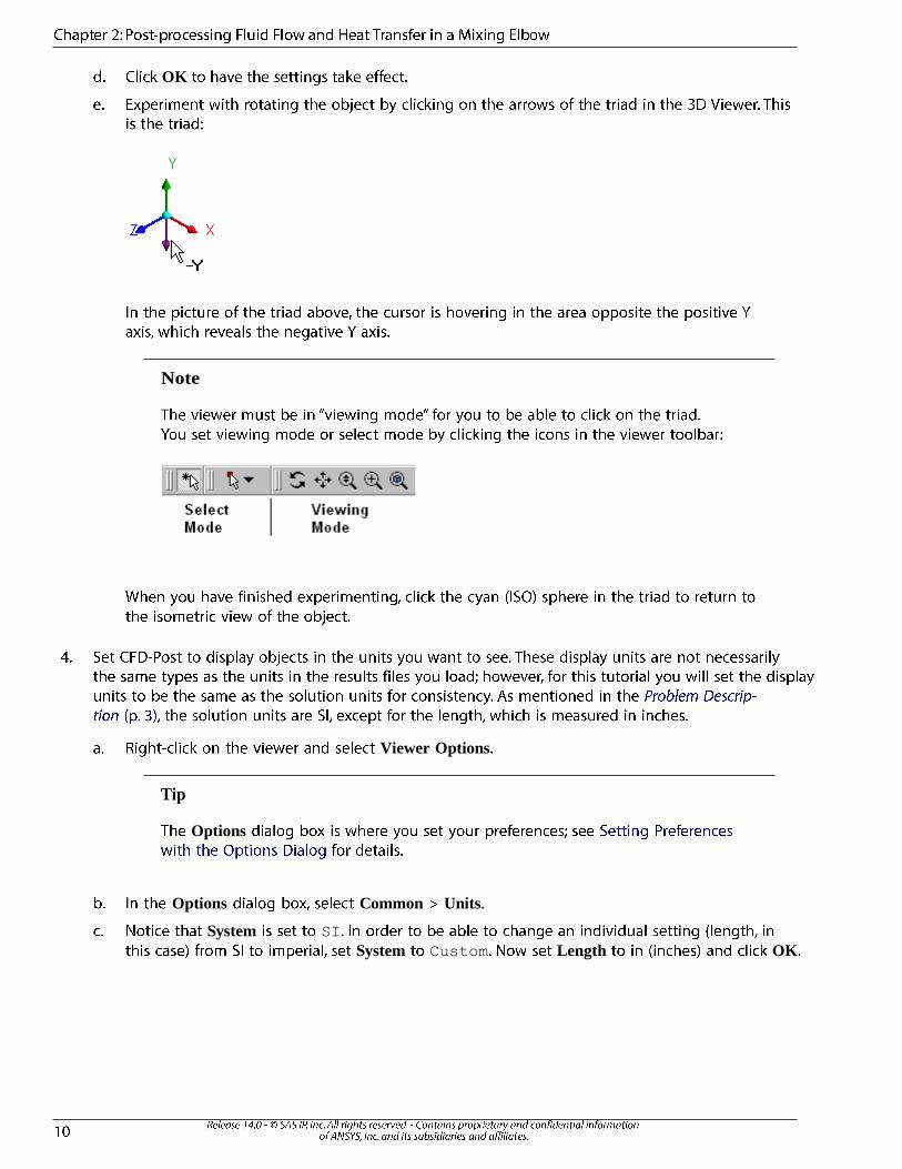
Viewer Options

Options CFD-Post Viewer

Background Color Type

Background Color Color

Color

Text Color

Edge Color

OK

Note

Viewer Options

Tip

Options

Options Common Units

System SI

System Custom Length OK

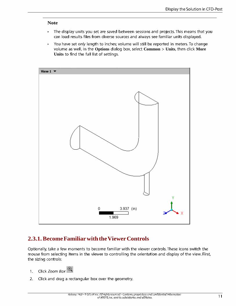
Note

Options Common Units More

Units

2.3.1. Become Familiar with the Viewer Controls

Figure 2.2 Orientation Control Cursor Types

Tip

Predefined Camera View From -X

Predefined Camera Isometric View (Z Up)

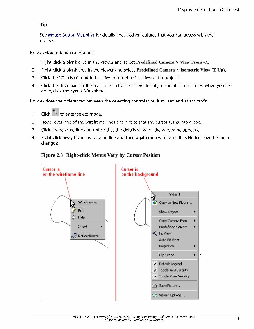
Figure 2.3 Right-click Menus Vary by Cursor Position

Outline elbow1 fluid wall

Outline elbow1 fluid wall

2.3.2. Create an Instance Reflection

Reflect/Mirror

Tip

2.3.3. Show Velocity on the Symmetry Plane

Insert Contour Insert Contour

OK

Tab Setting Value

Locations

Apply

Ctrl

Render

Lighting Apply

Z

Figure 2.4 Velocity on the Symmetry Plane

Render Show Contour Lines

Constant Coloring

Color Mode User Specified Line Color

Line Color

Apply

Figure 2.5 Velocity on the Symmetry Plane (Enhanced Contrast)

User Locations and Plots Contour 1

Outline

Tip

Outline

Hide

2.3.4. Show Flow Distribution in the Elbow

Insert Vector

OK

Geometry Domains fluid Locations symmetry

Apply

Symbol Symbol Size 4

Apply

Figure 2.6 Vector Plot of Velocity

Color

Mode Variable Variable

Variable Temperature

Apply

Symbol

Symbol Arrow3D Apply

Hide

Variable Geometry

Variable

Color

Insert Streamline OK

Start From

Location Selector

Location Selector Ctrl velocity inlet 5

velocity inlet 6 OK

Preview Seed Points

Geometry Variable Velocity

Color

Mode Variable Variable

Variable Turbulence Kinetic Energy

Range Local

Apply

Figure 2.7 Streamlines of Turbulence Kinetic Energy

Streamline 1 Outline Delete

Streamline 1

Vector 1 Streamline

1 Outline

2.3.5. Show the Vortex Structure

Outline

User Locations and Plots Wireframe

Cases elbow1 fluid wall

wall

Render Transparency 0.75

Apply

Insert Location Vortex Core Region OK

Vortex Core Region 1 Geometry Method Absolute

Helicity Level .01

Render Transparency 0.2 Apply

Color Color Apply

Predefined Camera Isometric View (Y up)

Outline Streamline 1

Figure 2.8 Absolute Helicity Vortex

wall Streamline 1 Vortex Core Region 1

Wireframe

2.3.6. Show Volume Rendering

Insert Volume Rendering OK

Volume Rendering 1 Geometry Variable Temperature

Color Mode Variable Variable Temperature Apply

Predefined

Camera Isometric View (Y up)

Figure 2.9 Volume Rendering of Temperature

2.3.7. Compare a Contour Plot to the Display of a Variable on a Boundary

Predefined Camera View From -Y

Outline pressure outlet 7 elbow1 fluid

View 1

Color

Mode Variable

Variable Pressure

Range Local

Apply

View 2

Outline fluid pressure outlet 7

Insert Contour

OK

Locations pressure outlet 7

Variable Pressure

Range Local

Apply

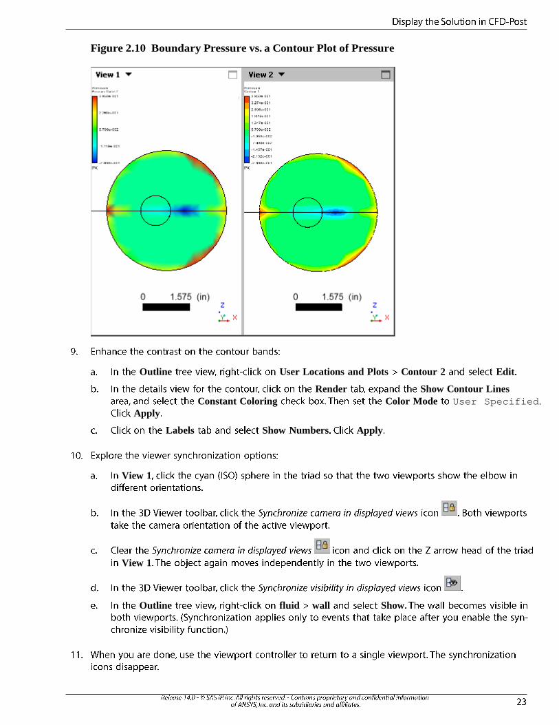
Figure 2.10 Boundary Pressure vs. a Contour Plot of Pressure

Outline User Locations and Plots Contour 2 Edit

Render Show Contour Lines

Constant Coloring Color Mode User Specified

Apply

Labels Show Numbers Apply

View 1

View 1

Outline fluid wall Show

2.3.8. Review and Modify a Report

Report Viewer

Report Viewer

Outline Report Title Page Title Content

Details of Report Title Page Analysis of Heat Transfer in a Mixing

Elbow

Apply Refresh Preview Report Viewer

Outline User Location and Plots Contour 1 Default Legend

View 1 Wireframe Contour 1 Geometry Variable

Temperature Apply

Insert Figure Insert Figure

OK

Outline Report Figure 1 Caption Temperature

on the Symmetry Plane Apply

Report Viewer

Report Viewer Refresh

Publish Publish Report

OK Report.htm

Outline Hide All Wireframe

Tip

2.3.9. Create a Custom Variable and Animate the Display

Expressions Expressions

New

New Expression DynamicHeadExp

OK

Definition

Density * abs(Velocity)^2 / 2

Density

abs abs

Velocity

Tip

Definition

Apply

Variables Variables

New

New Variable DynamicHeadVar

OK

Expression

DynamicHeadExp Apply

Insert YZ Plane

Color Variable Render Lighting

Apply

Animate Animation

Animation Close

Tip

Ctrl Animation

Figure 1 View

1

User Locations and Plots Hide All

Wireframe Default Legend View 1

2.3.10. Load and Compare the Results to Those in a Refined Mesh

File Load Results Load Results File

Load Results File Keep current cases loaded

elbow3.cdat.gz elbow3.cdat Open

View 1 elbow1

View 2 elbow3 Outline Cases elbow1 elbow3

Cases Case Comparison

Insert Contour

User Location and Plots

elbow3 Insert Contour

OK

Tab Set-

ting

Value

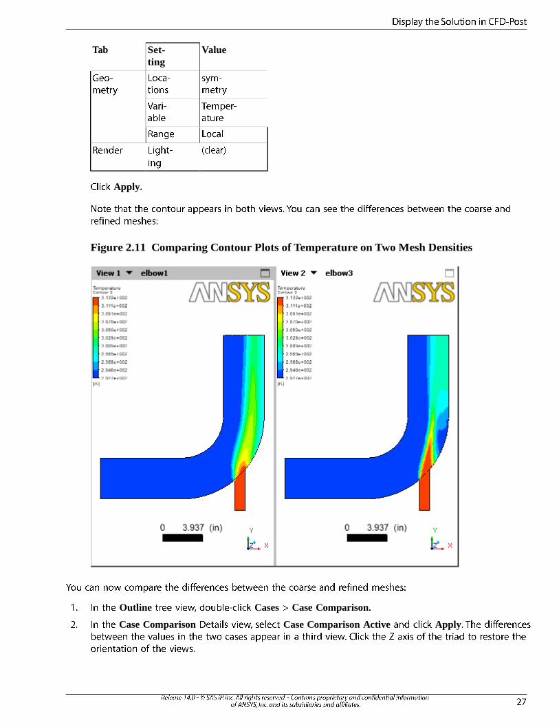
Apply

Figure 2.11 Comparing Contour Plots of Temperature on Two Mesh Densities

Outline Cases Case Comparison

Case Comparison Case Comparison Active Apply

Figure 2.12 Displaying Differences in Contour Plots of Temperature on Two Mesh

Densities

Difference Case Comparison Active Apply

Outline elbow3 Unload

2.3.11. Display Particle Tracks

Note

elbow_tracks.xml examples

elbow1.cdat elbow_tracks.xml

File Import Import FLUENT Particle Track File

Import FLUENT Particle Track File elbow_tracks.xml

Open

OK

Outline User Locations and Plots FLUENT PT for Anthracite

Injections

injection-0

Apply

injection-0,injection-1

Apply

Color

Mode Variable

Variable Anthracite.Injection

Apply

Geometry

Reduction Type Reduction Factor

Reduction 2

Apply

Reduction 1 Apply

Animate

Options

Options Symbol Size 2 Symbol Fish3D OK

Animations

An-

imation

Insert Vector

Insert Vector OK

Geometry

Locations

Reduction

Factor

Variable

Tip

Symbol Symbol Size

Apply

User locations and Plots FLUENT PT for Anthracite

Color

Mode Variable

Variable Anthracite.Particle Time

Apply

Geometry Injections injection-0

Apply

Symbol Show Track Numbers Apply

Filter

Track

Track 54

Apply

Insert Chart

Insert Chart Particle 54 OK

Chart Viewer

Title Particle Time vs. Particle Velocity

Data Series Series 1 Location FLUENT PT for Anthracite

X Axis Variable Anthracite.Particle Time

Y Axis Variable Anthracite.Particle Y Velocity

Apply

Y Axis Variable Pressure

General Title Particle Time vs. Pressure

Apply

lengthAve

Tools Function Calculator

Function Calculator Function lengthAve

Location FLUENT PT for Anthracite

Variable Pressure

Show equivalent expression

Calculate lengthAve(Pressure)@FLUENT PT for Anthracite

2.4. Save Your Work

.cst

File Save State

.cst .can .cas.gz .cd-

at.gz

Warning Yes

File Close Ctrl W File Load State

File Quit

Project Schematic Results

Outline Contour 1

Save Picture

Save casename

Tip

Save Picture

Outline Contour 1 FLUENT PT for Anthracite Plane 1

Animate Animation

Repeat Repeat

Save Movie

Close Animation

File Quit

2.5. Generated Files

elbow1.cst elbow1.can

elbow1.wmv

elbow1.png

Report.htm

Chapter 3: Turbo Post-processing

3.1. Problem Description



Copying the Sample Files

<CFXROOT>/examples <CFXROOT>

turbo.cdat.gz turbo.cas.gz

cfd-post-turbo.zip




Next Step


Next Step

Next Step



Next Step



.zip



turbo.cas.gz turbo.dat.gz cfd-post-

turbo.zip

3.3. Launching CFD-Post

Start All Programs > ANSYS 14.0 > Fluid

Dynamics > CFD-Post 14.0 Properties Start

in OK All Programs > ANSYS 14.0 > Fluid Dynamics > CFD-Post 14.0

Start Start All Programs > ANSYS 14.0 > Fluid Dynam-

ics > CFX 14.0

cfx5launch

cfx

cfx5launch

Working Directory

CFD-Post 14.0

ANSYS Workbench

File Save As


Project Schematic


FLUENT

3D Dimension

Serial Processing Options

Display Mesh After Reading Embed Graphics Windows

Double-Precision

Tip

Default

cfd-post-turbo.zip

Show More Options

Working Directory

Working Directory

Browse For Folder

OK

File Read Case & Data turbo.cas.gz

File Export to CFD-Post

FLUENT Variables Required by Turbo Reports

Write

3.4. Displaying the Solution in CFD-Post

Prepare the Case and Set the Viewer Options

turbo.cdat.gz

File Load Results Load Results File turbo.cdat.gz

Open

OK

Wireframe

Wireframe Outline

Viewer Options

Tip

Options


System OK

Note

Wireframe Outline

Edge Angle Apply

Tip

Details of Wireframe

F1

Wireframe Defaults Apply

Viewer Options




Color

Text Color

Edge Color

OK

3.5. Initializing the Turbomachinery Components

Turbo Turbo

Turbo initialization No

Turbo Initialization fluid (fluid)

Definition Turbo Regions

Hub

Ctrl Location Selector wall diffuser hub wall hub

wall inlet hub

OK Hub

Shroud wall diffuser shroud wall

inlet shroud wall shroud

Blade wall blade

Inlet inlet

Outlet outlet

Periodic 1 periodic.33 periodic.34

periodic.35

periodic.*shadow periodic.*

Instancing

# of Copies 1

Axis Definition from File Method Principal Axis

Axis Z

# of Passages 20

Initialize

Tip

Initialization Turbo Initialization

Calculate Velocity Components

Turbo

3.6. Comparing the Blade-to-Blade, Meridional, and 3D Views

Turbo Three Views Initialization

Turbo Initialization View Blade to Blade View Meridi-

onal View

Blade to Blade View

Pressure

Blade to Blade View Edit

Blade-to-Blade Plot Plot Type Color Contour

Color Contour

Variable Velocity

# of Contours 21

Apply

Meridional View

Meridional View Edit

Meridional Plot Plot Type Color Contour

# of Contours 21

Apply

3.7. Displaying Contours on Meridional Isosurfaces

Tree Plots Single View

3D View

Insert Location Isosurface

Tab

Field

Value

(p. 52)

Footnote

Apply

Geometry

.2 .4 .6 .8 .99

Tip

Isosurface 1 Tree Duplicate

Geometry Value Apply

Note

Linear BA Streamwise Location

M Length Normalized

3.8. Displaying a 360-Degree View

Outline Hide All

User Locations and Plots Wireframe

Cases turbo fluid

Instancing # of Copies 20

Axis Definition from File Method Principal Axis Axis

Z

Apply

3.9. Calculating and Displaying Values of Variables

Function Calculator

Tools Function Calculator Calculators Function

Calculator

Function Calculator

Function massFlowAve

Location inlet

Variable Pressure

Function Calculator Show equivalent expression

Calculate

Function Calculator

Table Viewer

Table Viewer

Table Viewer New Table

Inlet and Outlet Values OK

Table Viewer Function CFD-Post massFlow

=massFlow()@

Location inlet

Enter

Location outlet

Function CFD-Post massFlowAve

Variable Pressure Location

inlet Enter

Location outlet

Shift

Shift

Report Viewer Refresh Report Viewer

Note

Table Viewer

Report Viewer Publish

3.10. Displaying the Inlet to Outlet Chart

Inlet to Outlet

Turbo Turbo Charts Inlet to Outlet

Apply

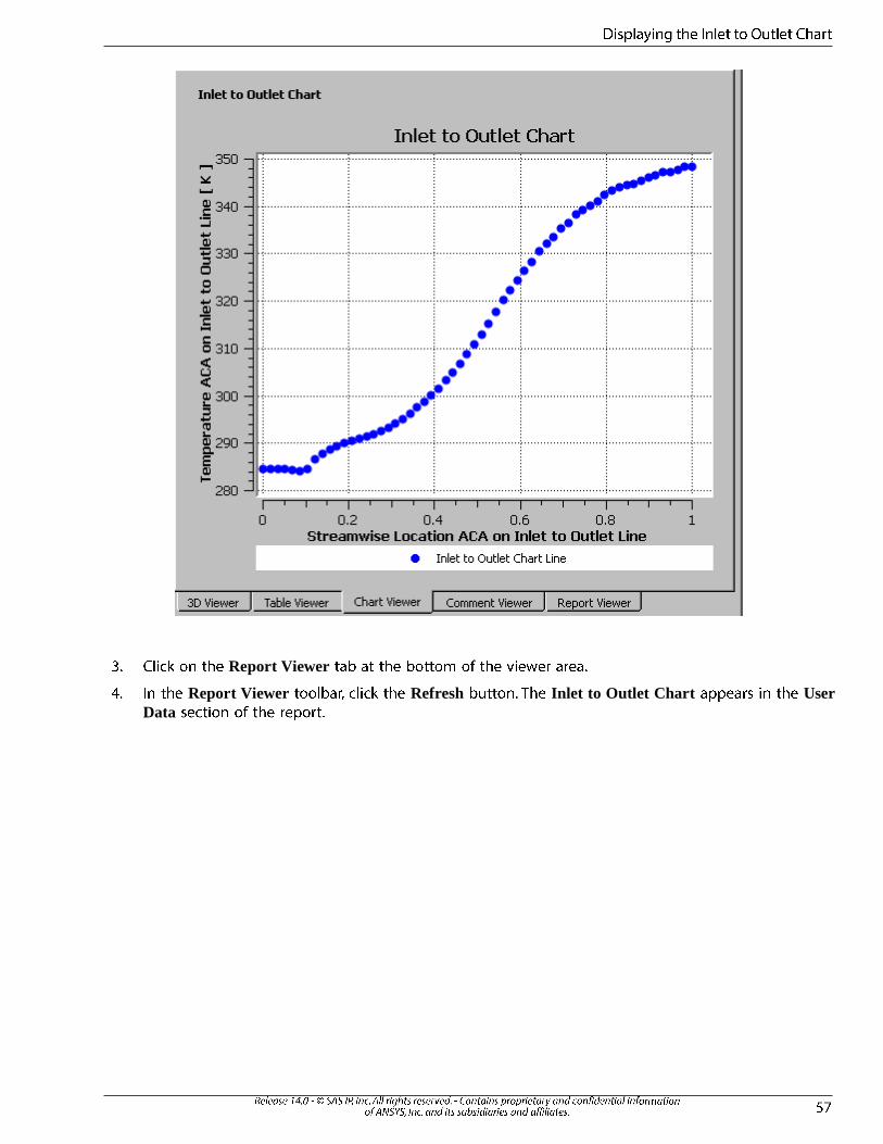
Report Viewer

Report Viewer Refresh Inlet to Outlet Chart User

Data

Tip

Turbo Charts

Blade Loading

Circumferential

Hub to Shroud

3.11. Generating and Viewing Turbo Reports

Note

Insert Variable

Name Rotation Velocity OK Rotation Ve-

locity

Expression Radius * abs(omega) / 1 [rad] Apply

Outline Report Report Templates Report Templates

Centrifugal Compressor Report Centrifugal

Compressor Report Centrifugal Compressor Rotor Report

Load Report Templates

Note

OK

Outline Report

User Locations and Plots fluid Instance Transform

# of Passages 20 Apply

Expressions fluid Components in 360

20 Apply

Report Viewer Refresh

Report Outline Report

Viewer Refresh Report Viewer

Publish

Chapter 4: Quantitative Post-processing

Note

Problem Description



Copying the Sample Files

<CFXROOT>/examples <CFXROOT>

chip.cdat.gz chip.cas.gz

ANSYS_Fluid_Dynamics_Tutorial_Inputs.zip



Next Step


Next Step

Next Step



Next Step




.zip



chip.cas.gz chip.dat.gz postprocess.zip

4.2. Launch CFD-Post

Start All Programs > ANSYS 14.0 > Fluid

Dynamics > CFD-Post 14.0 Properties Start

in OK All Programs > ANSYS 14.0 > Fluid Dynamics > CFD-Post 14.0

Start Start All Programs > ANSYS 14.0 > Fluid Dynam-

ics > CFX 14.0

cfx5launch

cfx

cfx5launch

Working Directory

CFD-Post 14.0

ANSYS Workbench

File Save As


Project Schematic


4.3. Prepare the Case and CFD-Post

chip.cdat.gz File

Load Results Load Results File chip.cdat.gz Open

Viewer Options

Tip

Options


System US Customary OK

Note

Viewer Options




Color

Text Color

Edge Color

OK

4.4. View and Check the Mesh

Show surface mesh

Note

Figure 4.2 The Hexahedral Grid for the Simulation

Outline User Locations and Plots Wireframe

Tip

Details of Wireframe F1

Wireframe Defaults Apply

Outline Cases chip fluid 8 wall 4 shadow

wall 4 shadow

Render Show Faces

Show Mesh Lines

Edge Angle

Apply

Render Show Mesh Lines

Show Faces

Apply

Outline Cases chip fluid 8 wall 4 shadow

Calculators Mesh Calculator

Mesh Calculator

Function Maximum Face

Angle

Calculate

Mesh Information

4.5. Create a Line

Insert Location Line

topcenterline OK

Details of topcenterline Geometry

Method Two Points

Point 1 2.0 0.4 0.01

Point 2 2.75 0.4 0.01

Line Type Sample

Color

Mode Variable

Variable Temperature

Apply

4.6. Create a Chart

Insert Chart

Chip Temperatures OK

Details of Chip Temperatures

General

Title Temperature Along the Top of the Chip

Caption Graph of the Temperature Along the Top of the Chip

Data Series

Location topcenterline

Chip-Top Temperatures

X Axis Variable Chart Count

Y Axis Variable Temperature

Line Display Chip-Top Temperatures Symbols Rectangle

Symbol Color Symbol Color

OK

Apply

4.7. Add a Second Line

Insert Location Line

bottomsideline OK

Details of bottomsideline Geometry

Method Two Points

Point 1 2.0 0.11 0.31

Point 2 2.75 0.11 0.31

Line Type Sample

Apply

4.8. Create a Chart

Report Chip Temperatures

Data Series

Location bottomsideline

Board-Level Temperatures

Line Display Board-Level Temperatures Symbols Rectangle

Symbol Color OK

Apply

4.9. View Simulation Values Using the Function Calculator

Function Calculator

Calculators Function Calculator Function Calculator

Function minVal

Location wall 4

Variable X Variable Selector

Clear previous results on calculate Show equivalent expression

Calculate

4.10. Create a Table to Show Heat Transfer

Location Plane Insert Plane Table Plane 1

OK

Tab

Field

Value

Apply

Table Plane 1 Duplicate Duplicate

Duplicate Table Plane 2 OK

Outline Table Plane 2 Geometry Definition

> X Apply

Table Plane 2 Table Plane 3

Definition > X Apply

Insert Table OK Table

Viewer

Insert Function CFD-Post minVal =minVal()@

X

@ Table Plane 1 Insert Location Table Plane

1

=minVal(X)@Table Plane 1 - minVal(X)@wall 4

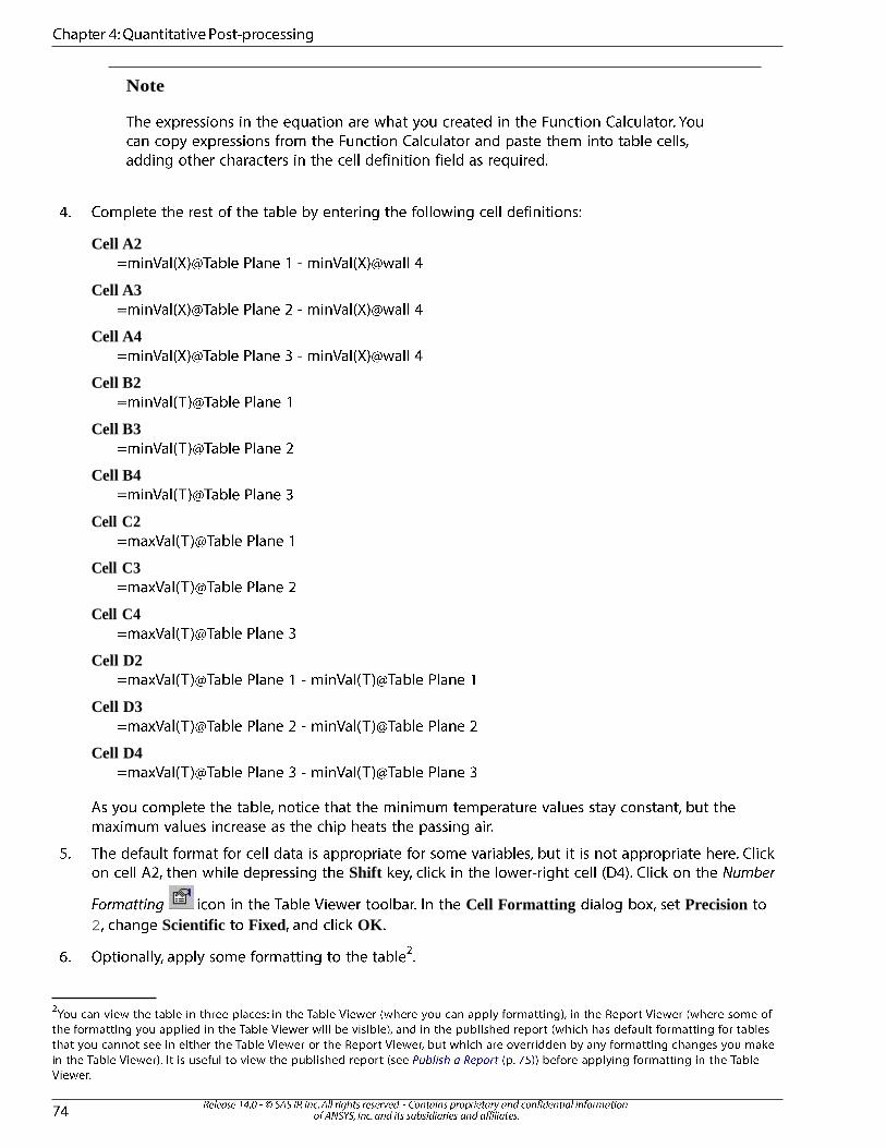
Note

Cell A2

Cell A3

Cell A4

Cell B2

Cell B3

Cell B4

Cell C2

Cell C3

Cell C4

Cell D2

Cell D3

Cell D4

Shift

Cell Formatting Precision

2 Scientific Fixed OK

4.11. Publish a Report

Report Viewer

Publish Report Viewer

Publish Report IC_Cooling_Sim-

ulation.htm

Tip

Publish Report

OK

Cfd Post Ansys

Documents

Transcript of Cfd Post Ansys