Citation: Ebrahimi, Mohammadreza and Crapper, Martin (2017) CFD-DEM Simulation of Turbulence Modulation in Horizontal Pneumatic Conveying. Particuology, 31. pp. 15-24. ISSN 1674-2001

Published by: Elsevier

URL: http://dx.doi.org/10.1016/j.partic.2016.05.012 <http://dx.doi.org/10.1016/j.partic.2016.05.012>

This version was downloaded from Northumbria Research Link: http://nrl.northumbria.ac.uk/26988/

Northumbria University has developed Northumbria Research Link (NRL) to enable users to access the University’s research output. Copyright ©  and moral rights for items on NRL are retained by the individual author(s) and/or other copyright owners. Single copies of full items can be reproduced, displayed or performed, and given to third parties in any format or medium for personal research or study, educational, or not-for-profit purposes without prior permission or charge, provided the authors, title and full bibliographic details are given, as well as a hyperlink and/or URL to the original metadata page. The content must not be changed in any way. Full items must not be sold commercially in any format or medium without formal permission of the copyright holder. The full policy is available online: http://nrl.northumbria.ac.uk/policies.html

This document may differ from the final, published version of the research and has been made available online in accordance with publisher policies. To read and/or cite from the published version of the research, please visit the publisher’s website (a subscription may be required.)

CFD-DEM Simulation of Turbulence Modulation in Horizontal Pneumatic

Conveying

Mohammadreza Ebrahimi1, Martin Crapper2

1Institute for Infrastructure and Environment, School of Engineering, the University of Edinburgh, Edinburgh

EH9 3JL, UK

2Department of Mechanical and Construction Engineering, Northumbria University, Ellison Place, Newcastle-

upon-Tyne, NE1 8ST, UK

Abstract

A study is presented to evaluate the capabilities of the standard k-turbulence model and the

k-turbulence model with added source terms in predicting the experimentally measured

turbulence modulation due to the presence of particles in horizontal pneumatic conveying, in

the context of a CFD-DEM Eulerian-Langrangian simulation. Experiments were performed

using a 6.5 m long, 0.075 m diameter horizontal pipe in conjunction with a laser Doppler

anemometry (LDA) system. Spherical glass beads with two different sizes, 1.5 mm and 2 mm,

were used. Simulations were carried out using the commercial Discrete Element Method

(DEM) software EDEM, coupled with the Computational Fluid Dynamics (CFD) package

FLUENT. Hybrid source terms were added to the conventional k- turbulence model to take

into account the influence of the dispersed phase on the carrier phase turbulence intensity. The

simulation results showed that the turbulence modulation depends strongly on the model

parameter Cɛ3. Both the standard k- turbulence model and the k- turbulence model with the

hybrid source terms could predict the gas phase turbulence intensity trend only generally, with

in all cases a noticeable discrepancy between simulation and experimental results was

observed, particularly for the regions close to the pipe wall. It was also observed that in some

cases the addition of the source terms to the k- turbulence model did not improve the

simulation results when compared to the simulation results of the standard k- turbulence

model, though in the lower part of the pipe where particle loading was greater due to

gravitational effects the model with added source terms performed somewhat better.

Keywords: Turbulence modulation, Pneumatic conveying, Eulerian-Lagrangian approach, Laser

Doppler anemometry

1. INTRODUCTION AND BACKGROUND

1.1. Turbulence Modulation in Fluid-Particle Flows

Carrier phase turbulence structure changes as a particulate phase is added to a clear fluid phase.

This phenomenon is referred to as turbulence modulation in the literature (Elgobashi & Abou-

Arab, 1983). It is important because any change in continuous phase turbulence has a direct

influence on the fluid mean velocity, heat and mass transfer as well as particle mixing and

dispersion (Fokeer, Kingman, Lowndes, & Reynolds, 2004; Kenning & Crowe, 1997;

Lightstone & Hodgson, 2004). It has also been pointed out that in a dilute phase particle laden

flow, turbulence modulation impacts drastically on the conveying line pressure drop (Curtis &

van Wachem, 2004). Laín, Bröder, Sommerfeld, and Göz (2002) also highlighted the influence

of turbulence modulation on the prediction of the hydrodynamic behaviour of a bubble in a

bubble column. Therefore it seems that understanding the interaction between a dispersed

phase and fluid phase turbulence is one of the crucial steps in understanding the complex

characteristics of two-phase systems.

Both attenuation and augmentation of fluid phase turbulence have been reported in previous

studies. Despite much research focused on this topic, there is no generally accepted explanation

for the influence of the solid phase on the carrier phase (Crowe, 2000; Mandø, 2009). In

general, it is recognizable from previous studies that small particles tend to suppress the carrier

phase turbulence level while large particles increase it. Previous observations reveal that small

particles (particle diameter dp < 200 m) follow the fluid flow and as a result these particles

may break turbulent eddies. These small particles may be accelerated by eddies, and so extract

kinetic energy from them (dissipation of energy), leading to a reduction in the turbulence level

of the fluid flow (Geiss, et al., 2004; Lightstone & Hodgson, 2004). On the other hand, fluid

flow turbulence augmentation by large particles can be explained as a result of the wake

generated behind the particles. This wake creates an additional disturbance to the flow which

may increase the level of turbulence. These phenomena are considered to be the core reasons

of turbulence reduction and enhancement (Bolio & Sinclair, 1995).

In addition to these two predominant mechanisms, other factors such as fluid flow turbulence

modification due to particle-particle interaction, changes in turbulence dissipation as a result

of the introduction of new length scales and changes in the continuous phase velocity gradient

are believed to be other influential reasons for turbulence modification. However, these

mechanisms may be negligible in a dilute particle suspension (Yuan & Michaelides, 1992).

Lightstone and Hodgson (2004) also mentioned the influence of the crossing trajectory, i.e. the

relative mean velocity between the particles and the turbulence eddies, as another source of gas

phase turbulence generation.

Some researchers have tried to formulate turbulence modulation based on the observation of

experimental results (Crowe, 2000; Mandø, 2009). However these formulations are valid only

for the specific range of solid loading ratios and system specifications observed in each case.

According to the explanation regarding the turbulence modulation, it seems that particle size,

particle concentration (loading), fluid velocity and ratio of particle to fluid length scale are

important parameters to evaluate the turbulence modulation. These four parameters may be

expressed as 1) mass /volumetric solid loading, 2) the ratio of particle diameter to the fluid

turbulence length scale 3) particle Reynolds number (𝑅𝑒𝑝 = 𝜌(𝑣 − 𝑢𝑝)𝑑𝑝 𝜇⁄ ) and 4) Stokes

number (𝑆𝑡 = 𝜏𝑝 𝜏𝑒⁄ ) (Fokeer, et al., 2004; Gouesbet & Berlemont, 1998; Mandø, 2009; Yarin

& Hetsroni, 1994) where 𝜌 is the fluid density, 𝑣 is the fluid velocity, 𝑢𝑝 is the particle velocity,

𝑑𝑝 is particle diameter and 𝜇 is the dynamic viscosity. 𝜏𝑝 and 𝜏𝑒 are particle response time and

eddy turnover time respectively.

Based on the Elghobashi (1994) study, for particle volume fraction less than 10-6, the influence

of particles on the fluid phase turbulence is weak. For particle volume fractions in the range

10-6 < ϕ𝑝<10-3, the particles can augment or attenuate the carrier phase turbulence depending

on the ratio of 𝜏𝑝 𝜏𝑒⁄ . For 𝜏𝑝 𝜏𝑒⁄ < 1, the turbulence is reduced by the particle presence while

for 𝜏𝑝 𝜏𝑒⁄ > 1 the carrier phase turbulence is enhanced. Elghobashi (1994) also explained

turbulence augmentation due to the wake formation.

Gore and Crowe (1989) reviewed the wide range of experimental data for pipe and jet flows

and suggested that the ratio of particle diameter (dp) to the integral length scale (le) may be used

as a criterion to examine the augmentation or attenuation of turbulence level. The length scale

ratio 0.1 is a distinguishing point for turbulence modulation; for a length scale ratio dp/le <0.1

turbulence intensity decreases while for dp/le >0.1, particles tend to increase the turbulence

intensity.

Hetsroni (1989) investigated various experimental data for horizontal and vertical two-phase

pipe flows and concluded that particles with Rep higher than 400 tend to increase the turbulence

intensity due to vortex shedding from particles, while particles with Rep less than 400 tend to

suppress the turbulence intensity. Yuan and Michaelides (1992) also noted that a wake behind

a particle is formed for Rep > 20 and for Rep > 400 vortices are shed behind the solid particles.

Lun (2000) also reported that turbulence modulation depends significantly on Rep; however he

found vortex shedding occurs when Rep is around 300. He observed that particles tend to

attenuate the carrier phase turbulence when Rep < 300, whilst on the other hand if the Rep is

more than a critical Rep, turbulence enhances.

1.2. Previous Experimental Work on Turbulence Modulation

As laser Doppler anemometry (LDA) is a non-contact optical measurement which can handle

velocity components with high temporal and spatial resolution, it has been used extensively for

measuring gas and particle velocities in gas-solid flows (Fan, Zhang, Cheng, & Cen, 1997; Y.

Lu, Glass, Easson, & Crapper, 2008; Y. Lu, Glass, & Easson, 2009; Mathisen, Halvorsen, &

Melaaen, 2008; Tsuji & Morikawa, 1982). Tsuji and Morikawa (1982) observed that air flow

turbulence level depended heavily on particle size, that 3.4 mm particles increased the

turbulence while 0.2 mm particles reduced it. The influence of the particle size on the carrier

phase turbulence level also reported by (Tsuji, Morikawa, & Shimoni, 1984) and (Henthorn,

Park, & Curtis, 2005). Fan, et al. (1997) applied laser Doppler anemometry (LDA) to measure

both phases’ velocity and turbulence intensity in dilute vertical pneumatic conveying and

compared experimental measurements with simulation. They concluded that the turbulence

intensity of the gas phase was attenuated and the mean gas velocity profile was flattened by

adding particles. Turbulence intensity reduction by adding fine particles (50-90 m) was also

mentioned by Kulick, Fessler, and Eaton (1994) observing that the degree of attenuation

increased by increasing the particle mass loading ratio and distance from the wall.

1.3. Numerical Modelling of Turbulence Modulation

Generally, to model the turbulence modulation phenomenon, source terms are added to the

single phase flow equations for turbulent kinetic energy and dissipation to take into account

the presence of the solid phase. Some research has been conducted to formulate these source

terms (Geiss, et al., 2004; Gouesbet & Berlemont, 1998; Rao, Curtis, Hancock, & Wassgren,

2012). These formulations mainly depend on the turbulence model used to close the fluid

momentum equation (Laín & Sommerfeld, 2003). Since the k is the most common

turbulence model in single phase flow modelling, consequently most of the source terms are

derived for turbulent kinetic energy and dissipation equations of this model (Chen & Wood,

1985; Fan, et al., 1997; Pakhomov, Protasov, Terekhov, & Varaksin, 2007). However, source

terms for other turbulence models like Reynolds stress turbulence model and k- have also

been derived (Laín & Sommerfeld, 2008; Lun, 2000). These source terms can be divided into

three main methods based on the original equations that these source terms have been derived

from (Boulet & Moissette, 2002; Laín, et al., 2002; Mandø, 2009). These are standard,

consistent and hybrid methods. In fact, the hybrid method is the combination of standard and

consistent methods (Mandø, 2009). Here, these categories are explained for k- turbulence

model.

1.3.1. Standard and Consistent Approaches

The general form of the source term due to the dispersed phase in the turbulent kinetic energy

equation for the standard method may be expressed as equation (1) (Chen & Wood, 1985;

Gouesbet & Berlemont, 1998):

𝑆𝑘𝑝 = 𝑆𝑝𝑣𝑖′ 𝑣𝑖

′ (1)

where 𝑆𝑘𝑝 is the source term in the turbulent kinetic energy equation and 𝑆𝑝𝑣𝑖

′ is the source term

in fluctuating momentum exchange term. If we assume that the interaction between the two

phases occurs only due to the drag force, then equation (1) can be written as

𝑆𝑘𝑝 =ϕ𝑝𝜌𝑝

𝜏𝑝(𝐶𝐷)(𝑢𝑝𝑖

′ 𝑣𝑖′ − 𝑣𝑖

′𝑣𝑖′) (2)

where ϕ𝑝, 𝜌𝑝 and 𝐶𝐷 represent the particle volume fraction, particle density and drag

coefficient respectively. 𝑣𝑖′ is gas fluctuating velocity and 𝑢𝑝𝑖

′ is particle fluctuating velocity.

𝑣𝑖′𝑣𝑖

′ is modelled as for the clear gas phase as used in the standard k model, which is 𝑣𝑖′𝑣𝑖

′ =

2𝑘. However 𝑢𝑝𝑖′ 𝑣𝑖

′ still requires to be modelled (Lightstone & Hodgson, 2004). Some models

have been presented in Lightstone and Hodgson (2004) for the k model. As stated by Boulet

and Moissette (2002), 𝑢𝑝𝑖′ arises from particle-particle and particle-wall interaction, and is often

smaller than 𝑣𝑖′ resulting in 𝑆𝑘𝑝 being negative. Therefore, this approach can only predict the

dissipation of the carrier phase turbulence (Boulet & Moissette, 2002; Laín, et al., 2002;

Mandø, 2009). One may conclude that this method is not suitable for the modelling of

turbulence modulation due to large particles which enhance turbulence intensity.

The consistent method derives from Crowe (2000). It starts with the mechanical energy

equation for the fluid phase. The source term in the turbulent kinetic energy equation

considering the drag force as the only interaction force is expressed as:

𝑆𝑘𝑝 =ϕ𝑝𝜌𝑝

𝜏𝑝(𝐶𝐷)(|𝑣𝑖 − 𝑢𝑝𝑖|

2+ (𝑢𝑝𝑖

′ 𝑢𝑝𝑖′ − 𝑣𝑖

′𝑢𝑝𝑖′ )) (3)

The first contribution may be explained as the kinetic energy production due to the particle

drag. In fact, this term takes into account turbulence generation due to the particle wake. The

second term (redistribution) is attributed to the transfer of the kinetic energy of the particle

motion into the kinetic energy of the continuous phase. This second term has a negligible effect

in dilute suspensions. Hwanc and Shen (1993) also presented the same formulation, however

they did not limit the momentum exchange term to the drag force.

Since larger and heavier particles are conveyed with lower velocity, the first term in equation

(3) has a higher value when compared to the conveying of smaller particles which are conveyed

with higher velocity. Generally, the generation due to the particle drag has a larger magnitude

than the redistribution term. As a result one may notice that models based on this approach are

capable of capturing fluid phase turbulence augmentation only, and may not be suitable to be

applied for turbulence modulation due to small particles.

1.3.2. Hybrid Method

With regard to the limitations of the previous methods of simulating turbulence modulation,

the hybrid method was suggested by (Geiss, et al., 2004). The hybrid source term for the

kmodel can be seen in equation (4). Only the drag force was considered as a gas-solid

interaction force and the influence of particle-particle collisions on the turbulence modulation

was neglected.

𝑆𝑘𝑝 =ϕ𝑝𝜌𝑝

𝜏𝑝(𝐶𝐷)(|𝑣𝑖 − 𝑢𝑝𝑖|

2+ (𝑢𝑝𝑖

′ 𝑢𝑝𝑖′ − 𝑣𝑖

′𝑣𝑖′)) (4)

This source term can also be derived by adding the standard and consistent method source

terms (Mandø, 2009). As mentioned for the consistent approach, the first term represents the

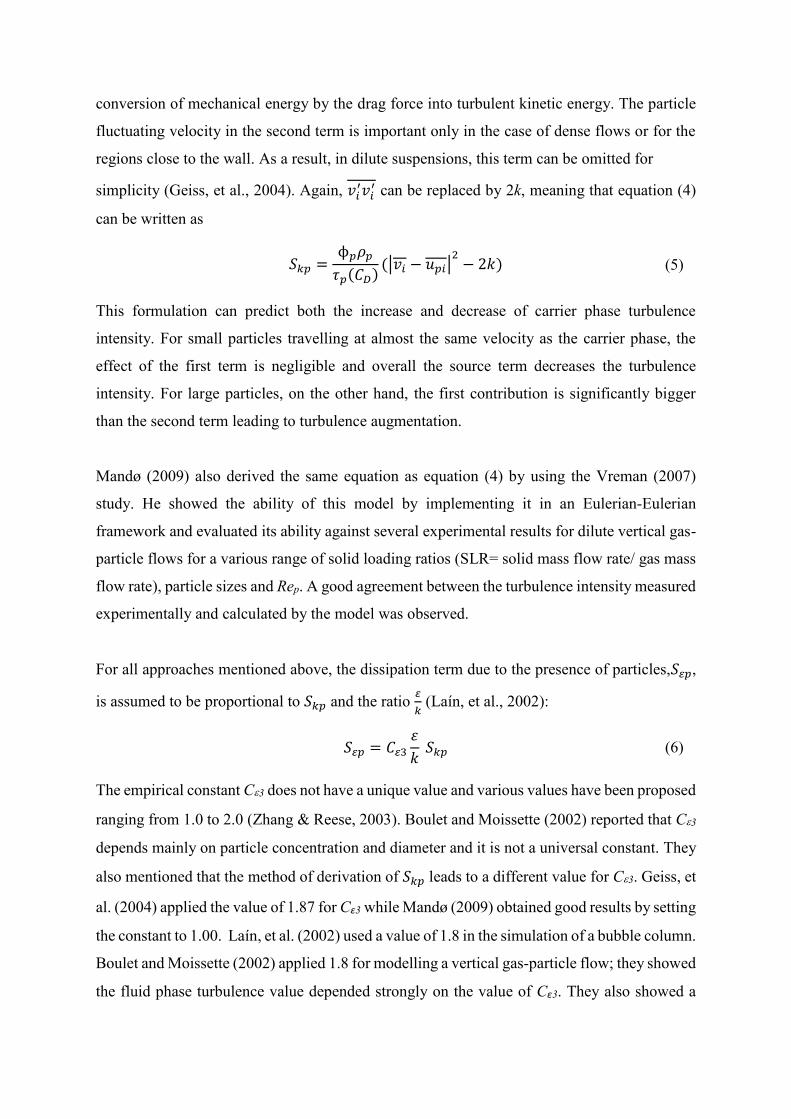
conversion of mechanical energy by the drag force into turbulent kinetic energy. The particle

fluctuating velocity in the second term is important only in the case of dense flows or for the

regions close to the wall. As a result, in dilute suspensions, this term can be omitted for

simplicity (Geiss, et al., 2004). Again, 𝑣𝑖′𝑣𝑖

′ can be replaced by 2k, meaning that equation (4)

can be written as

𝑆𝑘𝑝 =ϕ𝑝𝜌𝑝

𝜏𝑝(𝐶𝐷)(|𝑣𝑖 − 𝑢𝑝𝑖|

2− 2𝑘) (5)

This formulation can predict both the increase and decrease of carrier phase turbulence

intensity. For small particles travelling at almost the same velocity as the carrier phase, the

effect of the first term is negligible and overall the source term decreases the turbulence

intensity. For large particles, on the other hand, the first contribution is significantly bigger

than the second term leading to turbulence augmentation.

Mandø (2009) also derived the same equation as equation (4) by using the Vreman (2007)

study. He showed the ability of this model by implementing it in an Eulerian-Eulerian

framework and evaluated its ability against several experimental results for dilute vertical gas-

particle flows for a various range of solid loading ratios (SLR= solid mass flow rate/ gas mass

flow rate), particle sizes and Rep. A good agreement between the turbulence intensity measured

experimentally and calculated by the model was observed.

For all approaches mentioned above, the dissipation term due to the presence of particles,𝑆𝜀𝑝,

is assumed to be proportional to 𝑆𝑘𝑝 and the ratio 𝜀

𝑘 (Laín, et al., 2002):

𝑆𝜀𝑝 = 𝐶𝜀3

휀

𝑘 𝑆𝑘𝑝 (6)

The empirical constant C3 does not have a unique value and various values have been proposed

ranging from 1.0 to 2.0 (Zhang & Reese, 2003). Boulet and Moissette (2002) reported that C3

depends mainly on particle concentration and diameter and it is not a universal constant. They

also mentioned that the method of derivation of 𝑆𝑘𝑝 leads to a different value for C3. Geiss, et

al. (2004) applied the value of 1.87 for Cɛ3 while Mandø (2009) obtained good results by setting

the constant to 1.00. Laín, et al. (2002) used a value of 1.8 in the simulation of a bubble column.

Boulet and Moissette (2002) applied 1.8 for modelling a vertical gas-particle flow; they showed

the fluid phase turbulence value depended strongly on the value of Cɛ3. They also showed a

small change in the Cɛ3 value (from 1.8 to 1.85 or 1.8 to 1.81) could change the simulation

results considerably. They concluded that the value of Cɛ3 which gives the best result for one

example may not be suitable for another example if there is a change in the volume fraction.

Zhang and Reese (2003) reported that, for large and heavy particles with the ratio of the particle

relaxation time to time scale of the large eddies around 10, C3 was decreased by increasing the

mass loading. They proposed to replace the C3 in equation (6) with C3,c based on equation (7),

which is dependent on the particle volume fraction:

𝐶𝜀3,𝑐 = [1 − (6ϕ𝑝

𝜋ϕ𝑝,𝑚)

13⁄

] 𝐶𝜀3 (7)

where ϕ𝑝,𝑚 is the random close-packing particle volume fraction, which is assumed to be 0.64.

As can be seen from equation (7), Cɛ3,c depends on the initial selection of Cɛ3 .They selected

the value of 1.95 for Cɛ3 which best matches Tsuji and Morikawa (1982)’s experimental

results, and also showed that the predicted turbulent kinetic energy depended significantly on

the value of Cɛ3.

In summary the number of studies covering the simulation of turbulence modulation in particle

laden flow is very limited and our study is intended to begin addressing this situation.

1.4. Aims

The aim of our study is to evaluate the capabilities of the standard k-turbulence model and

the k-turbulence model with added source terms in predicting the experimentally measured

turbulence modulation in horizontal pneumatic conveying in the context of a CFD-DEM

Eulerian-Langrangian simulation. To achieve this goal, a series of experiments was conducted

to measure the turbulence level of the gas phase in the presence of particles using the LDA

technique in a horizontal pneumatic conveying line. The hybrid source terms were added to the

conventional k- turbulence model in the FLUENT-EDEM, CFD-DEM framework via User-

Defined Functions (UDF) and the simulation results were compared with the experimental data.

2. EXPERIMENTS

Figure 1 displays the schematic sketch of the horizontal pneumatic conveying experiment. The

y negative direction is in the gravity direction, the z positive axis is along the pipe and the x

positive direction is outward from the page. The pneumatic conveying system consists of a

hopper, fan, cyclone and conveying line. The particles are pushed by a screw feeder into the

inclined pipe (inclined at 45°) which is connected to the horizontal pipe. Once inside the

horizontal pipe, the fan sucks both the gas (air) and the particles into the cyclone at the

downstream end, where they are separated. The horizontal section is 6.5 m long and is

connected to the vertical section (1.2 m) by a bend. The pipe internal diameter is 0.075 m.

Measurements were carried out for a cross section at distance of 2 m from the point where the

particles are introduced to the horizontal section (shown by the red arrow). This cross section

is called z=2 m. The particle flow rate can be regulated by adjusting the screw feeder speed

and air flow rate can also be regulated; this makes it possible to obtain the desired SLRs in the

conveying line. Two different glass bead particles (spherical, diameters of 2 mm and 1.5 mm,

2540 kg/m3 density) were used in the experiments. Two different SLRs were produced by

combining the two different mean gas velocities (9.5 and 8.5 m/s) with fine adjustment of the

screw feeder speed. Particle flow rates were set to 0.1128 kg/s and 0.1329 kg/s. The resulting

SLRs were 2.3 and 3.

The LDA technique is used to measure the axial mean gas velocity and axial fluctuating root

mean square velocity (𝑣𝑟𝑚𝑠′ ) . The laser beams are refracted while passing through the pipe’s

curved wall. As a result, there would be a deviation between the actual beam intersection point

and the expected position, so in order to find the intersection point accurately inside the pipe

the method suggested by Y. Lu, et al. (2009) was adopted .

The first velocity measurement was at the pipe centre, and then the probes were moved

horizontally and vertically to measure the mean gas velocity and 𝑣𝑟𝑚𝑠′ for other measurement

points across the pipe. The distance between every two measurement points is 5 mm. In total,

twenty six velocity measurements were performed for the pipe cross section, including thirteen

measurements in the horizontal direction and thirteen measurements in the vertical direction.

The measurement reproducibility was checked by repeating the measurements three times, and

each measurement was carried out for 50 seconds. For the present study, the size difference

between the tracer particles (incense smoke) and the glass beads is considerable, ensuring that

only one velocity (carrier phase or solid phase) was measured at any given time.

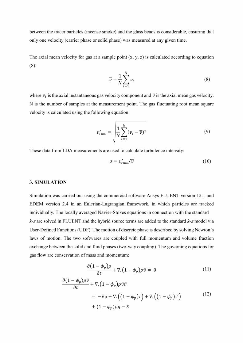
The axial mean velocity for gas at a sample point (x, y, z) is calculated according to equation

(8):

𝑣 =1

𝑁∑ 𝑣𝑖

𝑁

𝑖=1

(8)

where 𝑣𝑖 is the axial instantaneous gas velocity component and �̅� is the axial mean gas velocity.

N is the number of samples at the measurement point. The gas fluctuating root mean square

velocity is calculated using the following equation:

𝑣𝑟𝑚𝑠′ = √

1

𝑁∑(𝑣𝑖 − 𝑣)2

𝑁

𝑖=1

(9)

These data from LDA measurements are used to calculate turbulence intensity:

𝜎 = 𝑣𝑟𝑚𝑠′ 𝑣⁄ (10)

3. SIMULATION

Simulation was carried out using the commercial software Ansys FLUENT version 12.1 and

EDEM version 2.4 in an Eulerian-Lagrangian framework, in which particles are tracked

individually. The locally averaged Navier-Stokes equations in connection with the standard

k- are solved in FLUENT and the hybrid source terms are added to the standard k-model via

User-Defined Functions (UDF). The motion of discrete phase is described by solving Newton’s

laws of motion. The two softwares are coupled with full momentum and volume fraction

exchange between the solid and fluid phases (two-way coupling). The governing equations for

gas flow are conservation of mass and momentum:

𝜕(1 − 𝜙𝑝)𝜌

𝜕𝑡+ ∇. (1 − 𝜙𝑝)𝜌�̅� = 0 (11)

𝜕(1 − 𝜙𝑝)𝜌�̅�

𝜕𝑡+ ∇. (1 − 𝜙𝑝)𝜌�̅��̅�

= −∇p + ∇. ((1 − 𝜙𝑝)𝜏) + ∇. ((1 − 𝜙𝑝)𝜏′)

+ (1 − 𝜙𝑝)𝜌𝑔 − 𝑆

(12)

𝑆 =∑ 𝐹𝑖𝑛𝑡𝑒𝑟𝑎𝑐𝑡𝑖𝑜𝑛,𝑖

𝑛𝑖

Δ𝑉 (13)

𝜏 is the fluid viscous stress tensor, 𝜏′ is the Reynolds stress tensor, 𝑆 is the volumetric force

acting on each mesh cell and 𝐹𝑖𝑛𝑡𝑒𝑟𝑎𝑐𝑡𝑖𝑜𝑛,𝑖 includes drag and lift forces. 𝑛 and Δ𝑉 are the

number of particles in the considered computational cell and the computational cell volume

respectively. Drag force was simulated by the Ergun (1952) and Wen and Yu (1966) model.

In our previous study Ebrahimi, Crapper, and Ooi (2014) it was found that, the inclusion of

Magnus lift force due to particle rotation was essential to reproduce the general behaviour

observed in the experiments. Therefore, the Magnus lift force equation based on the Oesterlé

and Dinh (1998) research was implemented in the all simulations. The general k- turbulence

model equations in FLUENT are expressed as follow:

𝜕

𝜕𝑡(𝜌𝑘) +

𝜕

𝜕𝑥𝑖

(𝜌𝑘𝑣𝑖)

=𝜕

𝜕𝑥𝑖[(𝜇 +

𝜇𝑡

𝜎𝑘)

𝜕𝑘

𝜕𝑥𝑖] + 𝐺𝑘 + 𝐺𝑏 − 𝜌휀 − 𝑌𝑀

+ 𝑆𝑘𝑝

(14)

𝜕

𝜕𝑡(𝜌휀) +

𝜕

𝜕𝑥𝑖

(𝜌휀𝑣𝑖𝑣𝑖)

=𝜕

𝜕𝑥𝑖[(𝜇 +

𝜇𝑡

𝜎𝜀)

𝜕휀

𝜕𝑥𝑖] + 𝐶𝜀1

휀

𝑘(𝐺𝑘 + 𝐶𝜀3𝐺𝑏)

− 𝐶𝜀2𝜌휀2

𝑘+ 𝑆𝜀𝑝

(15)

𝜇𝑡 = 𝜌𝐶𝜇𝑘2

𝜀 is the turbulent eddy viscosity , 𝜎𝑘 and 𝜎𝜀 are turbulence Prandtl numbers and 𝑆𝑘𝑝

and 𝑆𝜀𝑝 are replaced by the model suggested by Geiss, et al. (2004) and Mandø (2009) (hybrid

source terms equations (5) and (6)). Translational and rotational motions of particles are

determined by the equations below.

𝑚𝑖

𝑑𝑢𝑝,𝑖

𝑑𝑡= 𝑚𝑖𝑔 + ∑ 𝐹𝑐𝑜𝑛𝑡𝑎𝑐𝑡 𝑖,𝑗

𝑛

𝑗=1

+ ∑ 𝐹𝑖𝑛𝑡𝑒𝑟𝑎𝑐𝑡𝑖𝑜𝑛,𝑖

𝑛

𝑖=1

(16)

𝐼𝑖

𝑑ω𝑝,𝑖

𝑑𝑡= ∑ 𝑇 𝑖,𝑗

𝑛

𝑗=1

(17)

where 𝑚𝑖 is the mass of particle i, 𝑢𝑝,𝑖 is the particle i velocity, 𝐹𝑐𝑜𝑛𝑡𝑎𝑐𝑡 𝑖,𝑗 is the contact force

of particle i and particle j or wall and 𝐹𝑖𝑛𝑡𝑒𝑟𝑎𝑐𝑡𝑖𝑜𝑛,𝑖 shows the particle-fluid interaction. ω𝑝,𝑖 and

𝐼𝑖 are the angular velocity and moment of inertia of particle i, respectively and 𝑇 𝑖,𝑗 is the

torque of particle i that interacts with particle j or wall. A non-linear Hertz-Mindlin contact

model was applied in the simulation. Normal force and normal damping force are given by:

𝐹𝑛 =4

3𝑌∗𝛿𝑛

3 2⁄√𝑅∗ (18)

𝐹𝑛𝑑 = −2√5 6⁄ 𝛽√𝑆𝑛𝑚∗𝑉𝑛

𝑟𝑒𝑙 (19)

𝑆𝑛 = 2𝑌∗√𝑅∗𝛿𝑛 (20)

𝛽 =ln 𝑒

√ln 2𝑒 + 𝜋2 (21)

where 𝑌∗, 𝛿𝑛 , 𝑚∗, 𝑅∗, 𝑒 are the equivalent Young’s modulus, the normal overlap, the

equivalent mass, the equivalent radius and coefficient of restitution respectively. Tangential

force and damping are calculated by the following equations (Mindlin & Deresiewicz, 1953)

𝐹𝑡 = −𝑆𝑡𝛿𝑡 (22)

𝑆𝑡 = 8𝐺∗√𝑅∗𝛿𝑛 (23)

𝐹𝑡𝑑 = −2√5 6⁄ 𝛽√𝑆𝑡𝑚∗𝑉𝑡

𝑟𝑒𝑙 (24)

where 𝛿𝑡 is the tangential overlap and 𝐺∗is the equivalent shear modulus. The tangential force

is limited by the Coulomb friction (𝜇𝑠𝐹𝑛) where 𝜇𝑠 represents the static friction coefficient. If

the net tangential force reaches the frictional force then sliding occurs. The rolling friction is

accounted for by applying a torque to the contacting surfaces which is a function of normal

force 𝐹𝑛 and coefficient of rolling friction 𝜇𝑟.

𝜏𝑟,𝑖 = −𝜇𝑟𝐹𝑛𝑅𝑖𝜔𝑖 (25)

A three-dimensional mesh was built to simulate the experimental apparatus. Due to the

requirements of the CFD-DEM coupling, a fluid mesh size which was three to five times bigger

than the particle size was selected. However, it is one of the limitations in the coupled CFD-

DEM that the mesh size cannot be resolved finely and as a result the fluid detail may not be

captured accurately. The domain was divided into 205,490 tetrahedral mesh elements, with

397,376 nodes. To decrease the computational time, only 2.2 m of horizontal pipe was

simulated. The gas velocity profile at 2.2 m along the pipe was measured by the aid of LDA

and this experimentally measured velocity profile then was used as a boundary condition in the

simulation. Particles in the simulations are created in the inclined pipe attached to the horizontal

pipe, with an initial velocity of 0.0635 m/s in the x direction. This initial velocity is given to

the particles to replicate the screw feeder effect, since the screw feeder is not modelled

explicitly. The particles roll down the inclined pipe surface and are pulled down by the effect

of gravity into the horizontal pipe where they experience a gas flow similar to the experiments.

All parameters used in the pneumatic conveying simulation in FLUENT-EDEM are

summarized in Table 1.

4. RESULTS AND DISCUSSION

4.1. Simulation of Turbulence Intensity in Single Phase Flow

Firstly, the simulation results for single-phase turbulence intensity are compared with the

experimental measurements. As seen in Figure 2 and Figure 3, the simulations give good

agreement with the single phase experimental measurements.

4.2. Effect of the Constant Cɛ3 on Turbulence Modulation in Particle Laden Flow

To determine whether or not the Cɛ3 value had a significant effect on the simulation results,

four different values for Cɛ3, all reported in the literature, were selected. Simulation results for

horizontal profile of turbulence intensity at z=2 m for SLR=2.3 and SLR=3 in the presence of

2 mm glass beads are shown in Figure 4 and Figure 5. It is seen that the turbulence intensity

values depend strongly on the Cɛ3. For both cases, by increasing the Cɛ3 values from 1.1 to

1.89, turbulence intensity drops noticeably. This is in a good agreement with the Zhang and

Reese (2003) study which reported that the Cɛ3 values had a significant effect on fluctuating

gas velocity. It is also seen that for regions close to the wall, turbulence intensity increases

significantly.

Figure 6 shows the vertical profile of turbulence intensity of air in the presence of 2 mm glass

beads at z=2 m for SLR=2.3. These results also indicate that the turbulence intensity values

change considerably by changing Cɛ3. It is also seen that the higher the Cɛ3 value, the lower the

turbulence intensity. Moreover, it is seen that the turbulence intensity value is not symmetric;

it is higher in the lower section of the pipe because the number of particles here is higher and

lower in the pipe upper section where the particle concentration is much lower. This trend was

previously observed experimentally by (Tsuji & Morikawa, 1982).

If the simulation results presented in Figure 4 and Figure 5 are summarized in one graph, the

influence of SLR on the turbulence intensity for a constant Cɛ3 can be seen (Figure 7). For

instance, if turbulence intensity for SLR=2.3, Cɛ3=1.7 is compared with SLR=3, Cɛ3=1.7, it

becomes clear that the simulated turbulent intensity increases with increasing SLR. The same

trend is seen when SLR=2.3, Cɛ3=1.8 is compared with SLR=3, Cɛ3=1.8. It shows that the

turbulence intensity increases by increasing the SLR for a constant Cɛ3 as was previously

reported in Curtis & van Wachem, 2004.

The results from Figure 4 to Figure 7 confirm that the new source terms added to the k-

turbulence model are capable of predicting previously reported trends.

4.3. Comparison with Experimental Results

In order to evaluate the influence of the source terms added to the standard k-turbulence

model, simulation results were compared with experimental results. The results for horizontal

and vertical profiles of carrier phase turbulence intensity in the presence of 1.5 mm glass beads

with SLR=3 are shown in Figure 8 and Figure 9 respectively. It is seen that turbulence intensity

decreases with increasing the C3. In the horizontal profile, the k- model with the source terms

and C3=1.8 is under-predicting the experimental results considerably due to the overestimation

of the dissipation. Obviously, the turbulence intensity predicted by the k- turbulence model

with the source terms with C3=1.1 is over-predicting the turbulence intensity compared to the

experimental results in the central section of the pipe.

In the central regions of the pipe, the standard k- turbulence model without the source terms

can predict the experimental results more accurately when compared to the simulation results

with the k- turbulence model with the source terms. However, in the regions closer to the pipe

walls, the simulation results with the k- turbulence model with the source terms and C3=1.5

or 1.7 are closer to the experimental data when compared with the simulation results obtained

by the standard k- turbulence model. The experimental turbulence intensity trend is captured

only very generally by the turbulence models in the horizontal profile, and the model shows

significant turbulence intensity increase only for regions very close to the pipe wall.

As is seen, the experimentally measured turbulence intensity data is non-symmetric along the

horizontal profile. This can be explained by the fact that the particles enter at one side of the

inclined pipe, which is then connected to the horizontal pipe (please refer to Figure 1), so it can

be expected that there is a different particle number in x direction, and as a result non-

symmetric experimental data was measured.

In the vertical profile, the simulation results obtained from the standard k- turbulence model

are closer to the experimental data in the central region of pipe compared to the simulation

results obtained from the k- turbulence model with source terms. However, since there is no

term in the standard k- turbulence model to take into account the presence of particles, the

increase in turbulence intensity in the lower region of pipe where more particles are

concentrated due to gravity cannot be modelled accurately. Similar to the experimental

measurements, the k-turbulence model with the source terms and C3=1.1, 1.5 or 1.7 predicts

higher turbulence intensity values in the lower half of the pipe which are relatively close to the

experimental data. Lower turbulence intensity values in the pipe upper section where fewer

particles are transported are obtained when compared to the turbulence intensity values in the

pipe lower section by turbulence model with or without source terms. For both horizontal and

vertical profiles, the discrepancy between experimental and simulation results increases toward

the walls as previously observed by Boulet and Moissette (2002) in vertical pneumatic

transportation.

The capacity of the CFD-DEM approach to simulate the near-wall flow is generally limited, as

the fluid mesh cannot be resolved finely enough for this due to the requirement for it to be

significantly larger than the particle diameter. Moreover, in the implemented hybrid source

terms, the effect of the particle fluctuating velocity i.e. 𝑢𝑝𝑖′ 𝑢𝑝𝑖

′ was omitted for model

simplicity. However, for near-wall regions it can be imagined that the gas phase turbulence

intensity will be altered due to the significant increase of particle fluctuating velocity due to

the increased particle-wall collisions.

Simulation and experimental results of carrier phase turbulence intensity in the presence of 1.5

mm glass beads, SLR=2.3 are shown in Figure 10 and Figure 11. In the horizontal profile and

close to the pipe centre, a close agreement between the experimental data and the simulation

results obtained by the standard k- turbulence model is observed. The k- turbulence model

with the source terms over-estimates the turbulence intensity except for C3=1.8. Similar to

Figure 8, the model is not capable of capturing the detail of the experimental results. In the

vertical profile, the significant increase in the turbulent intensity in the lower section of pipe is

not captured by the standard k- turbulence model. In this case, the simulations with Cɛ3=1.7

or Cɛ3=1.1 are closest to the experimental results. The turbulence intensity trend is captured

generally by the k- turbulence model with the source terms.

Comparison between experimental and simulation results of horizontal and vertical profiles of

gas phase turbulence intensity in the presence of 2 mm glass beads for SLR=2.3 are presented

in Figure 12 and Figure 13. As can be seen, the simulation results with Cɛ3=1.8 or C3=1.7 are

close to the experimental results in the central section of the pipe in both horizontal and vertical

profiles. However, the discrepancy increases for the measurement points closer to the pipe

walls. Similar to the previous simulations, the turbulence intensity increases in the lower half

of the pipe is not captured by the standard k- turbulence model (Figure 13).

Figure 14 and Figure 15 show the carrier phase turbulence intensity for the particle laden flow

with 2 mm glass beads, SLR=3. As is seen, the simulation results obtained from the standard

k- turbulence model and the k- turbulence model with Cɛ3=1.8 are similar. A very good

agreement between the simulation with Cɛ3=1.8, the standard k- turbulence model and

experimental results in the horizontal profile is observed, except for the measurement points

close to the pipe walls. In the vertical profile, a good agreement is also observed between the

experimental results and simulation results with Cɛ3=1.8 in the central parts of the pipe (Figure

15).

From all comparisons between experimental and simulations results presented in this section,

it was observed that neither the k-turbulence model with hybrid source terms nor the standard

k-turbulence model could predict accurately the carrier phase turbulence intensity in a

horizontal pneumatic conveying experiment using a CFD-DEM approach. However, the

general behaviour was captured. It was found that in some cases the addition of source terms

could not improve the simulation results.

It also was observed that the turbulence model is very sensitive to the Cɛ3 values. Therefore, if

source terms are used, this value needs to be calibrated before every simulation depending on

the particle size and SLR. In the current study it was observed that as Cɛ3 reached 1.7 or 1.8 a

further increase of Cɛ3 values changed the simulation results significantly. However, more

simulations with various operating conditions (i.e. different SLRs) are required to be performed

before any conclusion can be made regarding the critical Cɛ3 values.

5. CONCLUSIONS

The turbulence modulation phenomenon was investigated experimentally and numerically. The

LDA technique was used to measure turbulence intensity in a horizontal pneumatic conveying

line in the presence of 1.5 and 2 mm spherical glass beads for two SLRs, 2.3 and 3. Simulations

were carried out in an Eulerian-Lagrangian framework using the commercially CFD-DEM

coupled code FLUENT-EDEM. User-defined functions were used to add hybrid source terms

to the standard k-turbulence model to simulate turbulence modulation due to particles.

Simulation results revealed that the simulated turbulence intensity depends on the value of the

constant Cɛ3 and the higher the Cɛ3, the lower the turbulence intensity. It was also shown that

the higher the SLR, the higher the turbulence intensity. In vertical profiles, simulation results

predicted the higher turbulence intensity at the lower section of the pipe, where the solid

volume fraction is higher due to gravity. This is in good agreement with the experimental

measurements.

Comparison between the experimental and simulation results showed that for all simulations,

the standard k-turbulence model and the k-turbulence model with hybrid source terms are

not capable of predicting the detail of turbulence intensity in horizontal and vertical profiles,

especially for the regions close to the pipe wall. However, the general trend of turbulence

intensity is captured. The standard k-turbulence model could not predict the turbulence

intensity increase in the lower section of the pipe where more particles are conveyed because

there is no term in the standard k-turbulence model to take into account the presence of

particles. It was also observed that in some cases the addition of source terms did not generally

improve the simulation results. Therefore, before initiating any simulations it may be needed

to check if these source terms are required based on the operating conditions. If these source

terms are applied, the Cɛ3 value needs to be calibrated. The results suggest that the k-

turbulence model is not well suited to modelling a particle-fluid system where turbulence

modulation is important, and there is thus a necessity to develop a turbulence model which can

be applied for such particle laden flows. Turbulence modulation source terms including the

particle-particle interaction and lift force effects may also be derived and implemented into a

CFD-DEM framework as a future study.

Acknowledgment

The authors wish to thank DEM-Solutions Limited for their assistance with this work.

This work has been carried out as a part of the PARDEM project, an EU-funded, Framework

7 Marie Curie Initial Training Network. The financial support provided by the European

Commission is gratefully acknowledged.

Nomenclature

𝐶𝐷 Drag coefficient Greek letters

𝑒 Coefficient of restitution 𝛿𝑛 Normal overlap(m)

𝐺∗ Equivalent shear modulus(pa) 𝛿𝑡 Tangential overlap(m)

𝐼𝑖 Particle moment of inertia(kg.m2) 휀 Dissipation (m2/s3)

𝑘 Turbulent kinetic energy(m2/s2) 𝜇 Dynamic viscosity(Pa.s)

𝑚𝑖 Particle mass(kg) 𝜇𝑟 Coefficient of rolling friction

𝑚∗ Equivalent mass(kg) 𝜇𝑠 Coefficient of static friction

𝑅∗ Equivalent radius(m) 𝜌 Fluid density(kg/m3)

𝑇𝑖,𝑗 Torque(N.m) 𝜌𝑝 Particle density(kg/m3)

𝑢𝑝 Particle velocity(m/s) 𝜏𝑒 Eddy turnover time(s)

𝑢𝑝𝑖′ Particle fluctuating velocity(m/s) 𝜏𝑟 Rolling friction

�̅�𝑝 Mean particle velocity(m/s) 𝜏𝑝 Particle response time(s)

𝑣𝑖′ Gas fluctuating velocity(m/s) ϕ𝑝

Particle volume fraction

�̅� Mean gas velocity (m/s)

𝑉𝑡𝑟𝑒𝑙 Relative tangential velocity(m/s)

𝑉𝑛𝑟𝑒𝑙 Relative normal velocity(m/s)

𝜔𝑝 Particle angular velocity(rad/s)

𝑌∗ Equivalent Young’s modulus(pa)

References:

Bolio, E. J., & Sinclair, J. L. (1995). Gas turbulence modulation in the pneumatic conveying

of massive particles in vertical tubes. International Journal of Multiphase Flow, 21,

985-1001.

Boulet, P., & Moissette, S. (2002). Influence of the particle-turbulence modulation modelling

in the simulation of a non-isothermal gas-slid flow. International Journal of Heat and

Mass Transfer, 45, 4201-4216.

Chen, C. P., & Wood, P. E. (1985). A turbulence closure model for dilute gas-particle flows.

The Canadian Journal of Chemical Engineering, 63, 349-360.

Crowe, C. T. (2000). On models for turbulence modulation in fluid-particle flows.

International Journal of Multiphase Flow, 26, 719-727.

Curtis, J. S., & van Wachem, B. (2004). Modeling particle-laden flows: A research outlook.

AIChE Journal, 50, 2638-2645.

Ebrahimi, M., Crapper, M., & Ooi, J. Y. (2014). Experimental and Simulation Studies of

Dilute Horizontal Pneumatic Conveying. Particulate Science and Technology, 32,

206-213.

Elghobashi, S. (1994). On predicting particle-laden turbulent flows. Applied Scientific

Research, 52, 309-329.

Elgobashi, S. E., & Abou-Arab, T. W. (1983). A two-equation turbulence model for two-

phase flows. Physics of Fluids, 26, 931-938.

Ergun, S. (1952). Fluid flow through packed columns. Chemical Engineering Progress, 48,

89-94.

Fan, J., Zhang, X., Cheng, L., & Cen, K. (1997). Numerical simulation and experimental

study of two-phase flow in a vertical pipe. Aerosol science and technology, 3, 281-

292

Fokeer, S., Kingman, S., Lowndes, I., & Reynolds, A. (2004). Characterisation of the cross

sectional particle concentration distribution in horizontal dilute flow conveying-a

review. Chemical Engineering and Processing: Process Intensification, 43, 677-691.

Geiss, S., Dreizler, A., Stojanovic, Z., Chrigui, M., Sadiki, A., & Janicka, J. (2004).

Investigation of turbulence modification in a non-reactive two-phase flow.

Experiments in Fluids, 36, 344-354.

Gore, R. A., & Crowe, C. T. (1989). Effect of particle size on modulating turbulent intensity.

International Journal of Multiphase Flow, 15, 279-285.

Gouesbet, G., & Berlemont, A. (1998). Eulerian and Lagrangian approaches for predicting

the behaviour of discrete particles in turbulent flows. Progress in Energy and

Combustion Science, 25, 133-159.

Henthorn, K. H., Park, K., & Curtis, J. S. (2005). Measurement and prediction of pressure

drop in pneumatic conveying: Effect of particle characteristics, mass loading, and

Reynolds number. Industrial & Engineering Chemistry Research, 44, 5090-5098.

Hetsroni, G. (1989). Particles-turbulence interaction. International Journal of Multiphase

Flow, 15, 735-746.

Hwanc, G. J., & Shen, H. H. (1993). Fluctuation energy equations for turbulent fluid-solid

flows. International Journal of Multiphase Flow, 19, 887-895.

Kenning, V. M., & Crowe, C. T. (1997). On the effect of particles on carrier phase turbulence

in gas-particle flows. International Journal of Multiphase Flow, 23, 403-408.

Kulick, J., Fessler, J., & Eaton, J. (1994). Particle response and turbulent modification in

fully-developed channel flow. JOURNAL OF FLUID MECHANICS, 277, 109-134.

Laín, S., Bröder, D., Sommerfeld, M., & Göz, M. (2002). Modelling hydrodynamics and

turbulence in a bubble column using the Euler–Lagrange procedure. International

Journal of Multiphase Flow, 28, 1381-1407.

Laín, S., & Sommerfeld, M. (2003). Turbulence modulation in dispersed two-phase flow

laden with solids from a Lagrangian perspective. International Journal of Heat and

Fluid Flow, 24, 616-625.

Laín, S., & Sommerfeld, M. (2008). Euler/Lagrange computations of pneumatic conveying in

a horizontal chanel with different wall roughness. Powder Technology, 184, 76-88.

Lightstone, M. F., & Hodgson, S. M. (2004). Turbulence Modulation in Gas-Particle Flows:

A Comparison of Selected Models. The Canadian Journal of Chemical Engineering,

82, 209-219.

Lu, Y., Glass, D., Easson, W. J., & Crapper, M. (2008). Investigation of Flow Patterns of

Gas-Solid Granular Flow over Horizontal Pipe Cross-sections by FLUENT & EDEM.

In Particulate Systems Analysis Stratford-upon-Avon, United Kingdom.

Lu, Y., Glass, D. H., & Easson, W. J. (2009). An investigation of particle behaviour in gas–

solid horizontal pipe flow by an extended LDA technique. Fuel, 88.

Lun, C. K. K. (2000). Numerical simulation of dilute turbulent gas-solid flows. International

Journal of Multiphase Flow, 26, 1707-1736.

Mandø, M. (2009). Turbulence modulation by non-spherical particles. Department of energy

technology, Aalborg University.

Mathisen, A., Halvorsen, B., & Melaaen, M. C. (2008). Experimental studies of dilute

vertical pneumatic transport. Particulate science and technology 26, 235-246.

Mindlin, R. D., & Deresiewicz, H. (1953). Elastic spheres in contact under varying oblique

forces. Journal of applied mechanics, 21, 327-344.

Oesterlé, B., & Dinh, T. B. (1998). Experiments on the lift of a spinning sphere in a range of

intermediate Reynolds numbers. Experiments in Fluids, 25, 16-22.

Pakhomov, M. A., Protasov, M. V., Terekhov, V. I., & Varaksin, A. Y. (2007). Experimental

and numerical investigation of downward gas-dispersed turbulent pipe flow.

International Journal of Heat and Mass Transfer, 50, 2107-2116.

Rao, A., Curtis, J. S., Hancock, B. C., & Wassgren, C. (2012). Numerical simulation of dilute

turbulent gas-particle flow with turbulence modulation. AIChE Journal, 58, 1381-

1396.

Tsuji, Y., & Morikawa, Y. (1982). LDV measurements of an air-solid two-phase flow in a

horizontal pipe. Journal of Fluid Mechanics, 120, 385-409.

Tsuji, Y., Morikawa, Y., & Shimoni, H. (1984). LDV measurements of an air-solid two-

phase flow in a vertical pipe. JOURNAL OF FLUID MECHANICS, 139, 417-434.

Vreman, A. W. (2007). Turbulence characteristics of particle-laden pipe flow. JOURNAL OF

FLUID MECHANICS, 584, 235-279.

Wen, C. Y., & Yu, Y. H. (1966). Mechanics of fluidisation. Chemical Engineering Progress

Symposium Series, 62, 100-111.

Yarin, L. P., & Hetsroni, G. (1994). Turbulence intensity in dilute two-phase flows- 3 The

particles-turbulence interaction in dilute two-phase flow. International Journal of

Multiphase Flow, 20, 27-44.

Yuan, Z., & Michaelides, E. E. (1992). Turbulence modulation in particulate flows- A

theoritical approach. Int J. Multiphase Flow, 18, 779-785.

Zhang, Y., & Reese, J. M. (2003). Gas turbulence modulation in a two-fluid model for gas–

solid flows. AIChE journal, 49, 3048-3065.

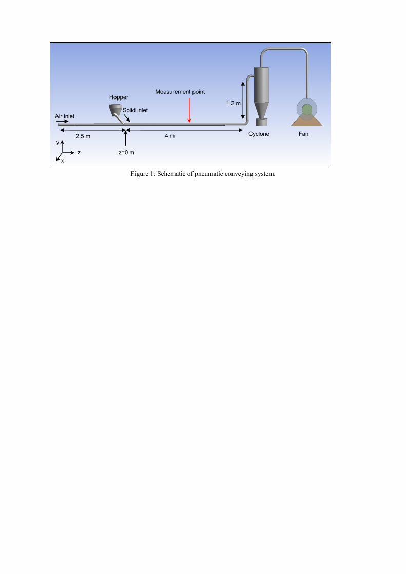
Figure 1: Schematic of pneumatic conveying system.

Cyclone Fan

1.2 m

4 m

Measurement point Hopper

2.5 m

Air inlet Solid inlet

z z=0 m

x

y

Figure 2: Horizontal profile of gas turbulence intensity for pure gas flow, gas velocity 9.5m/s.

Figure 3: Vertical profile of gas turbulence intensity for pure gas flow, gas velocity 8.5m/s.

Figure 4: Effect of C3 on the horizontal profile of turbulence intensity, 2 mm particles, SLR=2.3 at z=2 m.

Figure 5: Effect of C3 on the horizontal profile of turbulence intensity, 2 mm particles, SLR=3 at z=2 m

Figure 6: Effect of C3 on the vertical profile of turbulence intensity, 2 mm particles, SLR=2.3 at z=2 m.

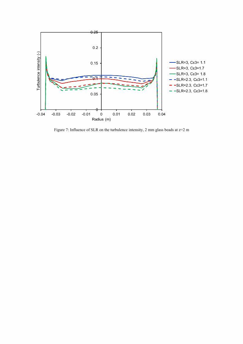
Figure 7: Influence of SLR on the turbulence intensity, 2 mm glass beads at z=2 m

Figure 8: Effect of C3 on the horizontal profile of turbulence intensity and comparison between simulation and

experimental results, 1.5 mm particles, SLR= 3 at z=2 m

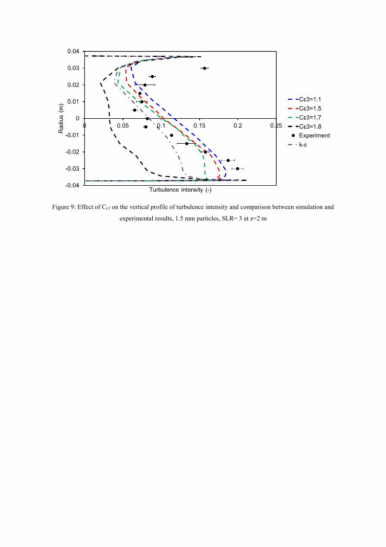
Figure 9: Effect of C3 on the vertical profile of turbulence intensity and comparison between simulation and

experimental results, 1.5 mm particles, SLR= 3 at z=2 m

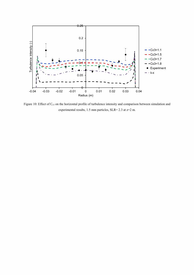
Figure 10: Effect of C3 on the horizontal profile of turbulence intensity and comparison between simulation and

experimental results, 1.5 mm particles, SLR= 2.3 at z=2 m.

Figure 11: Effect of C3 on the vertical profile of turbulence intensity and comparison between simulation and

experimental results, 1.5 mm particles, SLR= 2.3, at z=2 m

Figure 12: Effect of C3 on the horizontal profile of turbulence intensity and comparison between simulation

and experimental results, 2 mm particles, SLR= 2.3, at z=2 m.

Figure 13: Effect of C3 on the vertical profile of turbulence intensity and comparison between simulation and

experimental results, 2 mm particles, SLR= 2.3, at z=2 m.

Figure 14: Effect of C3 on the horizontal profile of turbulence intensity and comparison between simulation and

experimental results, 2 mm particles, SLR= 3 at z=2 m.

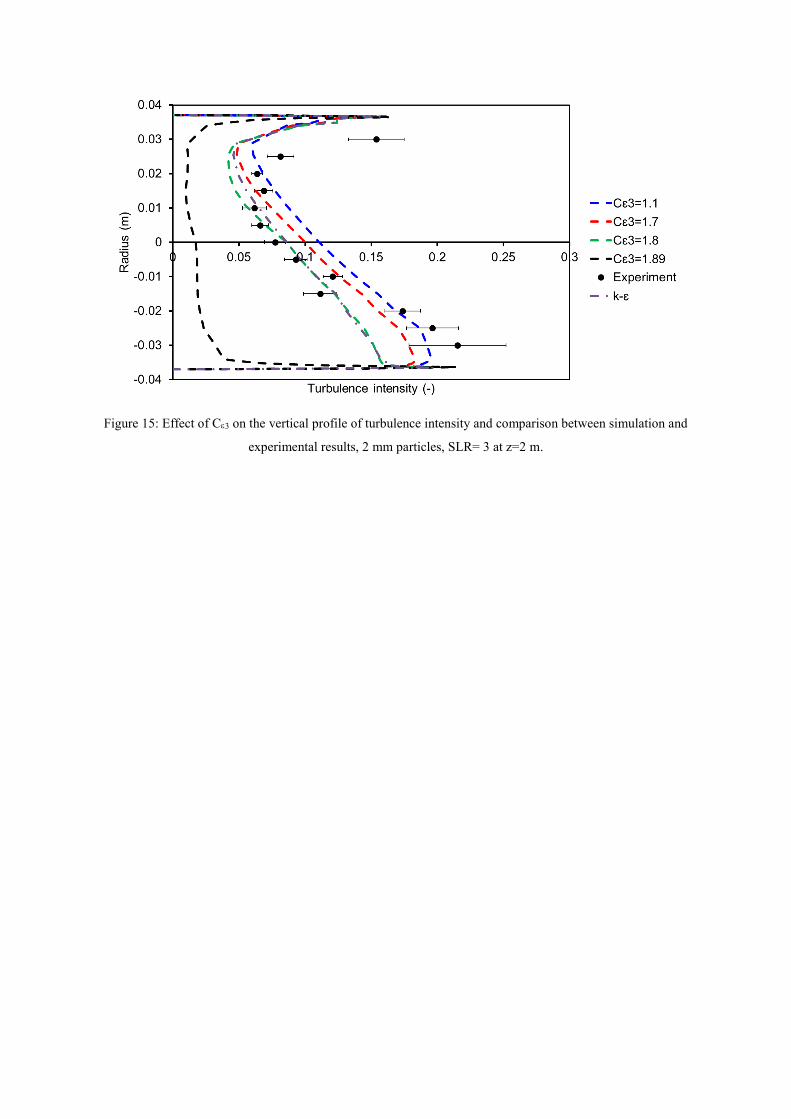
Figure 15: Effect of C3 on the vertical profile of turbulence intensity and comparison between simulation and

experimental results, 2 mm particles, SLR= 3 at z=2 m.

Table 1: Numerical parameters for FLUENT-EDEM simulation

Simulation method CFD-DEM (Eulerian-Lagrangian)

Coupling method Two-way coupling

FLUENT

Air density (kg/m3) 1.225

Air viscosity (pa.s) 1.78e-5

Wall boundary No-slip condition

Turbulence model Standard k- model or k- model with the

hybrid source terms

EDEM

Particle creation Created in the inclined pipe with the

initial velocity similar to the experiments

Particle flow rate (kg/s) 0.1128, 0.1329

Poisson’s ratio 0.24

Shear modulus(pa) 2.62e10

Particle-Particle, Particle-wall contact

model

Non-linear Hertz-Mindlin

Particle diameter (m) 0.0015, 0.002

Particle density (kg/m3) 2540

Coefficient of restitution (glass beads-

wall)

0.97

Coefficient of restitution (glass beads-

glass beads)

0.9

Coefficient of static friction 0.154

Coefficient of rolling friction 0.1

Time step 3.0e-7

Gas-Particle interactions

Drag model Ergun and Wen&Yu

Lift model Magnus lift force