Cetacean habitats in the northern Gulf of Mexico et al.: Cetacean habitats in the northern Gulf of...

219

Studies of cetacean distribution in the northern Gulf of Mexico have largely relied on stranding, opportunistic sight-ing, and limited survey data (Jefferson and Schiro, 1997) until recently (Mullin et al., 1994; Davis and Fargion1; Davis et al.2). During the past decade, both aerial and shipboard assessment sur-veys in the oceanic (>200 m depth) northern Gulf have identifi ed and char-acterized the abundance and distribu-tion of 20 species of cetaceans, all but one of which were odontocetes (Mullin et al., 1994; Mullin and Hansen, 1999; Hansen et al.3; Mullin and Hoggard4). Only two of these species, the bottle-

Cetacean habitats in the northern Gulf of Mexico

Mark F. BaumgartnerSoutheast Fisheries Science CenterNational Marine Fisheries ServiceBldg. 1103, Room 218John C. Stennis Space Center, Mississippi 39529Present address: College of Oceanic and Atmospheric Sciences Oregon State University 104 Ocean Administration Building Corvallis, Oregon 97331E-mail address: [email protected]

Keith D. MullinSoutheast Fisheries Science CenterNational Marine Fisheries ServiceP.O. Drawer 1207Pascagoula, Mississippi 39568

L. Nelson MayThomas D. LemingSoutheast Fisheries Science CenterNational Marine Fisheries ServiceBldg. 1103, Room 218John C. Stennis Space Center, Mississippi 39529

Manuscript accepted 11 October 2000.Fish. Bull. 99:219–239 (2001).

Abstract–Surveys were conducted in the northern Gulf of Mexico during the spring seasons of 1992, 1993, and 1994 to determine the distribution, abun-dance, and habitat preferences of oce-anic cetaceans. The distributions of bottle nose dolphins (Tursiops trunca-tus), Risso’s dolphins (Grampus griseus), Kogia spp. (pygmy [Kogia breviceps] and dwarf sperm whales [Kogia sima]), pantropical spotted dolphins (Stenella attenuata), and sperm whales (Physe-ter macrocephalus) were examined with respect to depth, depth gradient, surface temperature, surface temperature vari-ability, the depth of the 15°C isotherm, surface chlorophyll concentration, and epipelagic zooplankton biomass. Bottle-nose dolphins were encountered in two distinct regions: the shallow continen-tal shelf (0–150 m) and just seaward of the shelf break (200–750 m). Within both of these depth strata, bottlenose dolphins were sighted more frequently than expected in regions of high sur-face temperature variability which sug-gests an association with ocean fronts. Risso’s dolphins were encountered over the steeper sections of the upper con-tinental slope (200–1000 m), whereas the Kogia spp. were sighted more fre-quently in waters of the upper conti-nental slope that had high zooplankton biomass. The pantropical spotted dol-phin and sperm whale were similarly distributed over the lower continental slope and deep Gulf (>1000 m), but sperm whales were generally absent from anticyclonic oceanographic fea-tures (e.g. the Loop Current, warm-core eddies) characterized by deep occur-rences of the 15°C isotherm. Habitat partitioning, high-use areas, species accounts, environmental sampling lim-itations, and directions for future hab-itat work in the Gulf of Mexico are discussed.

1 Davis, R. W., and G. S. Fargion. 1996.Distribution and abundance of cetaceans in the north-central and western Gulf of Mexico: fi nal report, vol. I: executive summary. U.S. Department of the Inte-rior, Minerals Management Service, OCS Study MMS 96-007, 29 p. [Available from Public Information Offi ce, MS 5034, Gulf of Mexico Region, Minerals Management Service, 1201 Elmwood Park Blvd., New Orleans, LA 70123-2394.]

2 Davis, R. W., W. E. Evans, and B. Würsig.2000. Cetaceans, sea turtles and seabirds in the northern Gulf of Mexico: distribution,

2 (continued) abundance and habitat asso-ciations, vol. I: executive summary. U.S. Department of the Interior, Geological Sur-vey, Biological Resources Division, USGS/BRD/CR-1999-0006 and Minerals Man-agement Service, OCS (outer continental shelf) Study MMS 2000-003, 27 p. [Avail-able from Public Information Offi ce, MS 5034, Gulf of Mexico Region, Minerals Management Service, 1201 Elmwood Park Blvd., New Orleans, LA 70123-2394.]

3 Hansen, L. J., K. D. Mullin, T. A. Jefferson, and G. P. Scott. 1996. Visual surveys aboard ships and aircraft In Distribution and abundance of cetaceans in the north-central and western Gulf of Mexico: fi nal report, vol. II: technical report (R. W. Davis and G. S. Fargion, eds.), p. 55–128. U.S. Department of the Interior, Minerals Management Service, OCS Study MMS 96-007. [Available from Public Information Offi ce, MS 5034, Gulf of Mexico Region, Min-erals Management Service, 1201 Elmwood Park Blvd., New Orleans, LA 70123-2394.]

4 Mullin, K. D., and W. Hoggard. 2000.Visual surveys of cetaceans and sea turtles from aircraft and ships. In Cetaceans, sea turtles and seabirds in the northern Gulf of Mexico: distribution, abundance and habitat associations, vol. II: technical report (R. W. Davis, W. E. Evans, and B. Würsig, eds.), p. 111–171 U.S. Department of the Interior,

footnote continued on next page

220 Fishery Bulletin 99(2)

4 (continued from previous page) Geological Survey, Biological Resources Division, USGS/BRD/CR-1999-0006 and Minerals Management Service, OCS Study MMS 2000-003. [Available from Public Information Offi ce, MS 5034, Gulf of Mexico Region, Minerals Management Service, 1201 Elmwood Park Blvd., New Orleans, LA 70123-2394.]

5 CETAP (Cetacean and Turtle Assessment Program). 1982. A characterization of marine mammals and turtles in the mid- and north Atlantic areas of the U.S. outer continental shelf. U.S. Department of the Interior, Bureau of Land Management, con-tract AA551-CT8-48. 584 p. [Available from National Techni-cal Information Service, U.S. Department of Commerce, 5285 Port Royal Road, Springfi eld, VA 22161.]

nose dolphin (Tursiops truncatus) and Atlantic spotted dolphin (Stenella frontalis), occur regularly over the conti-nental shelf (Fritts et al., 1983; Mullin et al., 1994; Davis et al., 1998). In contrast, the oceanic Gulf supports a wide diversity of cetacean species by potentially supplying a large number of ecological niches. Although predator avoid-ance, interspecifi c competition, and reproductive strategies all affect cetacean distribution to some extent, energetic budget studies indicate that most cetaceans must feed every day (Smith and Gaskin, 1974; Lockyer, 1981; Kenney et al., 1985; CETAP5) and thus habitat is assumed to be pri-marily determined by the availability of food (Kenney and Winn, 1986). The distribution of the oceanic species, then, is presumably linked to the rather dynamic oceanography of the Gulf of Mexico through physical-biological interac-tions and trophic relationships between phytoplankton, zooplankton, micronekton, and cetacean prey species. For most cetaceans in the Gulf of Mexico, specifi c prey species are not known but likely include epi- and mesopelagic fi sh and cephalopods (Fitch and Brownell, 1968; Perrin et al., 1973; Würtz et al., 1992; Clarke, 1996).

The physical and biological oceanography of the north-ern Gulf of Mexico is highly variable in both space and time. The eastern Gulf contains the Loop Current, an ex-tension of the Gulf Stream system that enters the Yucat-an Channel, turns anticyclonically, and exits through the Straits of Florida. The northward penetration of the Loop Current into the Gulf of Mexico normally varies between 24° and 28°N on a quasi-annual basis (Sturges and Evans, 1983). Cold, potentially biologically rich, upwelling fea-tures are frequently found at the edge of the Loop Current and often develop into cyclonic, cold-core eddies (Vukovich et al., 1979; Maul et al., 1984; Vukovich and Maul, 1985; Richards et al., 1989). Large, anticyclonic, warm-core ed-dies can shed from the Loop Current during its maximum northerly penetration into the Gulf (Cochrane 1972; Hurl-burt and Thompson, 1982) after which they move slowly westward at an average speed of 5 km/day. More than one of these warm-core eddies can be found in the west-ern Gulf of Mexico because their translation (net) speed and decay are slow (Elliot, 1982). During their transit from the eastern to western Gulf of Mexico, these warm-core features can also have associated cyclonic features at their peripheries which are biologically productive (Biggs, 1992). Another major source of nutrients that can drive primary productivity in the oceanic Gulf is the Mississippi River. The Mississippi River Delta protrudes into the Gulf

in a region where the continental shelf is narrow and the continental slope is steep. The river’s nutrient-rich fresh water plume extends over the deep Gulf and supports high rates of primary productivity and large standing stocks of chlorophyll and zooplankton biomass (El-Sayed, 1972; Dagg et al., 1988; Ortner et al., 1989).

Our study examines the distribution of fi ve commonly encountered cetacean species or species groups in the northern Gulf of Mexico with respect to several physical, biological, and physiographic variables. These species are the bottlenose dolphin, Risso’s dolphin (Grampus griseus), Kogia spp. (pygmy [Kogia breviceps] and dwarf sperm whale [Kogia sima]), pantropical spotted dolphin (Stenel-la attenuata) and sperm whale (Physeter macrocephalus). The environmental and cetacean survey data for our study were collected by the U.S. National Marine Fish-eries Service. Subsets of these data have been analyzed by Baumgartner (1997) to characterize the distribution of Risso’s dolphins with respect to the physiography of the northern Gulf of Mexico and by Davis et al. (1998) to de-scribe cetacean habitats over the continental slope in the northwestern Gulf. One of the major objectives of these surveys was to help assess the impact of large-scale oil and gas exploration and development in the northern Gulf of Mexico on cetaceans. An understanding of the habitat preferences of each of these species will greatly improve management and conservation efforts by providing a con-text for interpreting future anthropogenic infl uences on cetacean distribution.

Materials and methods

Data collection and treatment

We examined the distribution of each cetacean species with respect to seven environmental variables (Table 1) to char-acterize habitat. These variables were selected because they represent specifi c oceanographic or physiographic features or conditions. Depth and depth gradient (sea fl oor slope) were included to represent the physiography of the Gulf of Mexico because the distribution of some cetaceans has been associated with specifi c topographic features in the Gulf (Baumgartner, 1997; Davis et al., 1998) and elsewhere (Evans, 1975; Hui, 1979, 1985; Selzer and Payne, 1988; CETAP5; Dohl et al.6; Dohl et al.7; Green et al.8). A com-

6 Dohl, T. P., K. S. Norris, R. C. Guess, J. D. Bryant, and M. W. Honig. 1978. Summary of marine mammal and seabird sur-veys of the Southern California Bight area 1975–78, vol. III: Investigators’ Reports, part II: Cetacea of the Southern Cali-fornia Bight. U.S. Department of the Interior, Bureau of Land Management, Contract AA550-CT7-36, 414 p. [Available from National Technical Information Service, U.S. Department of Commerce, 5285 Port Royal Road, Springfi eld, VA 22161.]

7 Dohl, T. P., R. C. Guess, M. L. Duman, and R. C. Helm. 1983.Cetaceans of central and northern California, 1980–1983. Status, abundance and distribution. U.S. Department of the Interior, Minerals Management Service, contract 14-12-0001-29090, 284 p.[Available from National Technical Information Service, U.S. Department of Commerce, 5285 Port Royal Road, Springfi eld, VA 22161.]

221Baumgartner et al.: Cetacean habitats in the northern Gulf of Mexico

Table 1Environmental variables used in the habitat analyses.

Variable Source Units

Depth digital bathymetry mDepth gradient digital bathymetry m/1.1 kmSurface temperature thermosalinograph °CSurface temperature standard deviation infrared satellite imagery °CDepth of 15°C isotherm CTD and XBT casts mSurface chlorophyll concentration surface samples mg/m3

Zooplankton biomass oblique bongo tows cc/100 m3

8 Green, G. A., J. J. Brueggeman, R. A. Grotefendt, C. E. Bowlby, M. L. Bonnell, and K. C. Balcomb III. 1992. Ceta-cean distribution and abundance off Oregon and Washington, 1989–1990. In Oregon and Washington marine mammal and seabird surveys (J. J. Brueggeman, ed.), p. 1–100. U.S. Depart-ment of the Interior, Minerals Management Service, contract 14-12-0001-30426. [Available from National Technical Infor-mation Service, U.S. Department of Commerce, 5285 Port Royal Road, Springfi eld, VA 22161.]

mon measure of bottom relief, contour index (Evans, 1975), was omitted because it does not distinguish between signifi -cantly different topographies in the northern Gulf of Mexico (Baumgartner, 1997). Many oceanographic features, such as eddies or river discharge, have strong sea surface temperature signatures, whereas areas where different water masses abut (frontal zones) are often charac-terized as regions of high surface temperature variability. Meso-scale warm-core eddies in the Gulf of Mexico are easily detected in hydrographic tran-sects by the deep occurrence of the 15°C isotherm. Finally, surface chlorophyll concentration and zooplankton biomass represent rough measures of the standing stocks on which higher trophic consumers might feed.

Cetacean surveys were conducted during the spring sea-sons of 1992, 1993, and 1994 from NOAA Ship Oregon II in the Gulf of Mexico approximately north of a line con-necting Brownsville, Texas, and Key West, Florida, and primarily in waters deeper than 200 m (Fig. 1). Sighting data were collected with 25× binoculars and standard line-transect survey methods for cetaceans (e.g. Barlow, 1995; Hansen et al.3). Time and the ship’s position were recorded automatically every two minutes, and at regular intervals the survey team recorded ancillary data, such as sea state, sighting conditions, and effort status. These ancillary data were appended to the time and position records. Environ-mental data were extracted from the appropriate data sets (discussed below) and also appended to the time and po-sition records. These records comprise the effort data set which provides a complete history of the sighting condi-tions, survey effort, and environmental observations. The cetacean sighting records were also appended with the en-vironmental and ancillary data and collectively represent the cetacean sighting data set.

Surface temperature was recorded at one-minute in-tervals with a fl ow-through thermosalinograph (SeaBird Electronics, Inc, Bellevue, WA). The temperature measure-ments were low-pass fi ltered to reduce high frequency and high wave number variability. The fi lter was a simple 5-min running mean which, at an average vessel speed of 5 m/s (10 knots), is equivalent to averaging over 1.5 km.

Conductivity, temperature, and depth (CTD) or expend-able bathythermograph (XBT) casts were conducted every 55 km (30 nmi) along the survey transect. CTD casts were

generally made to 500 m or just off the sea fl oor, whichever was shallower. XBT probes capable of operating to depths of 200 to 1000 m were used in appropriate depths. Surface water samples were collected every 55 km and chlorophyll a was measured in these samples by using fl uorometric and spectrophotometric techniques described in Strickland and Parsons (1972) and Jeffery and Humphrey (1975). Plank-ton tows were also conducted at 55-km intervals by using a 61-cm diameter bongo equipped with 0.333-mm mesh nets and fl owmeters. The nets were towed obliquely from 200 m or just off the sea fl oor, whichever was shallower. Samples from one of the bongos were analyzed by the Polish Sorting and Identifi cation Center in Szczecin, Poland. Zooplankton biomass was computed as the ratio of the displacement vol-ume of the sample after organisms larger than 2.5 cm were removed (after Smith and Richardson, 1977) to the volume of water fi ltered during the tow.

Remotely sensed sea surface temperature (SST) data from the advanced very high resolution radiometer (AVHRR) carried aboard the National Oceanic and Atmospheric Ad-ministration (NOAA) polar orbiting environmental satel-lites were acquired from the U.S. National Environmental, Satellite and Data Information Service. The raw, level 1B data from the NOAA 9, 10, and 11 satellites were warped to a 0.01° × 0.01° linear latitude-longitude projection by using the supplied satellite navigation information, coregistered to a digital coastline and converted to sea surface tempera-tures by using separate day and night multichannel SST equations. Because of the lower accuracy and relative pau-city of the satellite-derived SST data, the in-situ surface temperature from the shipboard thermosalinograph was used in the analyses of cetacean habitat. However, these remotely sensed data are well suited to detecting horizon-tal gradients in SST due to their synoptic coverage. These gradients are often resolved by using digital image gradi-ent operators (e.g. Sobel, Prewitt, or Roberts operators), but we chose another approach after Smith et al. (1986). Because horizontal gradients in SST can be measured as horizontal variability, we computed the standard deviation of the remotely sensed SST within a 10-km radius of each transect and sighting position.

Water depth was extracted from a digital bathymetric da-ta set compiled from NAVOCEANO’s DBDB5 5-minute × 5 minute gridded bathymetry, National Ocean Service’s high


resolution coastal bathymetric data set and Texas A&M University’s digitized bathymetric charts (Herring9). This depth data set was provided on a 0.01° × 0.01° linear latitude-longitude grid with a nominal resolution of 1.1 km for the entire Gulf of Mexico. Depth gradient or sea fl oor slope was derived from the depth grid by using a 3 × 3 pixel Sobel gradient operator. The resulting product had the same base resolution and spatial coverage as the bathymetry data set. For descriptive purposes, the fol-lowing physiographic terms will be used to denote spe-cifi c depth ranges or features: continental shelf (0–200 m), shelf break (~200 m), continental slope (200–2000 m), upper continental slope (200–1000 m), lower continental slope (1000–2000 m), and deep Gulf (>2000 m).

A single descriptor of the vertical temperature structure in the upper ocean was selected to quantify the infl uence of mesoscale features such as eddies on cetacean distribu-tion. Reilly (1990) chose the depth of the 20°C isotherm

9 Herring, H. J. 1993. A bathymetric and hydrographic cli-matological atlas for the Gulf of Mexico (draft report). U.S. Department of the Interior, Minerals Management Service, con-tract 14-12-0001-30631, 191 p. [Available from National Tech-nical Information Service, U.S. Department of Commerce, 5285 Port Royal Road, Springfi eld, VA 22161.]

as an approximate indicator of thermocline depth in his study of cetacean habitat in the eastern tropical Pacifi c. We used a similar approach by extracting the depth of the 15°C isotherm from each CTD and XBT profi le. This vari-able is not intended to represent the depth of the thermo-cline, however. The low-frequency, large-scale temperature variability along this isotherm is associated with the me-soscale features of interest and it occurs deep enough that it never reaches the sea surface during the spring in the northern Gulf of Mexico.

The discrete samples of the depth of the 15°C isotherm, surface chlorophyll concentration and zooplankton bio-mass from each cruise leg (9–17 days in duration) were interpolated on a regular 0.1° × 0.1° linear latitude-longi-tude grid by using the kriging method (Golden Software, 1994). Surface chlorophyll was log-transformed before in-terpolation because the observed chlorophyll concentra-tions had a log-normal distribution and spanned several orders of magnitude (0.02–13.02 mg/m3). The interpola-tion method provided consistent results when compared with other data sets (e.g. Fig. 2). Because no interpolation method will capture the true spatial structure of these variables, the accuracy of the interpolated values in the effort and sighting datasets is undoubtedly low. Despite these errors, however, the horizontal variability associated

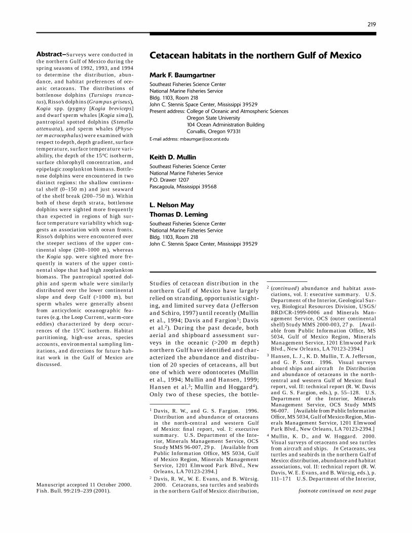
Figure 1Map of shipboard surveys transects conducted by NOAA Ship Oregon II in the spring seasons of 1992, 1993, and 1994. Only transects conducted during active searches for cetaceans during adequate sighting conditions are shown. The 200-m and 2000-m isobaths are indicated in gray.

Gulf of Mexico

30°N30°N

28

26

24

22

20

18

98 96 94 92 90 88 86 84 82 80°W


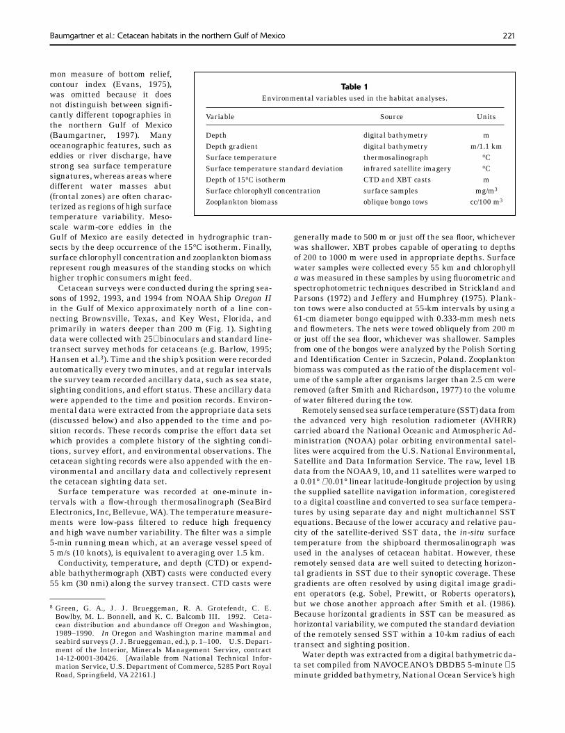
Figure 2Sea surface temperature of the northern Gulf of Mexico derived from remotely sensed AVHRR data collected between 21 and 23 May 1993. Image is a histogram-equalized, warmest-pixel composite of data derived from three satellite passes with some cloud contamination south of 24.5°N and also west of 93°W. CTD and XBT stations are indicated as fi lled circles and the contours represent the depth of the 15°C isotherm computed from the CTD and XBT casts collected between 19 May and 1 June 1993. The line along 27°N indicates the parallel from which data were extracted for Figure 3. The 200-m isobath is shown.

with mesoscale oceanographic features is much larger than these errors and therefore the interpolated fi elds rep-resent these features reasonably well (e.g. Fig. 2).

The base unit of effort for this study was defi ned as 1 km of actively surveyed transect during adequate sighting conditions. To conform to this defi nition, each contiguous transect in the effort data set was broken into 1-km linear sections and all the environmental variables measured along each 1-km section were averaged. This provided a single set of observed environmental variables for each unit of effort. Only those 1-km sections that were actively surveyed (i.e. those where the observers were on-effort) during adequate sighting conditions (defi ned as Beaufort sea states of 3 or less) were used for analysis. Similarly, only those cetacean sightings that occurred while observ-ers were on-effort and in Beaufort sea states of 3 or less were used for analysis. All of the following analyses were conducted on cetacean group sightings and therefore do not account for group size.

Some portions of the described data have been previ-ously published by Davis et al. (1998) and Baumgartner (1997). Davis et al. (1998) examined cetacean habitat in the northwestern Gulf of Mexico with respect to a variety of physical oceanographic and physiographic variables. We have included the sighting data and some of the environ-mental data from that study here (less than 40% of our total data set) to examine cetacean habitat throughout the entire northern Gulf of Mexico with an expanded set of environmental variables and new statistical analyses.

With regard to Risso’s dolphin habitat, we have used the same sighting, depth, and depth gradient data presented in Baumgartner (1997). To these, we have added physical and biological oceanographic variables to test and extend the conclusions of Baumgartner (1997) and to strengthen the univariate and multivariate interspecies comparisons described below.

Analytical methods

The analysis of the sighting and effort data sets was conducted in two parts: 1) univariate and multivariate interspecies comparisons of the environmental variables measured at each cetacean sighting and 2) comparisons of each species’ distribution with respect to the environ-mental variables to that of the effort. The former analysis examined the null hypothesis that each species had simi-lar distributions with respect to each of the environmen-tal variables. This was tested with Mood’s median test (Conover, 1980) and the Kruskal-Wallis test (Sokal and Rohlf, 1981) as nonparametric substitutes for a one-way analysis of variance. Multivariate analysis of variance (MANOVA) and canonical linear discriminant function (LDF) analysis (Huberty, 1994; Johnson, 1998) with rank-transformed environmental variables were used to further examine interspecies differences. These analyses were con-ducted with the CANDISC procedure of the Statistical Analysis System (SAS, 1989), version 6.12. The MANOVA detects species group differences in multivariate space and

30°N

28

26

24

98 96 94 92 90 88 86 84 82°W

32

30

28

26

24

22

20

Sea

Sur

face

Tem

pera

ture

(°C

)


the canonical LDF analysis describes which environmen-tal factors contribute most to these group differences. The canonical LDF analysis is accomplished by fi nding a linear combination of the environmental variables that best dis-criminates between the species groups. These linear com-binations (canonical variables) are then examined by using the LDF structure correlations (Huberty, 1994) to assess their ecological meaning and signifi cance. The structure correlations are essentially the correlations between the canonical variables and the original environmental vari-ables and their interpretation is analogous to the interpre-tation of factor loadings in factor analysis.

The second analysis uses univariate and bivariate chi-squared (χ2) tests, Mann-Whitney tests, Monte Carlo tests, and equal-effort sighting rate distribution plots to deter-mine the specifi c relationships between the distribution of each species and each of the environmental variables. For the χ2 analysis, the effort data were used to compute ex-pected uniform distributions for each species with respect to the individual environmental variables. Classes were chosen such that each contained an equal amount of effort (Kendall and Stuart, 1967). This approach “normalized” the sighting rates by creating class sizes of equal sighting prob-ability based on the effort and guaranteed that the anal-ysis would not be distorted by classes with exceptionally low or high amounts of effort. For a complete description of the methods used to compute the uniform distribution, see Baumgartner (1997). The actual distributions were then compared with the predicted uniform distributions by us-ing the χ2 statistic. Equal-effort sighting rate distribution plots were constructed directly from the contingency tables used in the χ2 analyses. In some cases, the sample size was lower than the minimum required for a conservative χ2 test (n=25), therefore the species’ and effort distributions were compared by using a Mann-Whitney test.

Of the fi ve species examined here, each had a distribu-tion with respect to depth that was signifi cantly different from a uniform distribution. Further analyses with Monte Carlo (randomization) tests were conducted to determine if the distribution of a particular species with respect to the other environmental variables was an artifact of that spe-cies’ distribution with depth. For example, consider a hypo-thetical species that is only found on the continental shelf. The continental shelf in the northern Gulf of Mexico is char-acterized by low depth gradients, whereas the continental slope has high depth gradients and the abyssal plains of the deep Gulf have low depth gradients. Because this species occurs on the continental shelf, it would have distributions with respect to both depth and depth gradient that were signifi cantly different from a uniform distribution. Howev-er, this species’ distribution with respect to depth gradient is merely an artifact of its distribution with respect to depth because of a correspondence between shallow depths and low depth gradients over the continental shelf.

The Monte Carlo tests consisted of randomly choosing n transect sections from the effort data set that had the same depth distribution as the n sightings of the species of interest. These transect sections represent n “virtual” cetacean sightings that have the same depth distribution as the species of interest but have a random distribution

with respect to all of the other environmental variables. A χ2 analysis was then conducted to determine if the dis-tribution of the “virtual” sightings with respect to the par-ticular environmental variable of interest (e.g. depth gra-dient in the example above) was different from a uniform distribution predicted by the effort. The process of choos-ing n “virtual” sightings and of conducting the χ2 analysis was performed 10,000 times. The proportion of the result-ing 10,000 χ2 statistics that exceeded the χ2 statistic as-sociated with the species’ actual distribution with respect to the environmental variable of interest was considered a P-value. This P-value represented the probability that the actual χ2 statistic could have been observed by chance and was used to test the null hypothesis that the species’ distribution with respect to the environmental variable of interest was the same as a uniform distribution given its distribution with respect to depth.

Results

NOAA Ship Oregon II completed 113 days of effort during the spring surveys from 1992 to 1994 and sampled the entire oceanic northern Gulf of Mexico once each year. A total of 9101 1-km transect sections (units of effort) were completed during adequate sighting conditions. The amount of environmental data available for each transect section was dependent on survey design, on instrument availability and performance, and, in the case of the re -motely sensed sea surface temperature variability, on sat-ellite orbital parameters and cloud conditions (Table 2).

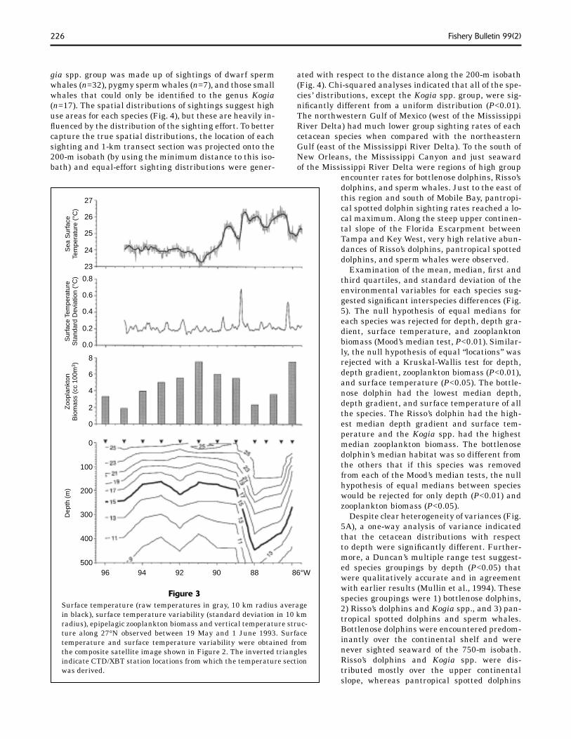
The Loop Current penetrated into the eastern Gulf to at least 27.5°N during each of the surveys and warm-core eddies could usually be found in the central and western Gulf (Fargion et al.10). Both the Loop Current and the warm-core eddies were often accompanied by cold-core fea-tures at their peripheries. Examples of the major oceano-graphic features of the northern Gulf are shown in the composite AVHRR sea surface temperature image and the contoured depth of the 15°C isotherm (Fig. 2). The Loop Current is easily identifi able as the broad region in the eastern Gulf where the 15°C isotherm was at depths be-low 250 to 300 m and sea surface temperatures reached a local maximum. The remnants of a warm-core eddy (Eddy V) are evident in the northwestern Gulf centered at about 27.0°N, 95.5°W (Jockens et al., 1994; Fargion et al.10). Warm-core features like the Loop Current were characterized by depressed isotherms and were often ac-companied by warm surface temperatures and low zoo-plankton biomass (Fig. 3). Surface temperature gradients were high at the edge of these mesoscale features when

10 Fargion, G. S., L. N. May, T. D. Leming, and C. Schroeder. 1996.Oceanographic surveys. In Distribution and abundance of cetaceans in the north-central and western Gulf of Mexico: fi nal report, vol.II: technical report (R.W. Davis and G.S. Far-gion, eds.), p. 207–269. U.S. Department of the Interior, Miner-als Management Service, OCS Study MMS 96-007. [Available from Public Information Offi ce, MS 5034, Gulf of Mexico Region, Minerals Management Service, 1201 Elmwood Park Blvd., New Orleans, LA 70123-2394.]


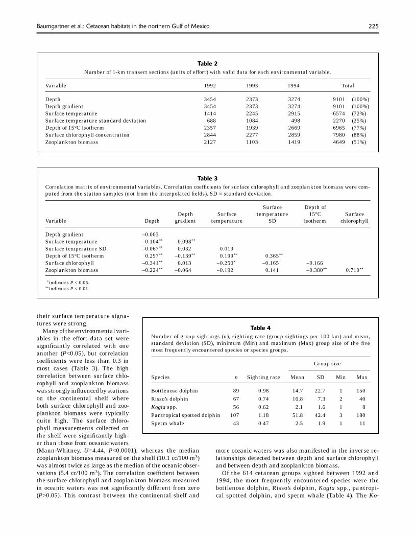
Table 2Number of 1-km transect sections (units of effort) with valid data for each environmental variable.

Variable 1992 1993 1994 Total

Depth 3454 2373 3274 9101 (100%)Depth gradient 3454 2373 3274 9101 (100%)Surface temperature 1414 2245 2915 6574 (72%)Surface temperature standard deviation 688 1084 498 2270 (25%)Depth of 15°C isotherm 2357 1939 2669 6965 (77%)Surface chlorophyll concentration 2844 2277 2859 7980 (88%)Zooplankton biomass 2127 1103 1419 4649 (51%)

Table 3Correlation matrix of environmental variables. Correlation coeffi cients for surface chlorophyll and zooplankton biomass were com-puted from the station samples (not from the interpolated fi elds). SD = standard deviation.

Surface Depth of Depth Surface temperature 15°C SurfaceVariable Depth gradient temperature SD isotherm chlorophyll

Depth gradient –0.003Surface temperature 0.104** 0.098** Surface temperature SD –0.067** 0.032 0.019 Depth of 15°C isotherm 0.297** –0.139** 0.199** 0.365** Surface chlorophyll –0.341** 0.013 –0.250* –0.165 –0.166 Zooplankton biomass –0.224** –0.064 –0.192 0.141 –0.380** 0.710**

** indicates P < 0.05.** indicates P < 0.01.

their surface temperature signa-tures were strong.

Many of the environmental vari-ables in the effort data set were signifi cantly correlated with one another (P<0.05), but correlation coeffi cients were less than 0.3 in most cases (Table 3). The high correlation between surface chlo-rophyll and zooplankton biomass was strongly infl uenced by stations on the continental shelf where both surface chlorophyll and zoo-plankton biomass were typically quite high. The surface chloro-phyll measurements collected on the shelf were signifi cantly high-er than those from oceanic waters

Table 4Number of group sightings (n), sighting rate (group sightings per 100 km) and mean, standard deviation (SD), minimum (Min) and maximum (Max) group size of the fi ve most frequently encountered species or species groups.

Group size

Species n Sighting rate Mean SD Min Max

Bottlenose dolphin 89 0.98 14.7 22.7 1 150Risso’s dolphin 67 0.74 10.8 7.3 2 40Kogia spp. 56 0.62 2.1 1.6 1 8Pantropical spotted dolphin 107 1.18 51.8 42.4 3 180Sperm whale 43 0.47 2.5 1.9 1 11

(Mann-Whitney, U=4.44, P<0.0001), whereas the median zooplankton biomass measured on the shelf (10.1 cc/100 m3) was almost twice as large as the median of the oceanic obser-vations (5.4 cc/100 m3). The correlation coeffi cient between the surface chlorophyll and zooplankton biomass measured in oceanic waters was not signifi cantly different from zero (P>0.05). This contrast between the continental shelf and

more oceanic waters was also manifested in the inverse re-lationships detected between depth and surface chlorophyll and between depth and zooplankton biomass.

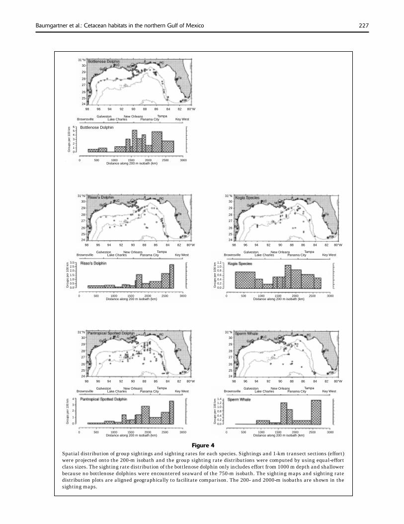
Of the 614 cetacean groups sighted between 1992 and 1994, the most frequently encountered species were the bottlenose dolphin, Risso’s dolphin, Kogia spp., pantropi-cal spotted dolphin, and sperm whale (Table 4). The Ko-


gia spp. group was made up of sightings of dwarf sperm whales (n=32), pygmy sperm whales (n=7), and those small whales that could only be identifi ed to the genus Kogia (n=17). The spatial distributions of sightings suggest high use areas for each species (Fig. 4), but these are heavily in-fl uenced by the distribution of the sighting effort. To better capture the true spatial distributions, the location of each sighting and 1-km transect section was projected onto the 200-m isobath (by using the minimum distance to this iso-bath) and equal-effort sighting distributions were gener-

ated with respect to the distance along the 200-m isobath (Fig. 4). Chi-squared analyses indicated that all of the spe-cies’ distributions, except the Kogia spp. group, were sig-nifi cantly different from a uniform distribution (P<0.01). The northwestern Gulf of Mexico (west of the Mississippi River Delta) had much lower group sighting rates of each cetacean species when compared with the northeastern Gulf (east of the Mississippi River Delta). To the south of New Orleans, the Mississippi Canyon and just seaward of the Mississippi River Delta were regions of high group

encounter rates for bottlenose dolphins, Risso’s dolphins, and sperm whales. Just to the east of this region and south of Mobile Bay, pantropi-cal spotted dolphin sighting rates reached a lo-cal maximum. Along the steep upper continen-tal slope of the Florida Escarpment between Tampa and Key West, very high relative abun-dances of Risso’s dolphins, pantropical spotted dolphins, and sperm whales were observed.

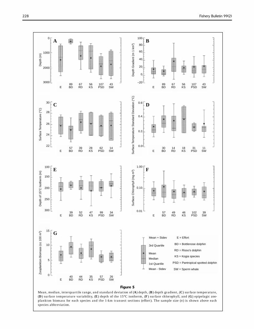
Examination of the mean, median, fi rst and third quartiles, and standard deviation of the environmental variables for each species sug-gested signifi cant interspecies differences (Fig. 5). The null hypothesis of equal medians for each species was rejected for depth, depth gra-dient, surface temperature, and zooplankton biomass (Mood’s median test, P<0.01). Similar-ly, the null hypothesis of equal “locations” was rejected with a Kruskal-Wallis test for depth, depth gradient, zooplankton biomass (P<0.01), and surface temperature (P<0.05). The bottle-nose dolphin had the lowest median depth, depth gradient, and surface temperature of all the species. The Risso’s dolphin had the high-est median depth gradient and surface tem-perature and the Kogia spp. had the highest median zooplankton biomass. The bottlenose dolphin’s median habitat was so different from the others that if this species was removed from each of the Mood’s median tests, the null hypothesis of equal medians between species would be rejected for only depth (P<0.01) and zooplankton biomass (P<0.05).

Despite clear heterogeneity of variances (Fig. 5A), a one-way analysis of variance indicated that the cetacean distributions with respect to depth were signifi cantly different. Further-more, a Duncan’s multiple range test suggest-ed species groupings by depth (P<0.05) that were qualitatively accurate and in agreement with earlier results (Mullin et al., 1994). These species groupings were 1) bottlenose dolphins, 2) Risso’s dolphins and Kogia spp., and 3) pan-tropical spotted dolphins and sperm whales. Bottlenose dolphins were encountered predom-inantly over the continental shelf and were never sighted seaward of the 750-m isobath. Risso’s dolphins and Kogia spp. were dis-tributed mostly over the upper continental slope, whereas pantropical spotted dolphins

Figure 3Surface temperature (raw temperatures in gray, 10 km radius average in black), surface temperature variability (standard deviation in 10 km radius), epipelagic zooplankton biomass and vertical temperature struc-ture along 27°N observed between 19 May and 1 June 1993. Surface temperature and surface temperature variability were obtained from the composite satellite image shown in Figure 2. The inverted triangles indicate CTD/XBT station locations from which the temperature section was derived.

Sea

Sur

face

Tem

pera

ture

(°C

)S

urfa

ce T

empe

ratu

reS

tand

ard

Dev

iatio

n (°

C)

Zoo

plan

kton

Bio

mas

s (c

c 10

0m3 )

Dep

th (

m)

27

26

25

24

23

0.8

0.6

0.4

0.2

0.0

8

6

4

2

0

0

100

200

300

400

50096 94 92 90 88 86°W


Figure 4Spatial distribution of group sightings and sighting rates for each species. Sightings and 1-km transect sections (effort) were projected onto the 200-m isobath and the group sighting rate distributions were computed by using equal-effort class sizes. The sighting rate distribution of the bottlenose dolphin only includes effort from 1000 m depth and shallower because no bottlenose dolphins were encountered seaward of the 750-m isobath. The sighting maps and sighting rate distribution plots are aligned geographically to facilitate comparison. The 200- and 2000-m isobaths are shown in the sighting maps.

31°N

30

29

28

27

26

25

24

98 96 94 92 90 88 86 84 82 80°W

BrownsvilleGalveston

Lake CharlesNew Orleans Tampa

Key WestPanama City

Bottlenose Dolphin

Gro

ups

per

100

km

Distance along 200 m isobath (km)

654

3

210

0 500 1000 1500 2000 2500 3000

31°N

30

29

28

27

26

25

24

98 96 94 92 90 88 86 84 82 80°W



Key WestPanama City


3.02.52.0

1.5

1.00.50.0

0 500 1000 1500 2000 2500 3000

Gro

ups

per

100

km

31°N

30

29

28

27

26

25

24

98 96 94 92 90 88 86 84 82 80°W



Key WestPanama City


1.21.00.8

0.6

0.40.20.0

0 500 1000 1500 2000 2500 3000

Gro

ups

per

100

km

31°N

30

29

28

27

26

25

24

98 96 94 92 90 88 86 84 82 80°W



Key WestPanama City


4

3

2

1

0

0 500 1000 1500 2000 2500 3000

Gro

ups

per

100

km

31°N

30

29

28

27

26

25

24

98 96 94 92 90 88 86 84 82 80°W



Key WestPanama City


1.41.21.0

0.8

0.40.20.0

0 500 1000 1500 2000 2500 3000

Gro

ups

per

100

km


Figure 5Mean, median, interquartile range, and standard deviation of (A) depth, (B) depth gradient, (C) surface temperature, (D) surface temperature variability, (E) depth of the 15°C isotherm, (F) surface chlorophyll, and (G) epipelagic zoo-plankton biomass for each species and the 1-km transect sections (effort). The sample size (n) is shown above each species abbreviation.

A B

C D

E F

G

Sur

face

Tem

pera

ture

(°C

)

30

1000

2000

3000

E89BD

56KS

107PSD

67RD

43SW E

89BD

56KS

107PSD

67RD

43SW

E57BD

28KS

62PSD

39RD

14SW E

30BD

18KS

31PSD

14RD

11SW

E39BD

47KS

99PSD

52RD

34SW E

57BD

46KS

102PSD

49RD

39SW

E40BD

35KS

57PSD

44RD

26SW

Dep

th o

f 15°

C Is

othe

rm (

m)

100

Zoo

plan

kton

Bio

mas

s (c

c 10

0 m

3 ) 15

Dep

th (

m)

0

Dep

th G

radi

ent (

m 1

km

3 )

100

Sur

face

Tem

pera

ture

Sta

ndar

d D

evia

tion

(°C

)

0.6

Sur

face

Chl

orop

hyll

(mg

m3 )

1.00

0.10

0.01

0.4

0.2

0.0

80

60

40

20

0

–20

28

26

24

22

150

200

250

300

10

5

0

Mean + Stdev

3rd Quartile

Mean

Median

1st Quartile

Mean - Stdev

E = Effort

BD = Bottlenose dolphin

RD = Risso’s dolphin

KS = Kogia species

PSD = Pantropical spotted dolphin

SW = Sperm whale


and sperm whales had distributions that extended from the upper continental slope to the deep Gulf. Mann-Whit-ney tests between Risso’s dolphins and Kogia spp. for each of the environmental variables indicated that only their distributions with respect to depth gradient (U=2.12, P<0.05) and zooplankton biomass (U=1.69, P<0.05) were signifi cantly different. Similar tests between pantropical spotted dolphins and sperm whales indicated that their distributions with respect to the depth of the 15°C iso-therm (U=2.26, P<0.05) alone were signifi cantly different.

Differences between species were also detected with MANOVA and canonical linear discriminant function anal-ysis. Unfortunately, low sample size for both sea surface temperature and sea surface temperature variability pre-cluded their use in the multivariate analyses. Of the re-maining variables, the sample sizes for each species were as follows: bottlenose dolphins (n=18), Risso’s dolphins (n=35), Kogia spp. (n=25), pantropical spotted dolphins (n=51), and sperm whales (n=19). The null hypothesis of equal mean vectors was rejected in the MANOVA (Wilks’ λ=0.446, P<0.0001). The fi rst two canonical variables in the canonical LDF analysis accounted for 94.5% of the

total variability, and likelihood ratio tests indicated that only the fi rst two canonical variables were signifi cant (P<0.01 for each). The structure correlations indicated that low depths and high zooplankton biomass were associated with positive values of the fi rst canonical variable, where-as shallow occurrences of the depth of the 15°C isotherm and low surface chlorophyll concentration were associated with positive values of the second canonical variable (Fig. 6A). The separation between groups along canonical axis 1 supports the importance of depth in habitat partition-ing in the northern Gulf of Mexico. The signifi cance of zoo-plankton biomass in this fi rst canonical variable was due to the inclusion of the bottlenose dolphin in the analysis and the presence of high zooplankton biomass on the con-tinental shelf. Note that the bottlenose dolphin was clearly separated from the other species along canonical axis 1 and the sperm whale was separated from the other species on both canonical axes.

Because inclusion of the bottlenose dolphin strongly infl uenced the results of the multivariate analysis, a sec-ond analysis was conducted for just the oceanic species. The null hypothesis of equal mean vectors was rejected

Figure 6Means and interquartile ranges (error bars) of the canonical linear discriminant function variables for (A) all species and (B) all species except the bottlenose dolphin. The structure correlations associated with each canonical axis represent the approximate correlations between the canonical variables and depth (DP), depth gradient (DPG), depth of the 15°C isotherm (D15C), surface chlorophyll concentration (CHL), and epipelagic zooplankton biomass (PL). Species abbreviations are the same as those shown in Figure 5.

3

2

1

0

–1

–2

–2 –1 0 1 2 3

2

1

0

–1

–2

–2 –1 0 1 2

1.00.5

0.0

–0.5–1.0

Can

onic

al A

xis

1S

truc

ture

Cor

r. 1.00.5

0.0

–0.5–1.0

Can

onic

al A

xis

2S

truc

ture

Cor

r. 1.00.5

0.0

–0.5–1.0

Can

onic

al A

xis

1S

truc

ture

Cor

r. 1.00.5

0.0

–0.5–1.0

Can

onic

al A

xis

2S

truc

ture

Cor

r.

DP D15C PLDPG CHL

DP D15C PLDPG CHL

DP D15C PLDPG CHL

DP D15C PLDPG CHL

Can

onic

al a

xis

2

Canonical axis 1


again in the MANOVA (Wilks’ λ=0.675, P<0.0001). The fi rst two canonical variables in the canonical LDF analysis accounted for 94.2% of the total variability, and likelihood ratio tests indicated that only these fi rst two canonical variables were signifi cant (P<0.0001 for the fi rst, P<0.05 for the second). The correlation structure suggested that high values of zooplankton biomass and deep occurrences of the depth of the 15°C isotherm were associated with positive values of the fi rst canonical variable, whereas high values for depth and surface chlorophyll were associ-ated with positive values of the second canonical variable (Fig. 6B). Although there seems to be considerable overlap between the Risso’s dolphin, pantropical spotted dolphin, and Kogia spp. in the canonical space, the sperm whale is separated from the other species primarily along canoni-cal axis 1 (Fig. 6B).

Bottlenose dolphin

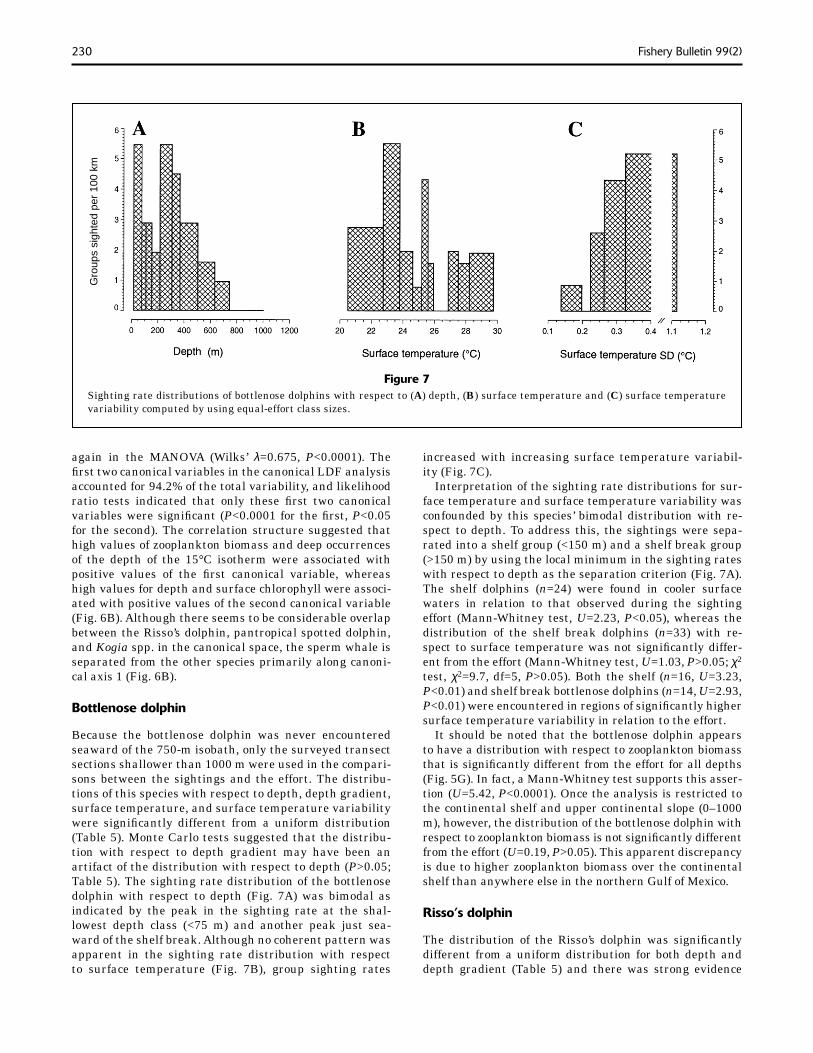
Because the bottlenose dolphin was never encountered seaward of the 750-m isobath, only the surveyed transect sections shallower than 1000 m were used in the compari-sons between the sightings and the effort. The distribu-tions of this species with respect to depth, depth gradient, surface temperature, and surface temperature variability were signifi cantly different from a uniform distribution (Table 5). Monte Carlo tests suggested that the distribu-tion with respect to depth gradient may have been an artifact of the distribution with respect to depth (P>0.05; Table 5). The sighting rate distribution of the bottlenose dolphin with respect to depth (Fig. 7A) was bimodal as indicated by the peak in the sighting rate at the shal-lowest depth class (<75 m) and another peak just sea-ward of the shelf break. Although no coherent pattern was apparent in the sighting rate distribution with respect to surface temperature (Fig. 7B), group sighting rates

Figure 7Sighting rate distributions of bottlenose dolphins with respect to (A) depth, (B) surface temperature and (C) surface temperature variability computed by using equal-effort class sizes.

increased with increasing surface temperature variabil-ity (Fig. 7C).

Interpretation of the sighting rate distributions for sur-face temperature and surface temperature variability was confounded by this species’ bimodal distribution with re-spect to depth. To address this, the sightings were sepa-rated into a shelf group (<150 m) and a shelf break group (>150 m) by using the local minimum in the sighting rates with respect to depth as the separation criterion (Fig. 7A). The shelf dolphins (n=24) were found in cooler surface waters in relation to that observed during the sighting effort (Mann-Whitney test, U=2.23, P<0.05), whereas the distribution of the shelf break dolphins (n=33) with re-spect to surface temperature was not signifi cantly differ-ent from the effort (Mann-Whitney test, U=1.03, P>0.05; χ2 test, χ2=9.7, df=5, P>0.05). Both the shelf (n=16, U=3.23, P<0.01) and shelf break bottlenose dolphins (n=14, U=2.93, P<0.01) were encountered in regions of signifi cantly higher surface temperature variability in relation to the effort.

It should be noted that the bottlenose dolphin appears to have a distribution with respect to zooplankton biomass that is signifi cantly different from the effort for all depths (Fig. 5G). In fact, a Mann-Whitney test supports this asser-tion (U=5.42, P<0.0001). Once the analysis is restricted to the continental shelf and upper continental slope (0–1000 m), however, the distribution of the bottlenose dolphin with respect to zooplankton biomass is not signifi cantly different from the effort (U=0.19, P>0.05). This apparent discrepancy is due to higher zooplankton biomass over the continental shelf than anywhere else in the northern Gulf of Mexico.

Risso’s dolphin

The distribution of the Risso’s dolphin was signifi cantly different from a uniform distribution for both depth and depth gradient (Table 5) and there was strong evidence

Gro

ups

sigh

ted

per

100

km


Table 5Results for univariate χ2, Mann-Whitney, and Monte Carlo tests. Values of 0.0000 for P indicate P < 0.0001.

χ2 test Mann-Whitney Monte Carlo

n χ2 df P U P P

Bottlenose dolphin Depth 89 57.6 11 0.0000** — Depth gradient 89 23.1 11 0.0174* 0.7474 Surface temperature 57 26.8 9 0.0015** 0.0224*

Surface temperature standard deviation 30 17.3 4 0.0017** 0.0018**

Depth of 15°C isotherm 39 6.0 6 0.4184 0.4909 Surface chlorophyll 57 12.2 9 0.1999 0.4095 Zooplankton biomass 40 1.9 6 0.9268 0.9720

Risso’s dolphin Depth 67 53.9 12 0.0000** — Depth gradient 67 57.4 12 0.0000** 0.0000**

Surface temperature 39 9.9 6 0.1296 0.1527 Surface temperature standard deviation 14 1.69 0.0456*

Depth of 15°C isotherm 52 16.3 9 0.0603 0.0971 Surface chlorophyll 49 9.2 8 0.3232 0.3227 Zooplankton biomass 44 7.3 7 0.3970 0.7056

Kogia spp. Depth 56 42.6 9 0.0000** — Depth gradient 56 20.4 9 0.0155* 0.0690 Surface temperature 28 4.8 4 0.3038 0.3540 Surface temperature standard deviation 18 1.98 0.0238*

Depth of 15°C isotherm 47 7.2 8 0.5125 0.5371 Surface chlorophyll 46 3.4 7 0.8441 0.8560 Zooplankton biomass 35 31.6 5 0.0000** 0.0014**

Pantropical spotted dolphin Depth 107 50.6 11 0.0000** — Depth gradient 107 25.1 11 0.0088** 0.0687 Surface temperature 62 13.5 11 0.2614 0.3616 Surface temperature standard deviation 31 7.5 4 0.1096 0.1148 Depth of 15°C isotherm 99 19.1 11 0.0593 0.0748 Surface chlorophyll 102 20.6 11 0.0380* 0.0985 Zooplankton biomass 57 16.4 9 0.0588 0.3522

Sperm whale Depth 43 14.5 7 0.0431* — Depth gradient 43 13.7 7 0.0566 0.0965 Surface temperature 14 0.27 0.3921 Surface temperature standard deviation 11 1.14 0.1268 Depth of 15°C isotherm 34 11.0 5 0.0508 0.0388*

Surface chlorophyll 39 11.5 6 0.0741 0.0749 Zooplankton biomass 26 3.5 4 0.4729 0.7053

** indicates P < 0.05.** indicates P < 0.01.

that the distribution with respect to depth gradient was not an artifact of the depth distribution (P<0.0001). The distribution with respect to surface temperature variabil-ity was signifi cantly different from the effort (P<0.05; Table 5) and surface temperature variability at Risso’s

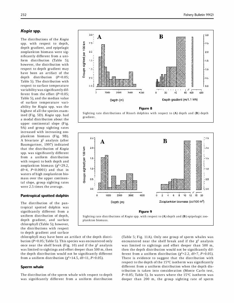
dolphin sightings was generally higher than the effort (Fig. 5D). The sighting rate distribution with respect to depth was modal about the upper continental slope (Fig. 8A), whereas group sighting rates increased with increas-ing depth gradient (Fig. 8B).


Kogia spp.

The distributions of the Kogia spp. with respect to depth, depth gradient, and epipelagic zooplankton biomass were sig-nifi cantly different from a uni-form distribution (Table 5); however, the distribution with respect to depth gradient may have been an artifact of the depth distribution (P>0.05; Table 5). The distribution with respect to surface temperature variability was signifi cantly dif-ferent from the effort (P<0.05; Table 5), and the median value of surface temperature vari-ability for Kogia spp. was the highest of all the species exam-ined (Fig. 5D). Kogia spp. had a modal distribution about the upper continental slope (Fig. 9A) and group sighting rates increased with increasing zoo-plankton biomass (Fig. 9B). A bivariate χ2 analysis (after Baumgartner, 1997) indicated that the distribution of Kogia spp. was signifi cantly different from a uniform distribution with respect to both depth and zooplankton biomass (χ2=29.2, df=4, P<0.0001) and that in waters of high zooplankton bio-mass over the upper continen-tal slope, group sighting rates were 2.5 times the average.

Pantropical spotted dolphin

The distribution of the pan-tropical spotted dolphin was signifi cantly different from a uniform distribution of depth, depth gradient, and surface chlorophyll (Table 5); however, the distributions with respect to depth gradient and surface

Figure 8Sighting rate distributions of Risso’s dolphins with respect to (A) depth and (B) depth gradient.

Figure 9Sighting rate distributions of Kogia spp. with respect to (A) depth and (B) epipelagic zoo-plankton biomass.

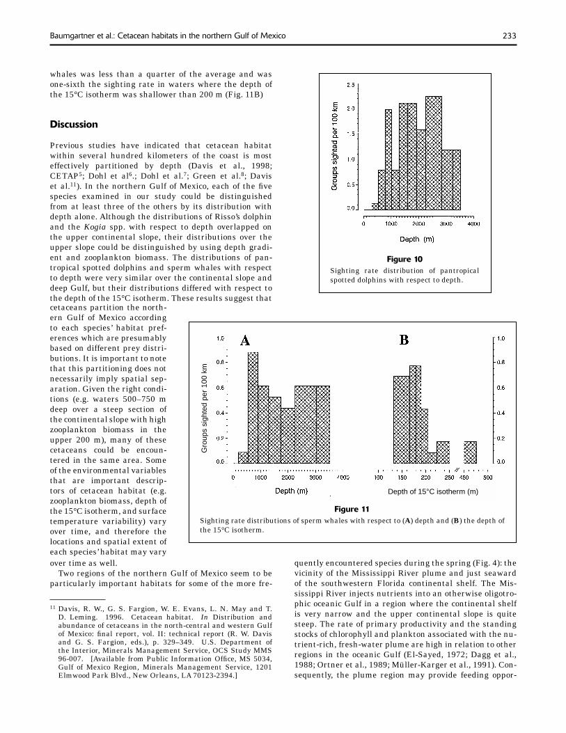
chlorophyll may have been an artifact of the depth distri-bution (P>0.05; Table 5). This species was encountered only once near the shelf break (Fig. 10) and if the χ2 analysis was limited to sightings and effort deeper than 500 m, then the depth distribution would not be signifi cantly different from a uniform distribution (χ2=14.5, df=11, P>0.05).

Sperm whale

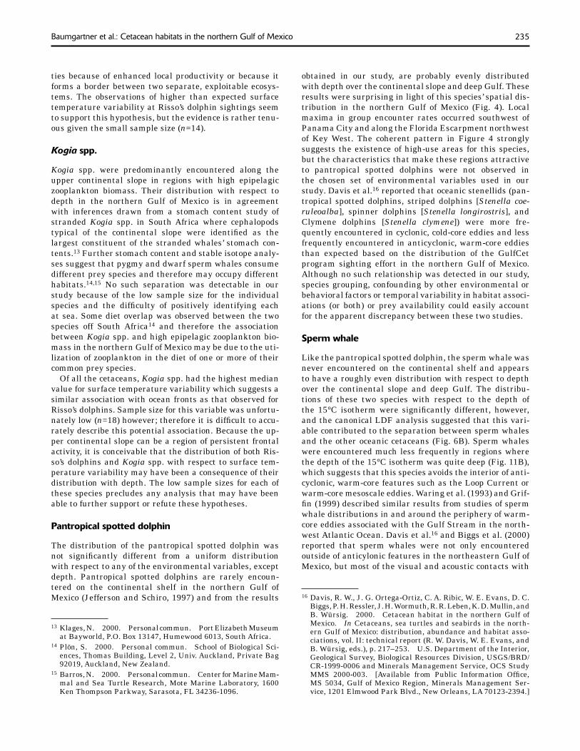
The distribution of the sperm whale with respect to depth was signifi cantly different from a uniform distribution

(Table 5; Fig. 11A). Only one group of sperm whales was encountered near the shelf break and if the χ2 analysis was limited to sightings and effort deeper than 500 m, then the depth distribution would not be signifi cantly dif-ferent from a uniform distribution (χ2=2.2, df=7, P>0.05). There is evidence to suggest that the distribution with respect to the depth of the 15°C isotherm was signifi cantly different from a uniform distribution when the depth dis-tribution is taken into consideration (Monte Carlo test, P<0.05; Table 5). In waters where the 15°C isotherm was deeper than 200 m, the group sighting rate of sperm


Figure 11Sighting rate distributions of sperm whales with respect to (A) depth and (B) the depth of the 15°C isotherm.

whales was less than a quarter of the average and was one-sixth the sighting rate in waters where the depth of the 15°C isotherm was shallower than 200 m (Fig. 11B)

Discussion

Previous studies have indicated that cetacean habitat within several hundred kilometers of the coast is most effectively partitioned by depth (Davis et al., 1998; CETAP5; Dohl et al6.; Dohl et al.7; Green et al.8; Davis et al.11). In the northern Gulf of Mexico, each of the fi ve species examined in our study could be distinguished from at least three of the others by its distribution with depth alone. Although the distributions of Risso’s dolphin and the Kogia spp. with respect to depth overlapped on the upper continental slope, their distributions over the upper slope could be distinguished by using depth gradi-ent and zooplankton biomass. The distributions of pan-tropical spotted dolphins and sperm whales with respect to depth were very similar over the continental slope and deep Gulf, but their distributions differed with respect to the depth of the 15°C isotherm. These results suggest that cetaceans partition the north-ern Gulf of Mexico according to each species’ habitat pref-erences which are presumably based on different prey distri-butions. It is important to note that this partitioning does not necessarily imply spatial sep-aration. Given the right condi-tions (e.g. waters 500–750 m deep over a steep section of the continental slope with high zooplankton biomass in the upper 200 m), many of these cetaceans could be encoun-tered in the same area. Some of the environmental variables that are important descrip-tors of cetacean habitat (e.g. zooplankton biomass, depth of the 15°C isotherm, and surface temperature variability) vary over time, and therefore the locations and spatial extent of each species’ habitat may vary

quently encountered species during the spring (Fig. 4): the vicinity of the Mississippi River plume and just seaward of the southwestern Florida continental shelf. The Mis-sissippi River injects nutrients into an otherwise oligotro-phic oceanic Gulf in a region where the continental shelf is very narrow and the upper continental slope is quite steep. The rate of primary productivity and the standing stocks of chlorophyll and plankton associated with the nu-trient-rich, fresh-water plume are high in relation to other regions in the oceanic Gulf (El-Sayed, 1972; Dagg et al., 1988; Ortner et al., 1989; Müller-Karger et al., 1991). Con-sequently, the plume region may provide feeding oppor-

11 Davis, R. W., G. S. Fargion, W. E. Evans, L. N. May and T. D. Leming. 1996. Cetacean habitat. In Distribution and abundance of cetaceans in the north-central and western Gulf of Mexico: fi nal report, vol. II: technical report (R. W. Davis and G. S. Fargion, eds.), p. 329–349. U.S. Department of the Interior, Minerals Management Service, OCS Study MMS 96-007. [Available from Public Information Offi ce, MS 5034, Gulf of Mexico Region, Minerals Management Service, 1201 Elmwood Park Blvd., New Orleans, LA 70123-2394.]

over time as well.Two regions of the northern Gulf of Mexico seem to be

particularly important habitats for some of the more fre-

Figure 10Sighting rate distribution of pantropical spotted dolphins with respect to depth.

Gro

ups

sigh

ted

per

100

km

Depth of 15°C isotherm (m)


tunities for cetaceans through local trophic interactions. Likewise, the area west of the southwestern Florida shelf break may be another region of high productivity. The physical oceanography of this region is characterized by the formation of a cyclonic meander or eddy in the spring between the Loop Current to the west and the steep Flor-ida Escarpment to the east (Cochrane, 1972; Vukovich et al., 1979; Vukovich and Maul, 1985). Maul et al. (1984) ob-served that bluefi n tuna catch per unit of effort inside a cold-core meander in this region was three times higher than in the central Gulf the previous year. Between 83– 86°W and 24– 27°N in oceanic waters, the sighting rates of Risso’s dolphins, pantropical spotted dolphins, and sperm whales were 3.8, 2.6, and 2.8 times higher than the aver-age sighting rate and 4.9, 3.0, and 3.3 times higher than the sighting rate outside of this region, respectively.

Bottlenose dolphin

The bottlenose dolphin’s distribution in the northern Gulf of Mexico is markedly different from the other species examined in our study. This species and the Atlantic spot-ted dolphin are the only cetaceans that are routinely encountered on the continental shelf (Fritts et al., 1983; Mullin et al., 1994; Jefferson and Schiro, 1997; Hansen et al.3). Caution is warranted when interpreting the bimodal distribution of bottlenose dolphin sighting rates with respect to depth (Fig. 7A). Effort on the continental shelf was neither extensive nor distributed uniformly through-out the northern Gulf. During the CETAP study (Kenney, 1990; CETAP5), a distinct bimodal distribution of bottle-nose dolphins was observed north of Cape Hatteras. Bot-tlenose dolphins were concentrated during warm months in waters less than 25 m and year round near the 1000-m isobath and some groups were sighted in waters as deep as 4712 m (CETAP5). This bimodal distribution is sugges-tive of the inshore (coastal) and offshore forms of bottle-nose dolphins described by others (Norris and Prescott, 1961; Walker, 1975; Leatherwood and Reeves, 1982; Shane et al., 1986; Kenney, 1990; Walker12) and supported by mitochondrial DNA (Dowling and Brown, 1993; Curry and Smith, 1997), hematological (Duffi eld et al., 1983; Hersh and Duffi eld, 1990), and morphological (Hersh and Duff-ield, 1990) evidence. The spatial distribution of bottlenose dolphin group sightings from aerial surveys on the conti-nental shelf of the Gulf of Mexico (Blaylock et al., 1995) and off the southeast U.S. coast south of Cape Hatteras (Blaylock and Hoggard, 1994), however, was not character-ized by any large-scale discontinuities in bottlenose dol-phin distribution similar to those observed north of Cape Hatteras.

The shelf bottlenose dolphins were found in regions with cooler than expected surface waters and high surface tem-

perature variability. These oceanographic characteristics are consistent with the cool and fresh water side of fronts associated with river plumes and, indeed, sighting rates of the shelf bottlenose dolphins were particularly high near the Mississippi River Delta. Sighting rates of the shelf break bottlenose dolphins were more evenly distributed in the central and eastern Gulf and the high surface temper-ature variability observed near these dolphins suggests a potential association with shelf break fronts.

Risso’s dolphin

Baumgartner (1997) examined the same 1992–94 spring cruise data used in our study with the intent of defi ning Risso’s dolphin habitat in terms of the physiography of the northern Gulf of Mexico. Using both univariate and bivariate analyses, he determined that the sighting rate of Risso’s dolphin groups between the 350- and 975-m iso-baths and in depth gradients exceeding 24 m per 1.1 km was nearly 5 times the average. Of the groups encountered outside this region, 40% were sighted within 5 km of it. Aerial survey data collected during all seasons between 1992 and 1994 were used to independently assess this habitat model. Sighting rates from these surveys were nearly 6 times the average inside this core habitat, and of the groups encountered outside of this region, 73% were sighted within 5 km of it.

The distribution of Risso’s dolphin along the continen-tal slope has been noted in several studies (Würtz et al., 1992; CETAP5; Dohl et al.6; Dohl et al.7; Green et al.8; Da-vis et al.11) and some evidence exists to support this spe-cies’ association with the steeper sections of the upper con-tinental slope elsewhere. Off the Oregon and Washington coasts, Green et al.8 observed that Risso’s dolphin encoun-ter rates over the continental slope (200–2000 m) were seven times greater than on the shelf and that the groups sighted on the shelf were very close to the shelf break. Compared with the northern Gulf of Mexico, almost the entire Oregon–Washington continental slope can be con-sidered steep with depth gradients in excess of 22 m per 1.1 km (Fig. 11 in Green et al.8). Dohl et al.7 found a simi-lar distribution off central and northern California, where the majority of Risso’s dolphin sightings were between the 183- and 1830-m (100–1000 fathom) isobaths. As is the case off Oregon and Washington, virtually all of the con-tinental slope off central and northern California can be considered very steep (Fig. 1 in Dohl et al.7). The physiog-raphy of the northwestern Atlantic Ocean is much more like that found in the northern Gulf of Mexico and the CETAP study (Hain et al., 1985; Kenney and Winn, 1986; CETAP5) found Risso’s dolphins concentrated at the shelf break (mode of 478 sightings was 183 m depth) and dis-tributed over the entire continental slope (average of 478 sightings was 1092 m).

Baumgartner (1997) hypothesized that Risso’s dolphins aggregate along the upper continental slope because of the presence of a persistent ocean front separating the rela-tively cool and fresh waters of the continental shelf and the more warm and salty waters of the oceanic Gulf. This shelf break front may provide greater feeding opportuni-

12 Walker, W. A. 1981. Geographical variation in morphology and biology of bottlenose dolphins (Tursiops) in the eastern North Pacifi c. Southwest Fisheries Center Administrative Report LJ-81-03C, 52 p. [Available from Southwest Fisheries Science Center, National Marine Fisheries Service, NOAA, P.O. Box 271, La Jolla, CA 92038.]


ties because of enhanced local productivity or because it forms a border between two separate, exploitable ecosys-tems. The observations of higher than expected surface temperature variability at Risso’s dolphin sightings seem to support this hypothesis, but the evidence is rather tenu-ous given the small sample size (n=14).

Kogia spp.

Kogia spp. were predominantly encountered along the upper continental slope in regions with high epipelagic zooplankton biomass. Their distribution with respect to depth in the northern Gulf of Mexico is in agreement with inferences drawn from a stomach content study of stranded Kogia spp. in South Africa where cephalopods typical of the continental slope were identifi ed as the largest constituent of the stranded whales’ stomach con-tents.13 Further stomach content and stable isotope analy-ses suggest that pygmy and dwarf sperm whales consume different prey species and therefore may occupy different habitats.14,15 No such separation was detectable in our study because of the low sample size for the individual species and the diffi culty of positively identifying each at sea. Some diet overlap was observed between the two species off South Africa14 and therefore the association between Kogia spp. and high epipelagic zooplankton bio-mass in the northern Gulf of Mexico may be due to the uti-lization of zooplankton in the diet of one or more of their common prey species.

Of all the cetaceans, Kogia spp. had the highest median value for surface temperature variability which suggests a similar association with ocean fronts as that observed for Risso’s dolphins. Sample size for this variable was unfortu-nately low (n=18) however; therefore it is diffi cult to accu-rately describe this potential association. Because the up-per continental slope can be a region of persistent frontal activity, it is conceivable that the distribution of both Ris-so’s dolphins and Kogia spp. with respect to surface tem-perature variability may have been a consequence of their distribution with depth. The low sample sizes for each of these species precludes any analysis that may have been able to further support or refute these hypotheses.

Pantropical spotted dolphin

The distribution of the pantropical spotted dolphin was not signifi cantly different from a uniform distribution with respect to any of the environmental variables, except depth. Pantropical spotted dolphins are rarely encoun-tered on the continental shelf in the northern Gulf of Mexico (Jefferson and Schiro, 1997) and from the results

13 Klages, N. 2000. Personal commun. Port Elizabeth Museum at Bayworld, P.O. Box 13147, Humewood 6013, South Africa.

14 Plön, S. 2000. Personal commun. School of Biological Sci-ences, Thomas Building, Level 2, Univ. Auckland, Private Bag 92019, Auckland, New Zealand.

15 Barros, N. 2000. Personal commun. Center for Marine Mam-mal and Sea Turtle Research, Mote Marine Laboratory, 1600 Ken Thompson Parkway, Sarasota, FL 34236-1096.

obtained in our study, are probably evenly distributed with depth over the continental slope and deep Gulf. These results were surprising in light of this species’ spatial dis-tribution in the northern Gulf of Mexico (Fig. 4). Local maxima in group encounter rates occurred southwest of Panama City and along the Florida Escarpment northwest of Key West. The coherent pattern in Figure 4 strongly suggests the existence of high-use areas for this species, but the characteristics that make these regions attractive to pantropical spotted dolphins were not observed in the chosen set of environmental variables used in our study. Davis et al.16 reported that oceanic stenellids (pan-tropical spotted dolphins, striped dolphins [Stenella coe-ruleoalba], spinner dolphins [Stenella longirostris], and Clymene dolphins [Stenella clymene]) were more fre-quently encountered in cyclonic, cold-core eddies and less frequently encountered in anticyclonic, warm-core eddies than expected based on the distribution of the GulfCet program sighting effort in the northern Gulf of Mexico. Although no such relationship was detected in our study, species grouping, confounding by other environmental or behavioral factors or temporal variability in habitat associ-ations (or both) or prey availability could easily account for the apparent discrepancy between these two studies.

Sperm whale

Like the pantropical spotted dolphin, the sperm whale was never encountered on the continental shelf and appears to have a roughly even distribution with respect to depth over the continental slope and deep Gulf. The distribu-tions of these two species with respect to the depth of the 15°C isotherm were signifi cantly different, however, and the canonical LDF analysis suggested that this vari-able contributed to the separation between sperm whales and the other oceanic cetaceans (Fig. 6B). Sperm whales were encountered much less frequently in regions where the depth of the 15°C isotherm was quite deep (Fig. 11B), which suggests that this species avoids the interior of anti-cyclonic, warm-core features such as the Loop Current or warm-core mesoscale eddies. Waring et al. (1993) and Grif-fi n (1999) described similar results from studies of sperm whale distributions in and around the periphery of warm-core eddies associated with the Gulf Stream in the north-west Atlantic Ocean. Davis et al.16 and Biggs et al. (2000) reported that sperm whales were not only encountered outside of anticylonic features in the northeastern Gulf of Mexico, but most of the visual and acoustic contacts with

16 Davis, R. W., J. G. Ortega-Ortiz, C. A. Ribic, W. E. Evans, D. C. Biggs, P. H. Ressler, J. H. Wormuth, R. R. Leben, K. D. Mullin, and B. Würsig. 2000. Cetacean habitat in the northern Gulf of Mexico. In Cetaceans, sea turtles and seabirds in the north-ern Gulf of Mexico: distribution, abundance and habitat asso-ciations, vol. II: technical report (R. W. Davis, W. E. Evans, and B. Würsig, eds.), p. 217–253. U.S. Department of the Interior, Geological Survey, Biological Resources Division, USGS/BRD/CR-1999-0006 and Minerals Management Service, OCS Study MMS 2000-003. [Available from Public Information Offi ce, MS 5034, Gulf of Mexico Region, Minerals Management Ser-vice, 1201 Elmwood Park Blvd., New Orleans, LA 70123-2394.]


sperm whales during the GulfCet II focal cruises were in regions characterized by cyclonic mesoscale features.

Jaquet (1996) reviewed a variety of sperm whale habitat studies that seemed to have contradictory conclusions re-garding the primary oceanographic processes infl uencing sperm whale distribution (namely upwelling and down-welling). Jaquet attributed these discrepancies to a prob-lem of defi ning the appropriate spatial and temporal scales, and she and others illustrated this point by demonstrating a varying but positive correlation between historical sperm whale catches and surface chlorophyll over increasing tem-poral and spatial scales in the equatorial Pacifi c (Jaquet et al., 1996). These results seem to indicate that upwelling, which contributes to increased surface phytoplankton bio-mass, is a predominant factor in infl uencing sperm whale distribution in the equatorial Pacifi c. Historical catches in temperate waters, however, are not at all correlated with surface chlorophyll (see Fig. 1 of Jaquet, 1996 and Fig. 1 of Jaquet et al., 1996) which suggests that other oceano-graphic processes or physiographic infl uences may be im-portant (e.g. downwelling or biological-physical processes associated with continental slopes). At comparatively short time scales and small spatial scales, we found no evidence to suggest a relationship between the distribution of sperm whales and surface chlorophyll in the northern Gulf of Mexico. Even at longer temporal and larger spatial scales, we would expect this same result because the oceanic Gulf is persistently oligotrophic both in time and space (Müller-Karger et al., 1991; Longhurst, 1998).

Berzin (1971) examined harvest records from the world-wide sperm whale fi shery and suggested that sperm whale distribution was closely linked to processes that support-ed the meso- and bathypelagic food webs. Because sperm whales feed almost exclusively on mesopelagic or demer-sal cephalopods (Clarke, 1986, 1996), they probably aggre-gate in areas where these prey are abundant. These deep-water prey species are entirely dependent on the rain of organic matter from the surface for their sustenance and so these species will be found in regions where the export of detritus from the surface is enhanced. This process oc-curs in convergence zones where downwelling forces sur-face biomass and oxygen into the deep ocean, such as in the middle of anticyclonic eddies, at the peripheries of cy-clonic eddies, to the right (left) of surface ocean currents in the northern (southern) hemisphere, in the middle of the large-scale anticyclonic ocean gyres (e.g. the Sargasso Sea), or along fronts where surface water masses abut. The global sperm whale distribution maps provided by Townsend (1935) and Berzin (1971) do indeed suggest that this species was frequently harvested in or near large-scale oceanic convergence zones, especially along the sub-tropical convergence zones and the Antarctic polar front.

The distribution of sperm whales in the northern Gulf of Mexico and northwestern Atlantic Ocean (Waring et al., 1993; Griffi n, 1999) seems contradictory to Berzin’s hy-pothesis, however. Features such as the Loop Current or warm-core eddies rotate anticyclonically and have conver-gent centers in which downwelling occurs. According to Berzin’s hypothesis, the interior of these features would be favorable to sperm whales because of the enhanced export

of surface biomass to the deep ocean and the resultant in-crease in prey species. The interior of anticyclonic eddies in the northern Gulf of Mexico are, however, low in surface zooplankton biomass (Biggs, 1992). Although the rate of detrital export to the deep is enhanced by increased verti-cal velocities within these features, the amount of biomass actually exported may be too small to support large popu-lations of deep-water prey.

Another possible explanation for the distribution of sperm whales with respect to the depth of the 15°C iso-therm is related to the availability of prey. Berzin (1971) characterized cephalopods as thermophilic and thus in-dicated that they are distributed within a narrow range of ocean temperatures according to their species-specifi c thermal requirements or to the thermal requirements of their prey. These requirements not only govern the hori-zontal distribution of cephalopods, but their vertical dis-tribution as well. Because warm-core features are charac-terized by depressed isotherms (e.g. Fig. 3), cephalopods within these features may be hundreds of meters deeper in the water column than in the waters outside these fea-tures. Despite their well-known ability to dive to great depths, foraging continuously at greater depths under warm-core features would be much more energetically ex-pensive than foraging outside these features. Thus, when prey abundance inside and outside of warm-core eddies are equivalent, sperm whales may feed on prey distribut-ed at shallower depths outside of these features to reduce their energy expenditure.

Caveats

It is important to remember that this study was limited to surveys conducted during the spring season. The spa-tial distribution of cetaceans may be different in other sea-sons because the oceanographic conditions of the northern Gulf of Mexico change over the course of the year. The northward penetration of the Loop Current into the Gulf varies on a quasi-annual basis (Vukovich et al., 1979; Stur-ges and Evans, 1983; Vukovich, 1995) and the variability in the position of the Loop Current affects the generation and positions of both anticyclonic and cyclonic eddies. This variability may, in turn, greatly infl uence the productiv-ity and availability of prey species in the eastern Gulf of Mexico. In the northwestern Gulf, the slow march of warm-core eddies from east to west toward the “eddy graveyard” over the continental slope also varies with time and may affect the seasonal distribution of cetaceans. Hansen et al.3 observed seasonal differences in cetacean abundance in the western and central regions of the northern Gulf of Mexico that may have been infl uenced by temporal changes in the local oceanography.

Another potential limitation of our study was the rather coarse environmental sampling. Although the CTD/XBT sampling strategy was suffi cient to identify the large-scale oceanographic features, some of the most biologically sig-nifi cant processes in the oceanic Gulf of Mexico occur on smaller spatial scales. In particular, the outer edge of the Loop Current is frequently a site of upwelling and these divergent features often develop into cyclonic meanders


and eddies at the northern and eastern sides of the Loop Current (Vukovich and Maul, 1985). These cyclonic fea-tures are usually much smaller than the Loop Current itself or the warm-core features of the central and west-ern Gulf (Cochrane, 1972). Along the latitude of 27°N and within 40 km of the Loop Current (near 88.8°W) in late spring, 1993, for instance, the satellite-borne AVHRR de-tected surface temperatures 1.5°C cooler than the Loop Current itself, but the vertical temperature structure, sur-face chlorophyll and zooplankton biomass associated with this narrow feature were not captured because of the coarse sampling strategy (Figs. 2 and 3). The recent Gulf-Cet II program (Davis et al.16) examined cetacean habitat associations in the vicinity of cyclonic-anticyclonic eddy pairs in the northeastern Gulf of Mexico and demonstrat-ed that these mesoscale hydrographic features can indeed infl uence cetacean distribution. In addition to the cyclonic features associated with the Loop Current, the CTD and XBT sampling strategy of our study did not resolve other potentially productive features that occur on smaller spa-tial scales, such as nutrient-rich Mississippi River plume waters entrained at the edge of the Loop Current (Maul, 1977; Müller-Karger et al., 1991) and shelf break fronts.

Future studies of cetacean habitats in the Gulf of Mexi-co should continue to consider these smaller scale features as potential sites of large cetacean aggregations because of their high levels of biological activity. These features could potentially 1) have high rates of primary productiv-ity that is converted into prey biomass over short tempo-ral and spatial scales, 2) concentrate prey through solely physical mechanisms or through physical-biological inter-actions or 3) make local prey more accessible to surface-bound cetaceans. Although investigating these processes is undoubtedly a challenge, it is important to elucidate what processes affect cetacean distribution and at what spatial and temporal scales these processes operate if we are to understand how oceanographic conditions affect ce-tacean ecology.

Acknowledgments

This work was supported by the National Marine Fisher-ies Service’s Marine Mammal Program. Additional fund-ing was provided by the Minerals Management Service under contract 14-35-0001-30619 and Interagency Agree-ment 16197 (GulfCet Program). Portions of the environ-mental data and all of the zooplankton data were collected under the Southeast Area Monitoring and Assessment Program (SEAMAP) and were generously provided by J. Shultz. We would like to acknowledge the hard work and dedication of the marine mammal observers, the offi cers and crew of the NOAA Ship Oregon II, and the staff of the Southeast Fisheries Science Center. Special thanks go to C. Roden for managing the marine mammal surveys and M. McDuff for technical guidance and support. S. Ander-son and R. Weller of the Woods Hole Oceanographic Insti-tution graciously provided computing resources. We also thank three anonymous reviewers for criticizing earlier drafts of this manuscript.

Literature cited

Barlow, J.1995. The abundance of cetaceans in California waters. Part

I: ship surveys in summer and fall of 1991. Fish. Bull. 93:1–14.

Baumgartner, M. F.1997. The distribution of Risso’s dolphins (Grampus gri-

seus) with respect to the physiography of the northern Gulf of Mexico. Mar. Mamm. Sci. 13:614–638.

Berzin, A. A.1971. The sperm whale. Pischevaya Promyshlennost, Mos-

cow, 394 p. [Translated from Russian by E. Hoz and Z. Blake, Israel Program for Scientifi c Translations, Ltd.]

Biggs, D. C.1992. Nutrients, plankton, and productivity in a warm-core

ring in the western Gulf of Mexico. J. Geophys. Res. 97:2143–2154.

Biggs, D. C., R. R. Leben, and J. G. Ortega-Ortiz.2000. Ship and satellite studies of mesoscale circulation

and sperm whale habitats in the northeast Gulf of Mexico during GulfCet II. Gulf of Mexico Science 18:15–22.

Blaylock, R. A., J. W. Hain, L. J. Hansen, D. L. Palka, and G. T. Waring.

1995. U.S. Atlantic and Gulf of Mexico marine mammal stock assessments. U.S. Dep. Commer., NOAA Tech. Memo. NMFS-SEFSC-363, 211 p.

Blaylock, R. A., and W. Hoggard.1994. Preliminary estimates of bottlenose dolphin abun-

dance in southern U.S. Atlantic and Gulf of Mexico con-tinental shelf waters. U.S. Dep. Commer., NOAA Tech. Memo. NMFS-SEFSC-356, 10 p.

Clarke, M. R.1986. Cephalopods in the diet of odontocetes. In Research

on dolphins (M. M. Bryden and R. Harrison, eds.), p. 281–321.Oxford Univ. Press, Oxford.

1996. Cephalopods as prey, III: Cetaceans. Philos. Trans. R. Soc. Lond. (ser B.) Biol. Sci. 351:1053–1065.

Cochrane, J. D.1972. Separation of an anticyclone and subsequent develop-

ments in the Loop Current (1969). In Contributions on the physical oceanography of the Gulf of Mexico (L. R. A. Capurro and J. L. Reid, eds.), p. 91–106. Gulf Publishing, Houston, TX.

Conover, W. J.1980. Practical nonparametric statistics. John Wiley and

Sons, Inc, New York, NY, 493 p.Curry, B. E., and J. Smith.

1997. Phylogeographic structure of the bottlenose dolphin (Tursiops truncatus): stock identifi cation and implications for management. In Molecular genetics of marine mam-mals (A. E. Dizon, S. J. Chivers and W. F. Perrin, eds.), p. 227–247. Society for Marine Mammalogy.

Dagg, M. J., P. B. Ortner, and F. Al-Yamani.1988. Winter-time distribution and abundance of copepod

nauplii in the northern Gulf of Mexico. Fish. Bull. 86:219–230.

Davis, R. W., G. S. Fargion, L. N. May, T. D. Leming, M. F. Baumgartner, W. E. Evans, L. J. Hansen, and K. Mullin.

1998. Physical habitat of cetaceans along the continental slope in the north-central and western Gulf of Mexico. Mar. Mamm. Sci. 14:490–507.

Dowling, T. E., and W. M. Brown.1993. Population structure of the bottlenose dolphin (Tur-

siops truncatus) as determined by restriction endonuclease

′


analysis of mitochondrial DNA. Mar. Mamm. Sci. 9:138–155.

Duffi eld, D. A., S. H. Ridgway, and L. H. Cornell.1983. Hematology distinguishes coastal and offshore forms

of dolphins (Tursiops). Can. J. Zool. 61:930–933.Elliot, B. A.

1982. Anticyclonic rings in the Gulf of Mexico. J. Physical Oceanography 12:1292–1309.

El-Sayed, S. Z.1972. Primary productivity and standing crop of phyto-

plankton in the Gulf of Mexico. In Chemistry, primary productivity and benthic algae of the Gulf of Mexico, Ser. Atlas Mar. Environ., folio 22 (V. C. Busnell, ed.), p. 8–13. Am. Geogr. Soc.

Evans, W. E.1975. Distribution, differentiation of populations and other

aspects of the natural history of Delphinus delphis Lin-naeus in the northeastern Pacifi c. Ph.D. diss., Univ. Cali-fornia, Los Angeles, CA, 145 p.

Fitch, J. E., and R. L. Brownell Jr.1968. Fish otoliths in cetacean stomachs and their impor-

tance in interpreting feeding habits. J. Fish. Res. Board Can. 25:2561–2574.

Fritts, T. H., A. B. Irvine, R. D. Jennings, L. A. Collum, W. Hoffman, and M. A. McGehee.

1983. Turtles, birds and mammals in the northern Gulf of Mexico and nearby Atlantic waters. U.S. Fish and Wildl. Serv., Div. Biol. Serv., report FWS/OBS-82/65, 455 p. U.S. Fish. Wildl. Serv., Washington, D.C.

Golden Software.1994. SURFER for Windows users’s guide. Golden Soft-

ware, Boulder, CO, 420 p.Griffi n, R. B.

1999. Sperm whale distributions and community ecology associated with a warm-core ring off Georges Bank. Mar. Mamm. Sci. 15:33–51.

Hain, J. H. W., M. A. M. Hyman, R. D. Kenney, and H. E. Winn.1985. The role of cetaceans in the shelf-edge region of the

northeastern United States. Mar. Fish. Rev. 47:13–17.Hersh, S. L., and D. A. Duffi eld.

1990. Distinction between northwest Atlantic offshore and coastal bottlenose dolphins based on hemoglobin profi le and morphometry. In The bottlenose dolphin (S. Leather-wood and R. R. Reeves, eds.), p. 129–139. Academic Press, San Diego, CA.

Huberty, C. J.1994. Applied discriminant analysis. John Wiley and Sons,

Inc, New York, NY, 496 p.Hui, C. A.

1979. Undersea topography and distribution of dolphins of the genus Delphinus in the southern California Bight. J. Mammal. 60:521–527.

1985. Undersea topography and the comparative distribu-tions of two pelagic cetaceans. Fish. Bull. 83:472–475.

Hurlburt, H. E., and J. D. Thompson.1982. The dynamics of the Loop Current and shed eddies

in a numerical model of the Gulf of Mexico. In Hydro-dynamics of semi-enclosed seas (J. C. J. Nihoul, ed.), p. 243–297. Elsevier Scientifi c Publishing Co., Amster-dam, The Netherlands.

Jaquet, N.1996. How spatial and temporal scales infl uence under-

standing of sperm whale distribution: a review. Mammal Rev. 26:51–65.

Jaquet, N., H. Whitehead, and M. Lewis.1996. Coherence between 19th century sperm whale dis-

tributions and satellite-derived pigments in the tropical Pacifi c. Mar. Ecol. Prog. Ser. 145:1–10.

Jefferson, T. A., and A. J. Schiro.1997. Distribution of cetaceans in the offshore Gulf of

Mexico. Mammal Rev. 27:27–50.Jeffery, S. W., and G. F. Humphrey.

1975. New spectrophotometric equations for determining chlorophylls a, b, c and c2 in higher plants, algae and nat-ural phytoplankton. Biochem. Physiol. Pfl anz (Bpp) 167:191–194.

Jockens, A., G. S. Fargion, and R. Leben.1994. Observation of the fate of Eddy V: April–June 1993.

EOS 75:212.Johnson, D. E.

1998. Applied multivariate methods for data analysts. Dux-bury Press, Pacifi c Grove, CA, 567 p.

Kendall, M. G., and A. Stuart.1967. The advanced theory of statistics, vol. 2: inference and

relationship, 2nd ed. Griffon and Co. Limited, London, 690 p.

Kenney, R.D.1990. Bottlenose dolphins off the northeastern United

States. In The bottlenose dolphin (S. Leatherwood and R. R. Reeves, eds.), p. 369–386. Academic Press, San Diego, CA.

Kenney, R. D., M. A. M. Hyman and H. E. Winn.1985. Calculation of standing stocks and energetic require-

ments of cetaceans of the northeast United States outer continental shelf. U.S. Dep. Commer., NOAA Tech. Memo. NMFS F/NEC-41, 99 p.

Kenney, R. D., and H. E. Winn.1986. Cetacean high-use habitats of the northeast United

States continental shelf. Fish. Bull. 84:345–357.Leatherwood, S., and R. R. Reeves.

1982. Bottlenose dolphin (Tursiops truncatus) and other toothed cetaceans. In Wild mammals of North America (J. A. Chapman and G. A. Feldhamer, eds.), p. 369–414. Johns Hopkins Univ. Press, Baltimore, MD.

Lockyer, C.1981. Growth and energy budgets of large baleen whales

from the Southern Hemisphere. In FAO Advisory Com-mittee on Marine Resource Research, Mammals in the Sea, vol. III, General papers and large cetaceans, p. 379–487. FAO, Rome.

Longhurst, A.1998. Ecological geography of the sea. Academic Press,

San Diego, CA, 398 p.Maul, G. A.

1977. The annual cycle of the Gulf Loop Current, part I: observations during a one-year time series. J. Mar. Res. 35:29–47.

Maul, G. A., F. Williams, M. Roffer, and F. M. Sousa.1984. Remotely sensed oceanographic patterns and variabil-

ity of bluefi n tuna catch in the Gulf of Mexico. Oceanol. Acta 7:469–479.

Müller-Karger, F. E., J. J. Walsh, R. H. Evans, and M. B. Meyers.1991. On the seasonal phytoplankton concentration and sea

surface temperature cycles of the Gulf of Mexico as deter-mined by satellites. J. Geophys. Res. 96:12,645–12,665.

Mullin, K. D., W. Hoggard, C. L. Roden, R. R. Lohoefener, C. M. Rogers, and B. Taggart.

1994. Cetaceans on the upper continental slope in the north-central Gulf of Mexico. Fish. Bull. 92:773–786.

Mullin, K. D., and L. J. Hansen.1999. Marine mammals of the northern Gulf of Mexico. In

The Gulf of Mexico large marine ecosystem: assessment, sus-


tainability and management (H. Kumpf, K. Steidinger, and K. Sherman, eds.), p. 269–277. Blackwell Science, London.

Norris, K. S., and J. H. Prescott.1961. Observations on Pacifi c cetaceans of Californian and

Mexican waters. Univ. Calif. Publ. Zool. 63:291–402.Ortner, P. B., L. C. Hill, and S. R. Cummings.

1989. Zooplankton community structure and copepod spe-cies composition in the northern Gulf of Mexico. Conti-nental Shelf Research 9:387–402.

Perrin, W. F., R. R. Warner, C. H. Fiscus, and D. B. Holts.1973. Stomach contents of porpoise, Stenella spp., and yel-

lowfi n tuna, Thunnus albacares, in mixed-species aggrega-tions. Fish. Bull. 71:1077–1092.

Reilly, S. B.1990. Seasonal changes in distribution and habitat differ-

ences among dolphins in the eastern tropical Pacifi c. Mar. Ecol. Prog. Ser. 66:1–11.

Richards, W. J., T. Leming, M. F. McGowan, J. T. Lamkin, and S. Kelley-Fraga.

1989. Distribution of fi sh larvae in relation to hydrographic features of the Loop Current boundary in the Gulf of Mexico.Rapp. P-V. Réun. Cons. Int. Explor. Mer 191:169–176.

SAS Institute.1989. SAS/STAT user’s guide, version 6, 4th ed., vol. 1. SAS

Institute, Inc., Cary, NC, 943 p.Selzer, L. A., and P. M. Payne.

1988. The distribution of white-sided (Lagenorhynchus acutus) and common dolphins (Delphinus delphis) vs. envi-ronmental features of the continental shelf of the north-eastern United States. Mar. Mamm. Sci. 4:141–153.

Shane, S. H., R. S. Wells, and B. Würsig.1986. Ecology, behavior and social organization of the bot-

tlenose dolphin: a review. Mar. Mamm. Sci. 2:34–63.Smith, G. J. D., and D. E. Gaskin.

1974. The diet of harbor porpoises (Phocoena phocoena [L.]) in coastal waters of eastern Canada with special reference to the Bay of Fundy. Can. J. Zool. 52:777–782.

Smith, P. E. and S. L. Richardson.1977. Standard techniques for pelagic fi sh egg and larva

surveys. FAO Fish. Tech. Pap. 175, 100 p.

Smith, R. C., P. Dustan, D. Au, K. S. Baker, and E. A. Dunlap.1986. Distribution of cetaceans and sea-surface chlorophyll con-

centrations in the California Current. Mar. Biol. 91:385–402.

Sokal R. R., and F. J. Rohlf.1981. Biometry: the principles and practice of statistics in

biological research, 2nd ed. W.H. Freeman, San Francisco, CA, 859 p.

Strickland, J. D. H. and T. R. Parsons.1972. A practical handbook of seawater analysis. Bull.

Fish. Res. Board Can. 167:1–311.Sturges, W., and J. C. Evans.

1983. On the variability of the Loop Current in the Gulf of Mexico. J. Mar. Res. 41:639–653.

Townsend, C. H.1935. The distribution of certain whales as shown by logbook

records of the American whaleships. Zoologica 19:1–50.Vukovich, F. M.

1995. An updated evaluation of the Loop Current’s eddy-shedding frequency. J. Geophys. Res. 100:8655–8659.

Vukovich, F. M., B. W. Crissman, M. Busnell, and W. J. King.1979. Some aspects of the oceanography of the Gulf of

Mexico using satellite and in situ data. J. Geophys. Res. 84:7749–7768.

Vukovich, F. M., and G. A. Maul.1985. Cyclonic eddies in the eastern Gulf of Mexico. J.

Physical Oceanography 15:105–117.Walker, W.

1975. Review of the live capture fi shery for smaller ceta-ceans taken in southern California waters for public dis-play, 1966–73. J. Fish. Res. Board Can. 32:1197–1211.

Waring, G. T., C. P. Fairfi eld, C. M. Ruhsam, and M. Sano.1993. Sperm whales associated with Gulf Stream features off

the north-eastern USA shelf. Fish. Oceanogr. 2:101–105.Würtz, M., R. Poggi, and M. R. Clarke.

1992. Cephalopods from the stomachs of a Risso’s dolphin (Grampus griseus) from the Mediterranean. J. Mar. Biol. Assoc. U.K. 72:861–867.

Cetacean habitats in the northern Gulf of Mexico et al.: Cetacean habitats in the northern Gulf of...

Documents

Transcript of Cetacean habitats in the northern Gulf of Mexico et al.: Cetacean habitats in the northern Gulf of...