CERIAS Tech Report 2005-92 CONTROLLED … Tech Report 2005-92 CONTROLLED MOBILITY FOR EFFICIENT DATA...

CERIAS Tech Report 2005-92

CONTROLLED MOBILITY FOR EFFICIENT DATA GATHERING IN SENSOR NETWORKSWITH PASSIVELY MOBILE NODES

by Yuldi Tirta, Bennett Lau, Nipoon Malhotra, Saurabh Bagchi, Zhiyuan Li, and Yung-Hsiang Lu

Center for Education and Research in Information Assurance and Security,

Purdue University, West Lafayette, IN 47907-2086

SUBMITTED TO IEEE TRANSACTIONS ON MOBILE COMPUTING, SPECIAL ISSUE ON SENSOR NETWORKS, 3Q 2004 1

Controlled Mobility for Efficient Data

Gathering in Sensor Networks with Passively

Mobile Nodes∗Yuldi Tirta, +Bennett Lau, +Nipoon Malhotra, +Saurabh Bagchi, ∗Zhiyuan Li,

and +Yung-Hsiang Lu∗ Department of Computer Sciences, +School of Electrical and Computer

Engineering

Purdue University, West Lafayette, Indiana 47907

Abstract

A large class of sensor networks is used for data collection and aggregation of sensory data about

the physical environment. Since sensor nodes are often powered by limited energy sources, such as

battery which may be difficult to replace, energy saving is an important criterion in any activity. Some

deployments of sensor networks have passive mobile nodes, that is, nodes that are mobile without their

own control. For example, a node mounted on an animal for bio-habitat monitoring, or a light-weight

node dropped into a river for water quality monitoring. Passive mobility makes the activity of data

gathering challenging since the positions of the nodes can change arbitrarily. As a result the nodes may

move too far from the data aggregation point, such as a base station, making the data transmission

extremely energy intensive. In extreme cases, the nodes may become disconnected from the rest of the

network making them unusable. We propose a sensor network architecture with some nodes capable

of controlled mobility to solve this problem. Controlled mobility implies the nodes can be moved in

a controlled manner in response to commands, with a determined direction, speed, etc.. We present

the different categories of nodes in our architecture and mobility algorithms for the two classes, called

collector and locator, that have controlled mobility. It is well accepted that efficient data gathering

benefits from the knowledge of locations of nodes. Passive mobile nodes makes location determination

(i.e. localization) a crucial problem. We propose the use of the locators for this through a novel scheme

based on triangulation. We provide theoretical and simulation based analysis of the mobility algorithms

with respect to the metrics of energy, latency, and buffer space requirement.


Index Terms

Sensor networks, data gathering, passive mobility, controlled mobility, location determination.

I. INTRODUCTION

Sensor networks are a particular class of wireless ad hoc networks in which the nodes have

small components for sensors, actuators and RF communication components. Sensor nodes are

dispersed over the area of interest, called sensor field, and are capable of short-range RF com-

munication (about 100 ft) and contain signal processing engines to manage the communication

protocols and for data processing [1]. The individual nodes have a limited processing capacity,

but are capable of supporting distributed applications through coordinated effort in a network that

can include hundreds or even thousands of nodes. Sensor nodes are typically battery-powered.

Since replacing batteries is often very difficult, reducing energy consumption is an important

design consideration for sensor networks. Because transmitting power is proportional to the

square or quadruple of the transmission range, the range of a sensor node is constrained in most

deployments.

In sensor networks, the final data gathering and analysis station, called the base station, is

sometimes placed far from the sensing nodes. This may be because the sensing field is in

a hazardous environment, such as enemy territory, or a physically harsh environment, with

high temperature, etc. It may be impossible to locate a protected, high-end base station with

large computational and communication capabilities in such a hazardous environment. Since the

transmission range of the individual nodes is limited, the large separation between the sensing

region and the base station implies long distance and multi-hop transmission has to occur. This

architecture is difficult to deploy and maintain with regular sensing nodes acting as relay nodes.

Some nodes in the network may be mobile, either in a controlled or in an uncontrolled manner.

Uncontrolled mobility, referred to as passive mobility implies the nodes move but not of their own

volition. Examples include nodes embedded into animals, nodes carried by human beings who

move according to other considerations, and light-weight nodes carried by physical processes

such as running water, glaciers, or wind. Nodes with passive mobility make data collection more

challenging. Some nodes may move far away from the data aggregation point, such as a base

station or a cluster head, and even become disconnected from the rest of the network. With


mobility, routing data to the nodes may become inefficient since many sensor network routing

protocols rely on position knowledge [2], [10]. Hence, traditionally, mobility has been looked on

as an adversary to efficient deployment of sensor networks due to degradation of the topology

affecting parameters such as connectivity and coverage [3] or due to increased failure rates of

wireless links [21]. We turn this argument on its head and propose to use “controlled mobility”

of certain nodes in the network to our advantage. Controlled mobility implies the ability to

control the movement of an entity (direction, velocity, etc.) by sending it control commands.

Several studies combine controlled mobility and sensor networks. LaMarca et al. [11] sug-

gested using mobile robots to deploy and calibrate sensors, to detect their failures, and to recharge

nodes using radio frequency or infrared signals. They built a prototype of sensor networks for

house plants with a mobile robot. Sibley et al. [20] built miniature robots with sensors, called

Robomotes. These sensors were quipped with wireless communication, odometer, infrared object

sensors, and solar cellars. Each robomote is only 47 cm3. Rybski et al. [19] presented a system

for reconnaissance and surveillance using two types of robots: scouts and rangers. A scout is a

mobile robot smaller than a soda can. A ranger can carry 10 scout and launch each 10 scout up

to a distance of 30 meters. These examples demonstrate the practicability of combining sensor

networks and robots. On the other hand, they have not fully addressed the issues encountered

in large-scale sensor networks with passively mobile nodes. Miller et al. [15] explained that

the slow motion of the Mars rover was not due to the limitation of technology; instead, it was

mainly the concern of safety and the long communication delay between the Mars and the Earth.

Hence, it is possible to construct sensory robots with controlled movement for data collection.

In this paper, we demonstrate the use of controlled mobility to solve the problem of energy

efficient data collection in sensor networks that have a large geographical spread, and manage-

ment of nodes that exhibit passive mobility. Since mobility is an energy expensive process itself,

our solution equips only a small fraction of nodes with the ability for controlled mobility and

for one class of nodes, enables its energy source to be periodically recharged. We propose a

network architecture with five classes of nodes. The first class consists of ordinary sensing nodes

that are dispersed over the sensor field and have the constraints of communication, computation,

and energy traditionally associated with sensor nodes. Some of these nodes may exhibit passive

mobility, while the rest are stationary. The network is divided into clusters with each sensing

node assigned to a cluster. Each cluster has a set of cluster heads, only one of which plays that


role at a time. The cluster head buffers data from the sensing nodes awaiting further transmission.

The cluster heads are off-the-shelf sensor nodes with one addition – they have larger memory

for storage of the sensed data. The third class of nodes is the data collector. A data collector has

the capability for controlled motion and visits the cluster heads according to a pre-determined

schedule, collecting the sensed data from them and transmitting the data to the base station.

The data collectors have the option of occasionally returning to the base station for recharging

their energy source. The fourth class of nodes is called locators which are assigned to a cluster.

These nodes move within the cluster helping the passively mobile sensing nodes determine their

locations and assigning them to the closest cluster head. The locators have a hardware device,

such as a GPS receiver, that enables them to determine their own location. The final class of

nodes is the connectors which exhibit controlled mobility in order to maintain certain topological

properties of the network, such as, connectivity and coverage. The role of connectors will form

the topic of a separate publication and is not discussed further here.

The goals of our solution using the five classes of nodes are the following.

1) Reduce the distances for data transmission, and therefore, the energy expended in com-

munication of sensed data.

2) Determine the locations of the sensing nodes with passive mobility so that data can be

gathered from them efficiently.

An alternate architecture may be proposed which spreads many nodes between the sensing

nodes and the base station to act as relay nodes. The data is then communicated through multi-

hop communication from the sensing nodes to the base station. This architecture poses several

challenges. The terrain may be such that placement of the intermediate relay nodes is difficult

or infeasible. For example, consider marshy lands or water bodies. In such an environment, an

unmanned aerial vehicle (UAV) can act as a collector and will likely be easier to deploy. Another

challenge is the maintenance of the relay nodes. They will likely be identical to the ordinary

sensing nodes since many of them will have to be deployed. Their constraints, including energy

drain, will be a matter of concern. The nodes close to the base station will face the funneling

effect whereby larger and larger fraction of the network data gets funneled through them. This

will lead them to drain their energy rapidly. Our target deployment has a large sensor field

and therefore many relay nodes will have to be used. This will make it challenging to provide


deterministic bounds on the data latency for the end-to-end transmission of sensed data from the

sensing node to the base station.

The focus of this paper is the controlled mobility algorithms for the data collectors and the

locators. The mobility algorithms are evaluated with respect to the energy expended, the buffer

usage, and the end-to-end latency of sensed data. A set of mobility algorithms are proposed

which differ in their degree of prescience of the network and the parameter that they optimize

for. For example, one algorithm assumes knowledge of the size of each cluster and the data rate

of the nodes in the cluster. Another algorithm optimizes the energy expended in the motion of

the data collectors at the expense of higher data latency. The location determination algorithms

are evaluated with respect to the above parameters plus rate at which the location information is

disseminated and the accuracy and precision of the location estimate. The evaluation is performed

analytically and through simulation with ns-2 as the simulation environment.

The rest of the paper is organized as follows. Section II describes the network architecture

with the roles and capabilities of the different classes of nodes. Section III gives the algorithms

for motion of the collectors and the locators, and the location determination protocol using

the locators. Section IV presents the experimental set up and the simulation results. Section V

concludes the paper with some ideas for future work.

II. NETWORK ARCHITECTURE

The sensor network architecture being targeted comprises large number of sensing nodes which

collect information about the physical parameters of their environment. They are embedded in

situ in the sensor field and dispersed over a sensor field which has a large geographical spread.

The sensor field extends far from the base station to which the sensed data ultimately needs to

be communicated back for processing and long-term storage. Some of the sensing nodes may

move due to passive mobility.

Apart from the sensing nodes, there are four classes of special nodes introduced in Section

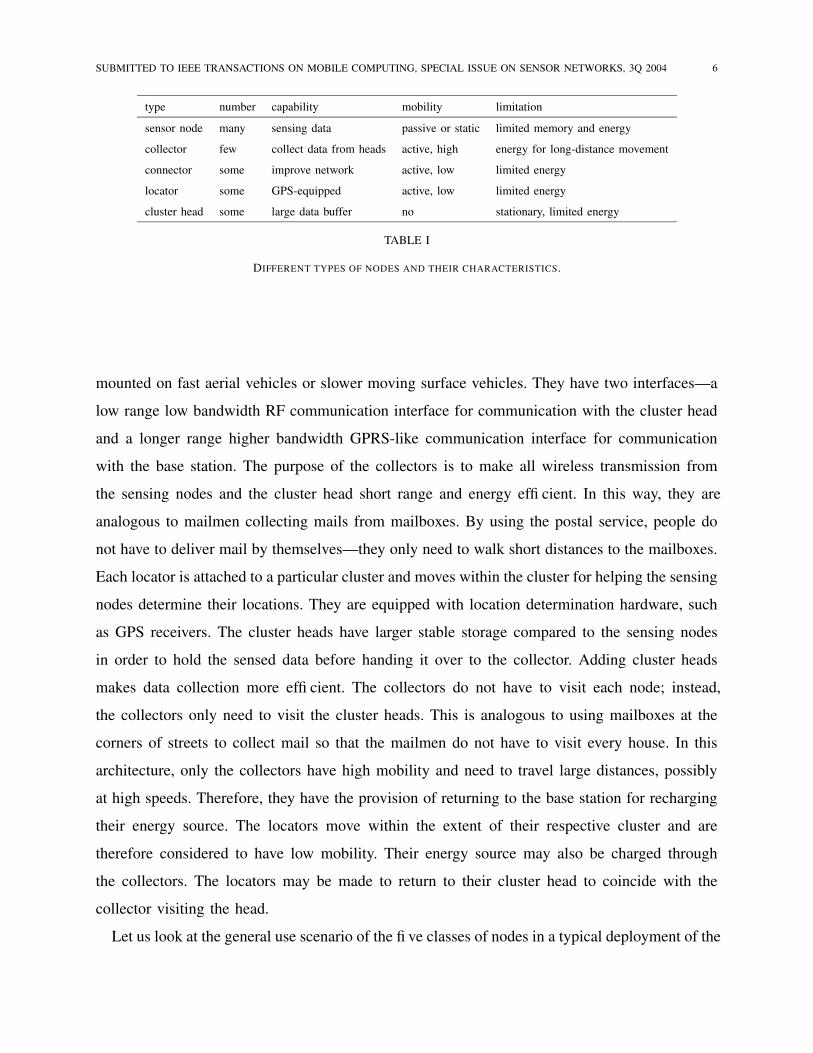
I — collectors, locators, cluster heads and connectors. The different classes of nodes and their

characteristics are summarized in Table I. A schematic of the network without the four special

classes of nodes is shown in Figure 1 and a network with the specialized nodes is shown in

Figure 2. The classes of nodes which are capable of controlled mobility have control interfaces

to which commands can be sent for the purpose of directing their motion. The collectors can be


type number capability mobility limitation

sensor node many sensing data passive or static limited memory and energy

collector few collect data from heads active, high energy for long-distance movement

connector some improve network active, low limited energy

locator some GPS-equipped active, low limited energy

cluster head some large data buffer no stationary, limited energy

TABLE I

DIFFERENT TYPES OF NODES AND THEIR CHARACTERISTICS.

mounted on fast aerial vehicles or slower moving surface vehicles. They have two interfaces—a

low range low bandwidth RF communication interface for communication with the cluster head

and a longer range higher bandwidth GPRS-like communication interface for communication

with the base station. The purpose of the collectors is to make all wireless transmission from

the sensing nodes and the cluster head short range and energy efficient. In this way, they are

analogous to mailmen collecting mails from mailboxes. By using the postal service, people do

not have to deliver mail by themselves—they only need to walk short distances to the mailboxes.

Each locator is attached to a particular cluster and moves within the cluster for helping the sensing

nodes determine their locations. They are equipped with location determination hardware, such

as GPS receivers. The cluster heads have larger stable storage compared to the sensing nodes

in order to hold the sensed data before handing it over to the collector. Adding cluster heads

makes data collection more efficient. The collectors do not have to visit each node; instead,

the collectors only need to visit the cluster heads. This is analogous to using mailboxes at the

corners of streets to collect mail so that the mailmen do not have to visit every house. In this

architecture, only the collectors have high mobility and need to travel large distances, possibly

at high speeds. Therefore, they have the provision of returning to the base station for recharging

their energy source. The locators move within the extent of their respective cluster and are

therefore considered to have low mobility. Their energy source may also be charged through

the collectors. The locators may be made to return to their cluster head to coincide with the

collector visiting the head.

Let us look at the general use scenario of the five classes of nodes in a typical deployment of the


Base Station

passively moving node

stationary node

Fig. 1. When the station is far away from all the sensor

nodes, the last-hop problem occurs.

��

��

Base Station

cluster head

mobile data collector

locator

connector

Fig. 2. Four types of special nodes are added: data collectors,

network connectors, locators, and cluster heads.

network. Initially, the nodes are deployed either through precise placement, such as manually

placed at precise pre-determined and known locations, or through pseudo-random placement,

such as light-weight nodes airdropped from a moving aerial vehicle. The network is divided into

multiple clusters based on geographical boundaries, a cluster head elected in each cluster, and

the nodes assigned to different clusters using a high energy beacon broadcast by each cluster

head. Each sensing node collects data about its immediate environment and transmits the data

to the cluster head, which is located much nearer to it than the base station. The mobile data

collectors visit the cluster heads and collect the data of the entire cluster stored there. The data

is then transmitted back by the collector to the base station. Within each cluster, the cluster

head role is rotated between the candidate set of nodes, triggered by energy getting drained or

for proximity to higher data producing nodes. The locators are equipped with GPS receivers

and move through its cluster helping the cluster heads and the passively mobile sensing nodes

determine their location. The location information for the cluster head is used by the collector

to decide its movement pattern, while the location information of the sensing nodes is used to

assign it to the closest cluster head for efficient gathering of its sensor data.


III. MOBILITY ALGORITHMS

A. Collector mobility algorithm

Let us consider initially that the nodes are static and there is a single collector which moves

through the network and collects data from the cluster heads. For the moment, we assume that

the cluster heads are fixed. We are given n cluster heads which, following the collector’s natural

traveling path (e.g. based on the geography of the sensor field), are numbered 0, . . . , n−1, such

that the collector follows the cycle of 0 → 1 → . . . → n − 1 → 0.

The cluster heads hold sensed data before the collector arrives. Since it can take a long time

— possibly hours or days — for the collector to revisit a head, it is important to determine

whether the memory in the heads is bounded. If the collector arrives later than the scheduled

time, more memory is needed in the heads. Moreover, it takes longer to transmit the data from

the heads to the collector. This requires the collector to stay longer at each cluster and further

delays the arrival of the next trip. This “positive feedback” may cause the required memory to

grow unbounded. The following analysis shows that the memory does not grow indefinitely and

hence can reach a stable schedule.

Let ri be αi/βi, for i ∈ [0, n − 1], where αi is the sensor data accumulation rate at cluster

head i and βi is the data collection rate of the mobile collector when visiting i. Let di be the

time for the collector to travel from i to i+1 (modulo n) and D be the sum of di. We have the

following linear system in terms of variables ti which represents the time taken for the collector

to collect data from each node i:

T = D +∑

i

ti (1)

ti ≥ riT (2)

ti ≥ 0 (3)

where Ineq. (2) is from the requirement of αiT ≤ βiti.

We first study the feasibility of the system defined above. Take the sum of Ineq. (2) over all

i, we have∑

i

ti ≥∑

i

riT, or T − D ≥∑

i

riT (4)


viz. T (1 −∑

i

ri) ≥ D. (5)

which is possible only if∑

i ri < 1. To show that∑

i r1 < 1 is also a sufficient condition for the

system to be feasible, we derive the solution for ti which minimizes T . (This solution minimizes

the required total buffer size for all cluster heads, since the required buffer size on each cluster

head grows linearly with T . Furthermore, minimizing T also minimizes the latency of data,

assuming that the motion of the collector takes much more time than data communication, i.e.

D À ∑

i ti. ) Suppose∑

i ri < 1 is satisfied. We let T =T̃ ≡ D/(1 − ∑

i ri) and ti = t̃i ≡ riT̃ .

T̃ and t̃i satisfy Ineqs. (2), (3) and Eq. (1) and are hence the solution which minimize T .

Next, we want to see whether the solution for ti is stable. This is important because occasion-

ally the collector’s motion schedule may be delayed unexpectedly due to transient communication

slow-down with a certain cluster head or due to changes in the travel conditions (e.g. changing

weather). It ti increases at each delay and does not return to its previous value, then the entire

motion schedule may be lengthened without an upper bound, which is an unstable situation. We

define the stability in the sense that, if the collector meets an unexpected delay at a node, the

system shown above is still feasible and ti will eventually return back to t̃i. Let ti = t̃iκ, where

κ > 1. To show that ti is still a feasible solution, we observe that T = D+κ∑

i t̃i < κT̃ . Hence,

ti = κt̃i = κriT̃ ≥ riT , satisfying Ineq. (2).

If the collector is delayed unexpectedly by an amount of time L, then each cluster head will

accumulate an additional amount, αL, of data, suppose the cluster heads have extra buffer space

to store this additional amount and thus avoid data loss. As soon the collector reaches the next

cluster head (with delay L), the cluster head empties the buffer in time κ0t̃i, for some κ0 > 1. The

collector then continues to complete the current cycle. When the next cycle begins, the collector

no longer needs to spend κt̃i at each node i. Instead, it suffices to spend ti = ri(D + κ∑

i t̃i).

The new ratio of ti over t̃i equals

κ =D + κold

∑

i t̃iD +

∑

i t̃i, (6)

which is less than κold. Hence, κ is a decreasing positive value. Take the limit on both sides

of Equation (6), we see that κ approaches 1. In other words, ti returns to t̃i. This proves the

stability of the round-robin routine.


t1 t2

(β−α)Qamount of data stored in the buffer

τ τα Q −

τ (time)

Fig. 3. The amount of data stored in the buffer rises first when the transmitter is off and then declines after it is turned on.

B. Energy considerations for buffering at cluster head

Let α be the sensing rate and β be the transmission rate. We can use a buffer to store the

sensed data during t1 in Figure 3 before transmission. The amount of stored data grows at rate α.

During t2, the transmitter is turned on. The data stored in the buffer decreases at rate β −α. At

the end of t2, the buffer is empty so the transmitter is turned off again. We assume that α < β;

otherwise, the buffer will definitely overflow. Intuitively, a larger buffer allows the transmitter

to stay off longer so more energy can be saved. However, the buffer itself also consumes power

so we have to find an appropriate buffer size which causes the most energy savings. Let pb

be the power consumed by the buffer per MB and k be the energy overhead to turn on and

off the transmitter. The buffer size Q is (α − β)t1 = βt2. We can express the value of Q asβα(α−β)(t1 + t2). During a period, the additional energy consumed by buffer insertion includes

the buffer’s energy Qpb(t1 + t2) and the overhead k for power management. The average power

if Qpb(t1+t2)+kt1+t2

= βα(α − β)pb(t1 + t2) + k

t1+t2. Our earlier study shows that the minimum power

occurs when the length of a period t1 + t2 is√

αkβpb(α−β)

and the buffer size Q is√

βkpb

(1 − βα)

[4].

C. Different mobility algorithms for collector

The collector moves among the cluster heads using one of three possible schedules—the

Round Robin schedule, the Data Rate based schedule, and the Min Movement schedule. In the

Round Robin schedule, the collector visits each cluster head to collect data in a round robin

manner. In the Data Rate based schedule, the collector visits the cluster heads preferentially.

The frequency of visiting a cluster head is proportional to the aggregate data rate from all the

nodes in the cluster. For example, take four clusters whose aggregate rate of data generation

(number of nodes times the data rate of each node) is in the ratio 1:2:3:4. Define the period


for which the collector stays at a cluster head is a slot and a consecutive number of slots over

which scheduling decisions are made as a round . With the data rate based schedule, in a round

of 10 slots, the collector will visit the cluster heads in the order 1, 2, 3, 4, 4, 3, 2, 4, 4, 3.

In the third schedule called the Min Movement schedule, the collector visits the cluster heads

in the proportion of the aggregate data rate, but also with the goal of optimizing the distance

traversed. Thus, in a round of 10 slots, the collector stays at a cluster head for multiple slots

continually, the number of slots being calculated as above depending on the aggregate data rate

at the cluster. In our simulation, this schedule gives the visit order of the cluster heads as 1, 2,

2, 3, 3, 3, 4, 4, 4, 4. The length of a slot is the time it takes for the cluster head to transfer all

the data accumulated at the cluster head till the moment the collector arrives.

D. Analysis of cluster head to collector communication

The cluster head communicates the data collected from the nodes in the cluster to the collector.

In the base case, this communication takes place once the collector reaches the cluster head.

This minimizes the transmission energy spent by the cluster head. However, as the analysis in

Section III-B shows, energy is also spent in buffering the data at the cluster head. We explore

the possibility of the cluster head transmitting some of the data to the collector as soon as

the two are within RF communication distance. In this scheme, the cluster head continues to

transmit data to the collector as the collector moves closer. The collector transmits this data to

the base station continually. This is possible since the collector uses two different communication

interfaces for communicating with the cluster head and the base station – a low bandwidth RF

interface for cluster head communication and a higher bandwidth and longer range interface for

communicating with the cluster head (such as, GPRS). The scheme has the possible advantage

of saving energy expended by the cluster head depending on when it transmits to the collector. It

has the decided advantage of reducing the data latency since the collector immediately transmits

the received data to the base station.

Let us analyze the distances over which the cluster head should transmit its data to the collector

to save the energy. We consider energy saving to be the primary concern and the latency reduction

as the consequence. We perform the analysis for one cluster without loss of generality since the

cluster specific parameters (number of nodes and rate of data generation by a node in the cluster)

are taken into account in the analysis. Let the number of nodes in the cluster be n, the rate of


data generation by each node be ρ. Let the critical distance for the data transmission be θth such

that it is energy efficient for the cluster head to transmit only after the collector is closer than

this distance. The time for the collector to traverse distance θth is tth = θth/vc, where vc is the

velocity of the collector. The energy for transmission at the cluster head has two components –

one due to the transmission circuitry which needs to be expended independent of the distance

over which the data needs to be sent, and the second component due to the power amplifier

whose energy need depends on the distance. The energy due to reception at the collector is

due to the receiver circuitry. Let the energy per bit for the two transmission components at the

cluster head be Etx elec and EPA and that for reception at the collector be Erx elec. Let the energy

expended at the power amplifier grow with the square of the transmission distance. Thus, the

energy per bit of transmission over distance d is Etx(d) = Etx elec + EPA ∗ d2. We consider an

energy efficient memory at the cluster head where the unused banks of memory may be turned

off. Thus, offloading some of the data to the collector enables the cluster head to selectively

turn off parts of its buffer thus saving its energy [5], [8], [13], [17].

Let the energy spent to keep one bit in buffer be pb. The data generated in time t by the

nodes in the cluster is nρt. This is the amount of data buffered at the cluster head. Over the time

duration tth, the total energy due to buffering is∫ ttx0 pb(nρt)dt. The amount of data transmitted

(and received) while the collector moves over a distance dθ is nρdθ/vc. The energy expended

for this data, integrated over the entire distance, is∫ θth

0 (Etx elec + EPAθ2 + Erx elec)nρ/vcdθ.

Solving the two definite integrals and equating the two sides (energy due to buffer on LHS and

energy due to RF transmission/reception on the RHS), we get the critical distance to be

pb ·θ2

th

2v= Etx elecθth + EPA

θ3th

3+ Erx elecθth (7)

For the radio used in [7], [12], Etx elec = Erx elec = 50nJ/bit and EPA = 100pJ/bit/m2.

From [5], pb = 0.012W/MB. For the collector, we use two different models – one is a fast

aerial vehicle of speed 30 m/s and the second a robot in our lab of speed 0.1 m/s [14]. The fast

collector covers the distance over which RF communication is possible for the sensor nodes in

such a short time that it is not worthwhile for the cluster head to begin transmitting. Therefore,

we do the calculation for the slow collector. Putting these values in eqn (7), we get a quadratic

equation which we solve to get the two roots for θth of 210.00 m and 14.23 m. For all practically

available sensor nodes, the RF antennas cannot communicate reliably over 210 m. We take that


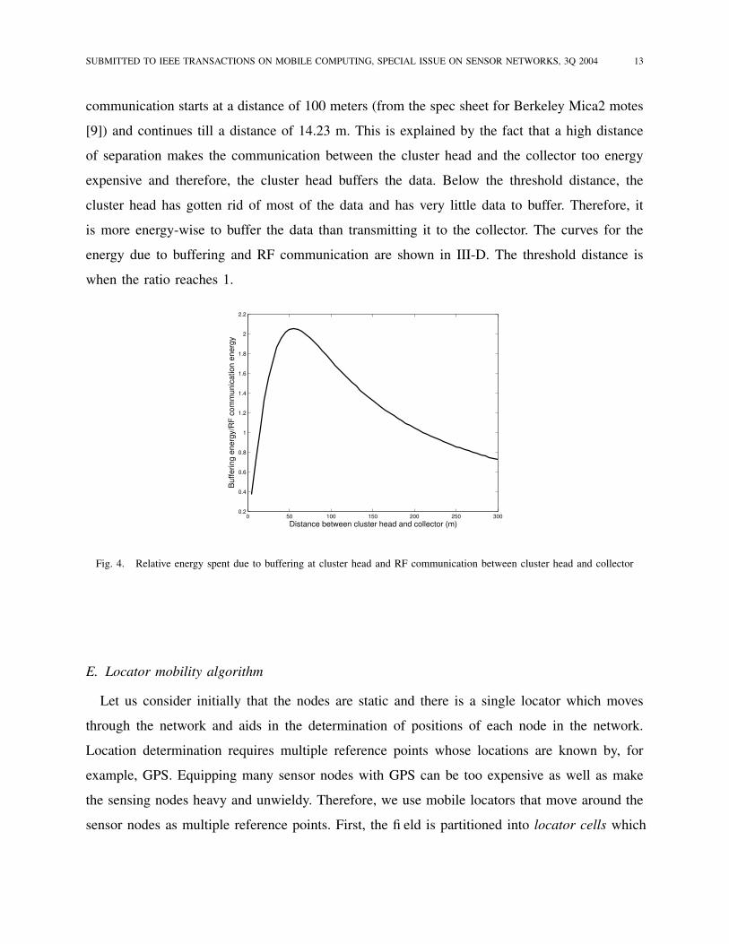
communication starts at a distance of 100 meters (from the spec sheet for Berkeley Mica2 motes

[9]) and continues till a distance of 14.23 m. This is explained by the fact that a high distance

of separation makes the communication between the cluster head and the collector too energy

expensive and therefore, the cluster head buffers the data. Below the threshold distance, the

cluster head has gotten rid of most of the data and has very little data to buffer. Therefore, it

is more energy-wise to buffer the data than transmitting it to the collector. The curves for the

energy due to buffering and RF communication are shown in III-D. The threshold distance is

when the ratio reaches 1.

0 50 100 150 200 250 3000.2

0.4

0.6

0.8

1

1.2

1.4

1.6

1.8

2

2.2

Distance between cluster head and collector (m)

Buf

ferin

g en

ergy

/RF

com

mun

icat

ion

ener

gy

Fig. 4. Relative energy spent due to buffering at cluster head and RF communication between cluster head and collector

E. Locator mobility algorithm

Let us consider initially that the nodes are static and there is a single locator which moves

through the network and aids in the determination of positions of each node in the network.

Location determination requires multiple reference points whose locations are known by, for

example, GPS. Equipping many sensor nodes with GPS can be too expensive as well as make

the sensing nodes heavy and unwieldy. Therefore, we use mobile locators that move around the

sensor nodes as multiple reference points. First, the field is partitioned into locator cells which


are disjoint rectangular regions that satisfy a necessary condition (condition 1) and an optional

condition (condition 2).

1) The maximum separation of two nodes in the cell is less than the transmission range of

the nodes (Necessary).

2) The number of nodes in a cell is greater than a threshold, denoted by ητ (Optional).

A cell which satisfies both conditions is called a complete cell, and one which satisfies only the

necessary condition is called an incomplete cell. Note that a cell is different from a cluster. A

cell is purely for the purpose of determining locator movement, while a cluster is an aggregate

of nodes which have a cluster head that collects and possibly processes data from all the cluster

nodes. A cluster comprises multiple cells. A cell is a square region of dimension < (transmission

range)/2√

2.

The given parameters for the sensor network under consideration are the following.

• Allowable error in location estimation (ετ ). Each node should determine its location with

less than ετ error on an average. The error arises due to errors in the model correlating

physical measurement with distance between one-hop neighbors. This is a requirement

imposed on the localization system. The error is given in terms of distance units that the

calculated location can differ from the actual location.

• Velocity of locator (vl). This is the maximum speed with which the locator can navigate

within the cluster.

• Epoch (ζS). This is the average duration between successive movements of a passively

mobile node.

The locators are mobile and each locator can act as multiple reference points for location

estimation by communicating with a sensing node at different time points. The locators are looked

upon as mobile entities that roam the sensor field, periodically broadcasting beacon messages

with their own locations. An intermediate node when it receives a beacon message, it forwards

it after incrementing the hop count. Thus, receiving a beacon message, a passively mobile node

can estimate the number of hops it is away from the locator. The sensing nodes collect the

beacon messages and after an appropriate number of beacon messages perform triangulation to

determine their locations. A sensing node knows the number of beacon messages required in

order for the location estimation error to be below ετ . The error in the estimation (ε) is a function


of the number of beacon messages (ηb) and the distance between the node and the locator for

each reference point (δl,n). The distance can be approximated by the product of the number of

hops separating the locator and the node (hl,n), and the transmission range of each node (rT ).

The locator has the same kind of RF communication device as the sensing nodes and hence, its

transmission range is considered identical to that of the sensing nodes.

ε = F (δl,n, ηb) = F (hl,n · rT , ηb) (8)

F. Determination of Localization Error

We wish to determine the number of beacon messages that should be collected by a sensing

node to guarantee a desired accuracy in its location estimate. The guarantee will however be

probabilistic, i.e., the guarantee will be stated in terms of a probability that the error in location

estimate will be bounded by a desired value. We will start with some background for location

estimation. We will present this discussion in terms of a sensing node being surrounded by

multiple neighbors each of which knows its own location. The neighbors send beacon messages

to the sensing node using which it determines its location. Our environment where there is a

single locator that moves and sends beacon messages from multiple positions is easily mapped

to this model. The minimum number of neighbors required for location estimation in an n

dimensional plane is (n + 1). Thus, in our special case of a 2-dimensional plane, 3 neighbors

are required, under perfect conditions, namely, where individual distance measurements from a

neighbor are completely accurate. Localization with respect to three neighbors gives the following

set of equations.

(x1 − ux)2 + (y1 − uy)

2 = r21

(x2 − ux)2 + (y2 − uy)

2 = r22

(x3 − ux)2 + (y3 − uy)

2 = r23 (9)

In this set of equations, (ux, uy) is the position of the sensing node that we intend to locate and

(xi, yi) is the location of the ith neighbor. Solving equation 9 we get ux to be of the following

form.


ux = k1r21 + k2r

22 + k3r

23 + k4 (10)

where ki ∈ R. Similarly, uy can be expressed in a form like equation10. One simple relation

for measuring error in ux and uy is to differentiate both sides of the equation to get ∆ux =

2k1r1∆r1+2k2r2∆r2+2k3r3∆r3. However, this is dependent on topology and no obvious bounds

exist for the error. We choose to work with variances as a measure of the error in estimation.

The range measurements are error prone, and this leads to the error in location estimation of the

sensing node. If we assume that the errors in range measurements are uncorrelated, then from

equation10, we get the variance of the estimated location in the following form.

V ar(ux) = k21V ar(r2

1) + k22V ar(r2

2) + k23V ar(r2

3) (11)

For the purpose of estimating the error, we consider the neighbors to be divided into groups of

3. Triangulation is performed as above for each such group. Each triangulation gives a sample

value for ux and uy and the location of the sensing node is finally determined by taking an

average of all these ux and uy values. For simplicity we consider the number of neighbors to be

an integral multiple of 3. Thus, the number of sample values of ux and uy is p = N/3 where

N is the number of neighbors. The expected value of the calculated location (i.e., the sample

mean) is the same as the expected value of the population mean and thus the technique gives

an unbiased estimate of the location. The variance of the estimated location is given by.

V ar(uxp) = V ar(ux)/p (12)

Note that V ar(uxp) is the ensemble variation in space over neighbors that form an ensemble,

while the variance V ar(ux) computed in equation11 is the time variance. Consider that the

measurements of the range vector [r1, r2, r3] represent a stochastic process in time. So the

averaging for determination of ux and uy is done over time and therefore the variance in

equation11 is a time variance. On the other hand, in averaging over p = N/3 samples, we

are averaging over the neighbors of the sensing node and this is an ensemble average. The

corresponding variance is also the ensemble variance. If we assume ergodicity of the mean and

the variance, then the time average and variance can be replaced by the ensemble average and

variance that we need for our subsequent analysis.


Chebyshev’s inequality gives that for a random variable X with a distribution having finite

mean µ and finite variance σ2, P (|X − µ| ≥ t) ≤ σ2/t2, t ≥ 0. Applying this to the random

variable uxp we get Probability (Error in location estimate (for the x-axis) ≥ Error bound in

distance units) as follows.

P (|uxp − E(uxp)| ≥ ε) ≤ 1/ε2 · V ar(uxp)

P (|uxp − E(ux)| ≥ ε) ≤ 1/(pε2) · V ar(ux) (13)

Equation13 gives a bound on the probability of error in estimated location exceeding a desired

threshold in terms of the number of neighbors. Given a desired accuracy, we can make the

probability of error exceeding the desired accuracy to be as small as we like by increasing p,

i.e., by extension, increasing the number of neighbors. Next, we have to determine the variance

in ux to complete the analysis. In equation11, if we take that the errors in the three range

measurements r1, r2, r3 are equal, then the variance in ux can be written as.

V ar(ux) = (k21 + k2

2 + k23)V ar(r2) (14)

In general, the coefficients k1, k2, k3 are dependent on topology, i.e., the relative placements

of the neighbors with respect to the sensing node. The upper bound for the sum is infinity

(when the three neighbors are collinear) and the lower bound is achieved when the triangles

formed by the neighbors with the sensing node are equilateral. We perform an analysis on the

topology shown in Figure 5. For values of angle θ subtended by the neighbors at the anchor

node ( 6 CAD = 6 BAC = θ) between 536

π(25◦) and 13π(60◦), it can be shown that k2

1 + k22 + k2

3

lies close to 0.2/R where R is the distance between the neighbor and the sensing node. By our

algorithm, the locator sends beacon messages when it is either in the cell or in the adjacent cell

to the sensing node and therefore R ≤ rT , where rT is the transmission range.

Next, we compute V ar(r2). Consider the error in range measurements and let the upper bound

on the relative error be e. This means that if the actual distance between a neighbor and the

sensing node is d, the measurement lies between d± e · d. Assume that the range measurements

follow a Gaussian distribution. Therefore, almost all the points (99.74% to be exact) lie within

µ±3σ. Equating, σ = ed/3. The upper bound for this is erT /3. Thus, V ar(r) ≤ (erT /3)2. Then,

V ar(r2) = E(r4)− (E(r2))2. The higher order expectations can be calculated using the moment


B

DC

A

��

��

��

SensingNode Node

Anchor��

Fig. 5. Topology of sensing node and 3 neighboring anchor nodes. Triangulation is done by the sensing node using distance

measurements from the three anchor nodes.

generating function of a Gaussian distribution with mean µ and variance σ2 M(t) = eµt+σ2t2/2.

E(r2) and E(r4) can be derived by differentiating M(t) respectively twice and four times and

evaluated at t=0. Simplifying, we get from equation14 the Probability (Error in location estimate

(for the x-axis) ≥ Error bound in distance units) as

P (|uxp − E(uxp)| ≥ ε) ≤ 1/(pε2) · 0.2e2R3(2.47X10−2e2 + 4.44X10−1) (15)

For our environment, we pick p = 24 to restrict the error in location estimation in each

dimension to 10 meters. Note that the above bound can be made much tighter for smaller

distances between the neighboring node and the sensing node and for particular topologies. This

value of p corresponds to a total of 72 beacon messages by the locator for the nodes in one cell.

This means that the number of beacon messages sent out by the locator from each cell (the cell

itself and its 8 neighboring cells) is 8.

Once the required number of beacon messages are received by a sensing node, it determines

its location. The sensing node then informs the locator of its location. The locator verifies this

location using the received signal strength from the node. Then, it assigns the node to the

appropriate cluster. In a majority of cases, the node will be assigned to the cluster to which

the locator is coupled. Only if the node has moved far away will it be reassigned to a possibly

closer cluster head.

Again considering cell i, the locator sends a beacon message while located in cell i. The cells


in Ci1 are ordered according to the metric (Number of nodes in the cell - Distance of the cell

from the current position). The complete and incomplete cells are ordered separately with all the

complete cells being ordered above the incomplete cells. The locator picks the next cell to visit

in order from the ordered list. Next, the cells in Ci1 are ordered, and so on. The movement is

stopped when any node in the cell indicates that it has the requisite number of beacon messages.

A constraint for the movement of the locator is that all the ητ beacon messages must be

received by a node before it moves. Let the distance between two cells ci and cj be given by

δi,j . The locator has sent ηc beacon messages for cell i and in time tc. The locator is currently

in cell m and the next cell in the ordered list is cell n. The condition that the locator seeks to

enforce is (ητ − ηC) · δi,j

vl< (ζS − tc). If the condition is violated for cell n, the locator moves to

another position within the same cell m and sends another beacon message. This probabilistically

assures that all beacon messages are received in the time in which it is useful, i.e. between two

movements of a node.

IV. EXPERIMENTS AND RESULTS

We perform simulations using the NS-2 simulator [22]. The simulation environment is set up

as follows. There are four clusters that are separated over a distance such that any two nodes

from different clusters are not able to communicate between each other. Each cluster has a

cluster head that collects data from its own cluster. Since the cluster head does not have the

capability to send the collected data to the base station, there is a mobile data collector which

moves to and collects data from each cluster head. The mobile collector then sends the data to

the base station for analysis. The large inter-cluster distance and the separation from the base

station underline the need for a mobile collector as opposed to multiple relay nodes between the

cluster heads and the base station.

In each simulation, a cluster sends data, at a constant rate, to its own cluster head. The cluster

head stores the data in its buffer until the data collector arrives (either physically, or within

the energy-efficient communicable distance) and collects the data via wireless communication.

The data collector follows a predetermined movement schedule to visit each cluster head. The

collector periodically goes back to the base station if it does not have enough energy to serve

another cluster head. Each cluster is characterized by the position of the cluster head, the number

of nodes in the cluster, and the aggregate data rate of the cluster. In our simulation, we consider


Cluster Parameter #1 #2 #3 #4

Cluster head coordinate (m) (1,800) (1,1) (800,1) (800,800)

(Base station is at (400,1500))

Data rate per cluster node 2 bps 4 bps 6 bps 8 bps

Number of nodes in cluster 500 500 500 500

TABLE II

CHARACTERISTICS OF CLUSTERS

heterogeneous clusters. For the simulation, the cluster head is considered non-rotating. Since the

geographical spread of the cluster is much smaller than the inter-cluster distance, we believe this

will not have much effect on the results. The four clusters with the positions of the cluster heads

and the base station is shown in Figure IV. The spread of only cluster number 2 is shown. The

characteristic of the four clusters is summarized in Table II.

40 m

(400,1500)Base Station

��

��

(1,1)CH2

(800,1)CH3

(800,800)CH4

(1,800)CH1

Fig. 6. Topology of the four clusters and the base station used for simulation

The energy model used for the cluster head is the same as for the radio used in [7], [12]. The

energy has two components—one due to the transmit-receive circuitry and the other due to the

power amplifier. The latter component depends on the distance over which the data is transmitted.

The amount of energy to send n bits of data over a distance d is given by n(ETxRx+EPAd2). The

bandwidth for the cluster head to collector communication follows the value for the Berkeley


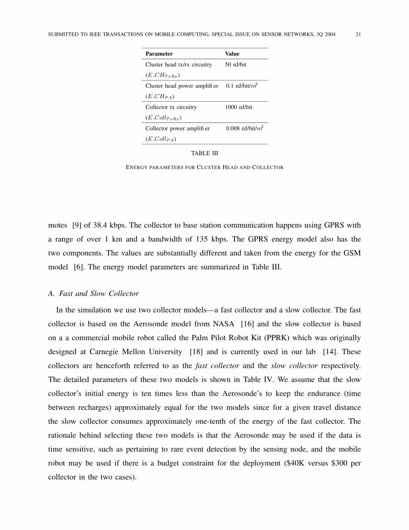
Parameter Value

Cluster head tx/rx circuitry 50 nJ/bit

(E CHTxRx)

Cluster head power amplifier 0.1 nJ/bit/m2

(E CHPA)

Collector tx circuitry 1000 nJ/bit

(E CollTxRx)

Collector power amplifier 0.008 nJ/bit/m2

(E CollPA)

TABLE III

ENERGY PARAMETERS FOR CLUSTER HEAD AND COLLECTOR

motes [9] of 38.4 kbps. The collector to base station communication happens using GPRS with

a range of over 1 km and a bandwidth of 135 kbps. The GPRS energy model also has the

two components. The values are substantially different and taken from the energy for the GSM

model [6]. The energy model parameters are summarized in Table III.

A. Fast and Slow Collector

In the simulation we use two collector models—a fast collector and a slow collector. The fast

collector is based on the Aerosonde model from NASA [16] and the slow collector is based

on a a commercial mobile robot called the Palm Pilot Robot Kit (PPRK) which was originally

designed at Carnegie Mellon University [18] and is currently used in our lab [14]. These

collectors are henceforth referred to as the fast collector and the slow collector respectively.

The detailed parameters of these two models is shown in Table IV. We assume that the slow

collector’s initial energy is ten times less than the Aerosonde’s to keep the endurance (time

between recharges) approximately equal for the two models since for a given travel distance

the slow collector consumes approximately one-tenth of the energy of the fast collector. The

rationale behind selecting these two models is that the Aerosonde may be used if the data is

time sensitive, such as pertaining to rare event detection by the sensing node, and the mobile

robot may be used if there is a budget constraint for the deployment ($40K versus $300 per

collector in the two cases).


Parameter Fast Collector Slow Collector

(Aerosonde) (Mobile Robot)

Speed 30 m/sec 0.1 m/sec

Energy consumed 10 Joule/sec 0.97 Joule/sec

' 0.33 Joule/m ' 9.7 Joule/m

Initial energy 1.44 MJoule 144 KJoule

TABLE IV

CHARACTERISTICS OF FAST AND SLOW COLLECTOR USED IN THE SIMULATION

For the simulation, in the slow collector case, the cluster head transfers data to the collector

through wireless RF communication for the optimal distance range as calculated in Section III-D.

For the fast collector, however, this distance is traversed so fast that we make the simplification

that cluster head only transfers data to the collector, once the collector arrives at the cluster head.

B. Collector Movement Schedule

Recollect that the collector moves among the cluster heads using one of three possible

schedules—the Round Robin schedule, the Data Rate based schedule, and the Min Movement

schedule. In a round of 10 slots, the collector will visit the cluster heads in the order 1, 2, 3, 4,

1, 2, 3, 4, 1, 2 in the Round Robin schedule; 1, 2, 3, 4, 4, 3, 2, 4, 4, 3 in the Data Rate based

schedule; and 1, 2, 2, 3, 3, 3, 4, 4, 4, 4 in the Min Movement schedule. The length of a slot

is the time it takes for the cluster head to transfer all the data accumulated at the cluster head

till the moment the collector arrives (either physically arrives at the cluster head or data transfer

through RF communication starts).

We also consider the possibility of variation in the physical conditions of the environment

affecting the speed of the collector. The collector may face an obstacle in its path and may

have to deviate from part of its pre-calculated route. Also, the physical conditions, such as wind

speed, may change thereby affecting the collector speed. In order to take such variations into

account, the speed of the collector is varied according to a normal distribution, such that the

speed can vary by ± 40% of the average speed. This means that the 3σ limit of the Normal

distribution is taken as ± 40% of the average.


C. Output Parameters

We collect the following output parameters from the simulation of the collector.

• Buffer size at the cluster head

• Data latency for data generated by the sensing nodes

• Time between recharges of the collector

The output parameters are calculated based on 50 rounds of collector movement after the

initial transient period ends. The initial transient period is characterized by continuous growth in

the buffer occupancy at the cluster heads. Each round is defined as 10 slots of movement. The

buffer size in bytes is the buffer required at the cluster head for the data generated by the sensing

nodes before it is handed over to the collector. Due to the variation in the speed of the collector,

the buffer size also varies between rounds. We take the maximum buffer size over all the rounds

after throwing out the outliers that lie beyond the 2σ range. The maximum buffer size is the

relevant metric since the cluster head will have to provision for a buffer of that size to prevent

data loss due to overflow. Throwing out the outliers is needed to eliminate the statistical noise

and to draw useful conclusions from the results. The data latency is measured as the average

of the time gap between the data generated by the sensing node and the data reaching the base

station. We approximate the time the data is generated by the sensing node by the time the data

reaches the cluster head. The collector returns to the base station when it estimates its energy

will run out before it can reach the next cluster head and collect all its data. The third output

parameter is the average time between successive visits of the collector to the base station for

recharging.

D. Experiment Set 1: Fast Collector

In the fast collector, we observe the collector has a very high endurance and rarely returns to

the base station for recharge. Therefore, the output parameter of average time between recharges

is omitted for this set of experiments. The results are presented in Table V.

In the Data Rate based schedule, the buffer size that cluster head 1, 2, and 3 need is almost

similar, but not for cluster head 4. The increasing amount of buffer size in the Data-Rate based

scenario for cluster heads 1, 2, and 4 compared to the Round Robin schedule is because the

maximum the number of cluster head(s) that a collector needs to visit before successive visits to


Round Robin Data Rate based Min Movement

CH1 22.43 50.88 44.30

Buffer Size CH2 44.93 54.62 80.00

(KBytes) CH3 66.53 63.30 107.22

CH4 87.92 111.56 124.37

CH1 75.04 181.29 153.79

Data Latency CH2 75.11 93.18 76.99

(sec) CH3 75.05 62.19 51.36

CH4 74.93 46.61 38.55

TABLE V

RESULTS FOR FAST COLLECTOR WITH THREE DIFFERENT MOVEMENT SCHEDULES

cluster head 1, 2, and 4 is 9, 4, and 4 respectively. This is higher than the successive visits in the

Round Robin schedule (3 for all the cluster heads). On the other hand, the gap between successive

visits for cluster head 3 is 2 which leads to the decreasing amount of buffer needed. The same

reasoning happens in the Min Movement scenario since the successive visits to each cluster head

are spread farther apart than the Round-Robin and so is the amount of buffer needed to hold

the data. The decrease of average latency in Data Rate based and Min Movement compared to

Round Robin is because both these schedules consider the data rate of each cluster—the higher

the data rate, the more often the cluster is visited by the collector. The latency is averaged over

the entire data and is therefore improved.

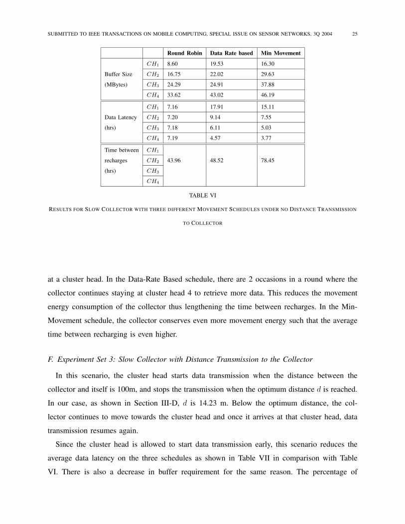
E. Experiment Set 2: Slow Collector without Distance Transmission to the Collector

In this set of experiments, we consider the slow collector that waits for the collector to arrive

at its location before transferring data to the collector. The buffer size, latency and time between

recharges is shown in Table VI.

In this result, the buffer size needed by each cluster is higher compared to the fast collector

case in Table V. The reasoning is that the collector speed is much slower such that each cluster

produces more data between successive visits which also increases the data collection time of the

collector. The frequency of recharge in Round-Robin schedule is higher compared to the other

two schedules since the collector has to move each time it has finished collecting all the data



CH1 8.60 19.53 16.30

Buffer Size CH2 16.75 22.02 29.63

(MBytes) CH3 24.29 24.91 37.88

CH4 33.62 43.02 46.19

CH1 7.16 17.91 15.11

Data Latency CH2 7.20 9.14 7.55

(hrs) CH3 7.18 6.11 5.03

CH4 7.19 4.57 3.77

Time between CH1

recharges CH2 43.96 48.52 78.45

(hrs) CH3

CH4

TABLE VI

RESULTS FOR SLOW COLLECTOR WITH THREE DIFFERENT MOVEMENT SCHEDULES UNDER NO DISTANCE TRANSMISSION

TO COLLECTOR

at a cluster head. In the Data-Rate Based schedule, there are 2 occasions in a round where the

collector continues staying at cluster head 4 to retrieve more data. This reduces the movement

energy consumption of the collector thus lengthening the time between recharges. In the Min-

Movement schedule, the collector conserves even more movement energy such that the average

time between recharging is even higher.

F. Experiment Set 3: Slow Collector with Distance Transmission to the Collector

In this scenario, the cluster head starts data transmission when the distance between the

collector and itself is 100m, and stops the transmission when the optimum distance d is reached.

In our case, as shown in Section III-D, d is 14.23 m. Below the optimum distance, the col-

lector continues to move towards the cluster head and once it arrives at that cluster head, data

transmission resumes again.

Since the cluster head is allowed to start data transmission early, this scenario reduces the

average data latency on the three schedules as shown in Table VII in comparison with Table

VI. There is also a decrease in buffer requirement for the same reason. The percentage of



CH1 7.60 17.33 16.28

Buffer Size CH2 15.21 19.46 28.43

(MBytes) CH3 21.94 22.27 37.08

CH4 29.16 39.33 45.73

CH1 6.37 16.08 14.36

Data Latency CH2 6.37 8.25 7.17

(hrs) CH3 6.35 5.49 4.78

CH4 6.34 4.12 3.59

Time between CH1

recharges CH2 45.83 49.21 79.83

(hrs) CH3

CH4

TABLE VII

RESULTS FOR SLOW COLLECTOR WITH THREE DIFFERENT MOVEMENT SCHEDULES UNDER DISTANCE TRANSMISSION TO

COLLECTOR

improvement is shown in the Table VIII.

In Table VIII, the Min-Movement schedule has less improvement due to distance transmission

because the collector often stays at a particular cluster head for consecutive slots. The fraction

of time over which distance transmission happens in the Min-Movement schedule in relation to

the time the collector spends at a cluster head is smaller than in the other movement schedules.

Hence, the relative improvement due to the distance transmission is smaller.

The Round Robin schedule helps the recharge interval more than the other schedules. This

can be explained by the observation that for cluster 1, the lowest data rate cluster, the collector

does not always have to physically arrive at the cluster head. In some cases, all the data is

communicated to the collector through distance transmission. In that case, the collector directly

goes to the next cluster in its schedule (cluster 2). The distance traversed to go to cluster head

2 is less in this case compared to reaching cluster head 1 and then proceeding to cluster head 2.

This is thus energy efficient and lengthens the time period between recharges of the collector.



CH1 11.64% 11.24% 0.15%

Buffer Size CH2 9.22% 11.65% 4.04%

CH3 9.70% 10.61% 2.10%

CH4 13.28% 8.56% 1.00%

CH1 11.01% 10.21% 5.02%

Data Latency CH2 11.57% 9.77% 5.02%

CH3 11.56% 10.15% 5.06%

CH4 11.84% 9.77% 4.94%

Time between CH1

recharges CH2 4.25% 1.42% 1.76%

CH3

CH4

TABLE VIII

IMPROVEMENT FOR SLOW COLLECTOR WITH DISTANCE TRANSMISSION TO COLLECTOR

G. Experiment Set 4: Locator

For the locator, we use a commercial mobile robot (PPRK) ( [14], [18]) (same as the one used

for the slow collector), equipped with the Global Positioning System (GPS) carrying a regular

sensor node with capability for short range RF communication. The locator moves in the cluster

with 500 sensing nodes randomly distributed in the cluster spread. All the sensing nodes need

to determine their own positions with the help of the locator. The cluster is divided into cells

of size 10m x 10m and the size of the cluster is taken to be a square region of dimension 80m

x 80m which inscribes the circular cluster region. The locator is capable of broadcasting its

own position to the neighboring sensing nodes within a range of 30m. Thus, a locator in a cell

can reach all the nodes in its own cell and in the 8 adjoining square cells (diagonal length =

2 ·√2 ·10 < 30 m. The locator is unaware of the locations of individual sensing nodes. However,

it knows the boundary of the cluster.

With this information, the locator moves from one cell to another in an ”S” pattern as shown

in Figure 7. The number of sensing nodes in each cell is shown by the number in the lower

right corner in each cell. During the course of its movement, the locator broadcasts 8 beacon


messages in 8 different random positions within each cell. Each beacon message contains the

position information of the locator. Since the size of each beacon message is 36 bytes (default

packet size in TinyOS [9]) and the locator’s bandwidth is 38,400 bps, the locator stays in each

position for broadcasting a beacon for 7.5 ms. In order to simulate a real world situation, we

vary the locator’s speed by using a normal distribution, where on an average the locator moves

10cm/s with a variance of ±40% (same as for the land robot for the slow collector). Each sensing

node needs to receive 72 beacon messages in order to determine its position with error in each

dimension of less than 10 m.

Fig. 7. Movement of the locator within a cluster Fig. 8. Rate of dissemination of location information among

sensing nodes in a cluster

We are interested in three output parameters for the locator. The first is the rate at which

location information is disseminated in the cluster. This is shown in Figure 8. The x-axis is the

time elapsed since the locator started its movement in the cluster. The y-axis is the fraction of

the nodes in the cluster that have determined their location. The second parameter of interest

is the total time measured from the time the locator starts moving in the cluster such that all

the nodes in the cluster know their position. For our simulation, this is 109,359.65 seconds ('30.38 hours). This can be read off from the curve in Figure 8 by considering the time for the

y-axis value to be 1.0. This time can be looked upon as the worst case initial latency when

none of the nodes know their location to start with. In the steady state, only a few of the nodes

will move and an incremental location determination will be needed. For this reason, we are

interested in the third parameter, which is the time for a node to determine its location once the


locator arrives in its vicinity. This is given by the time to move among the cell in which the

node is located and the 8 adjoining cells and broadcast 8 beacon messages from each cell. For

our simulation, this time is 2882.39 seconds (= 0.8 hours). This is also the time for which the

node will have to be stationary for the location determination to be useful. This number appears

high and is due to the slow speed of the locator (0.1 m/s) compared to the transmission range

(30 m). In a network deployment, this will be determined by the estimated pause time in the

movement of a node and a locator of an appropriate speed will be chosen.

V. CONCLUSION

In this paper, we have proposed an architecture for energy efficient data gathering in large

scale sensor networks. Some sensing nodes in the network may be passively mobile which makes

the problem more challenging. In the network model under consideration, the sensor field has a

large geographical spread and many of the sensing nodes are far away from the base station. We

introduce some special classes of nodes some of which have the capability of controlled mobility,

i.e., mobility of the form that can be directed by sending control signals. The data collectors

have the capacity for moving over long distances, possibly at high speeds for collecting data

from the cluster heads and communicating the data back to the base station. The cluster heads

aggregate the data from the nodes in the cluster and temporarily store them prior to transmission

to the collector. In order to enable efficient data gathering from the passively mobile sensing

nodes, they need to be associated with the closest cluster head and therefore, need to know their

locations. This is enabled by GPS-equipped mobile locators which move through the cluster and

broadcast beacon messages with location information that helps the sensing nodes determine

their position.

In this paper, we propose algorithms for motion of the data collectors and the locators. We

also propose an extension to the traditional triangulation approach for location determination

using mobile locators. The algorithms are analyzed mathematically and simulated to bring out

their important characteristics, such as energy consumption, data latency and cluster head buffer

requirement (collector algorithm), and convergence time (locator algorithm).

For future work, we plan to consider the movement patterns of the passively mobile sensing

nodes in a cluster. We wish to investigate what proactive information broadcast by these passively

mobile nodes can benefit the algorithms by making them more informed about the sensor field,


such as the density of nodes in a region. We are also investigating the effect of failures of

collectors or cluster heads on the data collection. A set of cluster heads can concurrently serve

the role. Also cooperation between multiple cluster heads to overcome temporary periods of

high data rate is possible. There may be multiple collectors in the network which may work

cooperatively in servicing the different cluster heads. Alternately, there may be a set of collectors

for emergency data gathering corresponding to rare events being detected by a sensing node.

The mobility algorithms needs to take these classes of collector nodes into account.

REFERENCES

[1] I. F. Akyildiz, W. Su, Y. Sankarasubramaniam, and E. Cayirci. A Survey on Sensor Networks. IEEE Communications

Magazine, 40(8):102–114, August 2002.

[2] S. Basagni, I. Chlamtac, V. R. Syrotiuk, and B. A. Woodward. A Distance Routing Effect Algorithm for Mobility (DREAM).

In International Conference on Mobile Computing and Networking, pages 76–84, 1998.

[3] S. Cabuk, N. Malhotra, L. Lin, S. Bagchi, and N. Shroff. Analysis and evaluation of topological and application

characteristics of unreliable mobile wireless ad-hoc network. In Proceedings of the 10th Pacific Rim Dependable Computing

Conference, March, 2004 (PRDC 04), March 2004.

[4] L. Cai and Y.-H. Lu. Dynamic Power Management Using Data Buffers. In Design Automation and Test in Europe, pages

526–531, 2004.

[5] L. Cai and Y.-H. Lu. Dynamic power management using data buffers. In Design Automation and Test in Europe, 2004.

[6] D. Estrin, M. Srivastava, and A. Sayeed. Wireless sensor networks. MOBICOM 2002 Tutorial T5.

[7] W. Heinzelman, A. Chandrakasan, and H. Balakrishnan. Energy-efficient communication protocol for wireless microsensor

networks. In 33rd International Conference on System Sciences (HICSS ’00), January 2000.

[8] C. Im, H. Kim, and S. Ha. Dynamic Voltage Scheduling Technique for Low-power Multimedia Applications Using Buffers.

In International Symposium on Low Power Electronics and Design, pages 34–39, 2001.

[9] C. Inc. Mpr/mib mote hardware users manual. URL: http://www.xbow.com/Support/Support pdf files/MPR-

MIB Series User Manual 7430002105 A.pdf.

[10] Y. Ko and N. Vaidya. Location-aided routing (lar) in mobile ad hoc networks. Wireless Networks, pages 307–321, July

2000.

[11] A. LaMarca, D. Koizumi, M. Lease, S. Sigurdsson, G. Barriello, W. Brunette, K. Sikorski, and D. Fox. Making Sensor

Networks Practical With Robots. Technical report, Intel Research, IRS-TR-02-004, 2002.

[12] S. Lindsey, C. Raghavendra, and K. M. Sivalingam. Data gathering algorithms in sensor networks using energy metrics.

IEEE Transactions on Parallel and Distributed Systems, 13:924–935, 2002.

[13] Y.-H. Lu, L. Benini, and G. D. Micheli. Dynamic Frequency Scaling With Buffer Insertion for Mixed Workloads. IEEE

Transactions on Computer-Aided Design of Integrated Circuits and Systems, 21(11):1284–1305, November 2002.

[14] Y. Mei, Y.-H. Lu, C. G. Lee, and Y. C. Hu. Energy-efficient motion planning for mobile robots. In International Conference

on Robotics and Automation 2004 (ICRA ’04), 2004.

[15] D. P. Miller, T. S. Hunt, and M. J. Roman. Experiments and Analysis of The Role of Solar Power in Limiting Mars Rover

Range. In IEEE/RSJ International Conference on Intelligent Robots and Systems, pages 317–322, 2003.


[16] NASA. Aerosonde unmanned aerial vehicle, manufactured by aerosonde robotic aircraft limited. URL:

http://uav.wff.nasa.gov/UAVDetail.cfm?RecordID=Aerosonde.

[17] Q. Qiu, Q. Wu, and M. Pedram. Dynamic Power Management in A Mobile Multimedia System With Guaranteed Quality-

of-service. In Design Automation Conference, pages 834–839, 2001.

[18] G. Reshko, M. Mason, and I. Nourbakhsh. Rapid prototyping of small robots. Technical Report CMU-RI-TR-02-11,

Robotics Institute, Carnegie Mellon University, Pittsburgh, PA, March 2002.

[19] P. E. Rybski, N. P. Papanikolopoulos, S. A. Stoeter, D. G. Krantz, K. B. Yesin, M. Gini, R. Voyles, D. F. Hougen, B. Nelson,

and M. D. Erickson. Enlisting Rangers and Scouts for Reconnaissance and Surveillance. IEEE Robotics and Automation

Magazine, 7(4):14–24, December 2000.

[20] G. T. Sibley, M. H. Rahimi, and G. S. Sukhatme. Robomote: A Tiny Mobile Robot Platform for Large-scale Ad-hoc

Sensor Networks. In International Conference on Robotics and Automation, pages 1143–1148, 2002.

[21] A. Tsirigos and Z. J. Haas. Multipath routing in the presence of frequent topological changes. IEEE Communications

Magazine, 39:132–138, November 2001.

[22] USC/ISI. The network simulator — ns-2. URL: http://www.isi.edu/nsnam/ns/.

CERIAS Tech Report 2005-92 CONTROLLED … Tech Report 2005-92 CONTROLLED MOBILITY FOR EFFICIENT DATA...

Documents

Transcript of CERIAS Tech Report 2005-92 CONTROLLED … Tech Report 2005-92 CONTROLLED MOBILITY FOR EFFICIENT DATA...