CERES EBAF Ed2.8 Data Quality Summary (March 19, 2014)€¦ · Data Quality Summary (March 19,...

CERES_EBAF_Ed2.8 3/19/2014 Data Quality Summary (3/19/2014)

CERES_EBAF_Ed2.8

Data Quality Summary (March 19, 2014)

Investigation: CERES Data Product: EBAF Data Set: Terra (Instruments: CERES-FM1 or CERES-FM2) Aqua (Instruments: CERES-FM3 or CERES-FM4) Data Set Version: Edition2.8 Subsetting Tool Availability: http://ceres.larc.nasa.gov/order_data.php The purpose of this document is to inform users of the accuracy of this data product as determined by the CERES Science Team. The document summarizes key validation results, provides cautions where users might easily misinterpret the data, provides links to further information about the data product, algorithms, and accuracy, and gives information about planned data improvements. This document provides a high-level quality assessment of the CERES Energy Balanced and Filled (EBAF) data product. As such, it represents the minimum information needed by scientists for appropriate and successful use of the data product. For a more thorough description of the methodology used to produce EBAF, please see Loeb et al. (2009) and Loeb et al. (2012a). It is strongly suggested that authors, researchers, and reviewers of research papers re-check this document for the latest status before publication of any scientific papers using this data product.

Note to Users:

• The primary change in CERES EBAF Edition 2.8 compared to CERES EBAF Ed2.7 is in the solar irradiance data set used. In EBAF Ed2.8, incoming solar irradiances are from SORCE TIM TSI V-15 for March 2000-June 2013, followed by RMIB from July onwards. All other fluxes are nearly identical between the two versions. Section 4.7 provides a more detailed discussion.

• For a more detailed discussion on changes between Edition 2.8 and previous editions, please see Section 5.0 of this document.

NOTE: To navigate the document, use the Adobe Reader bookmarks view option. Select “View” “Navigation Panels” “Bookmarks”.

http://ceres.larc.nasa.gov/order_data.php


TABLE OF CONTENTS Section Page

ii

1.0 Introduction .......................................................................................................................... 1

2.0 Description ........................................................................................................................... 2

3.0 Cautions and Helpful Hints .................................................................................................. 5

4.0 Accuracy and Validation...................................................................................................... 8

4.1 Global Mean TOA Flux Comparisons ............................................................................. 8

4.2 Regional Mean All-Sky SW TOA Flux ......................................................................... 10

4.3 Regional Mean All-Sky LW TOA Flux ......................................................................... 16

4.4 Regional Mean Clear-Sky SW TOA Flux...................................................................... 18

4.5 Regional Mean Clear-Sky LW TOA Flux ..................................................................... 20

4.6 Clear-Sky TOA Flux Dependence upon Spatial Resolution .......................................... 22

4.7 Solar Incoming ............................................................................................................... 24

5.0 Version History Summary ................................................................................................. 27

5.1 Difference between EBAF Ed2.8 and EBAF Ed2.7 ...................................................... 27

5.1.1 Solar Incoming ........................................................................................................ 27

5.2 Difference between EBAF Ed2.7 and EBAF Ed2.6r ..................................................... 28

5.2.1 Clear-Sky ................................................................................................................ 28

5.2.2 All-Sky .................................................................................................................... 36

5.3 Difference between EBAF Ed2.6r and EBAF Ed2.6 ..................................................... 37

5.4 Other Differences Amongst Earlier Versions of EBAF ................................................. 40

6.0 References .......................................................................................................................... 41

7.0 Expected Reprocessing ...................................................................................................... 44

8.0 Attribution .......................................................................................................................... 45

9.0 Feedback and Questions .................................................................................................... 46


LIST OF FIGURES Figure Page

iii

Figure 4-1. (a) Average and (b) standard deviation of SW TOA flux determined from all March months from 2000-2010 using the CERES EBAF Ed2.6 product. ............. 11

Figure 4-2. (a) Bias and (b) RMS difference between SW TOA fluxes derived by applying diurnal corrections to Terra SSF1deg-lite_Ed2.6 and TOA fluxes from the average of Terra and Aqua SYN1deg-lite. ............................................................. 12

Figure 4-3. Same as Figure 4-2 but after applying diurnal corrections to combined Terra+Aqua SSF1deg-lite_Ed2.6 fluxes. ............................................................... 13

Figure 4-4. (a) Mean and (b) RMS difference between SW TOA fluxes from CERES Terra and CERES Aqua SYN1deg-lite_Ed2.6 data products. ......................................... 14

Figure 4-5. Regional trends (W m-2 per decade) in SW TOA flux for March 2000-December 2010 from (a) EBAF Ed2.6 and (b) SYN1deg-lite_Ed2.6. .................................... 15

Figure 4-6. SW TOA flux anomaly difference between SYN1deg-lite_Ed2.6 and SSF1deg-lite_Ed2.6 and between EBAF and SSF1deg-lite_Ed2.6 for (a) 60°S-60°N, and (b) the western sector of the region covered by GMS-5, GOES-9, and MTSAT-1R geostationary satellites (60°S-60°N, 101.5°E-140°E) for July 2002-December 2010. Straight lines correspond to least square fits through the anomaly difference curves. Slopes are in units of W m-2 per decade. ................................. 16

Figure 4-7. (a) Average and (b) standard deviation of LW TOA flux determined from all March months from 2000-2010 using the CERES EBAF Ed2.6 product. ............. 17

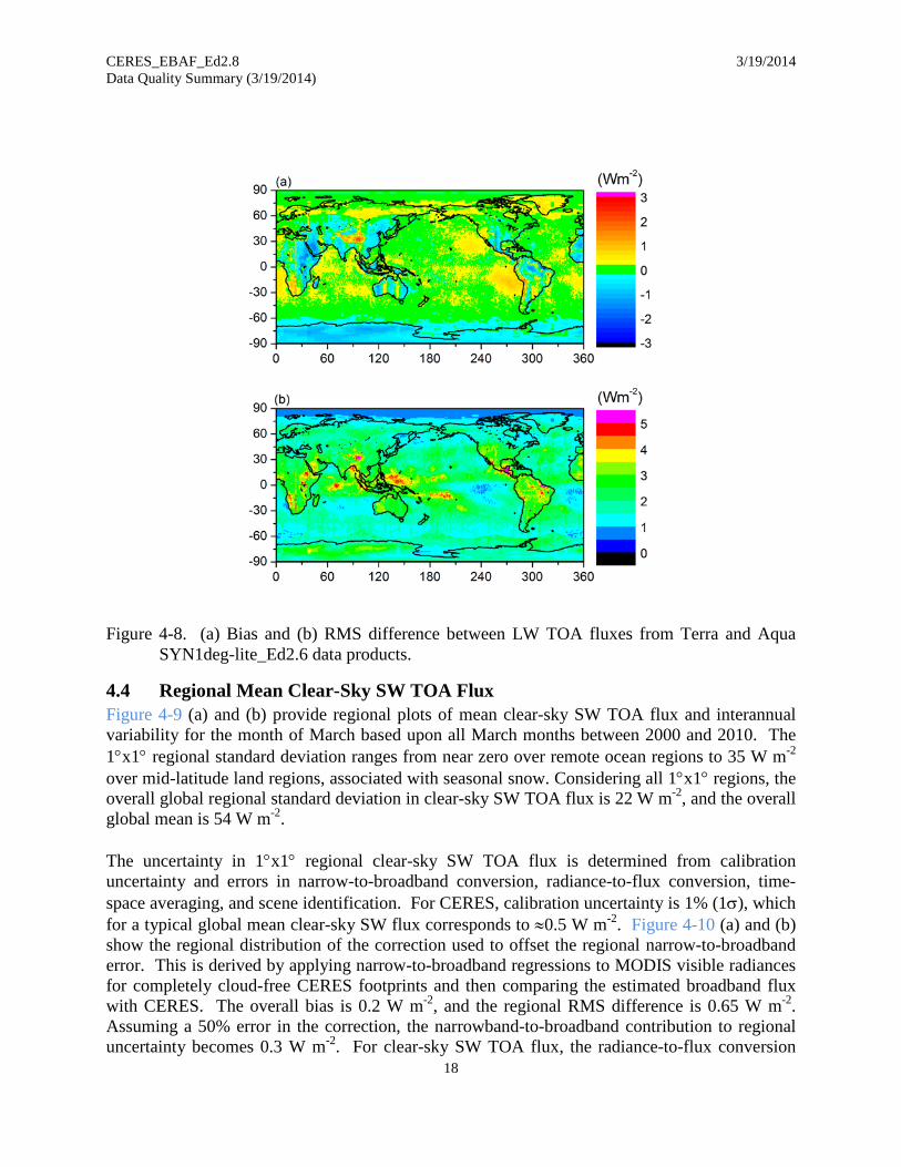
Figure 4-8. (a) Bias and (b) RMS difference between LW TOA fluxes from Terra and Aqua SYN1deg-lite_Ed2.6 data products. ....................................................................... 18

Figure 4-9. (a) Average and (b) standard deviation of clear-sky SW TOA flux determined from all March months from 2000-2010 using the CERES EBAF Ed2.6 product. ................................................................................................................... 19

Figure 4-10. (a) Bias and (b) RMS difference between high-resolution clear-sky SW TOA fluxes derived with and without corrections for regional narrow-to-broadband error. ....................................................................................................................... 20

Figure 4-11. (a) Average and (b) standard deviation of clear-sky LW TOA flux determined from all March months from 2000-2010 using the CERES EBAF Ed2.6 product. ................................................................................................................... 21



iv

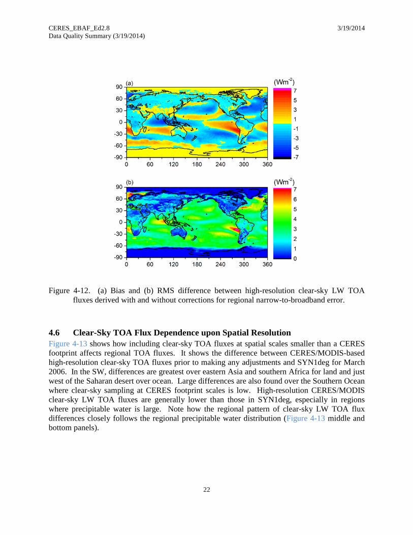
Figure 4-12. (a) Bias and (b) RMS difference between high-resolution clear-sky LW TOA fluxes derived with and without corrections for regional narrow-to-broadband error. ....................................................................................................................... 22

Figure 4-13. Clear-sky TOA flux difference between high resolution CERES/MODIS and SYN1deg-lite_Ed2.5 for SW (top) and LW (middle). Bottom panel shows precipitable water in cm. ........................................................................................ 23

Figure 4-14. Daily total solar irradiance (TSI) used in EBAF Ed2.8 from March 2000 through October 2013 (W m-2). .............................................................................. 25

Figure 4-15. Global monthly mean solar incoming flux in EBAF Ed2.8 from March 2000 through October 2013 (W m-2). .............................................................................. 26

Figure 4-16. Deseasonalized global monthly mean solar incoming flux in EBAF Ed2.8 from March 2000 through October 2013 (W m-2). ......................................................... 26

Figure 5-1. Difference in daily total solar irradiance (TSI) between EBAF Ed2.8 and EBAF Ed2.7 from March 2000 through June 2013 (W m-2). ............................................ 28

Figure 5-2. Difference in global monthly mean solar incoming flux between EBAF Ed2.8 and EBAF Ed2.7 from March 2000 through June 2013 (W m-2). .......................... 28

Figure 5-3. TOA LW CRE for April 2000 from (a) EBAF Ed2.6r and (b) EBAF Ed2.7. ....... 29

Figure 5-4. Regional anomalies in (a) clear-sky SW TOA flux (W m-2) and (b) snow/ice percent coverage (%) for March 2002 from EBAF Ed2.7. .................................... 30

Figure 5-5. February 2003 monthly mean clear-sky SW TOA flux for (a) CERES Terra SSF1deg-lite_Ed2.6, (b) EBAF Ed2.6r, (c) EBAF Ed2.7, and (d) EBAF Ed2.7 minus EBAF Ed2.6r. Units in W m-2. .................................................................... 32

Figure 5-6. February 2003 monthly mean clear-sky LW TOA flux for (a) CERES Terra SSF1deg-lite_Ed2.6, (b) EBAF Ed2.6r, (c) EBAF Ed2.7, and (d) EBAF Ed2.7 minus EBAF Ed2.6r. Units in W m-2. .................................................................... 33

Figure 5-7. (a) Monthly mean daytime-only cloud fraction, (b) daytime-only minus day+night monthly mean cloud fraction, and (c) snow/ice percent coverage. All maps are for February 2003. Units in %. ......................................................... 34

Figure 5-8. Monthly clear-sky SW TOA flux anomalies for (a) 30°S-30°N and (b) global..... 35

Figure 5-9. Monthly clear-sky LW TOA flux anomalies for (a) 30°S-30°N and (b) global. ... 35



v

Figure 5-10. All-sky (a) SW and (b) LW TOA flux difference between EBAF Ed2.7 and EBAF Ed2.6r. ......................................................................................................... 37

Figure 5-11. (a) EBAF Ed2.6 minus EBAF Ed2.6r global mean solar irradiance difference; (b) Anomalies in solar irradiance from EBAF Ed2.6 and EBAF Ed2.6r. .............. 38

Figure 5-12. Anomaly of clear-sky LW TOA flux difference between (a) EBAF Ed2.6 and SSF1deg-lite_Ed2.6 for March 2000–December 2010 and (b) EBAF Ed2.6r and SSF1deg-lite_Ed2.6 for March 2000–June 2011. ........................................... 39


LIST OF TABLES Table Page

vi

Table 2-1. CERES processing level descriptions. ........................................................................ 2

Table 4-1. Global mean TOA fluxes (W m-2) from EBAF Ed1.0, EBAF Ed2.5, EBAF Ed2.6, EBAF Ed2.6r, EBAF Ed2.7 and EBAF Ed2.8 for March 2000-February 2005 and March 2000-February 2010. ............................................... 9

Table 4-2. TSI data sets used in CERES EBAF Ed2.8 ............................................................... 25

Table 5-1. EBAF Input and Heating Rate Constraint. ................................................................ 27

Table 5-2. Slope of least-square regression fit (W m-2 per decade) to monthly anomalies in SW and LW clear-sky TOA flux for March 2000-June 2012. .............................. 36


1

1.0 Introduction CERES instruments fly on the Terra (descending sun-synchronous orbit with an equator crossing time of 10:30 A.M. local time) and Aqua (ascending sun-synchronous orbit with an equator crossing time of 1:30 P.M. local time) satellites. Each CERES instrument measures filtered radiances in the shortwave (SW; wavelengths between 0.3 and 5 µm), total (TOT; wavelengths between 0.3 and 200 µm), and window (WN; wavelengths between 8 and 12 µm) regions. Unfiltered SW, longwave (LW) and WN radiances are determined following Loeb et al. (2001). CERES instruments provide global coverage daily, and monthly mean regional fluxes are based upon complete daily samples over the entire globe. Despite recent improvements in satellite instrument calibration and the algorithms used to determine SW and LW outgoing top-of-atmosphere (TOA) radiative fluxes, a sizeable imbalance persists in the average global net radiation at the TOA from CERES satellite observations. With the most recent CERES Edition3 Instrument calibration improvements, the SYN1deg_Edition3 net imbalance is ~3.4 W m-2, much larger than the expected observed ocean heating rate ~0.58 W m-2 (Loeb et al. 2012a). This imbalance is problematic in applications that use Earth Radiation Budget (ERB) data for climate model evaluation, estimations of the Earth's annual global mean energy budget, and studies that infer meridional heat transports. The CERES Energy Balanced and Filled (EBAF) dataset uses an objective constrainment algorithm to adjust SW and LW TOA fluxes within their ranges of uncertainty to remove the inconsistency between average global net TOA flux and heat storage in the Earth-atmosphere system. A second problem users of standard CERES Level-3 data have noted is the occurrence of gaps in monthly mean clear-sky TOA flux maps due to the absence in some 1°x1° regions of cloud-free areas occurring at the CERES footprint scale (~20-km at nadir). As a result, clear-sky maps from CERES SSF1deg contain many missing regions. In EBAF, the problem of gaps in clear-sky TOA flux maps is addressed by inferring clear-sky fluxes from both CERES and Moderate Resolution Imaging Spectrometer (MODIS) measurements to produce a new clear-sky TOA flux climatology that provides TOA fluxes in each 1°x1° region every month. We urge users to visit the new CERES Data subsetting/visualization/ordering tool, which provides a vastly improved user interface and a wider range of data formats (e.g., ASCII, netCDF) than is available with the ASDC ordering tool, which is limited to HDF. http://ceres.larc.nasa.gov/order_data.php



2

2.0 Description The CERES EBAF Edition2.8 (Ed2.8) product is the culmination of several processing steps, as summarized in Table 2-1. Here we use the latest CERES gains and time-dependent spectral response function values (Thomas et al. 2010; Loeb et al. 2012b). To correct for the imperfect spectral response of the instrument, the filtered radiances are converted to unfiltered SW, LW and WN radiances (Loeb et al. 2001). Since there is no LW channel on CERES, LW daytime radiances are determined from the difference between the TOT and SW channel radiances. Instantaneous TOA radiative fluxes are estimated from unfiltered radiances using empirical angular distribution models (ADMs; Loeb et al. 2003, 2005) for different scene types identified using retrievals from MODIS measurements (Minnis et al. 2011). Their accuracy has been evaluated in several articles (Loeb et al. 2006; Loeb et al. 2007; Kato and Loeb 2005). Monthly mean fluxes are determined by spatially averaging the instantaneous values on a 1°×1° grid, temporally interpolating between observed values at 1-h increments for each hour of every month, and then averaging all hour boxes in a month (Young et al. 1998; Doelling et al. 2013). Level-3 processing is performed on a nested grid, which uses 1° equal-angle regions between 45°N and 45°S, maintaining area consistency at higher latitudes. The fluxes from the nested grid are then output to a complete 360x180 1°×1° grid using replication.

Table 2-1. CERES processing level descriptions.

Level Description 0 Raw digitized instrument data for all engineering and science data streams in

Consultative Committee for Space Data Systems (CCSDS) packet format. 1 Instantaneous filtered broadband radiances at the CERES footprint resolution,

geolocation and viewing geometry, solar geometry, satellite position and velocity, and all raw engineering and instrument status data.

2 Instantaneous geophysical variables at the CERES footprint resolution. Includes some Level 1B parameters and retrieved or computed geophysical variables. (e.g., filtered and unfiltered radiances, viewing geometry, radiative fluxes, imager cloud and aerosol properties)

3 Radiative fluxes and cloud properties spatially averaged onto a uniform grid. Includes either instantaneous averages sorted by local/GMT hour (e.g., SSF1deg–Hour) or temporally interpolated averages at 3–hourly, daily, monthly or monthly hourly intervals (e.g., SSF1deg–Month).

3B Level 3 data products adjusted within their range of uncertainty to satisfy known constraints (e.g., consistency between average global net TOA flux imbalance and ocean heat storage).


3

CERES_EBAF_Ed2.6r, Ed2.7, and Ed2.8 differ from previous versions of EBAF (EBAF Ed1.0, Ed2.5) in that they are based upon two data products differentiated by the interpolation methods used: (i) SSF1deg: The LW fluxes in each hour box between CERES observations are determined by

linear interpolation of LW fluxes over ocean, while daytime and nighttime observations over land and desert are interpolated by fitting a half-sine curve to the observations to account for the much stronger diurnal cycle over land and desert (Young et al. 1998). The SW radiative fluxes between CERES observation times are determined from the observed fluxes by using scene-dependent diurnal albedo models, which describe how TOA albedo (and therefore flux) changes with solar zenith angle for each local time, assuming the scene properties remain invariant throughout the day. The sun angle–dependent diurnal albedo models are based upon the CERES ADMs developed for the Tropical Rainfall Measuring Mission (TRMM) satellite (Loeb et al. 2003).

(ii) SYN1deg: SW and LW radiative fluxes between CERES observation times are determined

by supplementing the CERES observations with 3-hourly TOA fluxes derived from five geostationary satellites. Doelling et al. (2013) provides a detailed description of how broadband TOA fluxes are derived from geostationary data.

SSF1deg provides global coverage daily with excellent calibration stability, but samples only at specific times of the day due to the sun-synchronous orbit. While the SYN1deg approach provides improved diurnal coverage by merging CERES and 3-hourly geostationary data, artifacts in the GEO data over certain regions and time periods can introduce larger uncertainties. In order to remove most of the GEO-derived flux biases, the fluxes are normalized at Terra or Aqua observation times to remain consistent with the CERES instrument calibration (Doelling et al. 2013). Nevertheless, spurious jumps in the SW TOA flux record can still occur when GEO satellites are replaced, due to changes in satellite position, calibration, visible sensor spectral response, and imaging schedules. Such artifacts in the GEO data can be problematic in studies of TOA radiation interannual variability and/or trends. To maintain the excellent CERES instrument calibration stability of SSF1deg and also preserve the diurnal information found in SYN1deg, EBAF Ed2.6r through Ed2.8 use a new approach involving scene dependent diurnal corrections to convert daily regional mean SSF1deg SW fluxes to diurnally complete values analogous to SYN1deg, but without geostationary artifacts. The diurnal corrections are ratios of SYN1deg-to-SSF1deg fluxes defined for each of the five geostationary satellite domains for each calendar month. They depend upon surface type and MODIS cloud fraction and height retrievals, and thus can vary from one day to the next along with the cloud properties (i.e., they are dynamic). For March 2000-June 2002, TOA fluxes are based upon CERES observations from the Terra spacecraft, while for July 2002 onwards, CERES SW observations from both Terra and Aqua are utilized in order to improve the accuracy of the diurnal corrections. In EBAF Ed1.0 and EBAF Ed2.5, only Terra data were used and the main input was either CERES SRBAVG GEO Ed2D or CERES SYN Ed2.5, which both explicitly rely on GEO for time interpolation. All-sky LW TOA fluxes in EBAF Ed2.6r, Ed2.7, and Ed2.8 are derived from internal versions of


4

SYN1deg determined for Terra only. In SYN1deg, LW radiative fluxes between CERES observation times are determined by supplementing the CERES observations with data from 5 geostationary satellites that sample every 3 hours for all longitudes between 60°S and 60°N, thus providing the most temporally and spatially complete CERES dataset for Terra or Aqua. Doelling et al. (2013) provides a detailed description of how broadband TOA fluxes are derived from geostationary data and combined with CERES observations. The approach used to determine clear-sky TOA flux is described in detail in Loeb et al. (2009). We determine gridbox mean clear-sky fluxes using an area-weighted average of: (i) CERES/Terra broadband fluxes from completely cloud-free CERES footprints (20-km equivalent diameter at nadir), and (ii) MODIS/Terra-derived “broadband” clear-sky fluxes estimated from the cloud-free portions of partly and mostly cloudy CERES footprints. In both cases, clear regions are identified using the CERES cloud algorithm applied to MODIS 1-km pixel data (Minnis et al. 2011). Clear-sky fluxes in partly and mostly cloudy CERES footprints are derived using MODIS-CERES narrow-to-broadband regressions to convert MODIS narrowband radiances averaged over the clear portions of a footprint to broadband radiances. In EBAF Ed2.7 and Ed2.8, the SW and LW narrow-to-broadband regressions are developed for each calendar month from all available years of CERES data. In EBAF Ed2.6r, the SW narrow-to-broadband regressions were instead derived for each individual month, which caused larger sampling errors in the regressions, particularly at large solar zenith angles. In both SW and LW, a correction to narrow-to-broadband bias errors is made monthly based upon the difference between broadband radiances for cloud-free CERES footprints and the MODIS-based broadband estimate. This ensures that the final product’s calibration is tied to CERES. The "broadband" MODIS radiances are then converted to TOA radiative fluxes using CERES clear-sky ADMs (Loeb et al. 2005). Despite recent improvements in satellite instrument calibration and the algorithms used to determine CERES TOA radiative fluxes, a sizeable imbalance persists in the average global net radiation at the TOA from CERES satellite observations. As in previous versions of EBAF (Loeb et al. 2009), the CERES SW and LW fluxes in EBAF Ed2.8 are adjusted within their ranges of uncertainty to remove the inconsistency between average global net TOA flux and heat storage in the Earth–atmosphere system, as determined primarily from ocean heat content anomaly (OHCA) data. In the current version, the global annual mean values are adjusted such that the July 2005–June 2010 mean net TOA flux is 0.58±0.38 W m–2 (uncertainties at the 90% confidence level) (Loeb et al. 2012a). The uptake of heat by the Earth for this period is estimated from the sum of: (i) 0.47±0.38 W m–2 from the slope of weighted linear least square fit to ARGO OHCA data (Roemmich et al. 2009) to a depth of 1800 m analyzed following Lyman and Johnson (2008); (ii) 0.07±0.05 W m–2 from ocean heat storage at depths below 2000 m using data from 1981–2010 (Purkey and Johnson 2010), and (iii) 0.04±0.02 W m–2 from ice warming and melt, and atmospheric and lithospheric warming (Hansen et al. 2005; Trenberth 2009).


5

3.0 Cautions and Helpful Hints The CERES Science Team notes several CAUTIONS and HELPFUL HINTS regarding the use of CERES_EBAF_Ed2.8:

• The CERES_EBAF_Ed2.8 product can be visualized, subsetted, and ordered from: http://ceres.larc.nasa.gov.

• A marked trend of -0.6 W m-2 per decade is observed in LW Cloud Radiative Effect (CRE) between March 2000 and February 2013. The CERES team suspects at least part of this trend is spurious. LW CRE is determined from the difference between clear-sky and all-sky TOA fluxes. To determine clear-sky TOA fluxes, a cloud mask is applied to MODIS pixel data in order to distinguish between clear and cloud-contaminated areas. The cloud mask algorithm relies on many ancillary inputs, including output from a meteorological assimilation system. In January 2008, the source of assimilated meteorological data was changed from GEOS-4.1 to GEOS-5.2.0. The CERES team noticed a discontinuity in MODIS-based nighttime cloud fraction after the change, whereas daytime cloud fraction appeared to be unaffected. Since the nighttime cloud mask relies more heavily on assimilated meteorological data than daytime (since no visible MODIS radiances are available at night), the CERES team suspects the nighttime cloud fraction discontinuity is related to the GEOS-4.1 to GEOS-5.2.0 change. While the all-sky LW TOA flux is fairly immune to the GEOS-4 to GEOS-5 change, clear-sky LW fluxes are not, as they depend strongly upon the cloud mask. The CERES team continues to evaluate the impact of the GEOS-4.1 to GEOS-5.2.0 change on clear-sky and all-sky TOA fluxes and plans to update this Data Quality Summary as new information becomes available. This problem will ultimately be resolved in Edition4 (expected to be available in early 2015), which will use a consistent version of meteorological assimilation data throughout the record.

o The SYN1deg product was produced for December 2007 with both versions of GEOS to help users evaluate the impact of the change. SYN1deg is a primary input to the EBAF product. For further information, please visit: http://ceres.larc.nasa.gov/science_information.php?page=Dec2007_GEOS-5.

• The CERES team has significantly reduced the impact of geostationary instrument artifacts in CERES_EBAF_Ed2.7 and Ed2.8 compared to earlier versions (see Section 4.0). However, users are cautioned that in the SW, CERES Terra observations are used for the period from March 2000-June 2002, while both CERES Terra and Aqua are used from July 2002 onwards. Consequently, uncertainties are slightly larger prior to July 2002.

• The solar incoming TOA flux is derived from daily SORCE TIM measurements (see Sections 4.7 and 5.1), which have an average annual flux of ~1361 W m-2, vary with time, and take into account the solar sunspot cycle with an amplitude of ~0.1%.

• Clear-sky TOA fluxes in EBAF Ed2.7 and Ed2.8 are provided for clear regions within CERES footprints from MODIS pixels identified as clear at 1-km spatial resolution. This definition differs from what is used in the standard CERES data products (SSF1deg and SYN1deg), which only provide clear-sky fluxes in regions that are completely cloud-free at the CERES footprint scale. LW TOA fluxes for clear-sky regions identified at the higher

http://ceres.larc.nasa.gov/

http://ceres.larc.nasa.gov/science_information.php?page=Dec2007_GEOS-5


6

spatial resolution are on average 2.4 W m-2 lower overall compared to the coarser resolution footprint case, and the regional RMS difference is 4 W m-2. SW TOA fluxes for clear-sky regions identified at the higher spatial resolution are on average 1.6 W m-2 higher overall compared to the coarser resolution footprint case, and the monthly mean regional RMS difference is 6 W m-2. Users should be aware that both of these definitions of “clear-sky” used for CERES observations might differ from what is used in climate model output. Many models compute clear-sky radiative fluxes in each column, regardless of whether the column is clear or cloudy. Sohn et al. (2006) note that differences in how clear-sky is defined in model output and observations can lead to regional LW TOA flux differences of up to 12 W m-2.

• Clear-sky monthly mean SW and LW TOA fluxes are determined by inferring TOA fluxes at each hour of the month and averaging. SW clear-sky TOA fluxes between observation times are determined from the observed fluxes by using scene-dependent diurnal albedo models to estimate how TOA albedo (and therefore flux) changes with solar zenith angle for each local time, assuming the scene properties remain invariant throughout the day. LW clear-sky TOA fluxes between observation times are determined by linear interpolation of LW fluxes over ocean and by applying a half-sine fit during daytime and nighttime over land and desert. Therefore, for monthly mean clear-sky TOA fluxes, we do not explicitly account for changes in the physical properties of the scene (e.g., aerosols, surface properties) during the course of the day.

• Since TOA flux represents a flow of radiant energy per unit area and varies with distance from the earth according to the inverse-square law, a reference level is also needed to define satellite-based TOA fluxes. From theoretical radiative transfer calculations using a model that accounts for spherical geometry, the optimal reference level for defining TOA fluxes in radiation budget studies for the earth is estimated to be approximately 20 km. At this reference level, there is no need to explicitly account for horizontal transmission of solar radiation through the atmosphere in the earth radiation budget calculation. In this context, therefore, the 20-km reference level corresponds to the effective radiative “top of atmosphere” for the planet. Since climate models generally use a plane-parallel model approximation to estimate TOA fluxes and the earth radiation budget, they implicitly assume zero horizontal transmission of solar radiation in the radiation budget equation and do not need to specify a flux reference level. By defining satellite-based TOA flux estimates at a 20-km flux reference level, comparisons with plane-parallel climate model calculations are simplified since there is no need to explicitly correct plane-parallel climate model fluxes for horizontal transmission of solar radiation through a finite atmosphere. For a more detailed discussion of reference level, please see Loeb et al. (2002).

• When the solar zenith angle is greater than 90°, twilight flux (Kato and Loeb 2003) is added to the outgoing SW flux in order to take into account the atmospheric refraction of light. The magnitude of this correction varies with latitude and season and is determined independently for all-sky and clear-sky conditions. In general, the regional correction is less than 0.5 W m-2, and the global mean correction is 0.2 W m-2. Due to the contribution of twilight, there are regions near the terminator in which outgoing SW TOA flux can exceed the incoming solar radiation. Users should be aware that in these cases, albedos (derived from the ratio of outgoing SW to incoming solar radiation) exceed unity.


7

• EBAF uses geodetic weighting to compute global means. The spherical Earth assumption gives the well-known So/4 expression for mean solar irradiance, where So is the instantaneous solar irradiance at the TOA. When a more careful calculation is made by assuming the Earth is an oblate spheroid instead of a sphere, and the annual cycle in the Earth's declination angle and the Earth-sun distance are taken into account, the division factor becomes 4.0034 instead of 4.

• The following file provides the zonal geodetic weights used to determine global mean quantities. (http://ceres.larc.nasa.gov/science_information.php?page=GeodeticWeights).

http://ceres.larc.nasa.gov/science_information.php?page=GeodeticWeights


8

4.0 Accuracy and Validation

4.1 Global Mean TOA Flux Comparisons CERES_EBAF_Ed2.8 differs from Ed2.7 in the total solar irradiance only; all other fluxes are nearly identical to those in EBAF Ed2.7. Table 4-1 compares global TOA averages for EBAF Ed2.8 with earlier versions of the product. Global mean all-sky TOA fluxes in EBAF Ed2.8 are virtually identical to Ed2.6r, and clear-sky TOA fluxes differ at most by 0.1 W m-2. Regionally, TOA flux differences between Ed2.7/Ed2.8 and Ed2.6r are much larger (see Section 5.0). All-sky SW TOA flux in Ed2.8 is 0.2 W m-2 greater than Ed1.0 and at most 0.1 W m-2 greater than Ed2.5. The main difference between all-sky SW TOA fluxes in EBAF Ed2.8 and Ed2.5 is that Ed2.8 uses the methodology described in Section 2.0 while EBAF Ed2.5 is derived from SYN1deg-lite Ed2.5 (a preliminary release of SYN1deg Ed3), which relies explicitly on geostationary satellite measurements to complete the diurnal cycle. Another difference that applies to all TOA flux variables is that EBAF Ed2.8 applies geodetic weighting when averaging globally, while geocentric weighting is assumed in EBAF Ed2.5 and EBAF Ed1.0.

Clear-sky LW TOA flux in Ed2.8 is 0.2–0.3 W m-2 smaller than Ed2.5 and 3.2 W m-2 smaller than Ed1.0. The difference between EBAF Ed2.8 and Ed2.5 is due to the geodetic versus geocentric weighting discussed above. In EBAF Ed1.0, geocentric weighting is also assumed and the methodology for time-space averaging differs from that in versions Ed2.5 and higher. In EBAF Ed2.5 and higher, monthly mean high-resolution clear-sky SW and LW TOA fluxes are determined using a different time-space averaging technique compared to EBAF Ed1.0. Each day, instantaneous clear-sky TOA fluxes are sorted by local time and averaged over an equal-area 1°×1° latitude-longitude grid. A modified version of the production code used to produce SSF1deg clear-sky fluxes is used to determine monthly mean high-resolution clear-sky SW and LW TOA fluxes. In EBAF Ed1.0, the monthly mean clear-sky TOA fluxes were inferred from daily means without sorting by local time first, resulting in larger uncertainties at mid-to-high latitudes where multiple overpasses per day occur at different local times.


9

Table 4-1. Global mean TOA fluxes (W m-2) from EBAF Ed1.0, EBAF Ed2.5, EBAF Ed2.6, EBAF Ed2.6r, EBAF Ed2.7 and EBAF Ed2.8

for March 2000-February 2005 and March 2000-February 2010.

March 2000–February 2005

Ed1.0 Ed2.5 Ed2.6 Ed2.6r Ed2.7 Ed2.8

Incoming Solar 340.0 340.2 340.5 340.0 340.0 339.9

LW (all-sky) 239.6 239.6 239.9 239.7 239.7 239.6

SW (all-sky) 99.5 99.7 100 99.8 99.8 99.7

Net (all-sky) 0.85 0.85 0.55 0.54 0.57 0.57

LW (clear-sky) 269.1 266.2 266.5 266 265.9 265.9

SW (clear-sky) 52.9 52.4 52.6 52.5 52.6 52.6

Net (clear-sky) 18.0 21.5 21.4 21.5 21.5 21.4

March 2000–February 2010

Ed1.0 Ed2.5 Ed2.6 Ed2.6r Ed2.7 Ed2.8

Incoming Solar 340.1 340.4 339.9 339.9 339.8

LW (all-sky) 239.6 239.9 239.6 239.6 239.6

SW (all-sky) 99.5 99.9 99.7 99.7 99.6

Net (all-sky) 1.0 0.59 0.57 0.59 0.59

LW (clear-sky) 266.0 266.4 265.9 265.8 265.8

SW (clear-sky) 52.4 52.5 52.5 52.6 52.6

Net (clear-sky) 21.6 21.5 21.5 21.5 21.5


10

4.2 Regional Mean All-Sky SW TOA Flux Figure 4-1 (a) and (b) provide regional plots of mean SW TOA flux and interannual variability for EBAF Ed2.6 for the month of March based upon all March months between 2000 and 2010. Similar results are obtained for EBAF Ed2.8 (not shown). The 1°x1° regional standard deviation ranges from near zero at the poles to 40 W m-2 in the western tropical Pacific Ocean region. Considering all 1°x1° regions, the overall global regional standard deviation in SW TOA flux is 22 W m-2, and the overall global mean SW TOA flux is 99.7 W m-2. The uncertainty in 1°x1° regional SW TOA flux is evaluated separately for 03/2000-06/2002 (Terra-Only period) and for 07/2002-12/2010 (Terra-Aqua period). To determine uncertainties for the Terra-Only period, we use data from the Terra-Aqua period and compare regional fluxes derived by applying diurnal corrections to fluxes from Terra SSF1deg with regional fluxes derived by averaging fluxes from Terra and Aqua determined using the SYN1deg interpolation method. SYN1deg combines CERES observations on Terra or Aqua with five geostationary instruments covering all longitudes between 60°S and 60°N, thus providing the most temporally and spatially complete CERES dataset for Terra or Aqua. Figure 4-2 (a) and (b) show maps of the regional bias and RMS error. Here we used SSF1deg-lite_Ed2.6 and SYN1deg-lite_Ed2.6, which are similar to the publically available SYN1deg_and SSF1deg Edition3 data products, which have replaced the former. The overall regional RMS error is 4 W m-2. In stratocumulus regions, RMS differences are typically around 5 W m-2, or approximately 5% of the regional mean value. Uncertainties for the Terra-Aqua period are determined by comparing regional fluxes derived by applying diurnal corrections to the average of Terra and Aqua SSF1deg fluxes with average Terra and Aqua regional fluxes from SYN1deg. Results, in Figure 4-3 (a) and (b), show much improvement over the Terra-only case in Figure 4-2, with regional errors decreasing to 2.7 W m-2 overall and with errors less than 3 W m-2 in stratocumulus regions. To place the above results into context, regional mean and RMS differences between Terra and Aqua SYN1deg SW TOA fluxes are provided in Figure 4-4 (a) and (b). Overall, the RMS difference is 4.4 W m-2. RMS differences greater than 10 W m-2 are evident over Africa, Tibet, and over isolated regions in the Americas. Since the same geostationary data are used for both Terra and Aqua SYN1deg, why should there be any discrepancy? The regional discrepancies are mainly associated with the regional normalization of 3-hourly geostationary data to either Terra or Aqua CERES measurements. The time mismatch of up to 1.5 hours could cause differences in cloud conditions between the two measurements (Doelling et al. 2013). Consequently, a longitudinal striping pattern appears that is correlated with the time separation between the geostationary and sun-synchronous observations. If we assume the overall uncertainty is due to: 1) the EBAF diurnal correction, 2) the combined sum of the Terra and Aqua SYN1deg SW regional fluxes, which is given by the RMS difference between Terra and Aqua SYN1deg divided by the square root of 2, and 3) CERES instrument calibration uncertainty of 1 W m-2 (1σ), the regional uncertainty of all-sky SW TOA flux for EBAF Ed2.8 for March 2000–June 2002 is estimated as sqrt(42+4.42/2 +12) or approximately 5 W m-2, and for July 2002-December 2010 is estimated as sqrt(2.72+4.42/2 +12) or approximately 4 W m-2.


11

While the diurnal corrections applied to SSF1deg fluxes do introduce a slight increase in regional SW TOA flux uncertainty, they dramatically improve the EBAF record by minimizing the impact of geostationary satellite artifacts, especially with respect to temporal regional trends. As an example, Figure 4-5 (a) and (b) show regional trends in SW TOA flux from EBAF Ed2.6 and SYN1deg for March 2000–December 2010. In Figure 4-5b, vertical lines corresponding to geostationary satellite boundaries are clearly visible around 30°E, 100°E, 180°E, 105°W and 40°W. The geostationary artifacts are more pronounced over Africa and Asia but also show up to the east of South America. In contrast, the geostationary artifacts are largely absent in Figure 4-5a, which is based upon EBAF Ed2.6 data. Figure 4-6 provides SW TOA flux anomaly differences between SYN1deg and SSF1deg as well as EBAF and SSF1deg for 60°S-60°N (Figure 4-6a) and for the same latitude range but with longitude restricted to 101.5°E–140°E (Figure 4-6b). The latter region covers much of the Western Tropical Pacific Ocean region, Indonesia, and East Asia. In both cases, the SYN1deg results show a sharp decline relative to SSF1deg reaching 0.4 W m-2 per decade for 60°S-60°N and 1.8 W m-2 per decade in the smaller region. In contrast, the EBAF Ed2.6 results remain well within 0.1 W m-2 per decade of SSF1deg for both cases while still accounting for the diurnal cycle.

Figure 4-1. (a) Average and (b) standard deviation of SW TOA flux determined from all March

months from 2000-2010 using the CERES EBAF Ed2.6 product.


12

Figure 4-2. (a) Bias and (b) RMS difference between SW TOA fluxes derived by applying

diurnal corrections to Terra SSF1deg-lite_Ed2.6 and TOA fluxes from the average of Terra and Aqua SYN1deg-lite.


13

Figure 4-3. Same as Figure 4-2 but after applying diurnal corrections to combined Terra+Aqua

SSF1deg-lite_Ed2.6 fluxes.


14

Figure 4-4. (a) Mean and (b) RMS difference between SW TOA fluxes from CERES Terra and

CERES Aqua SYN1deg-lite_Ed2.6 data products.


15

(a)

(b)

Figure 4-5. Regional trends (W m-2 per decade) in SW TOA flux for March 2000-December

2010 from (a) EBAF Ed2.6 and (b) SYN1deg-lite_Ed2.6.


16

Figure 4-6. SW TOA flux anomaly difference between SYN1deg-lite_Ed2.6 and SSF1deg-

lite_Ed2.6 and between EBAF and SSF1deg-lite_Ed2.6 for (a) 60°S-60°N, and (b) the western sector of the region covered by GMS-5, GOES-9, and MTSAT-1R geostationary satellites (60°S-60°N, 101.5°E-140°E) for July 2002-December 2010. Straight lines correspond to least square fits through the anomaly difference curves. Slopes are in units of W m-2 per decade.

4.3 Regional Mean All-Sky LW TOA Flux Figure 4-7 (a) and (b) provide regional plots of mean LW TOA flux and interannual variability for the month of March based upon all March months between 2000 and 2010. The regional standard deviation ranges from near zero at the poles to 30 W m-2 in the equatorial Pacific Ocean region. Considering all 1°x1° regions between 90°S×90°N, the overall regional standard deviation in LW TOA flux is 17 W m-2, and the overall global mean LW TOA flux is 238 W m-2. The uncertainty in 1°x1° regional LW TOA flux is evaluated using data from 07/2002-12/2010, when CERES instruments on both Terra and Aqua were operating. We compare regional fluxes from Terra and Aqua SYN1deg directly in Figure 4-8 (a) and (b). The overall mean difference is 0.05 W m-2, and the regional RMS difference is 2 W m-2. Regional differences can reach 5 W m-2 in isolated regions of convection over south and central Africa and in the west Pacific Ocean region (Figure 4-8b).


17

Figure 4-7. (a) Average and (b) standard deviation of LW TOA flux determined from all March

months from 2000-2010 using the CERES EBAF Ed2.6 product.


18

Figure 4-8. (a) Bias and (b) RMS difference between LW TOA fluxes from Terra and Aqua

SYN1deg-lite_Ed2.6 data products.

4.4 Regional Mean Clear-Sky SW TOA Flux Figure 4-9 (a) and (b) provide regional plots of mean clear-sky SW TOA flux and interannual variability for the month of March based upon all March months between 2000 and 2010. The 1°x1° regional standard deviation ranges from near zero over remote ocean regions to 35 W m-2 over mid-latitude land regions, associated with seasonal snow. Considering all 1°x1° regions, the overall global regional standard deviation in clear-sky SW TOA flux is 22 W m-2, and the overall global mean is 54 W m-2. The uncertainty in 1°x1° regional clear-sky SW TOA flux is determined from calibration uncertainty and errors in narrow-to-broadband conversion, radiance-to-flux conversion, time-space averaging, and scene identification. For CERES, calibration uncertainty is 1% (1σ), which for a typical global mean clear-sky SW flux corresponds to ≈0.5 W m-2. Figure 4-10 (a) and (b) show the regional distribution of the correction used to offset the regional narrow-to-broadband error. This is derived by applying narrow-to-broadband regressions to MODIS visible radiances for completely cloud-free CERES footprints and then comparing the estimated broadband flux with CERES. The overall bias is 0.2 W m-2, and the regional RMS difference is 0.65 W m-2. Assuming a 50% error in the correction, the narrowband-to-broadband contribution to regional uncertainty becomes 0.3 W m-2. For clear-sky SW TOA flux, the radiance-to-flux conversion


19

error contributes 1 W m-2 to regional RMS error (Loeb et al. 2007), and time-space averaging adds 2 W m-2 uncertainty. The latter is based upon an estimate of the error from TRMM-derived diurnal albedo models that provide albedo dependence upon scene type (Loeb et al. 2003). In EBAF, “clear-sky” is defined as cloud-free at the MODIS pixel scale (1 km). A pixel is identified as clear using spectral MODIS channel information and a cloud mask algorithm (Minnis et al. 2011). Based upon a comparison of SW TOA fluxes for CERES footprints identified as clear according to MODIS but cloudy according to CALIPSO with TOA fluxes from footprints identified as clear according to both MODIS and CALIPSO, Sun et al. (2011) found that footprints with undetected subvisible clouds reflect 2.5 W m-2 more SW radiation compared to completely cloud-free footprints and occur in approximately 50% of footprints identified as clear by MODIS. This implies an error of 1.25 W m-2 due to misclassification of clear scenes. The total error in TOA outgoing clear-sky SW radiation in a region is estimated as sqrt(0.52+0.32+12+22+1.252) or approximately 2.6 W m-2.

Figure 4-9. (a) Average and (b) standard deviation of clear-sky SW TOA flux determined from

all March months from 2000-2010 using the CERES EBAF Ed2.6 product.


20

Figure 4-10. (a) Bias and (b) RMS difference between high-resolution clear-sky SW TOA fluxes

derived with and without corrections for regional narrow-to-broadband error.

4.5 Regional Mean Clear-Sky LW TOA Flux Figure 4-11 (a) and (b) provide regional plots of mean clear-sky LW TOA flux and interannual variability for the month of March based upon all March months between 2000 and 2010. The 1°x1° regional standard deviation ranges from near zero at the poles to 30 W m-2 in mountainous regions. Considering all 1°x1° regions, the overall global regional standard deviation in clear-sky LW TOA flux is 10 W m-2, and the overall global mean clear-sky LW TOA flux is 264 W m-2. The uncertainty in 1°x1° regional clear-sky LW TOA flux is determined from calibration uncertainty and errors in narrow-to-broadband conversion, radiance-to-flux conversion, time-space averaging, and scene identification. For CERES, calibration uncertainty is 0.5% (1σ), which for a typical global mean clear-sky LW flux corresponds to ≈1 W m-2. Figure 4-12 (a) and (b) show the regional distribution of the correction used to offset the regional narrow-to-broadband error. This is derived by applying narrow-to-broadband regressions to MODIS infrared radiances for completely cloud-free CERES footprints and then comparing the estimated broadband flux with CERES. The overall bias is -0.5 W m-2, and the regional RMS difference is 2.5 W m-2. Assuming a 50% error in the correction, the narrowband-to-broadband contribution to regional uncertainty becomes 1.74 W m-2. For clear-sky LW TOA flux, the radiance-to-flux conversion error contributes 0.7 W m-2 to regional RMS error (Loeb et al. 2007), and time-space averaging adds 1 W m-2 uncertainty. The latter assumes zero error over ocean (i.e., no appreciable diurnal cycle in clear-sky LW) and a 3 W m-2 error in the half-sine fit over land and


21

desert (Young et al. 1998). In EBAF, “clear-sky” is defined as cloud-free at the MODIS pixel scale (1 km). A pixel is identified as clear using spectral MODIS channel information and a cloud mask algorithm (Minnis et al. 2011). Based upon a comparison of LW TOA fluxes for CERES footprints identified as clear according to MODIS but cloudy according to CALIPSO with TOA fluxes from footprints identified as clear according to both MODIS and CALIPSO, Sun et al. (2011) found that footprints with undetected subvisible clouds emit 5.5 W m-2 less LW radiation compared to completely cloud-free footprints and occur in approximately 50% of footprints identified as clear by MODIS. This implies an error of 2.75 W m-2 due to misclassification of clear scenes. The total error in TOA outgoing clear-sky LW radiation in a region is estimated as sqrt(12+1.742+0.72+12+2.752) or approximately 3.6 W m-2.

Figure 4-11. (a) Average and (b) standard deviation of clear-sky LW TOA flux determined from

all March months from 2000-2010 using the CERES EBAF Ed2.6 product.


22

Figure 4-12. (a) Bias and (b) RMS difference between high-resolution clear-sky LW TOA

fluxes derived with and without corrections for regional narrow-to-broadband error.

4.6 Clear-Sky TOA Flux Dependence upon Spatial Resolution Figure 4-13 shows how including clear-sky TOA fluxes at spatial scales smaller than a CERES footprint affects regional TOA fluxes. It shows the difference between CERES/MODIS-based high-resolution clear-sky TOA fluxes prior to making any adjustments and SYN1deg for March 2006. In the SW, differences are greatest over eastern Asia and southern Africa for land and just west of the Saharan desert over ocean. Large differences are also found over the Southern Ocean where clear-sky sampling at CERES footprint scales is low. High-resolution CERES/MODIS clear-sky LW TOA fluxes are generally lower than those in SYN1deg, especially in regions where precipitable water is large. Note how the regional pattern of clear-sky LW TOA flux differences closely follows the regional precipitable water distribution (Figure 4-13 middle and bottom panels).


23

Figure 4-13. Clear-sky TOA flux difference between high resolution CERES/MODIS and

SYN1deg-lite_Ed2.5 for SW (top) and LW (middle). Bottom panel shows precipitable water in cm.


24

4.7 Solar Incoming The CERES science team provides monthly regional mean TOA incident shortwave radiation derived from the Total Solar Irradiance (TIM) instrument aboard the Solar Radiation and Climate Experiment (SORCE) satellite. The TIM instrument measures the absolute intensity of solar radiation, integrated over the entire solar disk and the entire solar spectrum reported at the mean solar distance of 1 astronomical unit (AU). The CERES product uses the daily total solar irradiance (TSI) product from SORCE, which can be accessed at this web site: http://lasp.colorado.edu/data/sorce/tsi_data/daily/sorce_tsi_L3_c24h_latest.txt. The TIM Total Solar Irradiance (TSI) measurements monitor the incident sunlight to the Earth's atmosphere using an ambient temperature active cavity radiometer. Using electrical substitution radiometers (ESRs) and taking advantage of new materials and modern electronics, the TIM measures TSI to an estimated absolute accuracy of 350 ppm (0.035%). Relative changes in solar irradiance are measured to less than 10 ppm/yr (0.001%/yr), allowing determination of possible long-term variations in the Sun's output (Kopp et al. 2005). Since CERES has a longer data record than SORCE TIM, the daily TSI incorporated by CERES is a combination of several datasets (Table 4-2). A plot of the combined daily TSI is shown in Figure 4-14. The corresponding EBAF Ed2.8 global monthly mean solar incoming flux is shown in Figure 4-15 with deseasonalized values in Figure 4-16. The daily TSI that EBAF uses can be obtained at this web site: http://ceres.larc.nasa.gov/science_information.php?page=TSIdata. The SORCE TIM instrument stopped collecting daily TSI after a battery failure that occurred on the SORCE satellite on July 30, 2013. A new operational mode was implemented on February 24, 2014 in order to provide overlap with the Total solar irradiance Calibration Transfer Experiment (TCTE)/TIM, which was launched on November 19, 2013, although the data is of lower quality. The CERES EBAF Edition 2.8 TSI calibration is referenced to SORCE TSI V-15. Any temporal updates to the TSI will be based on the V-15 calibration. The updated daily TSI will be radiometrically scaled during a 5-year period (01Mar2003 - 29Feb2008).

http://lasp.colorado.edu/data/sorce/tsi_data/daily/sorce_tsi_L3_c24h_latest.txt

http://ceres.larc.nasa.gov/science_information.php?page=TSIdata


25

Table 4-2. TSI data sets used in CERES EBAF Ed2.8

Period TSI Source March 1, 2000 – February 24, 2003

From Dr. Greg Kopp of LASP, University of Colorado, Boulder, who had extracted it from a composite dataset from the World Radiation Center (WRC), Davos. The file used, "composite_d41_62_0906.dat" was downloaded from the ftp site: ftp://ftp.pmodwrc.ch/pub/data/irradiance/composite. Dr. Kopp had offset WRC-Composite time series to match with the SORCE version available at the time (V-09). We offset the WRC-Composite time series further to match with SORCE V-15 data following the procedure suggested by Dr. Kopp. According to this procedure, the offset between the SORCE time series and another one is determined by comparing the two time series for the period 25Feb2003 to 31Dec2003.

February 25, 2003 – June 30, 2013

SORCE TIM V-15 (Kopp and Lean 2011)

July 1, 2013 -- present

A composite data set available from the Royal Meteorological Institute of Belgium (RMIB) (Mekaoui and Dewitte 2008). It is based on the DIARAD/VIRGO data set (Dewitte et al. 2004) and absolutely calibrated according to Dewitte et al. 2013. This data set was radiometrically scaled to SORCE TIM V-15 using an offset, which was determined over a 5-year period (01Mar2003 - 29Feb2008).

Figure 4-14. Daily total solar irradiance (TSI) used in EBAF Ed2.8 from March 2000 through

October 2013 (W m-2).


26

Figure 4-15. Global monthly mean solar incoming flux in EBAF Ed2.8 from March 2000

through October 2013 (W m-2).

Figure 4-16. Deseasonalized global monthly mean solar incoming flux in EBAF Ed2.8 from

March 2000 through October 2013 (W m-2).


27

5.0 Version History Summary Table 5-1 provides a list of input data products used to create each version of EBAF and also lists the reference providing the global energy imbalance constraint used to anchor the CERES TOA fluxes.

Table 5-1. EBAF Input and Heating Rate Constraint.

Version SW all-sky LW all-sky Clear-sky Global Energy

Imbalance Constraint

Ed1 Terra-SYN1deg-lite Ed2.0 (SRBAVG)

Terra-SYN1deg-lite Ed2 (SRBAVG)

Terra-SYN1deg-lite Ed2 (SRBAVG)

Hansen 2005

Ed2.5 Terra-SYN1deg-lite Ed2.5

Terra-SYN1deg-lite Ed2.5

Terra-SSF1deg-lite Ed2.5

Hansen 2005

Ed2.6, Ed2.6r

Terra/Aqua-SSF/SYN1deg-lite Ed2.6

Terra-SYN1deg-lite Ed2.6

Terra-SSF1deg-lite Ed2.6

ARGO-based 2006-2010

Ed2.7 Terra/Aqua-SSF/SYN1deg-lite Ed2.7 (internal)

Terra-SYN1deg-lite Ed2.7 (internal)

Terra-SSF1deg-lite Ed2.7 (internal)


Ed2.8 Terra/Aqua-SSF/SYN1deg-lite Ed2.7 (internal)

Terra-SYN1deg-lite Ed2.7 (internal)

Terra-SSF1deg-lite Ed2.7 (internal)


5.1 Difference between EBAF Ed2.8 and EBAF Ed2.7

5.1.1 Solar Incoming The CERES EBAF TSI were not referenced to a single SORCE TIM version prior to Edition 2.8. The daily TSI from SORCE were simply appended to extend the dataset. The SORCE TIM updated from V-10 to V-15 between December 2009 and January 27, 2014 (http://lasp.colorado.edu/home/sorce/data/tsi-data/tim-tsi-release-notes/). Most of the versions had a very small effect on the TIM reference calibration, except between V-13 and V-14 in May 2013, which had a significant impact on the TSI difference as shown in Figure 5-1. The corresponding EBAF Ed2.8 minus Ed2.7 global monthly mean solar incoming flux difference is shown in Figure 5-2. CERES Edition 2.8 TSI will be referenced to SORCE TIM TSI V-15 as described in Section 4.7. Any future updates to the Edition 2.8 daily TSI dataset will be radiometrically scaled to SORCE TIM TSI V-15 in order to ensure consistent solar incoming fluxes in the EBAF dataset.

http://lasp.colorado.edu/home/sorce/data/tsi-data/tim-tsi-release-notes/


28

Figure 5-1. Difference in daily total solar irradiance (TSI) between EBAF Ed2.8 and EBAF

Ed2.7 from March 2000 through June 2013 (W m-2).

Figure 5-2. Difference in global monthly mean solar incoming flux between EBAF Ed2.8 and

EBAF Ed2.7 from March 2000 through June 2013 (W m-2).

5.2 Difference between EBAF Ed2.7 and EBAF Ed2.6r

5.2.1 Clear-Sky

Two major changes were made in determining clear-sky TOA fluxes in EBAF Ed2.7:

1. In EBAF Ed2.6r, clear-sky TOA fluxes over snow and sea-ice surfaces were determined from CERES radiances for completely cloud-free CERES footprints. For all other surface types, CERES clear-sky TOA fluxes were supplemented with fluxes derived from partly cloudy CERES footprints via narrow-to-broadband regression (Loeb et al. 2009). In EBAF Ed2.7, we extend the regression approach to also include partly cloudy CERES


29

footprints over snow and sea-ice. The change significantly improves LW cloud radiative effect (CRE) over regions like Tibet, where there is poor sampling of clear-sky scenes at the CERES footprint scale. To illustrate the difference, Figure 5-3a shows TOA LW CRE for April 2000 from EBAF Ed2.6r. Over the Tibet region, LW CRE in excess of 80 W m-

2 occurs over a large area, which is physically unrealistic. The problem is due to a lack of clear-sky CERES footprints during nighttime that causes the 24-h average clear-sky flux to be dominated by daytime values, leading to an overestimation of clear-sky LW flux and LW CRE. By including TOA fluxes inferred from partly cloudy CERES footprints in EBAF Ed2.7, the clear-sky sampling increases both during daytime and nighttime, resulting in more realistic values (Figure 5-3b). The increased sampling of clear-sky snow/ice regions also results in a better correspondence between regional SW clear-sky TOA flux anomalies and anomalies in snow/sea-ice, as illustrated in Figure 5-4.

Figure 5-3. TOA LW CRE for April 2000 from (a) EBAF Ed2.6r and (b) EBAF Ed2.7.


30

(a)

(b)

Figure 5-4. Regional anomalies in (a) clear-sky SW TOA flux (W m-2) and (b) snow/ice percent

coverage (%) for March 2002 from EBAF Ed2.7.

2. In EBAF Ed2.6r, SW clear-sky narrow-to-broadband regressions based upon CERES and MODIS were derived separately each month, whereas LW regressions were derived for “climatological” months, for example, from all Januaries, Februaries, etc. In EBAF Ed2.7, we have changed how SW regressions are derived so that a consistent approach is used for both SW and LW. To ensure clear-sky narrow-to-broadband errors do not dominate or introduce spurious trends, the high-resolution clear-sky fluxes are corrected after-the-fact each month by subtracting out the narrow-to-broadband error that is derived from the high-resolution minus CERES broadband flux at the CERES footprint scale (Loeb et al. 2009).


31

To help better understand the differences between clear-sky SW TOA fluxes in EBAF Ed2.7 and Ed2.6r, it is helpful to first look at the CERES-only clear-sky TOA flux in SSF1deg (Figure 5-5a). The white areas correspond to regions in which there are no cloud-free CERES footprints identified by the daytime CERES cloud mask, which is shown in Figure 5-7a. EBAF Ed2.6r (Figure 5-5b) samples most of the missing regions because it includes clear-sky fluxes derived from partly cloudy CERES footprints for surfaces that are free from snow and ice. If there remain any unsampled regions, they get filled in using an interpolation scheme that averages surrounding regions with non-default values. EBAF Ed2.7 (Figure 5-5c) looks a lot like Ed2.6r, except near 60°S and over snow/sea-ice regions. The difference map (EBAF Ed2.7 minus EBAF Ed2.6r) is provided in Figure 5-5d. The yellow band near 60°S is due to the change in methodology used to generate the narrow-to-broadband regressions (item (2) above). The narrow-to-broadband regressions derived from just one month in EBAF Ed2.6r suffer from reduced sampling, particularly in the large solar zenith angle (high-latitude) bins. EBAF Ed2.7 has much better sampling since it is based upon all Januaries, Februaries, etc. Differences in Figure 5-5d are also quite large over land between 50°N-60°N (Russia and western Canada). Those regions are very cloudy (Figure 5-7a) and snow covered (Figure 5-7c). In EBAF Ed2.6r these regions were filled by interpolation since they were missing in SSF1deg (Figure 5-5a). In EBAF Ed2.7, clear-sky SW TOA fluxes in these regions are now determined directly from clear-free portions of partly cloudy footprints rather than by interpolation, and thus are more representative of actual conditions. Differences between EBAF Ed2.7 and Ed2.6r clear-sky LW TOA fluxes over snow and sea-ice are also quite pronounced (Figure 5-6d), particularly over snow-covered Russia, Canada, and in mountainous regions of central Asia. This pattern is also apparent in Figure 5-7b, which shows the difference in monthly mean cloud fraction for daytime-only and daytime+nighttime sampling. Figure 5-7b shows that there is more daytime than nighttime cloud over snow-covered Russia and Canada, but less daytime than nighttime cloud cover over the mountainous regions of central Asia (e.g., Tibet). Similarly, SSF1deg clear-sky SW and LW TOA flux maps in Figure 5-5a and Figure 5-6a show marked differences in sampling over Russia, indicating that LW fluxes in SSF1deg and EBAF Ed2.6r are mainly determined from nighttime overpasses due to the absence of daytime clear-sky samples at the CERES footprint scale. Consequently, clear-sky LW fluxes in EBAF Ed2.6r are likely biased low over snow-covered Russia and Canada because clear-sky footprints are obtained mainly at night (there could also be more cloud contamination at night). In contrast, EBAF Ed2.6r clear-sky LW is likely biased high over Tibet since more of the clear-sky samples are obtained during daytime. Because EBAF Ed2.7 now includes clear-sky fluxes from partly cloud footprints, it has a more uniform daytime/nighttime sampling distribution and a smaller regional clear-sky TOA flux bias.


32

(a)

(b)

(c)

(d)

Figure 5-5. February 2003 monthly mean clear-sky SW TOA flux for (a) CERES Terra

SSF1deg-lite_Ed2.6, (b) EBAF Ed2.6r, (c) EBAF Ed2.7, and (d) EBAF Ed2.7 minus EBAF Ed2.6r. Units in W m-2.


33

(a)

(b)

(c)

(d)

Figure 5-6. February 2003 monthly mean clear-sky LW TOA flux for (a) CERES Terra

SSF1deg-lite_Ed2.6, (b) EBAF Ed2.6r, (c) EBAF Ed2.7, and (d) EBAF Ed2.7 minus EBAF Ed2.6r. Units in W m-2.


34

(a)

(b)

(c)

Figure 5-7. (a) Monthly mean daytime-only cloud fraction, (b) daytime-only minus day+night

monthly mean cloud fraction, and (c) snow/ice percent coverage. All maps are for February 2003. Units in %.

As was already shown in Table 4-1, the changes introduced in EBAF Ed2.7 have negligible impact on the global mean values: SW clear-sky global mean fluxes differ by 0.1 W m-2, and there are virtually no changes to all-sky TOA fluxes. Anomalies in large-scale monthly mean clear-sky TOA fluxes in SSF1deg, EBAF Ed2.6r and EBAF Ed2.7 are shown in Figure 5-8 and Figure 5-9 for 30°S-30°N and the globe. Overall the anomalies from the three versions track one another quite closely. The largest differences occur in SW between SSF1deg and the two EBAF versions, particularly at the global scale. Reduced sampling of clear-sky scenes at middle and high latitudes in SSF1deg (e.g., Figure 5-5a) is the likely reason for the larger global clear-sky SW TOA flux anomaly differences. The slopes of linear regression fits to monthly anomaly time-series for different averaging domains is provided in Table 5-2. In EBAF Ed2.7 the SW trend is near zero for the 30°S-30°N and 60°S-60°N domains, and -0.24 W m-2 per decade for the globe due to a marked decline of 2


35

W m-2 per decade poleward of 60°, which is apparent in all three versions. In EBAF Ed2.6r the global SW TOA flux trend is near zero due to compensation between a 0.22 W m-2 per decade trend for 60°S-60°N and the negative trend poleward of 60°. In the LW, trends for the two EBAF versions are consistent to within 0.05 W m-2 per decade in all averaging domains considered.

Figure 5-8. Monthly clear-sky SW TOA flux anomalies for (a) 30°S-30°N and (b) global.

Figure 5-9. Monthly clear-sky LW TOA flux anomalies for (a) 30°S-30°N and (b) global.


36

Table 5-2. Slope of least-square regression fit (W m-2 per decade) to monthly anomalies in SW and LW clear-sky TOA flux for March 2000-June 2012.

SW Clear-Sky TOA Flux “Trend” Domain SSF1deg-lite

Ed2.6 EBAF

Ed2.6r EBAF Ed2.7

30°S−30°N -0.076 0.13 -0.031 60°S−60°N -0.17 0.22 0.045 90°S−90°N -0.45 -0.045 -0.24

60°−90° -2.4 -1.8 -2.0 LW Clear-Sky TOA Flux “Trend”

Domain SSF1deg-lite Ed2.6

EBAF Ed2.6r

EBAF Ed2.7

30°S−30°N -0.97 -0.96 -1.0 60°S−60°N -0.81 -0.88 -0.90 90°S−90°N -0.62 -0.66 -0.69

60°−90° 0.49 0.70 0.65

5.2.2 All-Sky EBAF Ed2.7 corrects a small error in how regional averages are determined for gridboxes that contain footprints from the same overpass that fall in two different local time zones. In EBAF Ed2.6r, only footprints in the last time zone read were used to determine the gridbox average, while EBAF Ed2.7 correctly considers footprints in both time zones. This change has no impact on large-scale averages (Table 4-1), but it does alter regional fluxes every 15° in longitude, corresponding to transitions from one time zone to another (Figure 5-10). In addition, small SW TOA flux regional differences between EBAF Ed2.7 and E2.6r occur as a result of an update to the EBAF SW TOA flux diurnal correction look-up tables used in EBAF Ed2.7. This is the reason for the 0.5 W m-2 differences south of Australia in Figure 5-10a.


37

(a)

(b)

Figure 5-10. All-sky (a) SW and (b) LW TOA flux difference between EBAF Ed2.7 and EBAF

Ed2.6r.

5.3 Difference between EBAF Ed2.6r and EBAF Ed2.6

(a) Global Mean Calculation

In EBAF Ed2.6 a code error in the global mean calculation of all variables was discovered. The root cause was the use of incorrect zonal weights in the integration of global mean quantities. The problem was corrected in EBAF Ed2.6r by using correct zonal weights for an oblate spheroid Earth (http://ceres.larc.nasa.gov/science_information.php?page=GeodeticWeights). Figure 5-11a compares the difference between global mean solar irradiance for EBAF Ed2.6 and EBAF Ed2.6r. Global mean differences exhibit a seasonal cycle with maxima occurring in June and minima in December. The code error does not impact deseasonalized anomalies in global mean quantities, as illustrated in Figure 5-11b.

http://ceres.larc.nasa.gov/science_information.php?page=GeodeticWeights


38

Figure 5-11. (a) EBAF Ed2.6 minus EBAF Ed2.6r global mean solar irradiance difference; (b)

Anomalies in solar irradiance from EBAF Ed2.6 and EBAF Ed2.6r.


39

(b) Clear-sky LW TOA Fluxes

Deseasonalized anomalies in clear-sky LW TOA flux from EBAF Ed2.6 show a marked discontinuity after 2008 relative to anomalies in SSF1deg (Figure 5-12a). The problem is associated with greater sampling uncertainties in the monthly narrow-to-broadband coefficients after 2008 due to a decrease in cloud cover during this period. To overcome this problem, LW narrow-to-broadband regressions are re-derived in EBAF Ed2.6r for each calendar month using all data from March 2000 through June 2011. Monthly regional bias errors are removed using difference maps of broadband and narrow-to-broadband cloud-free TOA fluxes at the CERES footprint scale. This ensures that the final product’s calibration is tied to CERES. After applying this modified approach, anomalies from EBAF Ed2.6r are closer to SSF1deg (Figure 5-12b) and show no discontinuity after 2008. Further, anomalies are less noisy compared to Ed2.6.

Figure 5-12. Anomaly of clear-sky LW TOA flux difference between (a) EBAF Ed2.6 and

SSF1deg-lite_Ed2.6 for March 2000–December 2010 and (b) EBAF Ed2.6r and SSF1deg-lite_Ed2.6 for March 2000–June 2011.


40

5.4 Other Differences Amongst Earlier Versions of EBAF The main impact of the Edition2.5 calibration changes to EBAF is to improve the calibration stability of the record. Another significant difference between EBAF Ed1.0 and Ed2.5 is in clear-sky, particularly in the LW. In EBAF Ed2.5, monthly mean high-resolution clear-sky SW and LW TOA fluxes are determined using a different time-space averaging technique compared to EBAF Ed1.0. Each day, instantaneous clear-sky TOA fluxes are sorted by local time and averaged over an equal-area 1°×1° latitude-longitude grid. A modified version of the production code used to produce CERES SRBAVG and SSF1deg clear-sky fluxes was used to determine monthly mean high-resolution clear-sky SW and LW TOA fluxes in EBAF Ed2.5. In EBAF Ed1.0, the monthly mean clear-sky TOA fluxes were inferred from daily means without sorting by local time first, resulting in larger uncertainties at mid-to-high latitudes where multiple overpasses per day occur at different local times. After the release of SRBAVG-GEO Ed2D, an error was discovered in the computation of the declination angle and earth-sun distance factor. The angle and factor were computed at 00:00 GMT instead of 12:00 GMT, which is appropriate for computing the solar incoming in local time. This has no effect on the annual mean insolation but significantly affects the monthly zonal solar incoming fluxes near the poles. This error is corrected in the final adjusted TOA fluxes and will also be rectified in the next SRBAVG version (Edition3). Adjustments to total solar irradiance associated with the spherical Earth assumption are applied zonally to improve the accuracy of incoming solar radiation at each latitude. While these adjustments are applied at the zonal level, averaged globally the correction is consistent with that in Section 5.2. Similarly, adjustments in SW TOA fluxes due to near-terminator flux biases are also applied zonally without modifying the global mean. Separate adjustments are made for clear and all-sky TOA fluxes.


41

6.0 References The full version of CERES EBAF Ed2.8 is available from the following ordering site: http://ceres.larc.nasa.gov/order_data.php

Dewitte, S., D. Crommelynck, and A. Joukoff, 2004: Total solar irradiance observations from DIARAD/VIRGO. J. Geophys. Res., 109, A02102, doi:10.1029/2002JA009694.

Dewitte, S., E. Janssen, and S. Mekaoui, 2013: Science results from the Sova-Picard total solar irradiance instrument, AIP Conf. Proc., 1531, 688-691, doi:10.1063/1.4804863.

Doelling, D. R., N. G. Loeb, D. F. Keyes, M. L. Nordeen, D. Morstad, C. Nguyen, B. A. Wielicki, D. F. Young, and M. Sun, 2013: Geostationary enhanced temporal interpolation for CERES flux products. J. Atmos. Oceanic Technol., 30, 1072-1090.

Fröhlich, C., and J. Lean, 1998: The Sun's total irradiance: Cycles, trends and related climate change uncertainties since 1976. Geophys. Res. Lett., 25(23), 4377-4380.

Hansen, J. et al. 2005: Earth’s energy imbalance: confirmation and implications. Science, 308, 1431–1435.

Kato, S., and N. G. Loeb, 2003: Twilight irradiance reflected by the earth estimated from Clouds and the Earth’s Radiant Energy System (CERES) measurements. J. Climate, 16, 2646–2650.

Kato, S., and N. G. Loeb, 2005: Top-of-atmosphere shortwave broadband observed radiance and estimated irradiance over polar regions from Clouds and the Earth’s Radiant Energy System (CERES) instruments on Terra. J. Geophys. Res., 110, doi:10.1029/2004JD005308.

Kopp, G. and G. Lawrence, 2005: The Total Irradiance Monitor (TIM): Instrument design. Sol. Phys., 230, 91-109.

Kopp, G. and J. L. Lean, 2011: A new, lower value of total solar irradiance: Evidence and climate significance. Geophys. Res. Lett., 38, L01706, doi:10.1029/2010GL045777.

Loeb, N. G., K. J. Priestley, D. P. Kratz, E. B. Geier, R. N. Green, B. A. Wielicki, P. O. R. Hinton, and S. K. Nolan, 2001: Determination of unfiltered radiances from the Clouds and the Earth’s Radiant Energy System (CERES) instrument. J. Appl. Meteor., 40, 822–835.

Loeb, N. G., S. Kato, and B. A. Wielicki, 2002: Defining top-of-atmosphere flux reference level for Earth Radiation Budget studies. J. Climate, 15, 3301-3309.

Loeb, N. G., N. M. Smith, S. Kato, W. F. Miller, S. K. Gupta, P. Minnis, and B. A. Wielicki, 2003: Angular distribution models for top-of-atmosphere radiative flux estimation from the Clouds and the Earth’s Radiant Energy System instrument on the Tropical Rainfall Measuring Mission Satellite. Part I: Methodology. J. Appl. Meteor., 42, 240–265.

Loeb, N. G., S. Kato, K. Loukachine, and N. M. Smith, 2005: Angular distribution models for top-of-atmosphere radiative flux estimation from the Clouds and the Earth’s Radiant Energy System instrument on the Terra satellite. Part I: Methodology. J. Atmos.



42

Oceanic Technol., 22, 338–351.

Loeb, N. G., W. Sun, W. F. Miller, K. Loukachine, and R. Davies, 2006: Fusion of CERES, MISR and MODIS measurements for top-of-atmosphere radiative flux validation. J. Geophys. Res., 111, D18209, doi:10.1029/2006JD007146.

Loeb, N. G., B. A. Wielicki, W. Su, K. Loukachine, W. Sun, T. Wong, K. J. Priestley, G. Matthews, W. F. Miller, and R. Davies, 2007: Multi-instrument comparison of top-of-atmosphere reflected solar radiation. J. Climate, 20, 575-591.

Loeb, N. G., B. A. Wielicki, D. R. Doelling, G. L. Smith, D. F. Keyes, S. Kato, N. Manalo-Smith, T. Wong, 2009: Toward optimal closure of the Earth’s top-of-atmosphere radiation budget. J. Climate, 22, 748-766, doi:10.1175/2008JCLI2637.1.

Loeb, N. G., J. M. Lyman, G. C. Johnson, R. P. Allan, D. R. Doelling, T. Wong, B. J. Soden, and G. L. Stephens, 2012a: Observed changes in top-of-the-atmosphere radiation and upper-ocean heating consistent within uncertainty. Nat. Geosci., 5, doi:10.1038/NGEO1375.

Loeb, N. G., S. Kato, W. Su, T. Wong, F. G. Rose, D. R. Doelling, J. R. Norris, and X. Huang, 2012b: Advances in understanding top-of-atmosphere radiation variability from satellite observations. Surv. Geophys., 33, 359-385. DOI 10.1007/s10712-012-9175-1.

Lyman, J. M., and G. C. Johnson, 2008: Estimating annual global upper-ocean heat content anomalies despite irregular in situ ocean sampling. J. Climate, 21, 5629–5641.

Mekaoui, S., and S. Dewitte, 2008: Total Solar Irradiance measurement and modelling during cycle 23, Sol. Phys., 247, 203-216.

Minnis P., S. Sun-Mack, D. F. Young, P. W. Heck, D. P. Garber, Y. Chen, D. A. Spangenberg, R. F. Arduini, Q. Z. Trepte, W. L. Smith, Jr., J. K. Ayers, S. C. Gibson, W. F. Miller, G. Hong, V. Chakrapani, Y. Takano, K.-N. Liou, Y. Xie, and P. Yang, 2011: CERES Edition-2 cloud property retrievals using TRMM VIRS and Terra and Aqua MODIS data--Part I: Algorithms. IEEE Trans. Geosci. Remote Sens., 49, 4374-4400.

Purkey, S. G., and G. C. Johnson, 2010: Warming of global abyssal and deep southern ocean waters between the 1990s and 2000s: contributions to global heat and sea level rise budgets. J. Climate, 23, 6336–6351.

Roemmich, D. et al., 2009: Argo: the challenge of continuing 10 years of progress. Oceanography, 22, 46–55.

Sohn, B.-J., J. Schmetz, R. Stuhlmann, and J.-Y. Lee, 2006: Dry bias in satellite-derived clear-sky water vapor and its contribution to longwave cloud radiative forcing. J. Climate, 19, 5570-5580.

Sun, W., N. G. Loeb, S. Kato, B. Lin, Y. Hu, and C. Lukashin, 2011: A study of subvisual clouds and their radiation effect with a synergy of CERES, MODIS, CALIPSO, AIRS, and AMSR-E data. Atmos. Chem. Phys. (submitted).

Thomas S., K. J. Priestley, N. Manalo-Smith, N. G. Loeb, P. C. Hess, M. Shankar, D. R. Walikainen, Z. P. Szewcyzk, R. S. Wilson, D. L. Cooper, 2010: Characterization of the Clouds and the Earth’s Radiant Energy System (CERES) sensors on the Terra and Aqua spacecraft, Proc. SPIE, Earth Observing Systems XV, Vol. 7807, 780702, August 2010.


43

Trenberth, K. E., 2009: An imperative for climate change planning: tracking Earth's global energy. Current Opinion in Environmental Sustainability, 1, 19–27.

Young, D. F., P. Minnis, D. R. Doelling, G. G. Gibson, and T. Wong, 1998: Temporal Interpolation Methods for the Clouds and Earth's Radiant Energy System (CERES) Experiment. J. Appl. Meteorol., 37, 572-590.


44

7.0 Expected Reprocessing The CERES team expects to reprocess the EBAF record once SYN1deg and SSF1deg Edition 4 data products are available. We expect the next reprocessing of EBAF to occur in early 2015. Any updates to the CERES EBAF product will be available for subsetting/visualization/ordering at: http://ceres.larc.nasa.gov/order_data.php.



45

8.0 Attribution When referring to the CERES EBAF product, please include the data product and the data set version as "CERES_EBAF_Ed2.8.” The CERES Team has put forth considerable effort to remove major errors and to verify the quality and accuracy of this data. Please provide a reference to the following paper when you publish scientific results with the CERES EBAF_Ed2.8 Loeb, N. G., B. A. Wielicki, D. R. Doelling, G. L. Smith, D. F. Keyes, S. Kato, N. Manalo-

Smith, T. Wong, 2009: Toward optimal closure of the Earth’s top-of-atmosphere radiation budget. J. Climate, 22, 748-766, doi:10.1175/2008JCLI2637.1.

When CERES data obtained via the CERES web site are used in a publication, we request the following acknowledgment be included: "These data were obtained from the NASA Langley Research Center CERES ordering tool at (http://ceres.larc.nasa.gov/)."

http://ceres.larc.nasa.gov/


46

9.0 Feedback and Questions For questions or comments on the CERES Quality Summary, contact the User and Data Services staff at the Atmospheric Science Data Center. For questions about the CERES subsetting/visualization/ordering tool at http://ceres.larc.nasa.gov/order_data.php, please click on the feedback link on the left-hand banner.


CERES EBAF Ed2.8 Data Quality Summary (March 19, 2014)€¦ · Data Quality Summary (March 19,...

Documents

Transcript of CERES EBAF Ed2.8 Data Quality Summary (March 19, 2014)€¦ · Data Quality Summary (March 19,...