CEP Discussion Paper No 841

December 2007

What Are the Long-Term Effects of UI? Evidence from the UK JSA Reform

Barbara Petrongolo

Abstract This paper investigates long-term returns from unemployment compensation, exploiting variation from the UK JSA reform of 1996, which implied a major increase in job search requirements for eligibility and in the related administrative hurdle. Search theory predicts that such changes should raise the proportion of non-claimant nonemployed, with consequences on search effort and labor market attachment, and lower the reservation wage of the unemployed, with negative effects on post-unemployment wages. I test these ideas on longitudinal data from Social Security records (LLMDB). Using a difference in differences approach, I find that individuals who start an unemployment spell soon after JSA introduction, as opposed to six months earlier, are 2.5-3% more likely to move from unemployment into Incapacity Benefits spells, and 4% less likely to have positive earnings in the following year. This latter employment effect only vanishes four years after the initial unemployment shock. At the same time, earnings for the treated individuals seem to be lower than for the non treated, but the confidence intervals around these estimated effects are quite large to exclude a wider variety of scenarios. These results suggest that while tighter search requirements were successful in moving individuals off unemployment benefits, they were not successful in moving them onto new or better jobs, with fairly long lasting unintended consequences on a number of labor market outcomes. Keywords: unemployment compensation; job search; post-unemployment earnings JEL Classifications: J31, J64, J65 This paper was produced as part of the Centre’s Labour Markets Programme. The Centre for Economic Performance is financed by the Economic and Social Research Council. Acknowledgements I wish to thank Andrew Needham at the Department for Work and Pension for help with the LLMDB, and seminar participants at the LSE, Toulouse, CREST (Paris), Boston University and Columbia University for useful comments on a previous draft.

Barbara Petrongolo is an Associate of the Labour Markets Programme at the Centre for Economic Performance, London School of Economics. Published by Centre for Economic Performance London School of Economics and Political Science Houghton Street London WC2A 2AE All rights reserved. No part of this publication may be reproduced, stored in a retrieval system or transmitted in any form or by any means without the prior permission in writing of the publisher nor be issued to the public or circulated in any form other than that in which it is published. Requests for permission to reproduce any article or part of the Working Paper should be sent to the editor at the above address. © B. Petrongolo, submitted 2007 ISBN 978-0-85328-216-7

1 Introduction

Despite a substantial literature on the impact of unemployment insurance (UI) on the duration of

unemployment and re-employment rates,1 less is known on its long-term effects on work careers,

starting with the first job following an unemployment spell. But the channels through which UI

affects the process of return to work, mainly job search effort and reservation wages, are clearly

also likely to have an impact on the quality of post-unemployment jobs and in general on future

work careers. For example it may be argued that more generous UI gives workers the opportunity

of not simply accepting the first job offer that comes along, but of waiting for a good job, that

provides the best match for their skills. Indeed the theoretical literature contains a number of

papers pointing out that UI may have beneficial effects, mainly by encouraging workers to wait

for high-productivity jobs in an environment with search frictions and heterogeneous jobs.2

This paper provides new evidence on the long-term returns from UI, exploiting variation from

the UK Jobseekers’ Allowance (JSA) reform of 1996. The JSA was introduced in October 1996

to replace the previous Unemployment Benefit/Income Support system. This was a major reform

to the UK system of welfare benefits for the unemployed, and it was generally perceived as a

toughening of the unemployment compensation regime. Indeed, one of the most important changes

with respect to the previous system was a substantial rise in search requirements for eligibility and

in the related administrative hurdle. There is now broad consensus on the strong positive effects

of the JSA on the claimant outflow rate. In particular, the months following JSA introduction

coincided with a record fall in the number of unemployment benefit claimants.

In this paper I explore the link between tighter search requirements and a number of post-

unemployment outcomes, including future employment rates, weeks worked, earnings and new

benefit spells. The impact of higher search requirements on average search intensity is theoreti-

cally ambiguous, as some will search more intensively to meet the requirements, while others may

consider the requirements too burdensome and give up search (see Manning, 2005), with an am-

biguous impact on the exit rate into new jobs. But the introduction of stricter eligibility criteria

unambiguosly reduces utility during job search, with negative effects on reservation wages and

post-unemployment wages, and raises the share of non-claimants in the nonemployment stock,

thus possibly raising the take-up rate of other kinds of benefits.

I use a difference in differences approach to estimate the effects of unemployment compensation

on subsequent careers. I compare long-term outcomes for cohorts of unemployment entrants before

and after JSA introduction in October 1996. As these two cohorts may differ in seasonal factors,

1See, among others, Atkinson and Mickewright (1991) and Meyer (1995) for extensive surveys of nonexperimentaland experimental studies, respectievely, and Lalive, van Ours and Zweimüller (2007) for more recent evidence.

2See Diamond (1981), Acemoglu (2001), Acemoglu and Shimer (1999, 2000), and Marimon and Zilibotti (1999).

2

I construct similar reference cohorts for 1997, and then look at difference in differences across

cohorts and years.

There is an aspect of the JSA rules that makes this procedure non-standard, namely that when

the JSA was introduced, the new eligibility requirements applied not only to the new claimant

inflow, but to the existing stock of unemployed claimants as well, so there is no major discontinuity

to expect between labor market outcomes of workers who became unemployed just before and just

after JSA introduction. But the distance between the start date of an unemployment claimant

spell and the date of JSA introduction is indicative of the spell’s probability of being treated, and

this will be the basis of my identification. I include in my treatment group all spells started in the

three months after JSA introduction, for which treatment probability is equal to one, and in the

control group all spells started six to three months before JSA introduction, for which treatment

probability is positive but strictly less than one, as some of them may have ended before being

subject to JSA rules. Using control and treatment groups defined this way poses a number of

issues and requires robustness tests that will be dealt with in detail below.

My empirical analysis leads to three main findings. First, JSA has had a strong, positive and

significant impact on the outflow from claimant benefits for the individuals affected, but a null

or even negative impact on weeks worked one year later. While the reform successfully managed

to move claimants off benefits, it had a much more limited impact in getting them onto new,

lasting jobs. Second, I find that JSA has had a negative and significant impact on the probability

of positive earnings in the years following an unemployment shock. This effect is about 4% in

the first year, and is gradually reabsorbed in the next three years. Post-unemployment annual

and weekly earnings (conditional on employment) also seem to be somewhat reduced by the JSA,

but the corresponding effects are often do not reach standard significance levels. Third, while

JSA has moved individuals off unemployment-related benefits, it has increased the incidence of

other benefits, most notably incapacity benefits. Starting a spell soon after JSA introduction,

as opposed to six months earlier, implies an increase of 2.5-3% in the probability of claiming

incapacity benefits six months after unemployment exit.

The related literature contains a number of papers that look at different aspects of the rela-

tionship between the generosity of unemployment compensation and subsequent earnings and job

stability. This literature started in the 1970s with studies that exploited individual variation in UI

replacement ratios in order to study the impact of UI generosity on post-unemployment wages (see

Ehrenberg and Oaxaca, 1976; Burgess and Kingston, 1976; Holen, 1977; and Classen, 1977), and

contains some recent contributions that use quasi-experimental evidence to quantify its impact on

both post-unemployment earnings and job stability (see, among others, Card, Chetty and Weber,

2007, and Van Ours and Vodopivec, 2006). The majority of studies in this literature tend to find

3

zero or very modest effects of UI generosity on the quality of post-unemployment jobs, across a

variety of institutional backgrounds and econometric methods.3

My work complements existing evidence on post-unemployment impact of UI with three main

contributions. First, I use social security data containing complete labor market histories, which

provide a more long-term perspective on the impact of UI than previously addressed in the liter-

ature. The large sample size of the data used also allows me identify the effects of interest using

narrowly defined cohorts of unemployment entrants and to test for anticipation effects of the JSA.

Second, UI systems have several institutional features, and I estimate the effects of major changes

in job search requirements, while most of the previous literature focused on the effects of either

changes in UI benefit levels or in their maximum duration. As it will be illustrated below, an

increase in search requirements is predicted to lower reservation wages even when the actual level

of benefits received remains unchanged. Third, I consider a new potential dimension of the long-

term effects of UI, namely the start of other benefit spells. This completes the picture of what

happens beyond the current unemployment spell, and has consequences for the impact of JSA on

total benefit expenditure.

The paper is organized as follows. The next session discussed related work. Section 3 describes

the JSA features that are going to be relevant in my analysis. Section 4 proposes a simple job

search model to represent the likely effects of JSA. Section 5 describes the data set used. Section

6 presents my methodology and some preliminary evidence. Section 7 presents my findings on the

effect of JSA on a number of post-unemployment outcomes. Section 8 finally concludes.

2 Related work

This work is related to two main strands of literature on welfare reforms, namely the large existing

literature on the impact of tighter job search requirements for UI eligibility, and the much less

abundant literature on the long-term effects of UI generosity.

Evidence on the impact of job search requirements on the time spent of benefits is relevant

to the analysis of the paper, as this would naturally represent a kind of first stage for more long-

term effects of UI. For instance, if time on benefits did not respond to the tightening of search

requirements, it would be hard to expect much effect of this on the quality of post-unemployment

jobs. There now exists a large body of experimental work on the effects of increased enforcement

of search requirements, based on a number of US social experiments carried out in the late 1970s

and 1980s. Meyer (1995) provides an extensive survey and evaluation of these experiments, and

finds that the adopted combinations of search requirements and assistance was largely successful

3Exceptions are Ehrenberg and Oaxaca, (1976), Burgess and Kingston (1976), Holen, (1977) and Centeno (2004).

4

in reducing the number of weeks on benefits. At the same time, the impact on weeks worked

tends to be less clear-cut, quantitatively weaker and often imprecisely estimated, suggesting that

not all transitions off benefits represents new hires. More closely related to this paper, Johnson

and Klepinger (1994) find that job seekers assigned to a standard search requirements treatment

spend on average shorter time on UI benefits and earn about 3% less in the first quarter following

UI than a control group with no search requirements at all.4

For the UK there has been a randomized experiment in 1986, the so-called Restart Programme,

which randomly assigned claimants who had spent twelve months of benefits (later reduced to six)

to treatment consisting in counseling and tighter enforcement of eligibility requirements, and was

essentially a precursor to the JSA. The Restart seems to have significantly increased the exit rate

from unemployment (Dolton and O’Neill, 1996) and to have had beneficial long-term employment

effects for men treated, though not for women (Dolton and O’Neill, 2002).

A UK-based study of JSA may contribute to the evidence provided by the mostly US-based

experimental studies in a number of ways. First, it seems that the JSA had a stronger bite on the

claimant unemployment outflow than most US experiments, and thus one may expect that findings

from the US social experiments may not necessarily generalize to other scenarios. Second, most

US experiments involve combinations of search requirements and counselling services, and it may

be difficult to determine the relative merits of different measures. Finally, the use of social security

data in the evaluation of the JSA provides a more long-term perspective on the impact of UI rules

and on a wider variety of outcome measures than typically studied in existing experiments.

The existing literature on the impact of the generosity of UI on post-unemployment outcomes

is not as large and less conclusive. Early studies from the 1970s tend to identify the effect of UI on

post-unemployment earnings by exploiting individual variation in the replacement ratio. Among

these, Ehrenberg and Oaxaca (1976) look at the effect of the UI replacement ratio on the change

in earnings before and after unemployment using data from the US National Longitudinal Survey,

and find that a 25% increase in the replacement ratio yields a 7% increase in post-unemployment

wages for older men, with lower or non significant effects for other demographic groups. Burgess

and Kingston (1976) and Holen (1977) follow a similar approach on Service to Claimants data,

and estimate that an extra dollar in weekly benefits raises post-unemployment annual earnings

by 25 and 36 dollars, respectively. In contrast, Classen (1977) finds no significant effect of UI on

earnings using data on claimants from the Continuous Wage and Benefit History.

It can be argued that exploiting individual variation in the replacement ratio is not ideal as

this may be correlated with some unobserved individual characteristics, and Cox and Oaxaca

4More recent evaluations of US randomized experiments tend to find negative effects of tighter search require-ments on UI duration (see for example Klepinger et al., 1997), although in some cases the estimated effect is atmost quite small (Ashenfelter et al., 1999). See also the recent survey by Fredriksson and Holmlund (2006).

5

(1990) who review this literature tend to dismiss positive findings, and conclude that “one can

find no compelling evidence in support of the proposition that UI increases wages because of better

matches and increased job stability” (p. 236).

Related studies in the more recent literature are sparse, and tend to conclude that the earnings

effects of UI are non-significant or at best very modest. Addison, McKinley and Blackburn (2000)

use data from Displaced Worker Surveys and only find (weak) evidence of a favorable impact of UI

on post-unemployment earnings when comparing recipients and non-recipients, and even in this

case the estimates obtained are substantially smaller than those obtained by earlier studies who

found evidence of positive effects. Belzil (2001) and Juraida (2002) look at post-unemployment

job duration as a measure of job quality using cohorts of Canadian and US displaced workers

respectively. While Belzil finds no causal impact of UI benefit duration on post-unemployment

job duration, Juraida finds that UI eligibility actually increases the probability of future layoffs.

Card et al. (2007) exploit discontinuities in severance payments and UI benefit entitlement in

Austria, based on previous employment history, and find no beneficial effects of either transfer

on post-unemployment earnings or job stability. Similar results are obtained by Van Ours and

Vodopivec (2006), who exploit the change introduced by a Slovenian UI reform that substantially

reduced the potential benefit duration. Finally, Paserman (2007) estimates a structural job search

model, and finds that changes in the level of benefits have negligible impact on re-employment

wages, and only affect job finding rates via search intensity.

While the driving variation analyzed by all papers in this literature consists of changes on the

level and/or in the potential duration of benefits, I will mostly study the impact of changes in job

search requirements, as implied by the JSA reform. As shown in Section 3, these requirements can

have an effect on the workers’ reservation wages even when the actual level of benefit perceived

remains unchanged. Moreover, a tightening of search requirements may raise the number of

claimants who leave unemployment without finding a job, and such transitions into “non-claimant”

nonemployment may have more severe consequences on re-employment outcomes, as they typically

imply stronger detachment from the labor market than claimant nonemployment.

3 The UK Jobseeker’s Allowance

The JSA was introduced on 7 October 1996 in order to replace the existing system of Unemploy-

ment Benefits (UB) and Income Support (IS). UB represented unemployment insurance, was based

on previous social security contributions, and was not means tested. IS was an unemployment

assistance scheme that was means tested. The JSA has a contributory component (contJSA),

6

which replaced UB, and a means tested component (incJSA), which replaced IS.5

In both the old and the new regime the means-tested component of unemployment compen-

sation was much more important than the contributory component, simply because the majority

of unemployment claimants have insufficient social security contributions to be eligible for UB or

contJSA, whether at all or in its full duration. For example, only 15% of the ongoing claimant

unemployment spells in April 1996 were covered by UB. In my data I cannot distinguish between

contJSA and incJSA, but Manning (2005) computes on Labour Force Survey data that in February

1997 again 15% of JSA recipients were receiving contJSA.

The features of JSA that are relevant for this study are the changes introduced with respect

to the previous UB/IS system, and the transitional arrangements for individuals receiving either

UB or IS when JSA came into action.6 JSA introduction implied some changes in the duration

and level of benefits. UB had a maximum entitlement period of 12 months, and this was halved

to 6 months under JSA. In 1996 UB was £48.25 per week for single persons, with a £29.75 adult

dependant supplement, while IS was £47.90 for single persons aged 25+, £37.90 for single persons

aged 18-24,7 and £75.20 for couples in which at least one spouse was aged 18+. Thus UB and IS

payments were very similar except for young people, who received about 20% less under IS than

UB. When JSA was introduced it was initially payable at exactly the same rates and conditions

as IS. Thus the only category who would see their benefits cut in the new JSA regime consists

on youths who were eligible for UB under the old regime. But because the proportion of UB

recipients was low, this change had an arguably limited impact. Nevertheless, most of the results

below are presented separately for the 16-24 and the 25-64 year old groups.

The most significant break with respect to the previous UB/IS regime was represented by the

substantial increase in job search requirements for eligibility and in the related administrative

hurdle. Claimants have to sign a Jobseeker’s Agreement in which they agree to actively seek work

and commit to a number of specific search steps in order to find work, like how may employers at

least they are going to contact every week, or how many times at least they are going to contact

a Jobcentre. They are required to keep a detailed diary of search steps undertaken, such as each

phone call made to a potential employer. The search diary is then checked against the initial

agreement at fortnightly interviews with the Employment Service, or more often if a claimant is

suspected of fraud. Claimants may be “directed” by the Employment Service staff to take specific

steps, and if a claimant is still unemployed after 13 weeks, he is required to broaden his search

5After JSA introduction there is still a benefit called IS, but it is not job-search related, and provides means-tested welfare to selected demographic groups, most notably lone parents and carers of dependants with disabilities.

6A very detailed description of institutional and administrative aspects of the JSA is contained in the Jobseeker’sHandbook by Pointer and Barnes (1997). The pre-existing UB/IS system is covered by Finn et al. (1996).

716 and 17 year olds were also eligible for the £37.90 IS rate if living away from their parents or qualified for adisability premium; otherwise were entitled to a £28.85 reduced rate.

7

and may not turn down job offers outside his main occupation (although it can be argued that

these measures are hardly enforceable, in so far one has control on job offers received). Failure to

meet the above requirements is threatened with temporary sanctions or disqualification.

Although the new JSA rules fit in a trend of tighter eligibility for unemployment compensation,

started in 1986 with the Restart Programme for those unemployed longer than twelve months,

JSA introduction represented a marked change in entitlement rules and in required interaction

with the Employment Service.

As this work is mostly going to focus on cohorts of unemployment entrants during the year of

JSA introduction, transitional arrangements from the UB/IS system to the JSA are going to play

an important role in my choice of methodology. During the pre-JSA period, all UB spells started

on or before 8 April 1996 and before 7 October 1996 had a maximum 6 (instead of 12) months

entitlement at the UB rate. More importantly, all existing UB and IS spells as of 7 October

1996 are transferred to the JSA system, and claimants had to fill a Jobseeker’s Agreement soon

after 7 October, and “were treated as having made a Jobseekers’ Agreement until the date in

which an actual Agreement is made” (Finn, Murray and Donnelly, 1996, p.64), using information

provided in their initial UB or IS form. The retroactive applicability of JSA was very much in the

spirit to sanction “those who were not previously assiduous in their job search or were claiming

fraudulently” (Rayner et al, 2000, p1).

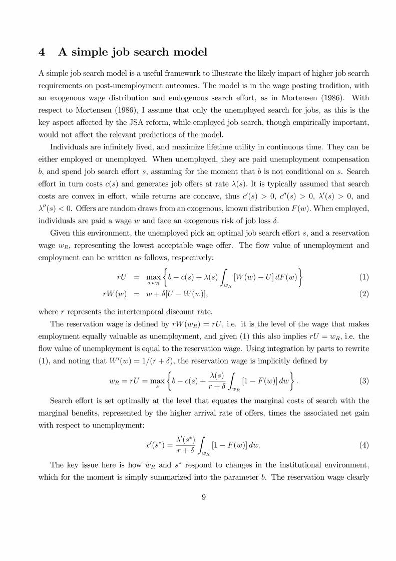
The JSA has been generally perceived as a major reform of the UK welfare system for the

unemployed, and some of its effects can be easily grasped by looking at time series of seasonally

adjusted flows in and out of registered unemployment, shown in Figure 1. Soon after JSA in-

troduction, there was a marked increase in the claimant outflow, with little or no impact on the

inflow into the claimant register. As Figure 2 shows, this translated into a more rapid decline in

the unemployment stock, which was already falling in the months preceding the reform. Indeed

official evaluations of the JSA carried by the then Department of Social Security (now Department

for Work and Pension) agree in documenting a very strong impact of the JSA on the flow off the

unemployment claimant register8. More recently, McVicar (2006) studies a case of excused signing

(and thus zero monitoring of search effort) within the JSA, during refurbishment of benefit offices

in Northern Ireland. He finds that periods with no monitoring strongly reduce the exit rate from

benefits. However, optimistic conclusions on job search and employment effects of search moni-

toring do not seem to be granted. Manning (2005) finds in fact that the JSA did not result in an

overall increase in job search effort, nor in higher job-finding rates. The next section illustrates

how these developments may in turn result in lower post-unemployment earnings and/or higher

labor force exits.8See for example Rayner et al. (2000) and Smith et al. (2000).

8

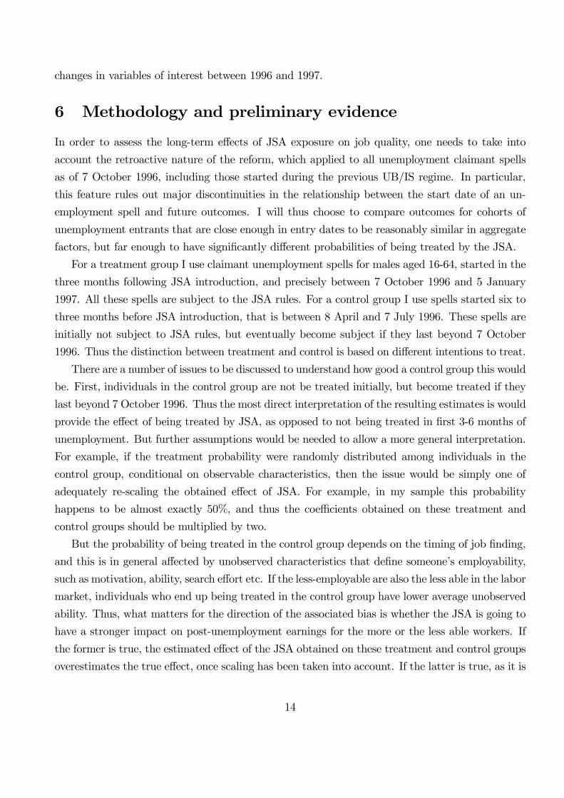
4 A simple job search model

A simple job search model is a useful framework to illustrate the likely impact of higher job search

requirements on post-unemployment outcomes. The model is in the wage posting tradition, with

an exogenous wage distribution and endogenous search effort, as in Mortensen (1986). With

respect to Mortensen (1986), I assume that only the unemployed search for jobs, as this is the

key aspect affected by the JSA reform, while employed job search, though empirically important,

would not affect the relevant predictions of the model.

Individuals are infinitely lived, and maximize lifetime utility in continuous time. They can be

either employed or unemployed. When unemployed, they are paid unemployment compensation

b, and spend job search effort s, assuming for the moment that b is not conditional on s. Search

effort in turn costs c(s) and generates job offers at rate λ(s). It is typically assumed that search

costs are convex in effort, while returns are concave, thus c0(s) > 0, c00(s) > 0, λ0(s) > 0, and

λ00(s) < 0. Offers are random draws from an exogenous, known distribution F (w).When employed,

individuals are paid a wage w and face an exogenous risk of job loss δ.

Given this environment, the unemployed pick an optimal job search effort s, and a reservation

wage wR, representing the lowest acceptable wage offer. The flow value of unemployment and

employment can be written as follows, respectively:

rU = maxs,wR

½b− c(s) + λ(s)

ZwR

[W (w)− U ] dF (w)

¾(1)

rW (w) = w + δ[U −W (w)], (2)

where r represents the intertemporal discount rate.

The reservation wage is defined by rW (wR) = rU , i.e. it is the level of the wage that makes

employment equally valuable as unemployment, and given (1) this also implies rU = wR, i.e. the

flow value of unemployment is equal to the reservation wage. Using integration by parts to rewrite

(1), and noting that W 0(w) = 1/(r + δ), the reservation wage is implicitly defined by

wR = rU = maxs

½b− c(s) +

λ(s)

r + δ

ZwR

[1− F (w)] dw

¾. (3)

Search effort is set optimally at the level that equates the marginal costs of search with the

marginal benefits, represented by the higher arrival rate of offers, times the associated net gain

with respect to unemployment:

c0(s∗) =λ0(s∗)

r + δ

ZwR

[1− F (w)] dw. (4)

The key issue here is how wR and s∗ respond to changes in the institutional environment,

which for the moment is simply summarized into the parameter b. The reservation wage clearly

9

increases with wR, as b directly affects unemployment income, which is forgone when one finds a

job. In particular:

dwR

db= r

dU

db= 1− λ(s)

r + δ[1− F (wR)]

dwR

db(5)

=r + δ

r + δ + λ(s) [1− F (wR)]> 0

A rise in b affects s∗ via its effect on wR, and in particular it lowers s∗ because by raising wR

it lowers the net returns to job search. Formally:

ds∗

db=

λ0(s∗)RwR[1− F (w)] dw

r + δ + λ(s∗) [1− F (wR)]

∙λ00(s∗)

r + δ

ZwR

[1− F (w)] dw − c00(s∗)

¸−1< 0.

The rate at which the unemployed find work is h = λ(s∗)[1 − F (wR)]. Thus a reduction in b

raises the job finding rate via both an increase in job search effort (and thus in the arrival rate of

offers) and a reduction in the reservation wage (and thus a fall in the rejection rate). At the same

time, it lowers the expected post-unemployment wage, E(w|w > wR).

Graphically, this can be seen by drawing indifference curves in the s, b space (as also done by

Manning, 2005). Utility while unemployed monotonically increases in b, while it increases in s for

s < s∗ and decreases in s for s > s∗:

rdU

ds=

r + δ

r + δ + λ(s) [1− F (wR)]

½λ0(s)

r + δ

ZwR

[1− F (w)] dw − c0(s)

¾. (6)

The indifference curves thus look like those represented in Figure 3, which also depicts the effect

of a fall in b. Higher curves are associated with higher levels of utility.

But as argued above, a change in the level of benefits was probably not the main feature of the

JSA, which instead mostly implied a change in search requirements for eligibility. Imagine now

that unemployment benefits are paid at the full rate for s equal to or higher than some threshold s,

and at some lower rate otherwise. The introduction of JSA implies an increase in such threshold.

Consider an individual who has indifference curves as those represented in Figure 4. The

increase in requirements from s1 to s2 would raise his optimal search effort from s∗1 to the corner

solution s∗2 = s2, and he would move on to a lower indifference curve, characterized by lower

utility and lower reservation wages. His job finding rate is thus higher, and these are precisely

the “intended” consequences of the JSA. Consider now an individual whose initial search effort

is lower, as illustrated in Figure 5, such that he barely meets the more lenient requirements, i.e.

s∗1 = s1. With the new requirements he would actually reduce his search effort. In other words,

not only would he not meet the new requirements s2, but also it would no longer be worthwhile

for him to keep his search effort as high as s1, thus s∗2 < s∗1. With lower reservation wages and

10

lower search effort, the effect of the increase in search requirements on the job finding rate of

the unemployed is ambiguous. These are “unintended” consequences of the JSA, emphasized by

Manning (2005) as one of factors why the JSA was not really successful at moving the unemployed

on to new jobs.

This framework delivers two main results that are going to be relevant for the empirical analysis

that follows. First, in any UI regime, workers with s∗ ≥ s are going to be formally classified as UI

claimants, while those with s∗ < s are non-claimants. Thus changes in s affect the composition of

the nonemployed between claimants and non-claimants. To see this, note that changes in s do not

affect optimal search intensity for workers with either very high initial search effort, i.e. s∗1 ≥ s2, or

very low initial search effort, i.e. s∗1 < s1. The former will be UI claimants in both regimes, while

the latter will always be non-claimants. But workers who pick initial search effort in the middle

range s1 ≤ s∗1 < s2 are affected by the change in search requirements. All of them are initially

claiming UI: some of them will find it optimal to search harder when s is raised (as in Figure 4),

and keep claiming UI; while others will reduce search effort (as in Figure 5), and stop claiming UI

in the new regime. This implies that an increase in s will raise the share of non-claimants among

the nonemployed population. They can be either non-claimant unemployed9 or nonparticipants,

and may or may not receive benefits that are not job search related.

Second, whether optimal search effort increases (Figure 4) or decreases (Figure 5), utility

enjoyed when unemployed unambiguously falls as a consequence of an increase in s, and this holds

even when the actual level of benefits received remains unchanged. This happens because some

cash payments that were initially made to the unemployed without too much questioning are now

made conditional on substantial search effort, with some associated costs. Thus one would expect

that an increase in s lowers reservation wages and the quality of post-unemployment jobs.

If on top of higher search requirements, the level of benefits is also falling, as it was the case

for workers aged 18-24 who were receiving UB before JSA introduction, this generates a stronger

fall in the reservation wage (as shown in Figure 3), and lowers the incentive to raise search effort

and meet the higher requirements, thus raising the proportion of workers who reduce search effort

as a consequence of JSA introduction. Thus any fall in the level of benefits would simply reinforce

the effects of tighter search requirements on both post-unemployment wages and outflows into

non-claimant unemployment.

9To fall in this category, a worker may not meet the JSA search requirements but meet instead the ILOunemployment definition, which classifies as unemployed those who have not worked more than one hour duringthe reference period but who are “available for and actively seeking work”.

11

5 Data

The data used in this paper are drawn from the Lifetime Labour Market Database (LLMDB),

administered by the Department for Work and Pensions. The LLMDB represents a 1% random

sample of social security records in Great Britain. Individuals covered are those whose National

Insurance numbers end in two given digits. The LLMDB provides a rich set of information on

labor histories of selected individuals from 1978 onwards. In particular, I will use information on

benefit spells and dependent labor income.

The LLMDB provides start and end dates of benefit spells, together with their type. Types

include job-search related benefits, like UB and IS in the old system and JSA in the new system;

health related benefits, like Incapacity Benefits (IB) or the Disability Living Allowance (DLA);

in-work benefits, like the Working Family Tax Credit (WFTC); retirement pensions; maternity

allowances; and a few others.

All information on benefit spells is in principle available since 1978, but the quality of benefit

spells data until 1995 is poorer than for the later period. For example, fewer benefit spells seem

to be recorded for the earlier period, and a relatively large proportion of them has missing end

dates, or imputed end dates.

I use unemployment claimants spells for 1996 and 1997. The LLMDB reports 45,982 unem-

ployment benefit spells started by British males between 1 January 1996 and 31 December 1997.

According to the UK Official Labour Market Statistics (Nomis), the male unemployment inflow

in the same period was 4,616,199. When LLMDB sampling is taken into account, the figures

stemming from the two sources are closely comparable.

Having said this, even in the post 1995 period, the accuracy of information on end dates of spells

is less accurate than that on start dates. In particular, the IS end dates have very strong quarterly

spikes. This happens because all relevant information about IS spells is collected quarterly by the

Department for Work and Pensions; thus if an individual features in the sample with an ongoing IS

spell at the start of a given quarter, but has disappeared from the sample at the end of the quarter,

he is assigned an imputed completion date corresponding to the middle date of the quarter. As

typically IS spells follow UB spells, this bunching problem is going to produce spikes in the end

dates of unemployment spells in my sample in the pre-JSA regime. For this reason I choose to

minimize the use of the end date of spells in my empirical analysis, and all selection criteria used

are based on spells start dates.

In the pre-JSA regime I construct unemployment spells by linking together UB and IS spells

that (partly) overlap, and UB and IS spells that do not overlap but have a maximum two weeks

window between the end date of the former and the start date of the latter. This is because a spell

12

out of benefits of less than two weeks is highly unlikely to represent a short job spell, and thus for

my purpose the corresponding benefit spells sequence best represents a single unemployment spell.

Also, and more importantly, bureaucratic procedures may require some time to move a claimant

from unemployment insurance to unemployment assistance benefits, and this may explain some

short gap between benefit spells. However, my estimation results were not sensitive to shortening

such window to 7 or zero days.

Information on employment and income is provided by fiscal years. Fiscal years in the UK

start on 6 April of a given year and end on 5 April of the following year, and in what follows all

annual indicators reported refer to fiscal, rather than calendar years. Employment and income

are represented by annual weeks worked and annual pre-tax pay, respectively. Both measures

are available from 1978 onwards. However, it should be noted that while from 1999 onwards the

number of weeks worked is reported directly within each National Insurance file, this has been

estimated by the Department for Work and Pensions for the period 1978-1998 using information on

known periods of nonemployment and self-employment. When applied to the post 1999 period, this

methodology reproduces fairly accurately the actual measure of weeks worked available (Needham,

2007).

Income data from the LLMDB have two main shortcomings. First, the LLMDB does not

currently contain employment spells dates, but it reports the number of employment spells recorded

in a given year, so that it is possible to know how many jobs someone has held in a given year,

with the associated weeks worked and pay, but it is not possible to know their start and end dates,

nor their chronological order. This implies that the best measure of wages from this survey is

average weekly wages over a fiscal year.

Second, the LLMDB does not provide information on weekly hours worked. This is mostly

a drawback for the analysis of female wages, given that the incidence of part-time work among

British women was fairly high (around 42% according to the Labour Force Survey) during my

period of observation. Thus I limit my analysis to British males.

Figure 6 display raw data on employment and earnings from the LLMDB between 1978 and

2003. The average number of weeks worked in a year declined steadily in the sample period,

while both annual and weekly earnings increased. Weekly earnings were increasing at an average

rate of 5.8% per year during the sample period, and this corresponds to an average 1.2% real

growth.10 It is worthwhile to notice the blip in annual weeks worked in 1997-1998 and the dip in

annual earnings in 1996. The apparent anomalies could be potentially explained by the fact that

recording methods changed in 1997, and the LLMDB was moved on to a new National Insurance

computerized system. The move from the old to the new system may in part explain the observed

10Using the retail price index from the Office for National Statistics.

13

changes in variables of interest between 1996 and 1997.

6 Methodology and preliminary evidence

In order to assess the long-term effects of JSA exposure on job quality, one needs to take into

account the retroactive nature of the reform, which applied to all unemployment claimant spells

as of 7 October 1996, including those started during the previous UB/IS regime. In particular,

this feature rules out major discontinuities in the relationship between the start date of an un-

employment spell and future outcomes. I will thus choose to compare outcomes for cohorts of

unemployment entrants that are close enough in entry dates to be reasonably similar in aggregate

factors, but far enough to have significantly different probabilities of being treated by the JSA.

For a treatment group I use claimant unemployment spells for males aged 16-64, started in the

three months following JSA introduction, and precisely between 7 October 1996 and 5 January

1997. All these spells are subject to the JSA rules. For a control group I use spells started six to

three months before JSA introduction, that is between 8 April and 7 July 1996. These spells are

initially not subject to JSA rules, but eventually become subject if they last beyond 7 October

1996. Thus the distinction between treatment and control is based on different intentions to treat.

There are a number of issues to be discussed to understand how good a control group this would

be. First, individuals in the control group are not be treated initially, but become treated if they

last beyond 7 October 1996. Thus the most direct interpretation of the resulting estimates is would

provide the effect of being treated by JSA, as opposed to not being treated in first 3-6 months of

unemployment. But further assumptions would be needed to allow a more general interpretation.

For example, if the treatment probability were randomly distributed among individuals in the

control group, conditional on observable characteristics, then the issue would be simply one of

adequately re-scaling the obtained effect of JSA. For example, in my sample this probability

happens to be almost exactly 50%, and thus the coefficients obtained on these treatment and

control groups should be multiplied by two.

But the probability of being treated in the control group depends on the timing of job finding,

and this is in general affected by unobserved characteristics that define someone’s employability,

such as motivation, ability, search effort etc. If the less-employable are also the less able in the labor

market, individuals who end up being treated in the control group have lower average unobserved

ability. Thus, what matters for the direction of the associated bias is whether the JSA is going to

have a stronger impact on post-unemployment earnings for the more or the less able workers. If

the former is true, the estimated effect of the JSA obtained on these treatment and control groups

overestimates the true effect, once scaling has been taken into account. If the latter is true, as it is

14

plausible, one obtains an underestimate of the true effect. My estimates control for detailed past

employment histories, which should act as a good proxy for a number of relevant unobservables

(see Card and Sullivan, 1988). As a robustness check, I will also perform a test solely based on

the short-term unemployed, so that the control group only contains spells that ended before JSA

introduction.

Second, I select control and treatment groups on the timing of job loss, and more precisely, on

the timing of signing-on for unemployment benefits. One may worry about strategic behavior in

the time of signing-on in the presence of anticipatory effects of JSA. And in principle individuals

may try to alter the signing-on behavior in the face of JSA by (i) signing-on earlier than they

would have done without the JSA; (ii) signing-on later; (iii) not signing-on at all. But how likely

is this kind of strategic behavior prior to JSA introduction? It may be argued that trying to

sign-on (shortly) earlier does not avoid treatment, as JSA is retroactive; signing-on later simply

implies loss of unemployment income, thus is clearly not optimal; and finally not signing-on at all

implies again loss of unemployment income: if one really dreads the prospect of the JSA interview

it is optimal to sign-on initially and then not show up for the first JSA interview.

Some indirect evidence on this can be grasped by looking at Figure 7, which gives the number of

claimant unemployment spells started between 1 January 1996 and 31 December 1997, and shows

no sign of any unusual behavior in the unemployment inflow around the time of JSA introduction.

Figure 8 provides a closer snapshot of the two months around JSA introduction. This reveals a

marked weekly pattern in starting dates, with Mondays being by far the busiest days, and the

frequency of new spells declining monotonically during the week, but again there is no evidence

of bunching of new spells shortly before or after 7 October.

It would be interesting to be able to observe the same kind of evidence in the unemployment

outflow, but as alrealy noted in Section 5 the LLMDB data are not ideal for this purpose, due

to heavily bunched ending dates of IS spells, which produce sizeable spikes in the end dates of

claimant unemployment spells, as shown in Figure 9. But official labor market data reported in

Figure 1 show no unusual behavior in the unemployment outflow just before JSA introduction,

with a strong fall immediately afterwards.

Finally, treatment and control groups are certainly going to be different as far as seasonal

factors are concerned. For this reason I construct treatment and control groups for the same

dates in 1997, and estimate the effect of JSA on future outcomes using a difference in differences

approach. I estimate an equation of the form

yi = β0 + β1C96i + β2Ti + β3

¡C96i ∗ Ti

¢+ γXi + εi (7)

where yi represents an outcome variable, Xi is a vector of individual characteristics, C96i is a

15

dummy variable for the 1996 cohort, Ti denotes treatment, and their interaction picks the effect

of JSA. Specification (7) is going to deliver an unbiased estimate for the coefficient of interest, β3,

if

E(εi|C96i = 0, Ti = 0, Xi)−E(εi|C96

i = 0, Ti = 1,Xi) =

E(εi|C97i = 0, Ti = 0, Xi)−E(εi|C97

i = 0, Ti = 1,Xi).

In other words, as treatment and control groups are selected on the basis of their date of job loss,

the underlying identifying assumption is that the correlation between the timing of job loss and

unobservables, if any, be the same across the two cohorts. This assumption is likely to be violated

if there are strong reasons to expect strategic signing-on timing, but I have argued above that this

is unlikely. Also, it would be worrying if control and treatment had markedly different observables

before JSA introduction, and this can be checked by looking at their employment and earnings

histories.

Descriptive statistics for treatment and control groups are reported in Table 1 and Figures

10-13. Table 1 reports information on age and the current unemployment spell. There are around

4,000 spells in each of the groups (treat and control in 1996 and 1997 cohorts). These groups are

very similar in their age, but differ in the duration of their current spell and in its destination. The

control group in the 1996 cohort tends to have longer spells than the three other groups, and this

is the main effect emphasized by the official evaluations of the JSA, although not with a difference

in differences approach. This group also has a lower probability to experience new benefit spells

in the near future.

More detailed information on annual earnings and weeks worked for the treatment and the

control groups is presented in Figures 10-13. Figure 10 gives the proportion of men with positive

earnings in each year for treatment and control groups in both the 1996 and 1997 cohorts. The

vertical line in correspondence of 1996 represents the introduction of JSA. This coincides with the

reference unemployment spell for the 1996 cohort, while the reference unemployment spell for the

1997 cohort takes place one year later. Overall, the fraction of men with positive earnings rises

for all groups by over 30 percentage points during the 10 years prior to JSA treatment, and this is

mostly an age effect, as the sample is relatively young. After treatment, the trend in such fraction

flattens out or even declines. It is also worthwhile to notice that the proportion with positive

earnings has a spike in the year of treatment, simply telling that the reference unemployment spell

tends to follow in most cases a period of paid employment.

Figure 11 reports the average number of annual weeks worked, conditional on working. In

this case the pre-shock trends are falling, and in particular individuals start experiencing negative

employment shocks around 6 years before the reference unemployment spell. After the JSA shock,

16

weeks worked increase, but it seems that part of the increase is due to the 1997-1998 blip in weeks

worked in the main database (see Figure 6). Figures 12 and 13 report log annual and weekly

earnings, respectively. Both measures of earnings decline sharply in the year of job loss, but

otherwise they follow a generally upward trend.

An interesting feature that stands out from Figures 10-13 is that pre-treatment trends are

in general very close for treatment and control groups in both cohorts. More importantly, the

associated difference in differences is never significantly different from zero for any of the variables

considered in the pre-treatment period. Figures 14-17 plot the difference in differences for the

same variables represented in Figures 10-13, where year 0 corresponds to 1996 for the 1996 cohort,

and to 1997 for the 1997 cohort. In Figure 14 a probit version of equation (7) is estimated; while

Figures 15-17 are based on OLS. The solid lines represent the point estimates (and, specifically,

marginal effects in Figure 14), and the dashed lines represent the 90% and 95% confidence intervals,

showing that, for the four labor market indicators considered, all point estimates lie within the

90% interval in the pre-treatment period. Recall that in order to consistently estimate β3 one

needs that any difference in unobservables between the treatment and control groups be the same

across the two cohorts. Using work histories as a proxy for individual unobservables, the evidence

presented in Figures 14-17 is in line with my identifying assumption.

It should finally be noted that some of the trends in Figures 10-13 seem to diverge after JSA

introduction, and in some cases more for the 1996 than the 1997 cohort, as also shown by point

estimates in Figures 14-17 for the post-treatment period. This is indicative of potential JSA effects

on future outcomes. The next section will provide more detailed results on these effects.

7 Results

7.1 Employment and earnings

I start by presenting evidence on the effects of JSA on the probability of leaving the unemployment

claimant register. Not only was this the main effect emphasized by the official evaluations of the

JSA, but also it could be the main channel through which one can expect more long-term effects.

I thus estimate a duration model of exit from unemployment, using a specification analogous

to (7), except that the duration model is non-linear. The results of the Cox proportional hazard

model are presented in the upper panel in Table 2, where the coefficients reported refer to the

interaction between the 1996 cohort and treatment, and thus are supposed to pick the effect of

JSA. All specifications also include separate dummy variables for treatment and the 1996 cohort.

The standard errors are clustered at the individual level, to cater for individuals with multiple

spells in this sample.

17

In the regression summarized in column 1, no other regressors are included, and the estimates

show a 10% increase in the unemployment exit hazard as a result of JSA. Column 2 also controls

for age, age squared, and past employment history (i.e. whether the individual had a claimant

unemployment spell in the previous two years, the total number of weeks worked and annual

earnings in each of the previous five years and their square).11 As expected from the evidence

presented in Table 1 and Figures 6-9, the inclusion of covariates hardly affects the results. The

next four columns show results for the young (aged 16-24) and the adult sample (aged 25-64)

separately. The JSA effect is still positive for both groups, but it is stronger for the adult sample,

while it does not reach the standard significance level for the young.

However, as information on ending dates of spells is heavily bunched at quarterly frequencies,

a continuous time duration model is probably not the best way to describe unemployment exit.

Another way to look at the effect of JSA on the outflow from the unemployment register consists

in comparing the fraction of the control group who are still claiming upon JSA introduction, i.e.

on 6 October 1996, with the fraction of the treatment group who, by symmetry, are still claiming

on 6 March 1997, as control and treatment groups are selected as entering unemployment six

months apart. This method has also the advantage of excluding a direct JSA effect on the exit

probability of the control group. The DID results from a probit model are presented in the lower

panel of Table 2, and show again a significant JSA effect on the probability to leave the register,

which is now higher for the young than the adult subsample.

Table 2 thus replicates the main result of the JSA evaluation literature, namely its strong

and significant impact on the exit rate from unemployment. But moving claimants off benefits

may not be equivalent to moving them on to new jobs. The LLMDB does not allow me to

fully characterize unemployment destinations, because it does not contain information on dates

of employment spells, but I can use information on weeks worked and earnings for the fiscal year

after treatment (and for later years) in order to assess the impact of JSA on both employment

and post-unemployment earnings.

Figures 18-21 present estimates of the effect of JSA on post-unemployment outcomes. Year 1

thus corresponds to 1997 for the 1996 cohort and to 1998 for the 1997 cohort. These estimates

are analogous to the post-treatment estimates presented in Figures 14-17, but unlike in Figures

14-17 they control for a number of observable characteristics, including the pre-treatment trends,

and also they distinguish between the young and the prime-age sample. Figure 18 shows the

effect of JSA on the probability of having positive earnings in the five years after the reference

unemployment spell for the whole sample and for the two age subgroups. JSA implied a reduction

of 4% in the probability of positive earnings in the year after the shock for the whole sample,

11Extending employment and earnings histories 10 instead of 5 years back produced virtually identical results.

18

and this effect is statistically significant at the 1% level. The JSA effect is roughly halved in the

second and third year (and it is only significant at the 10% level), and it finally tails off. For

those aged 16-24 the JSA effect is stronger to start with, and again is reabsorbed within the next

three years. For the prime age subsample the effect is weaker, and becomes non significantly

different from zero from the second year onwards. Registering for unemployment benefits soon

after JSA introduction, as opposed to six months earlier, implies thus a significant fall in the future

employment probability, and this effect is fairly long-lived especially for the youths.

Information on the actual number of weeks worked, conditional on having positive earnings,

is presented in Figures 19. The effect of JSA on weeks worked tends to be moderate and is

almost never significant for all age groups. Thus it seems that JSA mostly affected re-entry into

employment, without much of an effect on the number of weeks worked for those who did re-enter

employment.

Figure 20 present evidence on (log) annual earnings. Estimated effects are everywhere negative,

again stronger for the younger subsample, although they are often not significantly different from

zero. Figure 21 finally present estimates for weekly earnings, which are the variable most closely

related to post-unemployment job quality in this dataset. While the effect of JSA on weekly

earnings of the older subsample is quite close to zero and never significant throughout the post-

unemployment period, the corresponding effect for the younger sample is negative and significant

in years 2-4 after the shock. It is probably hard to reconcile such decline in weekly earnings with

the direct impact of JSA, because if anything one would expect an immediate effect in the first

year after the reference unemployment spell, which is gradually reabsorbed as individuals who are

initially mismatched search on-the-job for better matches. Some explanation of this behavior may

be related to the employment selection effects of JSA. Figure 18 has shown that the JSA had an

important initial impact on the proportion of individuals in work, which fades gradually over the

next five years, as the treated catch up with the non-treated in their employment levels. Thus the

employment stock may be of relatively high quality among the treated initially, because only the

most able have initially found work, and then quality declines as the less-able among the treated

find work. This selection mechanism may help explain why one does not find a JSA effect initially,

but finds instead a negative effect in the following years.

In summary, the most important effect of JSA on this sample is to reduce the probability to

have positive earnings after an unemployment shock, with more moderate and less precise effects

on the level of both annual and weekly earnings, and with almost no effect on the number of weeks

worked for those who re-enter employment. All effects tend to be stronger and more precisely

estimated for the younger sample. One explanation could be that for youths eligible for UB,

JSA introduction meant both an increase in search requirements, and a reduction in the benefit

19

level, with amplified effects on post-unemployment outcomes. But as argued in Section 3 this

explanation is unlikely, as the proportion of individuals eligible for UB only represents a minority

of observations. The other explanation is that the impact of search requirements alone may be

stronger for the youths, and this view seemed to be in line with the introduction of the New Deal

for Young People in April 1998, which combined JSA search requirements with intensive help with

job search (see Van Reenen, 2003).

7.2 Future benefit spells

Previous estimates show that the JSA raised the unemployment outflow, but at the same time also

raised the probability of not working at all in the following year, so one may wonder what happens

to individuals who leave the unemployment register but do not get jobs. One possibility is that

they may apply for and obtain other benefits, which are not conditional on active job search.

To answer this question I use information on different types of benefit spells contained in the

LLMDB. The UK welfare system, like most systems, includes several types of benefits, that can

be related to job search, income, health, work etc. For example, during the six months preceding

JSA introduction, between April and September 1996, the LLMDB registers about 77,000 benefit

spells. The most important category among these is represented by unemployment benefits, which

account for about three quarters of ongoing spells. The next category is represented by health-

related benefits, including Incapacity Benefits and the Disability Living Allowance. IB can be

claimed by individuals who are unable to work because of ill health or a disability, and accounts

for about 20% of benefit spells in the pre-JSA period. The DLA is a benefit for individuals who

need personal care due to mental or physical disabilities, and accounts for 10% of spells. Finally

come in-work benefits, represented by the Working Family Tax Credit, which includes just below

4% of benefit spells. One year later, that is between April and September 1997, there are about

63,000 benefit spells in the LLMDB. The importance of unemployment benefits has declined to

about 50%, and that of health-related benefits has increased to 24% for IB, and to 14% for DLA.

In-work benefits have also slightly risen to just over 5%.

To look at the impact of the JSA on unemployment exits into other benefits, I estimate a probit

version of equation (7), where the dependent variable is equal to 1 if an individual is receiving

benefits of any type within 1 month or within 6 months of the end of the reference unemploy-

ment spell, and zero otherwise. I then distinguish between new spells on IB, and new claimant

unemployment spells, whether on JSA, UB or IS. Destinations into other benefit categories are

not separately estimated because they represent a very small minority of my sample (see also

descriptive statistics presented in Table 1).

Table 3 reports results for a one-month window. When controlling for characteristics, individ-

20

uals treated by the JSA are on average 3.1% more likely to experience a new benefit spell within

one month of completing their current spell, and this effect is significant at the 5% level. Most of

the impact happens among the younger subsample, in which 4.5% of individuals experience new

benefit spells; while for the older subsample this figure falls to 2.4% and it is not significantly dif-

ferent from zero. The positive impact of JSA on exit into new benefit spells is explained in roughly

equal parts by spells on IB and new claimant unemployment spells, although the corresponding

effects only tend to be significant for new spells on IB.

Six months later the situation is more clear-cut, as shown in Table 4. Individuals affected are

3.4% more likely to be benefit recipients. The top panel of Figure 18 above has shown that the

JSA increases by 4.3% the probability of not working in the following year, and the estimates of

Table 4 tell that the bulk of such rise in nonemployment is explained by a higher take-up rate

of new benefits. The same observation holds looking at each age subsample separately. Among

new benefits, the biggest component is represented by IB. This last piece of evidence fits in the

increasing trend in take-up rates of IB in the UK and is consistent with the widespread view that

individuals who had lowest re-employment rates were actually advised by the Employment Service

to apply for IB (see Nickell and Quintini, 2002).

7.3 Robustness tests

The adopted definition of control and treatment groups, as well as some features of the data, require

a number of robustness checks. First, as noted in Figure 2, the unemployment inflow frequency

has a marked weekly pattern, and this may reflect the timing of initial benefit payments, rather

than the date a job loser initially approached the Employment Service. I thus converted the

benefit spells data from daily into weekly, by moving each start date to the previous and following

Mondays in turn, and constructed treatment and control groups in the same way as explained in

Section 6. The estimates obtained on this new sample were virtually identical to those obtained

on the original one.

Second, as treatment and control groups are selected according to their date of job loss for two

consecutive years, one may worry about interactions between seasonal factors and year effects. For

example, if the labor market were in general tighter in the fall (when the treatment is selected) than

in the spring (when the control is selected), and this effect were stronger in 1997 than in 1996, one

could potentially predict poorer lower relative re-employment prospects for the treatment group

in 1996 as a consequence of macroeconomic effects. Evidence on macroeconomic effects can be

provided by the monthly vacancy to unemployment ratio, which is typically used as a measure of

labor market tightness. This ratio increases roughly monotonically in Britain between January

1996 and December 1997, and thus shows no evidence of different seasonal patterns in 1996 and

21

1997. As a final check, I repeated the main estimates controlling for the value of labor market

tightness in the month of job loss, and the results stayed largely unchanged.

Fourth, I worked with a sample in which the control group has by definition a zero treatment

probability, by focusing on the short-term unemployed only. That is, I include in the control

group spells started between 8 April and 7 July 1996, and ended before 7 October 1996. None of

these can be treated by the JSA. For symmetry I include in the treatment group spells started

between 7 October 1996 and 5 January 1997, and ended before 7 April 1997, and then repeat

exactly the same procedure for entrants in spring and fall 1997. Of course it must be noted that

the short-term unemployed are a non-random sample of the unemployed population, and also

that the treatment effect needs not be the same across unemployment duration groups. But, in a

benchmark scenario in which the short-term unemployed are a random sample of the unemployed

(conditional on characteristics), and the JSA effect is homogeneous across duration groups (again,

conditional on characteristics), we would expect the estimated JSA effect on this sample to be

twice as large as the one obtained in the original sample, in which the control group in the 1996

cohort turns out to have a 50% treatment probability.

The results on post-unemployment work and earnings for the short-term unemployed are repre-

sented in Figures 22-25, where for simplicity only results on the two age subsamples are reported.

For example, Figure 22 shows that the JSA effect on the probability of positive earnings starts

off at about 20% for 16-24 year olds, and at about 6.5% for 25-64 year olds. The corresponding

effects for the main sample are 6.3% and 3.8% respectively (middle and bottom panel of Figure

18). Stronger JSA effects than on the main sample are also found in Figures 23-25. In particular,

the JSA impact on annual earnings is now initially significant for both age samples (Figure 24),

and the JSA impact on weekly earnings becomes significant for 25-64 year olds (Figure 25).

Table 5 represents the impact of JSA on exits into new benefit spells within either one or six

months from the completion of the current unemployment spell. Again all effects are stronger

than those reported in Table 3 and 4 for the main sample.

The final robustness test consists in a falsification check, based on treatment and control

groups for 1997 and 1998, constructed in the same way as I previously did for 1996 and 1997.

If my previous estimates identify the effect of JSA, one should obtain no significant effects of an

interaction term between the treatment and the 1997 cohort on this new sample, for any of the

post-unemployment outcomes considered. This is indeed what I obtain, as shown in Figures 26-29

for post-unemployment employment and earnings; and in Table 6 for exits into other benefit spells.

22

8 Conclusions

This paper has investigated the post-unemployment effects of higher job search requirements,

exploiting variation provided by the introduction of the UK JSA in October 1996. In a simple job

search framework, one expects that tighter requirements for UI eligibility lower the reservation

wage, with negative consequences on the quality of post-unemployment jobs, and raises the fraction

of non-claimant nonemployed.

Using administrative longitudinal data on spells on unemployment benefits and earnings, I find

that JSA has had a positive and significant impact on the claimant unemployment exit rate, as

well as on exits into other benefits, and a negative and significant impact on the probability of

working in the year after the unemployment spell. Starting a spell soon after JSA introduction, as

opposed to six months earlier, raises the likelihood of a spell on Incapacity Benefits by about 2.5-

3%, and lowers the likelihood of positive earnings by about 4%. At the same time, earnings for the

treated individuals seem to be lower than for the non treated after an unemployment shock, but

the confidence intervals around these estimated effects are quite large to exclude a wider variety

of scenarios. Overall, all the estimated effects tend to be stronger for the 16-24 than the 25-64

years old sample.

A possible interpretation is that tighter search requirements implied by the JSA indeed moved

claimants off unemployment benefits, without really raising job finding rates. Among claimants

treated by the JSA, those who found jobs quickly did not see their fortunes much changed with

respect to the previous regime, as implied by the absence of significant effects on weeks worked

and earnings in the year following job loss. But those who left the unemployment register without

finding a job were more likely to start spells on benefits that were not search related, and thus

to spend lower search effort and become more detached from the labor market than before the

JSA, with farily long-lasting effects on their employment rates. According to my estimates, the

JSA implied a net loss in (unconditional) weeks worked and earnings with respect to the previous

system during about three years after a job loss.

References

[1] Acemoglu, D. (2001), “Good Jobs versus Bad Jobs”, Journal of Labor Economics 19: 1-21.

[2] Acemoglu, D. and R. Shimer (1999), “Efficient Unemployment Insurance”,

Journal of Political Economy 107: 893-928.

[3] Acemoglu, D. and R. Shimer (2000), “Productivity Gains from Unemployment Insurance”,

European Economic Review 44: 1195-1224.

23

[4] Addison, J. and M. Blackburn (2000), “The Effects of Unemployment Insurance on Pos-

tunemployment Earnings”, Labour Economics 7: 21-53.

[5] Atkinson, A and J. Micklewright (1991), “Unemployment Compensation and Labor Market

Transitions: A Critical Review”, Journal of Economic Literature 29: 1679-1727.

[6] Ashenfelter, O., D. Ashmore and O. Deschenes (1999), “Do Unemployment Insurance Re-

cipients Actively Seek Work? Randomized Trials in Four US States”. NBER Working Paper

6982.

[7] Belzil, C. (2001), “Unemployment Insurance and Subsequent Job Duration: Job Matching

versus Unobserved Heterogeneity”. Journal of Applied Econometrics 16: 619-636.

[8] Burgess, P. and J. Kingston (1976), “The Impact of Unemployment Insurance Benefits on

Reemployment Success” Industrial and Labour Relations Review 30: 25-31.

[9] Card, D., R. Chetty and A. Weber (2007), “Cash-on-Hand and Competing

Models of Intertemporal Behavior: New Evidence from the Labor Market”.

Quarterly Journal of Economics, forthcoming.

[10] Card, D. and D. Sullivan (1988), “Measuring the Effect of Subsidized Training Programs on

Movements In and Out of Employment”. Econometrica 56: 497-530.

[11] Centeno, M. (2004), “The Match Quality Gains from Unemployment Insurance”,

Journal of Human Resources 39: 839-863.

[12] Classen, K. (1977), “The Effect of Unemployment Insurance on the Duration of Unemploy-

ment and Subsequent Earnings”. Industrial and Labour Relations Review 30: 438-50.

[13] Diamond, P. (1981), “Mobility Costs, Frictional Unemployment and Efficiency”,

Journal of Political Economy 89: 798-812.

[14] Dolton, P. and D. O’Neill (1996), “Unemployment Duration and the Restart Effect: Some

Experimental Evidence”, Economic Journal 106: 387-400.

[15] Dolton, P. and D. O’Neill (2002), “The Long-Run Effects of Unemployment Monitor-

ing and Work-Search Programs: Experimental Evidence from the United Kingdom”,

Journal of Labor Economics: 20, 381-403.

[16] Ehrenberg, R. and R. Oaxaca (1976), “Unemployment Insurance, Duration of Unemployment

and Subsequent Wage Gain”, American Economic Review 66: 754-766.

24

[17] Finn, D., I. Murray and C. Donnelly (1996), Unemployment and Training Rights Handbook,

London: The Unemployment Unit.

[18] Fredriksson and Holmlund (2006), “Improving Incentives in Unemployment Insurance”,

Journal of Economic Surveys 20: 357-386.

[19] Holen, A. (1977), “Effects of Unemployment Insurance Entitlement on Duration and Job

Search Outcome”. Industrial and Labor Relations Review 30: 445-450.

[20] Johnson, T. and D. Klepinger (1994), “Experimental Evidence on Unemployment Insurance

Work-Search Policies”, Journal of Human Resources 29: 695-717.

[21] Juraida, Š. (2002), “Estimating the Effect of Unemployment Insurance Compensation on the

Labor Market Histories of Displaced Workers”. Journal of Econometrics 108: 227-252.

[22] Lalive, R., J. van Ours and J. Zweimüller (2007), “How Changes in Financial Incentives Affect

the Duration of Unemployment ”, Review of Economic Studies 73: 1009-1038.

[23] Manning, A. (2005), “You Can’t Always Get What You Want: The Impact of the UK Job-

seekers’ Allowance”. CEP Discussion Paper 697.

[24] Marimon, R. and F. Zilibotti (1999), “Unemployment Vs. Mismatch of Talents: Reconsidering

Unemployment Benefits”, Economic Journal 109: 266-291.

[25] McVicar (2006), “Job Search Monitoring Intensity and Unemployment Exit: Evidence from

a Jobseeker’s Allowance Natural Experiment”, mimeo, Queen’s University Belfast.

[26] Meyer, B. (1995), “Lessons from the U.S. Unemployment Insurance Experiments”,

Journal of Economic Literature 33: 91-131

[27] Mortensen, D. (1986), “Job Search and Labor Market Analysis” in Ashenfelter, O. and R.

Layard (eds.) Handbook of Labor Economics, Volume 2, Amsterdam: North-Holland, pages

849-919.

[28] Needham, A. (2007), “Final Methodology for the Calculation of Class 1 Employee’s Weeks

Worked”. Mimeo, Department for Work and Pensions.

[29] Nickell, S. and G. Quintini (2002), “The Recent Performance of the UK Labour Market”,

Oxford Review of Economic Policy 18: 202-220.

25

[30] van Ours, J. and M. Vodopivec (2006), “Shortening the Potential Duration of Unemployment

Benefits Does Not Affect the Quality of Post-Unemployment Jobs: Evidence from a Natural

Experiment”. IZA Discussion Paper 2171.

[31] Paserman, D. (2007), “Job Search and Hyperbolic Dicounting: Structural Estimation and

Policy Evaluation”. Forthcoming in the Economic Journal.

[32] Pointer, R and M. Barnes (1997), Jobseeker’s Allowance Handbook, London: Child Poverty

Action Group.

[33] Rayner, E., S. Shah, R. White, L. Dawes and K. Tinsley (2000), “Evaluating Jobseeker’s

Allowance: A Summary of the Research Findings”, Department of Social Security, Research

Report No. 116.

[34] Smith, A., R. Youngs., K. Ashworth, S. McKay, R. Walker, with P. Elias and A. McKnight

(2000), “Understanding the Impact of Jobseeker’s Allowance”, Department of Social Security,

Research Report No. 111.

[35] Van Reenen, J. (2003) “Active Labour Market Policies and the British New Deal in Context”

NBER Working Paper 9576.

26

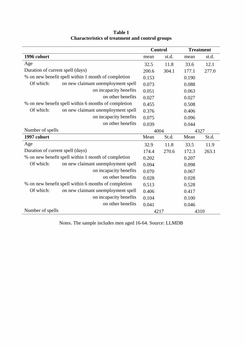
Table 1 Characteristics of treatment and control groups

Control Treatment 1996 cohort mean st.d. mean st.d. Age 32.5 11.8 33.6 12.1 Duration of current spell (days) 200.6 304.1 177.1 277.0 % on new benefit spell within 1 month of completion 0.153 0.190

Of which: on new claimant unemployment spell 0.073 0.088 on incapacity benefits 0.051 0.063

on other benefits 0.027 0.027 % on new benefit spell within 6 months of completion 0.455 0.508

Of which: on new claimant unemployment spell 0.376 0.406 on incapacity benefits 0.075 0.096

on other benefits 0.039 0.044 Number of spells 4004 4327 1997 cohort Mean St.d. Mean St.d. Age 32.9 11.8 33.5 11.9 Duration of current spell (days) 174.4 270.6 172.3 263.1 % on new benefit spell within 1 month of completion 0.202 0.207

Of which: on new claimant unemployment spell 0.094 0.098 on incapacity benefits 0.070 0.067

on other benefits 0.028 0.028 % on new benefit spell within 6 months of completion 0.513 0.528

Of which: on new claimant unemployment spell 0.406 0.417 on incapacity benefits 0.104 0.100

on other benefits 0.041 0.046 Number of spells 4217 4310

Notes. The sample includes men aged 16-64. Source: LLMDB

Table 2 Impact of JSA on claimant outflow

Cox proportional hazard model Ages 16-64 Ages 16-24 Ages 25-64 JSA 0.099*** 0.106*** 0.063 0.083 0.104*** 0.108*** [s.e] [0.031] [0.031] [0.055] [0.054] [0.038] [0.038] Observations 16423 16423 5320 5320 11103 11103 Other controls No Yes No Yes No Yes Whether still claiming at the end of the semester Ages 16-64 Ages 16-24 Ages 25-64 JSA -0.149*** -0.154*** -0.180*** -0.190*** -0.127*** -0.130*** [s.e] [0.014] [0.014] [0.023] [0.023] [0.017] [0.017] Observations 16858 16858 5499 5499 11359 11359 Other controls No Yes No Yes No Yes Notes. Estimation methods: Cox proportional hazard model in the upper panel and probit model in the lower panel (marginal effects reported). JSA=C96*Treat, and regressions also control for treatment and C96separately. Other controls included are: age, age squared, whether had an unemployment spell in the previous 2 years, total weeks worked in each of the past 5 years and their square, total earnings in each of the past 5 years and their square. Standard errors are clustered at the individual level and reported in brackets.

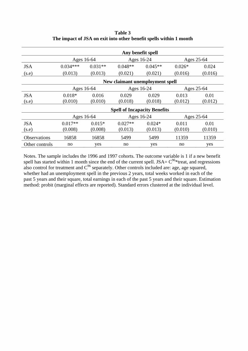
Table 3 The impact of JSA on exit into other benefit spells within 1 month

Any benefit spell Ages 16-64 Ages 16-24 Ages 25-64 JSA 0.034*** 0.031** 0.048** 0.045** 0.026* 0.024 (s.e) (0.013) (0.013) (0.021) (0.021) (0.016) (0.016)

New claimant unemployment spell Ages 16-64 Ages 16-24 Ages 25-64 JSA 0.018* 0.016 0.029 0.029 0.013 0.01 (s.e) (0.010) (0.010) (0.018) (0.018) (0.012) (0.012)

Spell of Incapacity Benefits Ages 16-64 Ages 16-24 Ages 25-64 JSA 0.017** 0.015* 0.027** 0.024* 0.011 0.01 (s.e) (0.008) (0.008) (0.013) (0.013) (0.010) (0.010)

Observations 16858 16858 5499 5499 11359 11359 Other controls no yes no yes no yes Notes. The sample includes the 1996 and 1997 cohorts. The outcome variable is 1 if a new benefit spell has started within 1 month since the end of the current spell. JSA= C96*treat, and regressions also control for treatment and C96 separately. Other controls included are: age, age squared, whether had an unemployment spell in the previous 2 years, total weeks worked in each of the past 5 years and their square, total earnings in each of the past 5 years and their square. Estimation method: probit (marginal effects are reported). Standard errors clustered at the individual level.

Table 4 The impact of JSA on exit into other benefit spells within 6 months

Age sample 16-64 16-24 25-64 16-64 16-24 25-64

Any benefit spell JSA 0.038** 0.034** 0.045* 0.037 0.034* 0.029 (s.e) (0.015) (0.015) (0.026) (0.027) (0.019) (0.019)

New claimant unemployment spell JSA 0.020 0.017 0.037 0.031 0.013 0.007 (s.e) (0.015) (0.015) (0.027) (0.027) (0.018) (0.018)

Spell of Incapacity Benefits JSA 0.027*** 0.024** 0.030** 0.026* 0.025** 0.022* (s.e) (0.010) (0.010) (0.015) (0.015) (0.013) (0.012)

Observations 16858 16858 5499 5499 11359 11359 Other controls no yes no yes no yes Notes. The sample includes the 1996 and 1997 cohorts. The outcome variable is 1 if a new benefit spell has started within 6 months since the end of the current spell. JSA= C96*treat, and regressions also control for treatment and C96 separately. Other controls included are: age, age squared, whether had an unemployment spell in the previous 2 years, total weeks worked in each of the past 5 years and their square, total earnings in each of the past 5 years and their square. Estimation method: probit (marginal effects are reported). Standard errors clustered at the individual level

Table 5 The impact of JSA on exit into other benefit spells within 1 month

Short-term unemployed only

Any benefit spell

Within 1 month Within 6 months Ages 16-24 Ages 25-64 Ages 16-64 Ages 25-64 JSA 0.078*** 0.056*** 0.041 0.038 (s.e) (0.029) (0.020) (0.035) (0.024)

New claimant unemployment spell

Within 1 month Within 6 months Ages 16-64 Ages 25-64 Ages 16-64 Ages 25-64 JSA 0.030 0.019 0.004 0.021 (s.e) (0.023) (0.015) (0.035) (0.024)

Spell of Incapacity benefits

Within 1 month Within 6 months Ages 16-64 Ages 25-64 Ages 16-64 Ages 25-64 JSA 0.048** 0.031** 0.065*** 0.030** (s.e) (0.019) (0.013) (0.024) (0.015)

Observations 3453 6762 3453 6762 Other controls yes yes yes yes

Notes. The sample includes the short-term unemployed from 1996 and 1997 cohorts. Short-term unemployed are defined as those who exit unemployment by the beginning of October (respectively April) if in the treatment (respectively control) group. The outcome variable is 1 if a new benefit spell has started within 1 or 6 month since the end of the current spell. JSA= C96*treat, and regressions also control for treatment and C96 separately. Other controls included are: age, age squared, whether had an unemployment spell in the previous 2 years, total weeks worked in each of the past 5 years and their square, total earnings in each of the past 5 years and their square. Estimation method: probit (marginal effects are reported). Standard errors clustered at the individual level.

Table 6 The impact of JSA on exit into other benefit spells

Falsification test on 1997 and 1998 cohorts

Any benefit spell

Within 1 month Within 6 months Ages 16-24 Ages 25-64 Ages 16-64 Ages 25-64 JSA 0.030 -0.009 -0.037 -0.008 (s.e) (0.021) (0.015) (0.027) (0.019)

New claimant unemployment spell

Within 1 month Within 6 months Ages 16-64 Ages 25-64 Ages 16-64 Ages 25-64 JSA 0.013 -0.008 -0.040 -0.009 (s.e) (0.017) (0.011) (0.027) (0.018)

Spell of Incapacity benefits

Within 1 month Within 6 months Ages 16-64 Ages 25-64 Ages 16-64 Ages 25-64 JSA 0.012 0.001 0.004 0.001 (s.e) (0.012) (0.010) (0.014) (0.012)

Observations 5366 11303 5366 11303 Other controls yes yes yes yes

Notes. The sample includes the 1997 and 1998 cohorts. The outcome variable is 1 if a new benefit spell has started within 1 or 6 month since the end of the current spell. JSA= C97*treat, and regressions also control for treatment and C97 separately. Other controls included are: age, age squared, whether had an unemployment spell in the previous 2 years, total weeks worked in each of the past 5 years and their square, total earnings in each of the past 5 years and their square. Estimation method: probit (marginal effects are reported). Standard errors clustered at the individual level.

Figure 1: Flows out of and into the claimant unemployment register

Data seasonally adjusted. Source: NOMIS

Figure 2: The claimant unemployment count

Data seasonally adjusted. Source: NOMIS

200

250

300

350

400

thou

sand

s

1990 1995 2000 2005year

outflow inflow

1000

1500

2000

2500

3000

thou

sand

s

1990 1995 2000 2005year

Figure 3 Indifference curves between benefit levels and search effort

s

b

s1* s2

*

b2

b1

rU1=wR1

rU2=wR2

Figure 4 Intended consequences of tighter eligibility requirements

Figure 5 Unintended consequences of tighter eligibility requirements

s

b

s1*= s1 s2

*

rU2=wR2

rU1=wR1

s2

s

b

s2*= s2 s1

*

rU2=wR2

rU1=wR1

s1

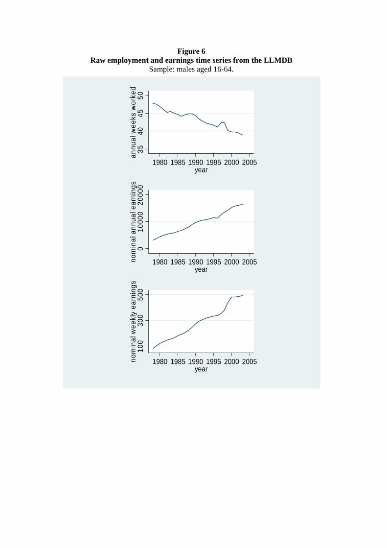
Figure 6 Raw employment and earnings time series from the LLMDB

Sample: males aged 16-64.

3540

4550

annu

al w

eeks

wor

ked

1980 1985 1990 1995 2000 2005year

010

000

2000

0no

min

al a

nnua

l ear

ning

s

1980 1985 1990 1995 2000 2005year

100

300

500

nom

inal

wee

kly

earn

ings

1980 1985 1990 1995 2000 2005year

Figure 7 Claimant unemployment spells started 1 Jan n1996-31 Dec 1998

Source: LLMDB

Figure 8 Claimant unemployment spells started 1 Sept -31 Oct 1996

Source: LLMDB

JSA introduction

050

100

150

200

250

No.

Spe

lls s

tarte

d

01jan1996 01jul1996 01jan1997 01jul1997 01jan1998Date

JSA introduction

050

100

150

No.

Spe

lls s

tarte

d

01sep1996 01oct1996 01nov1996Date

Figure 9 Claimant unemployment spells ended 1 Jan 1996-31 Dec 1998

Source: LLMDB

050

010

0015

0020

00N

o. s

pells

end

ed

01jan1996 01jul1996 01jan1997 01jul1997 01jan1998date

Figure 10 The proportion of individuals with positive earnings in control and treatment groups

Sample: Males 16-64. Source: LLMDB

Figure 11 Average number of weeks worked among the employed in control and treatment groups

Sample: Males 16-64. Source: LLMDB

3035

4045

1985 1990 1995 2000 20051985 1990 1995 2000 2005

1996 cohort 1997 cohort

control treat

annu

al w

eeks

wor

ked

| wee

ks>0

year

Graphs by cohortw

.4.5

.6.7

.8

1985 1990 1995 2000 20051985 1990 1995 2000 2005

1996 cohort 1997 cohort

control treat

prop

ortio

n w

ith p

ositi

ve a

nnua

l ear

ning

s

year

Graphs by cohortw

Figure 12 Log annual earnings in control and treatment groups

Sample: Males 16-64. Source: LLMDB

Figure 13 Log weekly earnings in control and treatment groups

Sample: Males 16-64. Source: LLMDB

4.5

55.

56

1985 1990 1995 2000 20051985 1990 1995 2000 2005

1996 cohort 1997 cohort

control treat

log

wee

kly

earn

ings

year

Graphs by cohortw

88.

59

9.5

1985 1990 1995 2000 20051985 1990 1995 2000 2005

1996 cohort 1997 cohort

control treat

log

annu

al e

arni

ngs

year

Graphs by cohortw

Figure 14 DID estimates of the probability to have positive earnings

Figure 15 DID estimates of the number of weeks worked among the employed

-2-1

01

2

-12 -10 -8 -6 -4 -2 0 2 4 6years from shock

-.08

-.06

-.04

-.02

0.0

2.0

4

-12 -10 -8 -6 -4 -2 0 2 4 6years from shock

Figure 16 DID estimates of log annual earnings

Figure 17 DID estimates of log weekly earnings

-.1-.0

50

.05

.1

-12 -10 -8 -6 -4 -2 0 2 4 6years from shock

Notes to Figures 14-17. The solid line represents marginal effects (Figure 14) or coefficients (Figures 15-17) on the C96*Treat interaction (see equation (7)), and regressions also control for treatment and C96 separately. The dashed lines represent 90% and 95% confidence intervals. Time zero denotes 1996 for the 1996 cohort; and 1997 for the 1997 cohort. Sample: Males 16-64. Source: LLMDB.

-.2-.1

0.1

.2

-12 -10 -8 -6 -4 -2 0 2 4 6years from shock

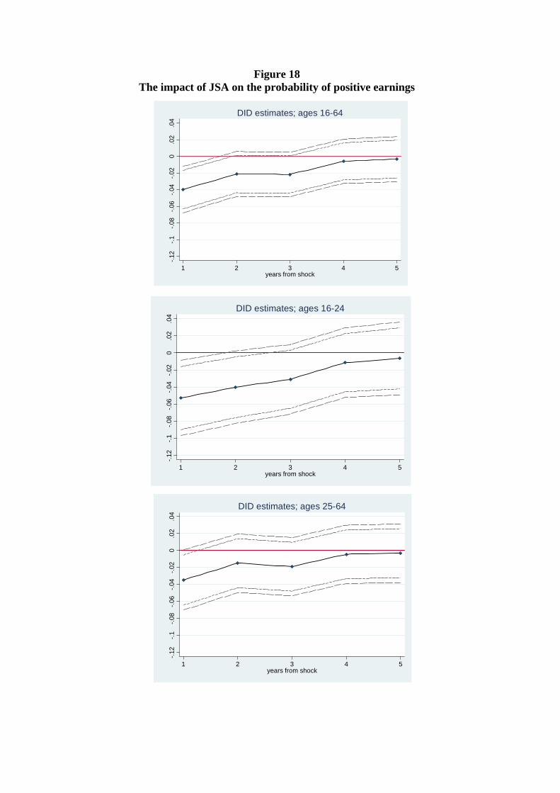
Figure 18 The impact of JSA on the probability of positive earnings

.02

.04

0-.0

2-.0

4-.0

6-.0

8-.1

-.12

1 2 3 4 5years from shock

DID estimates; ages 16-64

.02

.04

0-.0

2-.0

4-.0

6-.0

8-.1

-.12

1 2 3 4 5years from shock

DID estimates; ages 16-24

.02

.04

0-.0

2-.0

4-.0

6-.0

8-.1

-.12

1 2 3 4 5years from shock

DID estimates; ages 25-64

Figure 19 The impact of JSA on the number of weeks worked among the employed

-4-3

-2-1

01

23

1 2 3 4 5years from shock

DID estimates; ages 16-64

-4-3

-2-1

01

23

1 2 3 4 5years from shock

DID estimates; ages 16-24

-4-3

-2-1

01

23

1 2 3 4 5years from shock

DID estimates; ages 25-64

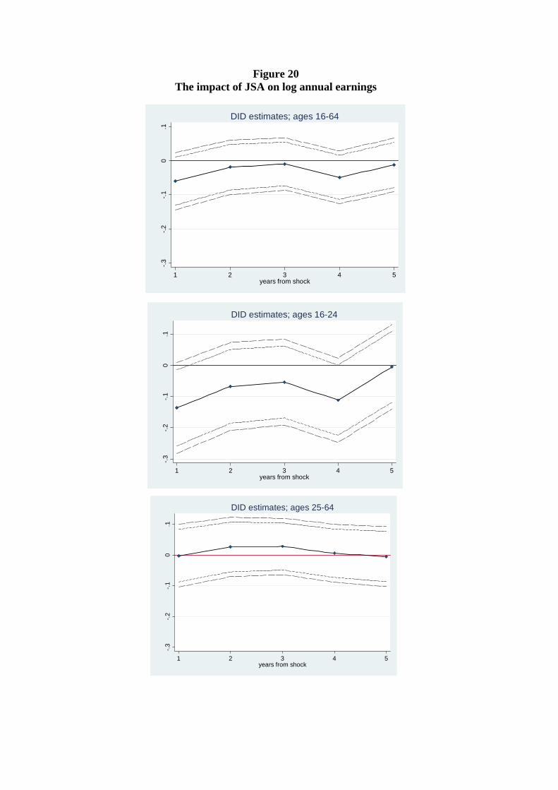
Figure 20 The impact of JSA on log annual earnings

-.3-.2

-.10

.1

1 2 3 4 5years from shock

DID estimates; ages 16-64

-.3-.2

-.10

.1

1 2 3 4 5years from shock

DID estimates; ages 16-24

-.3-.2

-.10

.1

1 2 3 4 5years from shock

DID estimates; ages 25-64

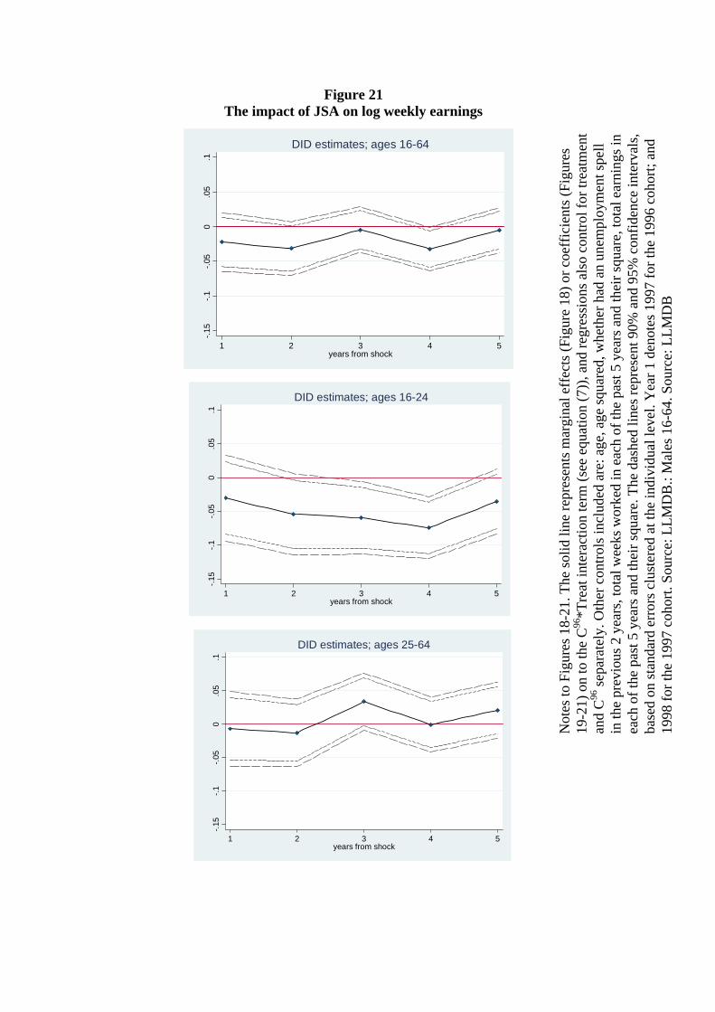
Figure 21 The impact of JSA on log weekly earnings

Not

es to

Fig

ures

18-

21. T

he so

lid li

ne re

pres

ents

mar

gina

l eff

ects

(Fig

ure

18) o

r coe

ffic

ient

s (Fi

gure

s 19

-21)

on

to th

e C

96*T

reat

inte

ract

ion

term

(see

equ

atio

n (7

)), a

nd re

gres

sion

s als

o co

ntro

l for

trea

tmen

t an

d C

96 se

para

tely

. Oth

er c

ontro

ls in

clud

ed a

re: a

ge, a

ge sq

uare

d, w

heth

er h

ad a

n un

empl

oym

ent s

pell

in th

e pr

evio

us 2

yea

rs, t

otal

wee

ks w

orke

d in

eac

h of

the

past

5 y

ears

and

thei

r squ

are,

tota

l ear

ning

s in

each

of t

he p

ast 5

yea

rs a

nd th

eir s

quar

e. T

he d

ashe

d lin

es re

pres

ent 9

0% a

nd 9

5% c

onfid

ence

inte

rval

s, ba

sed

on st

anda

rd e

rror

s clu

ster

ed a

t the

indi

vidu

al le

vel.

Yea

r 1 d

enot

es 1

997

for t

he 1

996

coho

rt; a

nd

1998

for t

he 1

997

coho

rt. S

ourc

e: L

LMD

B.:

Mal

es 1

6-64

. Sou

rce:

LLM

DB

-.15

-.1-.0

50

.05

.1

1 2 3 4 5years from shock

DID estimates; ages 16-64

-.15

-.1-.0

50

.05

.1

1 2 3 4 5years from shock

DID estimates; ages 16-24

-.15

-.1-.0

50

.05

.1

1 2 3 4 5years from shock

DID estimates; ages 25-64

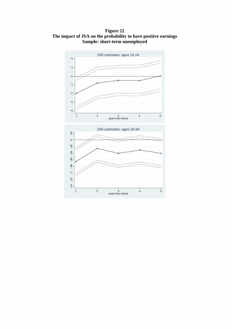
Figure 22 The impact of JSA on the probability to have positive earnings

Sample: short-term unemployed

.02

0-.0

2-.0

4-.0

6-.0

8-.1

-.12

-.14

1 2 3 4 5years from shock

DID estimates; ages 25-64

-.4-.3

-.2-.1

0.1

.2

1 2 3 4 5years from shock

DID estimates; ages 16-24

Figure 23 The impact of JSA on the number of weeks worked among the employed

Sample: short-term unemployed

-4-3

-2-1

01

23

4

1 2 3 4 5years from shock

DID estimates; ages 25-64

-4-3

-2-1

01

23

4

1 2 3 4 5years from shock

DID estimates; ages 16-24

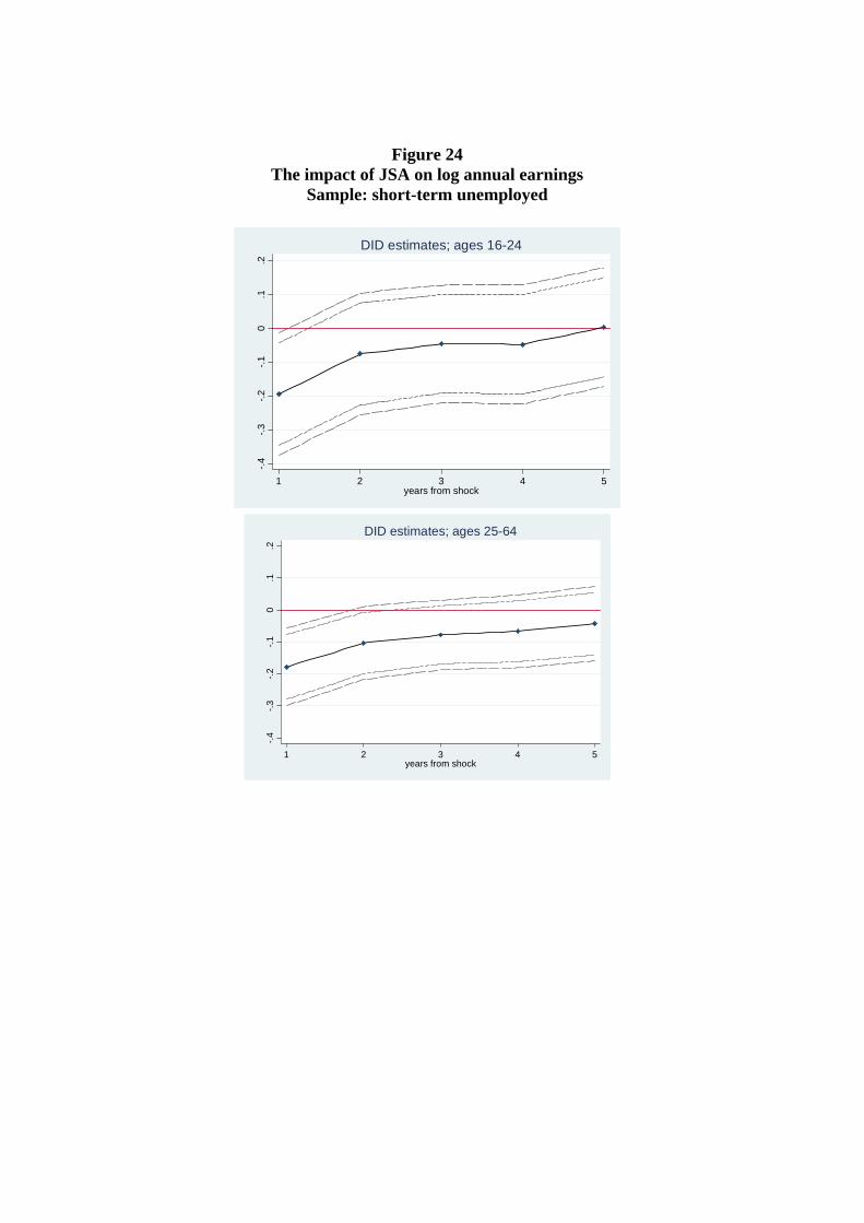
Figure 24 The impact of JSA on log annual earnings

Sample: short-term unemployed

-.4-.3

-.2-.1

0.1

.2

1 2 3 4 5years from shock

DID estimates; ages 25-64

-.4-.3

-.2-.1

0.1

.2

1 2 3 4 5years from shock

DID estimates; ages 16-24

Figure 25 The impact of JSA on log weekly earnings

Sample: short-term unemployed

Notes to Figures 22-25. The sample includes the short-term unemployed from 1996 and 1997 cohorts. Short-term unemployed are defined as those who exit unemployment by the beginning of October (respectively April) if in the treatment (respectively control) group. The solid line represents marginal effects (Figure 22) or coefficients (Figures 23-25) on to the C96*Treat interaction term (see equation (7)), and regressions also control for treatment and C96 separately. Other controls included are: age, age squared, whether had an unemployment spell in the previous 2 years, total weeks worked in each of the past 5 years and their square, total earnings in each of the past 5 years and their square. The dashed lines represent 90% and 95% confidence intervals, based on standard errors clustered at the individual level. Year 1 denotes 1997 for the 1996 cohort; and 1998 for the 1997 cohort. Source: LLMDB.

-.2-.1

5-.1

-.05

0.0

5

1 2 3 4 5years from shock

DID estimates; ages 25-64

-.15

-.1-.0

50

.05

1 2 3 4 5years from shock

DID estimates; ages 16-24

Figure 26 The impact of JSA on the probability to have positive earnings

Falsification test on 1997 and 1998 cohorts

.06

.02

.04

0-.0

2-.0

4-.0

6

1 2 3 4 5years from shock

DID estimates; ages 16-24.0

6.0

2.0

40

-.02

-.04

-.06

1 2 3 4 5years from shock

DID estimates; ages 25-64

Figure 27 The impact of JSA on weeks worked for the employed

Falsification test on 1997 and 1998 cohorts

-4-3

-2-1

01

23

4

1 2 3 4 5years from shock

DID estimates; ages 16-24

-4-3

-2-1

01

23

4

1 2 3 4 5years from shock

DID estimates; ages 25-64

Figure 28 The impact of JSA on log annual earnings Falsification test on 1997 and 1998 cohorts

.2.1

0-.2

-.1

1 2 3 4 5years from shock

DID estimates; ages 16-24.2

.10

-.2-.1

1 2 3 4 5years from shock

DID estimates; ages 25-64

Figure 29 The impact of JSA on log weekly earnings Falsification test on 1997 and 1998 cohorts

Notes to Figures 26-29. The sample includes the 1997 and 1998 cohorts. The solid line represents marginal effects (Figure 26) or coefficients (Figures 27-29) on to the C97*Treat interaction term (see equation (7)), and regressions also control for treatment and C97 separately. Other controls included are: age, age squared, whether had an unemployment spell in the previous 2 years, total weeks worked in each of the past 5 years and their square, total earnings in each of the past 5 years and their square. The dashed lines represent 90% and 95% confidence intervals, based on standard errors clustered at the individual level. Year 1 denotes 1998 for the 1997 cohort; and 1999 for the 1998 cohort. Source: LLMDB.

.1.0

50

-.05

-.1

1 2 3 4 5years from shock

DID estimates; ages 16-24.1

.05

0-.0

5-.1

1 2 3 4 5years from shock

DID estimates; ages 25-64

CENTRE FOR ECONOMIC PERFORMANCE Recent Discussion Papers

840 Kevin D. Sheedy Robustly Optimal Monetary Policy

839 Christopher A. Pissarides The Unemployment Volatility Puzzle: Is Wage Stickiness the Answer?

838 Kevin D. Sheedy Inflation Persistence when Price Stickiness Differs between Industries

837 Kevin D. Sheedy Intrinsic Inflation Persistence

836 Andrew E. Clark Ed Diener Yannis Georgellis Richard E. Lucas

Lags and Leads in Life Satisfaction: A Test of the Baseline Hypothesis

835 Jean-Baptiste Michau Creative Destruction with On-the-Job Search

834 Nikolaus Wolf Scylla and Charybodis: the European Economy and Poland's Adherence to Gold, 1928-1936

833 Sharon Belenzon Tomer Berkovitz

Innovation in Business Groups

832 Espen R. Moen Åsa Rosén

Incentives in Competitive Search Equilibrium

831 Eran Yashiv U.S. Labor Market Dynamics Revisited

830 Laura Alfaro Andrew Charlton

Growth and the Quality of Foreign Direct Investment: Is All FDI Equal?

829 Richard Layard David Clark Martin Knapp Guy Mayraz

Cost-Benefit Analysis of Psychological Therapy

828 Emma Tominey Maternal Smoking During Pregnancy and Early Child Outcomes

827 Christos Genakos Tommaso Valletti

Testing the “Waterbed” Effect in Mobile Telephony

826 Luis Garicano Paul Heaton

Information Technology, Organization, and Productivity in the Public Sector: Evidence from Police Departments

825 Laura Alfaro Andrew Charlton

Intra-Industry Foreign Direct Investment

824 Miklós Koren Silvana Tenreyro

Technological Diversification

823 Régis Barnichon The Shimer Puzzle and the Correct Identification of Productivity Shocks

822 Carlos Thomas Search Frictions, Real Rigidities and Inflation Dynamics

821 Giulia Faggio Kjell G. Salvanes John Van Reenen

The Evolution of Inequality in Productivity and Wages: Panel Data Evidence

820 Luis Araujo Emanuel Ornelas

Trust-Based Trade

819 Régis Barnichon Productivity, Aggregate Demand and Unemployment Fluctuations

818 Rachel Griffith Sokbae Lee John Van Reenen

Is Distance Dying at Last? Falling Home Bias in Fixed Effects Models of Patent Citations

817 Tsutomu Miyagawa YoungGak Kim

Measuring Organization Capital in Japan: An Empirical Assessment Using Firm-Level Data

816 Andreas Georgiadis Alan Manning

Spend It Like Beckham? Inequality and Redistribution in the UK, 1983-2004

815 Guy Michaels Xiaojia Zhi

Freedom Fries

814 Ralph Ossa Trade Liberalization, Outsourcing, and Firm Productivity

813 Karsten Kohn Alexander C. Lembcke

Wage Distributions by Bargaining Regime: Linked Employer-Employee Data Evidence from Germany

812 Yannis M. Ioannides Henry G. Overman Esteban Rossi-Hansberg Kurt Schmidheiny

The Effect of Information and Communication Technologies on Urban Structure

811 Guy Michaels The Division of Labor, Coordination, and the Demand for Information Processing

810 Maia Güell Jose V. Rodriguez Mora Chris Telmer

Intergenerational Mobility and the Informative Content of Surnames

The Centre for Economic Performance Publications Unit Tel 020 7955 7673 Fax 020 7955 7595 Email info@cep.lse.ac.uk

Web site http://cep.lse.ac.uk