Centrum voor Wiskunde en Informatica

REPORTRAPPORT

Computer Assisted Manipulation of Algebraic Process Specifications

J.F. Groote, B. Lisser

Software Engineering (SEN)

SEN-R0117 May 31, 2001

Report SEN-R0117ISSN 1386-369X

CWIP.O. Box 940791090 GB AmsterdamThe Netherlands

CWI is the National Research Institute for Mathematicsand Computer Science. CWI is part of the StichtingMathematisch Centrum (SMC), the Dutch foundationfor promotion of mathematics and computer scienceand their applications.SMC is sponsored by the Netherlands Organization forScientific Research (NWO). CWI is a member ofERCIM, the European Research Consortium forInformatics and Mathematics.

Copyright © Stichting Mathematisch CentrumP.O. Box 94079, 1090 GB Amsterdam (NL)

Kruislaan 413, 1098 SJ Amsterdam (NL)Telephone +31 20 592 9333

Telefax +31 20 592 4199

Computer Assisted Manipulation of Algebraic Process Specifications

Jan Friso Groote and Bert LisserJ.F.Groote@tue.nl, Bert.Lisser@cwi.nl

CWI

P.O. Box 94079, 1090 GB Amsterdam, The Netherlands

ABSTRACT

Specifications of system behaviour tend to become large. Analysis of such specifications requires automated

tools. Most attention hitherto has been invested in fully automatic tools. We however believe that in many

cases human intervention is required and we therefore propose a number of computer tools to transform

process specifications. The concrete manipulation tools that we describe can eliminate constants, redundant

sum variables and parameters, and allow to split variables ranging over complex datatypes. These tools can

transform specifications with large finite state spaces to variants with state spaces being a fraction of their

original size, and transform specifications with infinite state spaces to those with finite state spaces.

2000 Mathematics Subject Classification: 68M14, 68Q60, 68Q85

Keywords and Phrases: Automated Reasoning, Distributed systems, Linear Process Equations, Model Checking,

Verification

Note: Research carried out in SEN2, with financial support of the ”Systems Validation Center”.

1. Introduction

Tools and techniques for the analysis of system behaviour become increasingly powerful. Currently,we can regularly, automatically and thus efficiently answer questions about systems with a restrictedstate space, and we can also occasionally obtain insight in the behaviour of more substantial systems.But the results in this last category, often require ingenuity, insight in the problem domain, and oftenthe ad hoc design or adaption of tools.

We believe that this is typical for the study of more complex systems. In the first place, fullyautomatic analysis tools are generally not able to perform the analysis of complex systems fully ontheir own. This explains why human ingenuity is required in the process. In the second place, it isout of the question that these systems be analysed by hand only. The size of such descriptions mayliterally stretch to up to thousands of pages. This is why automation is needed.

We think that it is not desired that for each complex system to be analysed in the future, newtransformation programs must be designed, or old analysis programs must be adapted. It is better toprovide a set of manipulation tools that can be used to preprocess and transform a given system suchthat it fits a standard analysis tool.

Note that such a situation is not very uncommon in the field of mathematical analysis. Typicalmathematical analysis tools such as Mathematica and Maple do not attempt to solve a formula ontheir own, but they operate under strict supervision of a user, who, when sufficiently skilled in theuse of such a tool, can lead the system to an answer.

In this paper we describe a number of transformation tools that we have developed. We show howin certain cases we can manipulate descriptions of distributed systems to reduce their state spacesfrom infinite to finite, or to a fraction of their original size.

We work in the setting of process algebra with data µCRL [10], or more precisely in the setting oflinear process equations. The language µCRL is a straightforward process algebra, based on ACPτ [2],

2. Preliminaries 2

which means that it comprises operators such as +, ·, ‖, τI and ∂H extended with equational abstractdatatypes. In order to combine data with processes the then if else operator / . and the choiceover a possibly infinite datatype

∑d:D have been added, and parametric process variables and actions

are allowed. This language is rather compact, but sufficiently complete to describe virtually anydistributed system. When investigating systems described in µCRL our current standard approachis to transform these processes to linear process equations (LPEs). In essence this is a vector ofdata parameters and a list of condition, action and effect triples that describes when an action mayhappen, and what its effect is on the vector of data parameters. An LPE is a special instance of aµCRL process. In [11, 15] it is described how a large class of µCRL processes can be transformedautomatically to LPE format in such a way that the resulting LPE is strongly bisimilar to the original.Our transformation tools work strictly on LPEs.

There are four tools that we describe here:

Elimination of constant process parameters (Subsection 4.1). A parameter of an LPE can bereplaced by a constant value, if that parameter remains constant throughout any run of theprocess.

Elimination of sum variables (Subsection 4.3). It happens that the choice over infinite datatypesis restricted in the condition to a single concrete value. In that case it is more efficient to replacethe sum variable by this single value.

Elimination of dead process parameters (Subsection 4.2). A parameter of an LPE can be re-moved, if that parameter does not influence the behaviour of a process (has neither directly ornor indirectly influence on actions and conditions). We call such a parameter a dead parameter.Whereas the first two reduction techniques only simplify the description of an LPE, this one alsoallows substantial reduction of the state space underlying an LPE. Actually, if the dead processparameter ranges over an infinite domain, the state space can be changed from infinite to finiteby this operation.

Elimination of structured variables (Subsection 4.5). It is not always possible to apply the oper-ations mentioned above to single variables, but we can apply them to parts of the data structuresthat these variables range over. For this to take place, we must partition such data structuresinto its constituents.

The reduction methods have been implemented in the µCRL toolset [17]. We explain all the reduc-tion techniques and show that they are sound in the sense that they maintain strong bisimulation.Furthermore, in some cases we show the strength of the algorithm, by providing a theorem to whichextent the transformation can be considered complete. We show how the tools interact restricting thesequences in which they need to be applied and we show the effect of the tools on a number of ratherdiverse communication protocols.

Currently, we are working on a next generation of these tools. The reasoning engine we use is anextremely fast rewriting engine built according to the ideas in [1]. We found that with an adequatetheorem prover [14] , we can on the one hand increase the power of the current tools, and on the otherhand build additional tools, for instance those based on confluence reduction [5] [12] of which firstprototypes are very promising.

2. Preliminaries

The Micro Common Representation Language [10], µCRL, has been defined to describe interactingprocesses that rely on data. This language includes a formalism for algebraic specification of abstractdata types (data part) and the Algebra of Communicating Processes with abstraction, ACP [6] [2](process part). An algebraic specification consists of a signature which contains the definitions of

2. Preliminaries 3

abstract data types, constructors, and operators, and a set of equations. In subsections 2.1 and 2.2we describe the data part. In the subsequent subsections we describe linear process equations andbisimulation.

2.1 Algebraic specifications of abstract data types

In this subsection we describe the basic aspects of abstract data types in a standard way, see e.g. [16].We make a distinction between ‘ordinary’ functions, which we call mappings, and constructors, withthe requirement that all terms of a sort that contains constructors can be written using constructorsonly.

Throughout the text we assume the existence of an infinite set V of variable declarations of theform x: S, where S is some sort.

Definition 2.1. A signature is a triple Σ = (S,F ,M) where

• S is a set of sorts. We assume that Bool is an existing sort, i.e. Bool ∈ S;

• F is a set of constructors, i.e. functions of the form f : S1×· · ·×Sn → S and Si,S ∈ S. Moreover,we presuppose the existence of the constructors t, f :→ Bool in F ; t stands for “true” and f for“false”.

• M is a set of mappings, i.e. functions of the form f : S1 × · · · × Sn → S and Si,S ∈ S. The setsF , M and V are pairwise disjoint.

We call S ∈ S a Σ-constructor sort iff there is a function symbol f : S1×· · ·×Sn → S in F . A Σ-termis a term defined over the signature Σ in the standard way.

We use substitutions mapping variables to terms with the same sort. We typically use either the letterρ, or [x:=t] for substitutions.

Definition 2.2. An abstract data type is a tuple A = (Σ, E) where

• Σ = (S,F ,M) is a signature;

• E is a set of equations (generally used as rewrite rules), i.e. expressions of the form t = u withboth t and u Σ-terms of some sort S ∈ S.

We specify data types using the syntax of µCRL [10]. The function symbols that follow the keywordfunc are constructors. The function symbols that follow map are mappings. Here follows an exampleof an algebraic specification of the datatype Bool.

Example 2.3. The data type associated with the sort Bool consists of the constants t (true) and f(false). Mappings ¬ and ∧ are specified.

sort Boolfunc t, f :→ Boolmap ¬ : Bool→ Bool, ∧ : Bool×Bool→ Boolvar b : Boolrew ¬t = f, ¬f = t, t ∧ b = b, f ∧ b = f

2.2 Interpretation of abstract data types

We interpret an abstract data type using model class semantics, of which we describe only the mainingredients here (see [8] for a detailed account).

2. Preliminaries 4

Let A = (Σ, E) be an abstract data type with Σ = (S,F ,M) a signature. For each S ∈ Sthere is a non empty domain DS and a valuation σ that maps variables of sort S to elements ofDS. M = {DS|S ∈ S} is a model of A iff for every sort S of the abstract data type there is someinterpretation [[·]]σ that maps each term of sort S to an element of DS, coincides with σ on the variables,and respects the equations E . An interpretation [[·]]σ respects the equations E iff the following applies:if t = u ∈ E then [[t]]σ = [[u]]σ.

If S is a constructor sort, then each element of DS must be equal to a term consisting of constructorsonly, possibly applied to elements of non constructor domains. We say two terms are equal, notationt = u when for every model of A and interpretation function t and u are interpreted as the sameelement in the domain. We can reason about equality using standard equational logic enhanced withinduction principles for constructors.

For the sort Bool with elements t and f we assume that DBool is a domain with exactly two elementsrepresenting t and f. We also assume that for each sort S there is a mapping .=: S× S→ Bool thatrepresents equality between terms of sort S. I.e., t .=u = t iff t = u.

2.3 Linear Process Equations

We specify processes in µCRL, which is ACP [6] [2], comprising in essence actions and the operators+, ·, ‖, ∂H , τI , δ, extended with abstract data types. Furthermore, actions and processes can beparameterised with data, and there are two new operators, namely

∑d:D, the sum over possibly

infinite data types, and / . which is the then-if-else operator. Despite the fact that µCRL is astraightforward language, we want an even more straightforward form to facilitate analysis. Thisbasic form is called a linear process equation (LPE) and it consists essentially of a state vector oftyped variables and a list of condition-action-effect triples. The LPE basic format is particularlypowerful, because it allows parallel processes to be combined without the state space explosion effectthat occurs in automata. There are effective algorithms to transform process specifications to LPEs[11]. Recently specifications with 250 parallel components and over thousand pages of descriptionhave been transformed to LPE format [4].

We want an LPE to be a µCRL process itself, explaining the process algebraic formulation of thecondition-action-effect rules below:

Definition 2.4. Let Σ = (S,F ,M) be the signature defined in the data part. A linear processequation (LPE) over Σ is an expression of the form:

X(d1:D1, . . . , dn:Dn) =∑i∈I

∑ei1:Ei1

. . .∑

eini:Eini

ai(fi)X(gi1, . . . , gin) / ci . δ

where I is a finite index set, and for each i ∈ I:

• d1, . . . , dn, ei1, . . . , e

ini are pairwise different variables;

• D1, . . . , Dn, Ei1, . . . , E

ini ∈ S;

• fi is a Σ-term in which variables d1, . . . , dn and ei1, . . . , eini may occur;

• for 1 ≤ j ≤ n, gij is a Σ-term of sort Dj in which variables d1, . . . , dn and ei1, . . . , eini may occur;

• ci is a Σ-term of sort Bool in which variables d1, . . . , dn and ei1, . . . , eini may occur.

Sometimes we provide an initial state s1, . . . , sn for an LPE. It is convenient to use the vector notation~s for s1, . . . , sn. Consequently, we speak about the initial vector. The process X(~s) represents thebehaviour of X from initial state ~s. In µCRL a process definition, and hence an LPE, is precededwith the keyword proc and an initial state with the keyword init. See e.g. the example in Section4.4.

3. The µCRL Toolset 5

2.4 Bisimulation

All the reduction methods that we present preserve strong bisimulation. Therefore, we define thenotion of strong bisimulation on LPEs directly.

Definition 2.5. Let A = (Σ, E) be a datatype. Let

X(d1:D1, . . . , dn:Dn) =∑i∈I

∑ei1:Ei1

. . .∑

eini :Eini

ai(fi)X(gi1, . . . , gin) / ci . δ

and

Y (d′1:D′1, . . . , d′n′ :D

′n′) =

∑i∈I′

∑e′i1:E′i1

. . .∑

e′in′i:E′i

n′i

a′i(f′i)Y (g′i1, . . . , g

′in′) /c

′i . δ

be LPEs. Assume M is a model for A. Let D1, . . . ,Dn, D′1, . . . ,D′n′ , Ei

1, . . . ,Eini for all i ∈ I and

E′i1, . . . ,E′in′i for all i ∈ I ′ be the domains belonging to D1, . . . , Dn, D′1, . . . , D

′n′ , E

i1, . . . , E

ini for

all i ∈ I and E′i1, . . . , E′in′i for all i ∈ I ′. We write d for elements from D1 × · · · ×Dn and the jth

element of d is written as dj . Similarly, we write d′ for elements from D′1× · · ·×D′n′ , ei for elementsfrom Ei

1 × · · · × Eini and e′i

′for elements from E′i

′

1 × · · · × E′i′

n′i′. Below σ is a valuation mapping

variable dj to dj and variable eij to value eij, and σ′ is a valuation that maps variable d′j to d′j and

variable e′i′

j to value e′i′

j . A relation R ⊆ (D1 × · · · ×Dn)× (D′1 × · · · ×D′n′) is called a bisimulationrelation w.r.t. A and M iff for all d and d′ such that dRd′

• if for all i ∈ I and ei such that [[ci]]σ, there is some i′ ∈ I ′ and e′i′

such that [[c′i′ ]]σ′ , ai = a′i′ ,

[[fi]]σ = [[f ′i′ ]]σ′ and [[gi1, . . . , gin]]σR[[g′i

′

1 , . . . , g′i′n′ ]]σ

′.

• Vice versa.

We say that two terms X(t1, . . . , tn) and Y (t′1, . . . , t′n′) are strongly bisimilar w.r.t. A, notation

X(t1, . . . , tn)↔Y (t′1, . . . , t′n′), iff for all models M of A and valuations σ there exists a bisimulation

relation R w.r.t. A and M such that [[t1, . . . , tn]]σR[[t′1, . . . , t′n′ ]]σ.

3. The µCRL Toolset

The µCRL toolset is a collection of tools manipulating data and process descriptions written in µCRL.The toolset contains four groups of tools (see [17] for a detailed overview of all tools).

Linearizing tools. This group contains one tool, called mcrl.The tool mcrl transforms µCRL processdefinitions to linear process equations (LPEs). See [11, 15] for linearisation algorithms and [17]for a detailed description of mcrl. All the other tools of the toolset work on LPEs. Thus, beforedoing any analysis, mcrl must be invoked with a µCRL specification as input.

State space explorators. This group contains two tools. The instantiator which generates froman LPE a concrete transition system and the simulator, msim, which can single-step a process.The instantiator is highly optimized by using a very fast compiling rewriter. The output of theinstantiator can be read, manipulated and, visualized by the CADP (Caesar/Aldebaran) toolset[7].

Reduction tools. This group contains four reduction tools (each of them reads an LPE and writes anLPE). These reduction tools are constelm, constant elimination, parelm, parameter elimination,sumelm, sum elimination, and structelm, structure elimination. These reduction tools are theimplementations of the reduction methods described in this paper.

4. Reduction Methods 6

Rewrite tools. This group contains the tool rewr, rewrite, which normalizes the LPE, with respectto the rewrite rules a given abstract data type. If a condition belonging to a summand is equalto false then that summand will be removed.

4. Reduction Methods

4.1 Elimination of Constant Process Parameters

Some data parameters are constant throughout any run of the process. These parameters can beeliminated. All occurrences of these parameters throughout the LPE are replaced by their initialvalue. This does not reduce the state space of a process, but it may considerably shorten the time togenerate a state space from a linear process operator, and can make other reduction tools much moreeffective.

4.1.1 Algorithm to Detect Constant Parameters

1. Mark all process parameters.

2. Define a substitution ρ that replaces all marked process parameters with its initial value, andthat leaves other variables unchanged.

3. If a process parameter dj with initial value v exists such that gijρ.=v does not rewrite to true,

where gij is a process argument that occurs in a summand i with condition ci, and ciρ does notrewrite to false, then dj must be unmarked and this algorithm must be continued at step 2.

4. Repeat step 2-3 until no additional process parameter becomes unmarked.

5. Remove all marked process parameters from the LPE. Substitute the initial value for all occur-rences of marked process parameters in conditions and action arguments.

In the sequel we call this algorithm constelm.

Example 4.1. Let D be a data sort, and r and s be actions.

proc X(a:D, b:D, c:D, d:D) = r(b)X(b, a, d, c)/c .=0.δ+s(c)X(1, b, 0, c+ d)

proc Y (a:D, b:D) = r(b)Y (b, a) + s(0)Y (1, b)

Constelm finds that X(0, 0, 0, 0)↔Y (0, 0).

Note that the complexity of the algorithm is O(mN) with m the number of process parameters, andN the size of the input LPE, assuming that rewriting takes constant time.

Theorem 4.2. Consider the LPEs as in Definition 2.5, with respective initial states ~x and ~y. Assumethat the LPE for Y with initial state ~y has been obtained from the LPE for X with initial state ~x byapplying constelm. Then X(~x)↔Y (~y).

4.2 Elimination of Dead Process Parameters

Some process parameters and sum variables do not influence the behaviour of a system, as they donot occur directly or indirectly in conditions and actions. By removing these parameters, the statespace of an LPE can be reduced considerably.

4. Reduction Methods 7

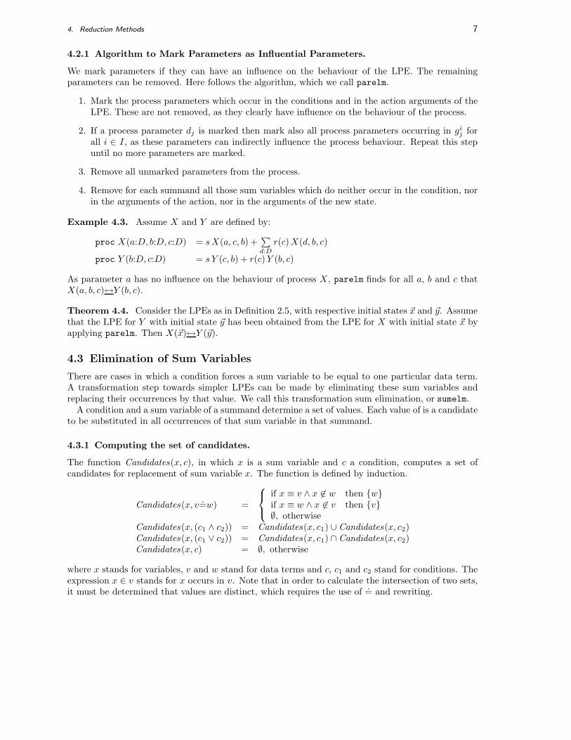
4.2.1 Algorithm to Mark Parameters as Influential Parameters.

We mark parameters if they can have an influence on the behaviour of the LPE. The remainingparameters can be removed. Here follows the algorithm, which we call parelm.

1. Mark the process parameters which occur in the conditions and in the action arguments of theLPE. These are not removed, as they clearly have influence on the behaviour of the process.

2. If a process parameter dj is marked then mark also all process parameters occurring in gij forall i ∈ I, as these parameters can indirectly influence the process behaviour. Repeat this stepuntil no more parameters are marked.

3. Remove all unmarked parameters from the process.

4. Remove for each summand all those sum variables which do neither occur in the condition, norin the arguments of the action, nor in the arguments of the new state.

Example 4.3. Assume X and Y are defined by:

proc X(a:D, b:D, c:D) = sX(a, c, b) +∑d:D

r(c)X(d, b, c)

proc Y (b:D, c:D) = s Y (c, b) + r(c)Y (b, c)

As parameter a has no influence on the behaviour of process X , parelm finds for all a, b and c thatX(a, b, c)↔Y (b, c).

Theorem 4.4. Consider the LPEs as in Definition 2.5, with respective initial states ~x and ~y. Assumethat the LPE for Y with initial state ~y has been obtained from the LPE for X with initial state ~x byapplying parelm. Then X(~x)↔Y (~y).

4.3 Elimination of Sum Variables

There are cases in which a condition forces a sum variable to be equal to one particular data term.A transformation step towards simpler LPEs can be made by eliminating these sum variables andreplacing their occurrences by that value. We call this transformation sum elimination, or sumelm.

A condition and a sum variable of a summand determine a set of values. Each value of is a candidateto be substituted in all occurrences of that sum variable in that summand.

4.3.1 Computing the set of candidates.

The function Candidates(x, c), in which x is a sum variable and c a condition, computes a set ofcandidates for replacement of sum variable x. The function is defined by induction.

Candidates(x, v .=w) =

if x ≡ v ∧ x 6∈ w then {w}if x ≡ w ∧ x 6∈ v then {v}∅, otherwise

Candidates(x, (c1 ∧ c2)) = Candidates(x, c1) ∪ Candidates(x, c2)Candidates(x, (c1 ∨ c2)) = Candidates(x, c1) ∩ Candidates(x, c2)Candidates(x, c) = ∅, otherwise

where x stands for variables, v and w stand for data terms and c, c1 and c2 stand for conditions. Theexpression x ∈ v stands for x occurs in v. Note that in order to calculate the intersection of two sets,it must be determined that values are distinct, which requires the use of .= and rewriting.

4. Reduction Methods 8

4.3.2 Substitution and Elimination.

For all i ∈ I, j ∈ 1 . . . ni, at which the set Candidates(eij , ci) is not empty (choose a value v from thisset), or the sort of eij contains exactly one element (call that element v):

1. Substitute v in all occurrences of eij in the ith summand of the LPE, and

2. Eliminate eij from the list of sum variables of the ith summand.

Example 4.5. Consider

proc X(d:Bool) =∑

b:Bool

a(b).X(b)/b .=f.δ

proc Y (d:Bool) = a(f).Y (f)/f.=f.δ

Sumelm yields X(d)↔Y (d). Rewriting the condition in Y makes it equal to t (true).

Theorem 4.6. Consider the LPEs as in Definition 2.5. Assume that the LPE for Y has beenobtained from the LPE for X by applying sumelm. Then, for state vector ~x it holds that X(~x)↔Y (~x).

4.4 An application of the reduction tools to an example

To demonstrate the cooperation of the three reduction algorithms, we take a slightly more substantialexample. The patterns which are found in this example occur often in bigger specifications afterlinearization.

sort Bool,Bit,Dfunc t, f:→ Bool, d1, d2 :→ D, 0, 1:→ Bitmap ¬ : Bool→ Bool, ∨ : Bool×Bool→ Bool

.=:D×D→ Bool, .=:Bit×Bit→ Boolvar b : Boolrew ¬t = f, ¬f = t, t ∨ b = t, f ∨ b = bvar d : Drew d1

.=d2 = f, d2.=d1 = f, d .=d = t

var b : Bitrew 0 .=1 = f, 1 .=0 = f, b .=b = tproc X(d:D, b:Bit)=

∑d0:D

τ X(d0, b) /d.=d2∨b .=0. δ+

∑b0:Bit

τ X(d, b0) /b0.=0. δ

init X(d1, 0)

• Algorithm parelm does not change the LPE, because the process parameters d and b occur inone of the conditions.

• Algorithm constelm does not change the LPE, because the sum variables d0 or b0 occur in bothprocess argument vectors.

• Algorithm sumelm changes the LPE. It substitutes 0 in each occurrence of sum variable b0 andremoves that sum variable. The equation becomes

proc X(d:D, b:Bit) =∑d0:D

τ X(d0, b) /d.=d2∨b .=0. δ + τ X(d, 0) /0 .=0. δ

init X(d1, 0)

• Algorithm parelm still cannot change the modified LPE.

• Algorithm constelm changes the LPE. It substitutes 0 in each occurrence of b and removes thatparameter. The equation becomes

4. Reduction Methods 9

proc X(d:D) =∑d0:D

τ X(d0) /d .=d2 ∨ 0 .=0. δ + τ X(d) /0 .=0. δ

init X(d1)

• After rewriting the equation becomes

proc X(d:D) =∑d0:D

τ X(d0) / t. δ + τ X(d) / t. δ

init X(d1)

• Algorithm parelm changes the LPE. Process parameter d does not occur in the condition.Process parameter d will be removed. Sum variable d0 does not occur in the equation. Sumvariable d0 will be removed.

proc X() = τ X() / t. δ + τ X() / t. δinit X()

The state space is reduced from two states to one state, a reduction of 50 per cent.

4.5 Elimination of Structured Variables

There are possible reductions of an LPE which are not detected by the previously mentioned reductionmethods because the required properties of the variables are hidden within complex data terms. Wedescribe here an expansion method, which replaces terms with a constructor function as head symbolsby the name of the constructor and its arguments. In this way variables occuring in subterms arebetter exposed and more amenable to be eliminated by one of the other tools. For instance, a listexpression in(v, l) is split into the value in, and terms v and l, and a list expression nil is replacedby the value nil . Consequently, a variable of sort List is replaced by three variables. The first one toindicate whether the head symbol of the term represented by the variable starts with in or nil andtwo to represents the two arguments in case the term starts with in . We call this expansion methodstructelm, short for structure elimination.

4.5.1 Unfolding a Structured Sort S.

1. Detect how many constructors generate S. Assume that S is generated by k constructorsfi: D1

i × · · · ×Dmii → S, with 1 ≤ i ≤ k.

2. Add a new enumerated sort Uk with k constant constructors, c1, . . . , ck, to the abstract datatype. The elements of Uk represent each a different constructor of sort S.

3. Add a function C: Uk × S × · · · × S → S to the abstract data type with arity k + 1. Add thefollowing rewrite rules to the abstract data type.

rew C(ci, x1, . . . , xi, . . . , xk) = xiC(e, x . . . , x) = x

These functions C are called case functions. Note that strictly spoken the last rewrite rule isnot necessary, but it sometimes turns out to be useful.

4. Add projection functions det : S → Uk and πji : S → Dji with 1 ≤ j ≤ mi and 1 ≤ i ≤ k to the

abstract data type. Add the following rewrite rules to the abstract data type.

rew det(fi(d1i , . . . , d

ji , . . . , d

mii )) = ci

πji (fi(d1i , . . . , d

ji , . . . , d

mii )) = dji

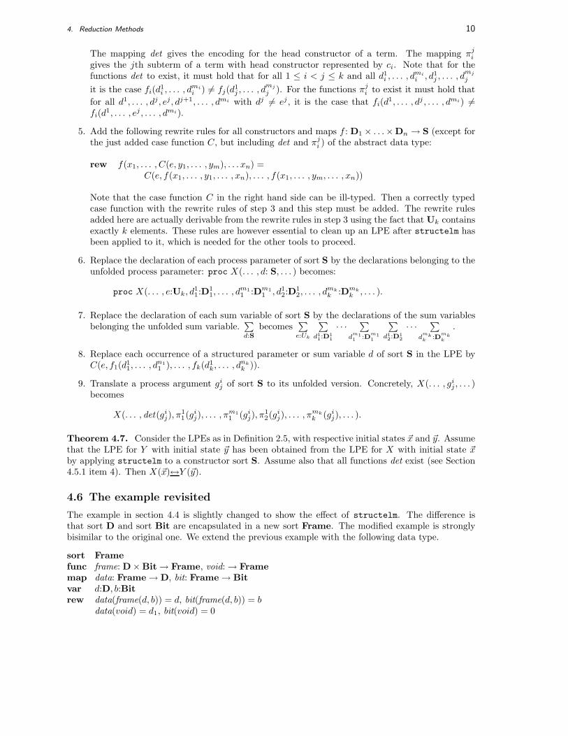
4. Reduction Methods 10

The mapping det gives the encoding for the head constructor of a term. The mapping πjigives the jth subterm of a term with head constructor represented by ci. Note that for thefunctions det to exist, it must hold that for all 1 ≤ i < j ≤ k and all d1

i , . . . , dmii , d1

j , . . . , dmjj

it is the case fi(d1i , . . . , d

mii ) 6= fj(d1

j , . . . , dmjj ). For the functions πji to exist it must hold that

for all d1, . . . , dj , ej , dj+1, . . . , dmi with dj 6= ej , it is the case that fi(d1, . . . , dj , . . . , dmi) 6=fi(d1, . . . , ej , . . . , dmi).

5. Add the following rewrite rules for all constructors and maps f : D1 × . . .×Dn → S (except forthe just added case function C, but including det and πji ) of the abstract data type:

rew f(x1, . . . , C(e, y1, . . . , ym), . . . xn) =C(e, f(x1, . . . , y1, . . . , xn), . . . , f(x1, . . . , ym, . . . , xn))

Note that the case function C in the right hand side can be ill-typed. Then a correctly typedcase function with the rewrite rules of step 3 and this step must be added. The rewrite rulesadded here are actually derivable from the rewrite rules in step 3 using the fact that Uk containsexactly k elements. These rules are however essential to clean up an LPE after structelm hasbeen applied to it, which is needed for the other tools to proceed.

6. Replace the declaration of each process parameter of sort S by the declarations belonging to theunfolded process parameter: proc X(. . . , d: S, . . . ) becomes:

proc X(. . . , e:Uk, d11:D1

1, . . . , dm11 :Dm1

1 , d12:D1

2, . . . , dmkk :Dmk

k , . . . ).

7. Replace the declaration of each sum variable of sort S by the declarations of the sum variablesbelonging the unfolded sum variable.

∑d:S

becomes∑e:Uk

∑d1

1:D11

· · ·∑

dm11 :D

m11

∑d1

2:D12

· · ·∑

dmkk :D

mkk

.

8. Replace each occurrence of a structured parameter or sum variable d of sort S in the LPE byC(e, f1(d1

1, . . . , dn11 ), . . . , fk(d1

k, . . . , dnkk )).

9. Translate a process argument gij of sort S to its unfolded version. Concretely, X(. . . , gij , . . . )becomes

X(. . . , det(gij), π11(gij), . . . , π

m11 (gij), π

12(gij), . . . , π

mkk (gij), . . . ).

Theorem 4.7. Consider the LPEs as in Definition 2.5, with respective initial states ~x and ~y. Assumethat the LPE for Y with initial state ~y has been obtained from the LPE for X with initial state ~xby applying structelm to a constructor sort S. Assume also that all functions det exist (see Section4.5.1 item 4). Then X(~x)↔Y (~y).

4.6 The example revisited

The example in section 4.4 is slightly changed to show the effect of structelm. The difference isthat sort D and sort Bit are encapsulated in a new sort Frame. The modified example is stronglybisimilar to the original one. We extend the previous example with the following data type.

sort Framefunc frame: D×Bit→ Frame, void:→ Framemap data: Frame→ D, bit: Frame→ Bitvar d:D, b:Bitrew data(frame(d, b)) = d, bit(frame(d, b)) = b

data(void) = d1, bit(void) = 0

5. Cooperation and influence of reductions 11

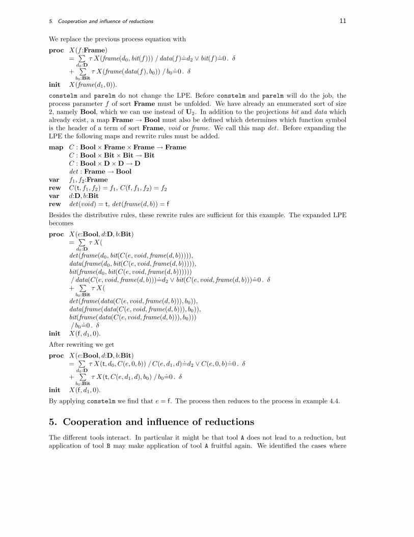
We replace the previous process equation with

proc X(f :Frame)=∑d0:D

τ X(frame(d0, bit(f))) /data(f) .=d2 ∨ bit(f) .=0. δ

+∑

b0:Bit

τ X(frame(data(f), b0)) /b0.=0. δ

init X(frame(d1, 0)).

constelm and parelm do not change the LPE. Before constelm and parelm will do the job, theprocess parameter f of sort Frame must be unfolded. We have already an enumerated sort of size2, namely Bool, which we can use instead of U2. In addition to the projections bit and data whichalready exist, a map Frame → Bool must also be defined which determines which function symbolis the header of a term of sort Frame, void or frame. We call this map det . Before expanding theLPE the following maps and rewrite rules must be added.

map C : Bool× Frame× Frame→ FrameC : Bool×Bit×Bit→ BitC : Bool×D×D→ Ddet : Frame→ Bool

var f1, f2:Framerew C(t, f1, f2) = f1, C(f, f1, f2) = f2

var d:D, b:Bitrew det(void) = t, det(frame(d, b)) = f

Besides the distributive rules, these rewrite rules are sufficient for this example. The expanded LPEbecomes

proc X(e:Bool, d:D, b:Bit)=∑d0:D

τ X(

det(frame(d0, bit(C(e, void, frame(d, b))))),data(frame(d0, bit(C(e, void, frame(d, b))))),bit(frame(d0, bit(C(e, void, frame(d, b))))))/data(C(e, void, frame(d, b))) .=d2 ∨ bit(C(e, void, frame(d, b))) .=0. δ+∑

b0:Bit

τ X(

det(frame(data(C(e, void, frame(d, b))), b0)),data(frame(data(C(e, void, frame(d, b))), b0)),bit(frame(data(C(e, void, frame(d, b))), b0)))/b0

.=0. δinit X(f, d1, 0).

After rewriting we get

proc X(e:Bool, d:D, b:Bit)=∑d0:D

τ X(t, d0, C(e, 0, b)) /C(e, d1, d) .=d2 ∨ C(e, 0, b) .=0. δ

+∑

b0:Bit

τ X(t, C(e, d1, d), b0) / b0.=0. δ

init X(f, d1, 0).

By applying constelm we find that e = f. The process then reduces to the process in example 4.4.

5. Cooperation and influence of reductions

The different tools interact. In particular it might be that tool A does not lead to a reduction, butapplication of tool B may make application of tool A fruitful again. We identified the cases where

6. Experimental results 12

this is the case and put these in Table 1. Horizontally, the tools can be found that do not lead to a

structelm sumelm parelm constelm

structelm X Yes Yes Yessumelm No X Yes Yesparelm No No X No

constelm No Yes Yes X

Table 1: Dependence of tools

reduction, but may become effective after applying one of the tools put vertically. So, for instance, thetable indicates that if structelm is applied when sumelm does not yield any reduction, then applyingsumelm after structelm might yield additional reductions. We put X’s on the diagonal, because thesepositions have no meaning.

Note that iteratively applying the same tool is only useful for structelm. But if there are norecursive types, then only a finite number of applications of structelm can take place.

6. Experimental results

Bounded retransmission protocolbefore reduction after reduction

l # states # transitions time # states # transitions time1 454 518 1.34s 454 518 1.45s2 1856 2134 2.02s 834 954 1.65s3 10550 12170 6.28s 1202 1378 1.89s4 86968 100406 44.09s 2224 2558 2.49s5 968538 1118498 8m27.13s 8642 9970 6.45s

Onebit sliding window protocolbefore reduction after reduction

n # states # transitions time # states # transitions time1 39577 229650 21.19s 39577 229650 20.42s2 319912 1937388 3m44.29s 39577 229650 19.37s3 1208737 7484714 29m56.95s 39577 229650 18.79s

Firewire link layer protocolbefore reduction after reduction

n # states # transitions time # states # transitions time1 95160 158017 17m15.58s 74271 123370 59m31.00s2 371804 641565 1h9m15.30s 74271 145456 1h0m1.79s3 872224 1548401 2h22m18.41s 74271 167542 59m56.56s

Table 2: The effect of the elimination tools on the size of state spaces

We applied our reduction techniques to a number of data transfer protocols that have been describedin µCRL. These are the bounded retransmission protocol [9], the one bit sliding window protocol [3]and the Firewire link layer protocol [13]. These protocols are quite different in nature. For all protocolswe hid the delivery of data, in order to investigate the control structure. By applying the different

References 13

elimination algorithms we were able to remove most or even all occurrences of variables refering todata reducing the state space substantially. If all variables refering to data are removed, results onthe control structure hold for any data domain, in particular for those of infinite size.

In the tables we list the sizes of the state spaces for different sizes of the data domain. For thebounded retransmission protocol the length of the data packages and the number of data elements isgiven by l and the number of retransmissions has been set to 3. For the two other protocols the numberof data elements is given by n. The one bit sliding window protocol is a unidirectional sliding windowprotocol with buffer size 1 at both the sending and receiving sides. The Firewire link layer protocolconsists of a bus and two link processes. The results have been obtained on a SGI Powerchallengewith R12000 processors on 300Mhz. The version of the toolset that has been used is 2.8.3.

6.0.1 Acknowledgments.

We thank Jaco van de Pol for his comments on this paper.

References

1. M.G.J. van den Brand, P. Klint, and P.A. Olivier. Compilation and Memory Management forASF+SDF. In: Proceedings in Compiler Construction (CC’99) (ed. S. Jahnichen), LNCS 1575,198–213, Springer-Verlag, 1999.

2. J.A. Bergstra and J.W. Klop. Process algebra for synchronous communication. Information andCommunication, 60(1/3):109-137,1984.

3. M.A. Bezem and J.F. Groote. A correctness proof of a one bit sliding window protocol in µCRL.The Computer Journal, 37(4): 289-307, 1994.

4. S.C.C. Blom. Verification of the Euris railway control specification of Woerden-Harmelen. Workin progress. Centrum voor Wiskunde en Informatica, Amsterdam, 2000

5. S.C.C. Blom. Partial τ -confluence for efficient state space generation. Technical report, CWI,2001; to appear.

6. W.J. Fokkink. Introduction to Process Algebra, In Texts in Theoretical Computer Science, AnEATCS Series. Springer-Verlag, 2000.

7. H. Garavel. OPEN/CAESAR: An Open Software Architecture for Verification, Simulation, and Test-ing”. In G. Goos, J. Hartmanis, and J. van Leeuwen, Editors, Proceedings of TACAS’98, volume1384 of Lecture Notes in Computer Science, Springer Verlag, pages 68-84, 1998. Available fromhttp://www.inrialpes.fr/vasy/Publications.

8. J.F. Groote. The syntax and semantics of timed µCRL. Report SEN-R9709. CWI, The Nether-lands, 1997.

9. J.F. Groote and J.C. van de Pol. A bounded retransmission protocol for large data packets. Acase study in computer checked verification. In M. Wirsing and M. Nivat, Editors, Proceedings ofAMAST’96, Munich, volume 1101 of Lecture Notes in Computer Science, Springer Verlag, pages536-550, 1996.

10. J.F. Groote and A. Ponse. The Syntax and Semantics of µCRL. In A. Ponse and C. Verhoef andS.F.M. van Vlijmen,editors, Workshops in Computing, pages 26–62. Springer-Verlag, 1994.

11. J.F. Groote, A. Ponse and Y.S. Usenko. Linearization in parallel pCRL. Journal of Logic andAlgebraic Programming, 48(1-2):39-72, 2001.

12. J.F. Groote and M.P.A. Sellink. Confluence for Process Verification. In Theoretical ComputerScience B (Logic, semantics and theory of programming), 170(1-2):47-81, 1996.

References 14

13. S.P. Luttik. Description and formal specification of the link layer of P1394. Technical Report SEN-R9706, CWI, Amsterdam, 1997. ftp://ftp.cwi.nl/pub/CWIreports/SEN/SEN-R9706.ps.Z

14. J.C. van de Pol. A Prover for the µCRL Toolset with Applications – version 0.1. Technical reportSEN-R0106, CWI, Amsterdam, 2001.

15. Y.S. Usenko. Linearization of µCRL processes. To appear. 2001.

16. M. Wirsing. Algebraic specification. In J. van Leeuwen, editor, Handbook of Theoretical ComputerScience, volume II, pages 677–788. Elsevier Science Publishers B.V., 1990.

17. A.G. Wouters Manual for the µCRL toolset (version 2.07). Technical report, CWI, 2001; toappear. Available at http://www.cwi.nl/∼mcrl

A. The µCRL Toolset runs the Example 15

A. The µCRL Toolset runs the Example

We show how we applied to µCRL toolset to the running example.

sort Dfunc d1,d2: -> Dmap eq:D#D -> Boolrew eq(d1,d1)=T eq(d2,d2)=T eq(d1,d2)=F eq(d2,d1)=F

sort Boolmap and,or:Bool#Bool -> Bool

not:Bool -> Booleq:Bool#Bool->Bool

func T,F:-> Bool

var x:Boolrew and(T,x)=x and(x,T)=x and(x,F)=F and(F,x)=F

or(T,x)=T or(x,T)=T or(x,F)=x or(F,x)=xnot(F)=T not(T)=Feq(x,T)=x eq(T,x)=x eq(F,x)=not(x) eq(x,F)=not(x)

sort Bitfunc 0,1:-> Bitmap eq:Bit#Bit -> Boolrew eq(0,0)=T eq(1,1)=T eq(0,1)=F eq(1,0)=F

sort Framefunc frame:D#Bit -> Frame

void:->Framemap data:Frame -> D

bit:Frame -> Bitvar d:D b:Bitrew data(void)=d1 data(frame(d,b)) =d

bit(void)=0 bit(frame(d,b))=b

proc X(f:Frame) = sum(d0:D,tau.X(frame(d0, bit(f)))<|or(eq(data(f),d2), eq(bit(f),0))|>delta)

+ sum(b0:Bit,tau.X(frame(data(f),b0))<|eq(b0,0)|>delta)

init X(frame(d1,0))

Most µCRL commands [17] are filters which read from stdin and write to stdout, so they can beused in a pipeline. The reduced LPE is written to the file output. Internally LPEs are input andoutput in a compressed format, called the tbf format. The pretty printer, pp, is used to transform tbffiles to a readable form. Below the command is given that transforms the example, followed by itsoutput.

mcrl -stdout -regular -nocluster input|structelm -expand Frame|rewr -case| \sumelm|constelm|parelm|pp > output

A. The µCRL Toolset runs the Example 16

Structelm: Generated casefunction: C2-Frame(Bool,Frame,Frame)Structelm: Parameter f: "Frame" is expanded to 3 parametersStructelm: Number of parameters of input LPE: 1Structelm: Number of parameter(s) of output LPE:3Rewr: structelm -case-completion has ended successfullyRewr: NOW COMPILINGRewr: gcc -O4 -DNDEBUG -c REWRITERALT.c -o REWRITER.oRewr: COMPILING FINISHEDRewr: gcc -shared REWRITER.o -o REWRITER.soRewr: REWRITER LOADEDRewr: Read 2 summandsRewr: Written 2 summandsSumelm: NOW COMPILINGSumelm: gcc -O4 -DNDEBUG -c REWRITERALT.c -o REWRITER.oSumelm: COMPILING FINISHEDSumelm: gcc -shared REWRITER.o -o REWRITER.soSumelm: REWRITER LOADEDSumelm: Read 2 summandsSumelm: Number of parameters of input LPE: 3Sumelm: Summand 2: substituted for "b0" the term 0Sumelm: In this summand is (are) 1 variable(s) eliminatedSumelm: Written 2 summandsSumelm: Number of parameters of output LPE: 3Constelm: NOW COMPILINGConstelm: gcc -O4 -DNDEBUG -c REWRITERALT.c -o REWRITER.oConstelm: COMPILING FINISHEDConstelm: gcc -shared REWRITER.o -o REWRITER.soConstelm: REWRITER LOADEDConstelm: Read 2 summandsConstelm: Number of parameters of input LPE: 3Constelm: Constant parameter "f_e" (pos 1, sort "Bool") = "F" is removedConstelm: Constant parameter "f_1" (pos 3, sort "Bit") = "0" is removedConstelm: Number of removed parameter(s):2Constelm: Number of remaining parameter(s) of output LPE:1Constelm: Written 2 summandsConstelm: Number of parameters of output LPE: 1Parelm: Number of parameters of input LPE: 1Parelm: Parameter "f_0" (sort "D") is removedParelm: In total 1 process parameter has been removedParelm: Variable "d0" (sort "D") in the sum operator of summand 1 has been deletedParelm: Number of parameters of output LPE: 0

The computed reduced LPE can be found in the file output and looks as follows.

proc X =tau. X <|T|>delta+tau. X <|T|>deltainit X