Centre national de la recherche scientifique · Université de Bourgogne , U.F.R Sciences et...
325
Université de Bourgogne , U.F.R Sciences et techniques Institut de Mathématiques de Bourgogne Ecole doctorale Carnot-Pasteur THÈSE pour l’obtention du grade de Docteur de l’Université de Bourgogne en Mathématiques présentée et soutenue publiquement par Antoine Godichon-Baggioni le 17 Juin 2016 Algorithmes stochastiques pour la statistique robuste en grande dimension Directeurs de thèse : Hervé Cardot, Peggy Cénac Jury composé de Hervé Cardot Université de Bourgogne Directeur Peggy Cénac Université de Bourgogne Co-encadrante Antonio Cuevas Universidad Autónoma de Madrid Rapporteur Clément Dombry Université de Franche-Comté Examinateur Anatoli Juditsky Université Joseph Fourier Rapporteur Mariane Pelletier Université de Versailles Examinatrice Anne Ruiz-Gazen Université de Toulouse 1 Examinatrice
Transcript of Centre national de la recherche scientifique · Université de Bourgogne , U.F.R Sciences et...

Université de Bourgogne , U.F.R Sciences et techniquesInstitut de Mathématiques de Bourgogne
Ecole doctorale Carnot-Pasteur
THÈSE
pour l’obtention du grade de
Docteur de l’Université de Bourgogne
en Mathématiques
présentée et soutenue publiquement par
Antoine Godichon-Baggioni
le 17 Juin 2016
Algorithmes stochastiques pour la statistique robusteen grande dimension
Directeurs de thèse : Hervé Cardot, Peggy Cénac
Jury composé de
Hervé Cardot Université de Bourgogne DirecteurPeggy Cénac Université de Bourgogne Co-encadranteAntonio Cuevas Universidad Autónoma de Madrid RapporteurClément Dombry Université de Franche-Comté ExaminateurAnatoli Juditsky Université Joseph Fourier RapporteurMariane Pelletier Université de Versailles ExaminatriceAnne Ruiz-Gazen Université de Toulouse 1 Examinatrice


A Nénette et Toussaint


Remerciements
Je tiens tout d’abord à remercier mes directeurs de thèse, Hervé Cardot et Peggy Cénac.Merci à Peggy pour toute l’aide apportée durant toutes ces années, et de m’avoir appuyépour que je puisse faire cette thèse. Un grand merci à Hervé d’avoir accepté de diriger cettethèse. Enfin, merci à tous les deux d’avoir été aussi patients, d’avoir parfaitement su orientermon travail, et de toujours avoir vos portes ouvertes pour mes (très) nombreuses questions.
Je tiens aussi à remercier Bruno Portier, non seulement pour avoir accepté de travailleravec moi, ce qui m’a ouvert de nombreuses perspectives de recherche, mais aussi pourses nombreux conseils avisés. J’apprécie énormément nos fréquentes discussions grâce aux-quelles je peux prendre davantage de recul sur mon travail.
Antonio Cuevas et Anatoli Juditsky m’ont fait l’honneur d’accepter de rapporter mathèse et de faire parti du Jury, je les remercie pour cela ainsi que pour leurs précieuses re-marques, notamment bibliographiques, qui m’ont permis d’améliorer mon manuscrit et quim’ouvrent de nombreuses perspectives. Je remercie aussi Clément Dombry, Mariane Pelle-tier, Bruno Portier et Anne Ruiz-Gazen, qui me font l’honneur de faire partie de mon Jury.
Faire une thèse est une chance, mais la faire dans de si bonnes conditions est véritable-ment un luxe, et cela je le dois à tous les personnels du laboratoire, Anissa, Aziz, Caro, Fran-cis, Magalie, Nadia, Sébastien, Véronique, mais aussi aux enseignants-chercheurs de l’IMB.Merci aussi à tous les doctorants et à l’association des Doctorants en Mathématiques de Di-jon pour tous ces bons moments, les exposés, les pots... Enfin merci à tous mes co-bureaux,Adriana, Armand, Bachar, Bruno, Charlie, Jessie, Michael, Rebecca et Simone d’avoir toléréla musique, les ronchonnements.... Merci aussi à mes co-brasseurs, Charlie, Jérémy et Rémi.
Si je suis en train d’écrire ces remerciements, c’est aussi parce que des personnes m’ontaidé à des moments cruciaux, ou m’ont prodigué de très bon conseils. Donc merci à Charliepour ces précieux avis, et merci à tous ceux qui m’ont gracieusement aidé à préparer l’Agré-gation (Peggy Cénac, Shizan Fang, Lucy Moser, Emmanuel Wagner, ...) et m’ont aidé, par lamême occasion, à retrouver des bases solides dont j’ai eu besoin tout au long de ma thèse.
5

Je tiens à remercier toute ma famille, mes parents pour leurs bons (et mauvais) choix grâceauxquels j’en suis là aujourd’hui, mon frère et ma soeur, pour m’avoir supporté toutes sesannées, mes grand-mères, mes oncles et tantes, mes cousins... Merci à mon père et à MamoPaula pour les corrections orthographiques, merci à ma mère et ma tante Louise pour leursconseils pendant ces trois dernières années.
Grazie a tutti i Zalaninchi pour votre présence et votre soutien. Merci à tous les membresde l’Association Sportive Sociale et Culturelle de Zalana (Antho G, Antho T, Audrey, Clé-ment, Juju, Ludo, Mika, Roland, Romane, Mareva,...), merci à tous mes cousins. Bref, mercià tous et a prestu !
Il y a des moments dans la vie qui sont déterminants, et je remercie Rebecca de m’avoiraidé à saisir les occasions qui se sont offertes à moi ainsi que de m’avoir encouragé à fairecette thèse.
Enfin, mes derniers remerciements vont à mon oncle Toussaint et à ma tante Nénette, àqui je dédie cette thèse. Malgré la distance, vous avez toujours été présents dans ma vie etsoucieux de mon avenir. Malheureusement, je ne pourrais pas partager cette dernière lignedroite avec vous. J’ose espérer que vous auriez été fiers de moi.
Résumé
Cette thèse porte sur l’étude d’algorithmes stochastiques en grande dimension ainsi qu’àleur application en statistique robuste. Dans la suite, l’expression grande dimension pourraaussi bien signifier que la taille des échantillons étudiés est grande ou encore que les va-riables considérées sont à valeurs dans des espaces de grande dimension (pas nécessaire-ment finie). Afin d’analyser ce type de données, il peut être avantageux de considérer desalgorithmes qui soient rapides, qui ne nécessitent pas de stocker toutes les données, et quipermettent de mettre à jour facilement les estimations. Dans de grandes masses de donnéesen grande dimension, la détection automatique de points atypiques est souvent délicate. Ce-pendant, ces points, même s’ils sont peu nombreux, peuvent fortement perturber des indica-teurs simples tels que la moyenne ou la covariance. On va se concentrer sur des estimateursrobustes, qui ne sont pas trop sensibles aux données atypiques.
Dans une première partie, on s’intéresse à l’estimation récursive de la médiane géomé-trique, un indicateur de position robuste, et qui peut donc être préférée à la moyenne lors-qu’une partie des données étudiées est contaminée. Pour cela, on introduit un algorithme deRobbins-Monro ainsi que sa version moyennée, avant de construire des boules de confiancenon asymptotiques et d’exhiber leurs vitesses de convergence Lp et presque sûre.
La deuxième partie traite de l’estimation de la "Median Covariation Matrix" (MCM), quiest un indicateur de dispersion robuste lié à la médiane, et qui, si la variable étudiée suit uneloi symétrique, a les mêmes sous-espaces propres que la matrice de variance-covariance. Cesdernières propriétés rendent l’étude de la MCM particulièrement intéressante pour l’Analyseen Composantes Principales Robuste. On va donc introduire un algorithme itératif qui per-met d’estimer simultanément la médiane géométrique et la MCM ainsi que les q principauxvecteurs propres de cette dernière. On donne, dans un premier temps, la forte consistancedes estimateurs de la MCM avant d’exhiber les vitesses de convergence en moyenne quadra-tique.
Dans une troisième partie, en s’inspirant du travail effectué sur les estimateurs de la mé-diane et de la "Median Covariation Matrix", on exhibe les vitesses de convergence presque
7

sûre et Lp des algorithmes de gradient stochastiques et de leur version moyennée dans desespaces de Hilbert, avec des hypothèses moins restrictives que celles présentes dans la litté-rature. On présente alors deux applications en statistique robuste : estimation de quantilesgéométriques et régression logistique robuste.
Dans la dernière partie, on cherche à ajuster une sphère sur un nuage de points répar-tis autour d’une sphère complète où tronquée. Plus précisément, on considère une variablealéatoire ayant une distribution sphérique tronquée, et on cherche à estimer son centre ainsique son rayon. Pour ce faire, on introduit un algorithme de gradient stochastique projeté etson moyenné. Sous des hypothèses raisonnables, on établit leurs vitesses de convergence enmoyenne quadratique ainsi que la normalité asymptotique de l’algorithme moyenné.
Mots-clés : Grande Dimension, Données Fonctionnelles, Algorithmes Stochastiques, Algo-rithmes Récursifs, Algorithmes de Gradient Stochastiques, Moyennisation, Statistique Ro-buste, Médiane Géométrique.

Abstract
This thesis focus on stochastic algorithms in high dimension as well as their applicationin robust statistics. In what follows, the expression high dimension may be used when thethe size of the studied sample is large or when the variables we consider take values in highdimensional spaces (not necessarily finite). In order to analyze these kind of data, it can beinteresting to consider algorithms which are fast, which do not need to store all the data, andwhich allow to update easily the estimates. In large sample of high dimensional data, outliersdetection is often complicated. Nevertheless, these outliers, even if they are not many, canstrongly disturb simple indicators like the mean and the covariance. We will focus on robustestimates, which are not too much sensitive to outliers.
In a first part, we are interested in the recursive estimation of the geometric median,which is a robust indicator of location which can so be preferred to the mean when a part ofthe studied data is contaminated. For this purpose, we introduce a Robbins-Monro algorithmas well as its averaged version, before building non asymptotic confidence balls for theseestimates, and exhibiting their Lp and almost sure rates of convergence.
In a second part, we focus on the estimation of the Median Covariation Matrix (MCM),which is a robust dispersion indicator linked to the geometric median. Furthermore, if thestudied variable has a symmetric law, this indicator has the same eigenvectors as the cova-riance matrix. This last property represent a real interest to study the MCM, especially forRobust Principal Component Analysis. We so introduce a recursive algorithm which enablesus to estimate simultaneously the geometric median, the MCM, and its q main eigenvectors.We give, in a first time, the strong consistency of the estimators of the MCM, before exhibitingtheir rates of convergence in quadratic mean.
In a third part, in the light of the work on the estimates of the median and of the MedianCovariation Matrix, we exhibit the almost sure and Lp rates of convergence of averagedstochastic gradient algorithms in Hilbert spaces, with less restrictive assumptions than in theliterature. Then, two applications in robust statistics are given : estimation of the geometricquantiles and application in robust logistic regression.
9

In the last part, we aim to fit a sphere on a noisy points cloud spread around a completeor truncated sphere. More precisely, we consider a random variable with a truncated sphe-rical distribution, and we want to estimate its center as well as its radius. In this aim, weintroduce a projected stochastic gradient algorithm and its averaged version. We establishthe strong consistency of these estimators as well as their rates of convergence in quadraticmean. Finally, the asymptotic normality of the averaged algorithm is given.
Keywords High Dimension, Functional Data, Stochastic Algorithms, Recursive Algorithms,Stochastic Gradient Algorithms, Averaging, Robust Statistics, Geometric Median.

Table des matières
Introduction 19
1 Quelques résultats sur les algorithmes stochastiques 231.1 Algorithmes déterministes . . . . . . . . . . . . . . . . . . . . . . . . . . . . . . 24
1.1.1 Recherche des zéros d’une fonction . . . . . . . . . . . . . . . . . . . . 241.1.2 Recherche des minima d’une fonction . . . . . . . . . . . . . . . . . . . 27
1.2 Algorithmes de gradient stochastiques . . . . . . . . . . . . . . . . . . . . . . . 281.2.1 Définition et premiers résultats . . . . . . . . . . . . . . . . . . . . . . . 281.2.2 Vitesses de convergence . . . . . . . . . . . . . . . . . . . . . . . . . . . 321.2.3 Algorithme projeté . . . . . . . . . . . . . . . . . . . . . . . . . . . . . . 38
1.3 L’algorithme moyenné . . . . . . . . . . . . . . . . . . . . . . . . . . . . . . . . 411.3.1 Retour sur l’algorithme de Robbins-Monro . . . . . . . . . . . . . . . . 411.3.2 Définition et comportement asymptotique . . . . . . . . . . . . . . . . 421.3.3 Vitesse de convergence en moyenne quadratique . . . . . . . . . . . . 45
2 Introduction à la notion de robustesse 472.1 Introduction . . . . . . . . . . . . . . . . . . . . . . . . . . . . . . . . . . . . . . 47
2.1.1 Une première définition de la robustesse . . . . . . . . . . . . . . . . . 482.2 M-estimateurs . . . . . . . . . . . . . . . . . . . . . . . . . . . . . . . . . . . . . 49
2.2.1 L’estimateur du Maximum de Vraisemblance . . . . . . . . . . . . . . . 502.2.2 M-estimateurs . . . . . . . . . . . . . . . . . . . . . . . . . . . . . . . . . 50
2.3 Comportement asymptotique des M-estimateurs de position . . . . . . . . . . 512.3.1 Cas unidimensionnel . . . . . . . . . . . . . . . . . . . . . . . . . . . . . 512.3.2 Cas multidimensionnel . . . . . . . . . . . . . . . . . . . . . . . . . . . 532.3.3 Exemples . . . . . . . . . . . . . . . . . . . . . . . . . . . . . . . . . . . 54
2.4 Comment construire un M-estimateur . . . . . . . . . . . . . . . . . . . . . . . 552.4.1 Estimateur de position dans R . . . . . . . . . . . . . . . . . . . . . . . 552.4.2 Cas multidimensionnel . . . . . . . . . . . . . . . . . . . . . . . . . . . 56

12 TABLE DES MATIÈRES
2.5 Fonction d’influence . . . . . . . . . . . . . . . . . . . . . . . . . . . . . . . . . 57
2.5.1 Définition . . . . . . . . . . . . . . . . . . . . . . . . . . . . . . . . . . . 57
2.5.2 Fonction d’influence d’un M-estimateur . . . . . . . . . . . . . . . . . . 58
2.5.3 Exemples . . . . . . . . . . . . . . . . . . . . . . . . . . . . . . . . . . . 59
2.6 Biais asymptotique maximum et point de rupture . . . . . . . . . . . . . . . . 60
2.6.1 Définitions . . . . . . . . . . . . . . . . . . . . . . . . . . . . . . . . . . . 60
2.6.2 Exemples . . . . . . . . . . . . . . . . . . . . . . . . . . . . . . . . . . . 61
3 Synthèse des principaux résultats 653.1 Estimation de la médiane : boules de confiance . . . . . . . . . . . . . . . . . . 65
3.1.1 Définitions et hypothèses . . . . . . . . . . . . . . . . . . . . . . . . . . 65
3.1.2 Vitesses de convergence de l’algorithme de type Robbins-Monro . . . 66
3.1.3 Boules de confiance non asymptotiques . . . . . . . . . . . . . . . . . . 67
3.2 Estimation de la médiane : vitesses de convergence Lp et presque sûre . . . . 69
3.2.1 Décomposition de l’algorithme de type Robbins-Monro . . . . . . . . . 69
3.2.2 Vitesses de convergence Lp des algorithmes . . . . . . . . . . . . . . . 69
3.2.3 Vitesses de convergence presque sûre des algorithmes . . . . . . . . . 71
3.3 Estimation de la "Median Covariation Matrix" . . . . . . . . . . . . . . . . . . 72
3.3.1 Définition et hypothèses . . . . . . . . . . . . . . . . . . . . . . . . . . . 72
3.3.2 Les algorithmes . . . . . . . . . . . . . . . . . . . . . . . . . . . . . . . . 73
3.3.3 Résultats de convergence . . . . . . . . . . . . . . . . . . . . . . . . . . 74
3.4 Vitesse de convergence des algorithmes de Robbins-Monro et de leur moyenné 75
3.4.1 Hypothèses . . . . . . . . . . . . . . . . . . . . . . . . . . . . . . . . . . 75
3.4.2 Vitesses de convergence . . . . . . . . . . . . . . . . . . . . . . . . . . . 77
3.4.3 Applications . . . . . . . . . . . . . . . . . . . . . . . . . . . . . . . . . . 78
3.5 Estimation des paramètres d’une distribution sphérique tronquée . . . . . . . 79
3.5.1 Cadre de travail . . . . . . . . . . . . . . . . . . . . . . . . . . . . . . . . 80
3.5.2 Les algorithmes . . . . . . . . . . . . . . . . . . . . . . . . . . . . . . . . 81
3.5.3 Vitesses de convergence . . . . . . . . . . . . . . . . . . . . . . . . . . . 82
I Estimation récursive de la médiane géométrique dans les espaces de Hilbert 85
4 Estimation of the geometric median : non asymptotic confidence balls 874.1 Introduction . . . . . . . . . . . . . . . . . . . . . . . . . . . . . . . . . . . . . . 89
4.2 Assumptions on the median and convexity properties . . . . . . . . . . . . . . 91
4.3 Rates of convergence of the Robbins-Monro algorithms . . . . . . . . . . . . . 93

TABLE DES MATIÈRES 13
4.4 Non asymptotic confidence balls . . . . . . . . . . . . . . . . . . . . . . . . . . 954.4.1 Non asymptotic confidence balls for the Robbins-Monro algorithm . . 954.4.2 Non asymptotic confidence balls for the averaged algorithm : . . . . . 98
4.5 Proofs . . . . . . . . . . . . . . . . . . . . . . . . . . . . . . . . . . . . . . . . . . 1004.5.1 Proof of Theorem 4.3.1 . . . . . . . . . . . . . . . . . . . . . . . . . . . . 1004.5.2 Proof of Theorem 4.4.2 . . . . . . . . . . . . . . . . . . . . . . . . . . . . 109
A Estimation of the geometric median : confidence balls. Appendix 111A.1 Decomposition of the Robbins-Monro algorithm . . . . . . . . . . . . . . . . . 112A.2 Proof of technical lemma and of Proposition 4.3.1 . . . . . . . . . . . . . . . . 112A.3 Proofs of Proposition 4.4.1 and Theorem 4.4.1 . . . . . . . . . . . . . . . . . . . 117
5 Estimating the geometric median : Lp and almost sure rates of convergence 1235.1 Introduction . . . . . . . . . . . . . . . . . . . . . . . . . . . . . . . . . . . . . . 1255.2 Definitions and convexity properties . . . . . . . . . . . . . . . . . . . . . . . . 1265.3 The algorithms . . . . . . . . . . . . . . . . . . . . . . . . . . . . . . . . . . . . 1275.4 Lp rates convergence of the algorithms . . . . . . . . . . . . . . . . . . . . . . . 128
5.4.1 Lp rates of convergence of the Robbins-Monro algorithm . . . . . . . . 1295.4.2 Optimal rate of convergence in quadratic mean and Lp rates of converge
of the averaged algorithm . . . . . . . . . . . . . . . . . . . . . . . . . . 1305.5 Almost sure rates of convergence . . . . . . . . . . . . . . . . . . . . . . . . . . 1305.6 Proofs . . . . . . . . . . . . . . . . . . . . . . . . . . . . . . . . . . . . . . . . . . 131
5.6.1 Proofs of Section 5.4.1 . . . . . . . . . . . . . . . . . . . . . . . . . . . . 1315.6.2 Proofs of Section 5.4.2 . . . . . . . . . . . . . . . . . . . . . . . . . . . . 143
B Estimating the median : Lp and almost sure rates of convergence. Appendix 147B.1 Proofs of Section 5.4.2 . . . . . . . . . . . . . . . . . . . . . . . . . . . . . . . . . 148B.2 Proofs of Section 5.5 . . . . . . . . . . . . . . . . . . . . . . . . . . . . . . . . . . 154
II Estimation récursive de la Median Covariation Matrix dans les espaces deHilbert et application à l’Analyse des Composantes Principales en ligne 157
6 Estimating the Median Covariation Matrix and application to Robust PCA 1596.1 Introduction . . . . . . . . . . . . . . . . . . . . . . . . . . . . . . . . . . . . . . 1626.2 Population point of view and recursive estimators . . . . . . . . . . . . . . . . 163
6.2.1 The (geometric) median covariation matrix (MCM) . . . . . . . . . . . 1646.2.2 Efficient recursive algorithms . . . . . . . . . . . . . . . . . . . . . . . . 167

14 TABLE DES MATIÈRES
6.2.3 Online estimation of the principal components . . . . . . . . . . . . . . 168
6.2.4 Practical issues, complexity and memory . . . . . . . . . . . . . . . . . 168
6.3 Asymptotic properties . . . . . . . . . . . . . . . . . . . . . . . . . . . . . . . . 169
6.4 An illustration on simulated and real data . . . . . . . . . . . . . . . . . . . . . 171
6.4.1 Simulation protocol . . . . . . . . . . . . . . . . . . . . . . . . . . . . . 171
6.4.2 Comparison with classical robust PCA techniques . . . . . . . . . . . . 174
6.4.3 Online estimation of the principal components . . . . . . . . . . . . . . 175
6.4.4 Robust PCA of TV audience . . . . . . . . . . . . . . . . . . . . . . . . . 175
6.5 Proofs . . . . . . . . . . . . . . . . . . . . . . . . . . . . . . . . . . . . . . . . . . 178
6.5.1 Proof of Theorem 6.3.2 . . . . . . . . . . . . . . . . . . . . . . . . . . . . 179
6.5.2 Proof of Theorem 6.3.3 . . . . . . . . . . . . . . . . . . . . . . . . . . . . 181
6.5.3 Proof of Theorem 6.3.4 . . . . . . . . . . . . . . . . . . . . . . . . . . . . 184
6.6 Concluding remarks . . . . . . . . . . . . . . . . . . . . . . . . . . . . . . . . . 187
C Estimating the Median Covariation Matrix. Appendix 189C.1 Estimating the MCM with Weiszfeld’s algorithm . . . . . . . . . . . . . . . . . 190
C.2 Convexity results . . . . . . . . . . . . . . . . . . . . . . . . . . . . . . . . . . . 191
C.3 Return on the RM algorithm and proof of Lemma 6.5.1 . . . . . . . . . . . . . 192
C.4 Proofs of Lemma 6.5.2, 6.5.3 and 6.5.4 . . . . . . . . . . . . . . . . . . . . . . . 196
C.5 Some technical inequalities . . . . . . . . . . . . . . . . . . . . . . . . . . . . . 209
III Vitesse de convergence des algorithmes de Robbins-Monro et de leur moyenné213
7 Rates of convergence of averaged stochastic gradient algorithms and applications 2157.1 Introduction . . . . . . . . . . . . . . . . . . . . . . . . . . . . . . . . . . . . . . 217
7.2 The algorithms and assumptions . . . . . . . . . . . . . . . . . . . . . . . . . . 218
7.2.1 Assumptions and general framework . . . . . . . . . . . . . . . . . . . 218
7.2.2 The algorithms . . . . . . . . . . . . . . . . . . . . . . . . . . . . . . . . 221
7.2.3 Some convexity properties . . . . . . . . . . . . . . . . . . . . . . . . . 222
7.3 Rates of convergence . . . . . . . . . . . . . . . . . . . . . . . . . . . . . . . . . 223
7.3.1 Almost sure rates of convergence . . . . . . . . . . . . . . . . . . . . . . 223
7.3.2 Lp rates of convergence . . . . . . . . . . . . . . . . . . . . . . . . . . . 224
7.4 Application . . . . . . . . . . . . . . . . . . . . . . . . . . . . . . . . . . . . . . 225
7.4.1 An application in general separable Hilbert spaces : the geometric quan-tile . . . . . . . . . . . . . . . . . . . . . . . . . . . . . . . . . . . . . . . 225

TABLE DES MATIÈRES 15
7.4.2 An application in Rd : a robust logistic regression . . . . . . . . . . . . 227
7.5 Proofs . . . . . . . . . . . . . . . . . . . . . . . . . . . . . . . . . . . . . . . . . . 228
7.5.1 Some decompositions of the algorithms . . . . . . . . . . . . . . . . . . 228
7.5.2 Proof of Section 7.3.1 . . . . . . . . . . . . . . . . . . . . . . . . . . . . . 229
7.5.3 Proof of Theorem 7.3.3 . . . . . . . . . . . . . . . . . . . . . . . . . . . . 233
7.5.4 Proof of Theorem 7.3.4 . . . . . . . . . . . . . . . . . . . . . . . . . . . . 237
D Rates of convergence of averaged stochastic gradient algorithms and applications :Appendix 243
D.1 Proofs of Propositions 7.2.1 and 7.2.2 and recall on the decompositions of thealgorithms . . . . . . . . . . . . . . . . . . . . . . . . . . . . . . . . . . . . . . . 244
D.1.1 Proofs of Propositions 7.2.1 and 7.2.2 . . . . . . . . . . . . . . . . . . . . 244
D.1.2 Decomposition of the algorithm . . . . . . . . . . . . . . . . . . . . . . 246
D.2 Proof of Lemma 7.5.4 . . . . . . . . . . . . . . . . . . . . . . . . . . . . . . . . . 246
D.3 Proof of Lemma 7.5.3 . . . . . . . . . . . . . . . . . . . . . . . . . . . . . . . . . 250
D.4 Proof of Lemma 7.5.2 . . . . . . . . . . . . . . . . . . . . . . . . . . . . . . . . . 254
IV Estimation des paramètres d’une distribution sphérique tronquée 265
8 Estimating the parameters of a truncated spherical distribution 267
8.1 Introduction . . . . . . . . . . . . . . . . . . . . . . . . . . . . . . . . . . . . . . 269
8.2 Framework and assumptions . . . . . . . . . . . . . . . . . . . . . . . . . . . . 271
8.3 The algorithms . . . . . . . . . . . . . . . . . . . . . . . . . . . . . . . . . . . . 273
8.3.1 The Robbins-Monro algorithm. . . . . . . . . . . . . . . . . . . . . . . . 273
8.3.2 The Projected Robbins-Monro algorithm . . . . . . . . . . . . . . . . . 274
8.3.3 The averaged algorithm . . . . . . . . . . . . . . . . . . . . . . . . . . . 276
8.4 Convergence properties . . . . . . . . . . . . . . . . . . . . . . . . . . . . . . . 277
8.5 Some experiments on simulated data . . . . . . . . . . . . . . . . . . . . . . . . 280
8.5.1 Choice of the compact set and of the projection . . . . . . . . . . . . . . 280
8.5.2 Case of the whole sphere . . . . . . . . . . . . . . . . . . . . . . . . . . 282
8.5.3 Comparison with a backfitting-type algorithm in the case of a half-sphere284
8.6 Conclusion . . . . . . . . . . . . . . . . . . . . . . . . . . . . . . . . . . . . . . . 284
E Estimating the parameters of a truncated spherical distribution. Appendix 287
E.1 Some convexity results and proof of proposition 8.3.1 . . . . . . . . . . . . . . 288
E.2 Proof of Section 8.4 . . . . . . . . . . . . . . . . . . . . . . . . . . . . . . . . . . 293

16 TABLE DES MATIÈRES
Conclusion et perspectives 309
Table des figures 313
Bibliographie 315

Introduction


Présentation
Mon travail de thèse se situe à la croisée de deux thématiques assez distinctes, l’optimi-sation stochastique et la statistique robuste. Il est de plus en plus fréquent en statistiqued’avoir à traiter de gros échantillons de variables à valeurs dans des espaces de grandedimension. Dans ce contexte, il est important de repenser les problèmes d’estimation. Laconstruction d’estimateurs repose bien souvent sur la résolution d’un problème d’optimisa-tion et il existe, dans la littérature, de nombreux algorithmes qui sont très efficaces en "petitedimension" mais qui peuvent rencontrer des difficultés pour traiter de gros échantillons à va-leurs dans des espaces de grande dimension. Ils nécessitent souvent de stocker en mémoiretoutes les données, ce qui peut devenir très compliqué, voir impossible, dans ce contexte dedonnées massives. De plus, les procédures d’estimation classiques, basées par exemple surdes algorithmes de point fixe ou de Newton ([BV04]), ne peuvent pas toujours être misesà jour facilement, et ne permettent donc pas de traiter les données qui arrivent de manièreséquentielle. Enfin, l’acquisition de données massives peut s’accompagner d’une contamina-tion de celles-ci, ce qui peut dégrader de manière significative la qualité des estimations. Jedéveloppe dans cette thèse des algorithmes qui permettent d’estimer rapidement et en lignedes indicateurs robustes tels que la médiane géométrique ([Hal48], [Kem87]) ou la "MedianCovariation Matrix", et j’étudie leurs propriétés mathématiques.
Au Chapitre 3, on fera une synthèse des principaux résultats de cette thèse. L’objectif decette partie est de permettre au lecteur d’avoir accès aux principaux éléments (hypothèses,résultats,...) de cette thèse, et ce, sans avoir à connaître tous les détails.
On commence, dans le Chapitre 1, par rappeler quelques résultats usuels d’optimisationdéterministe avant de s’intéresser à leurs versions stochastiques. Plus précisément, afin deminimiser une fonction on introduit les algorithmes de Robbins-Monro ([RM51]) avant dedonner quelques résultats classiques sur leur forte consistance ([Duf97]). On énonce ensuitedes résultats de la littérature sur leur vitesse de convergence presque sûre ainsi que sur leurnormalité asymptotique ([Pel98], [Pel00]). Enfin, on donne des résultats non asymptotiquestels que des majorations de l’erreur quadratique moyenne ([BM13]). De plus, comme il est

20 Présentation
souvent compliqué en pratique d’obtenir la vitesse de convergence paramétrique (O( 1
n
)) ou
bien une variance optimale pour les algorithmes de gradient stochastiques, on introduit leurversion moyennée ([PJ92]). De la même façon que pour l’algorithme de Robbins-Monro, ondonne des résultats de la littérature sur la vitesse de convergence de ces algorithmes.
L’objectif du Chapitre 2 est de fournir une introduction simple à la statistique robuste([HR09], [MMY06]). Dans un premier temps, on donne un exemple qui illustre l’intérêt deconsidérer des indicateurs ou des estimateurs robustes. On introduit une classe importanted’estimateurs appelés M-estimateurs (ces estimateurs consistent à minimiser une fonction,et peuvent être une alternative aux algorithmes de gradient introduits au Chapitre 1 pourtraiter des données de taille raisonnable) avant de donner leur comportement asymptotiqueet des méthodes de construction. De plus, on définit des indicateurs de robustesse comme lafonction d’influence, le biais asymptotique maximum et le point de rupture. Chaque défini-tion et critère abordé est illustré à travers les cas de la moyenne et de la médiane géométrique.
Le Chapitre 4 se focalise sur la médiane géométrique, qui est très utilisée en statistiquedu fait de sa robustesse. On rappelle une méthode de construction d’algorithmes récursifsqui permettent de l’estimer ([CCZ13]) : un algorithme de type Robbins-Monro et sa versionmoyennée. Des boules de confiance non-asymptotiques sont déterminées, ainsi que leursvitesses de convergence en moyenne quadratique. Pour ce dernier résultat, la preuve s’ap-puie sur une nouvelle technique de démonstration qui peut être considérée comme la pierreangulaire de ce travail. Cette technique consiste à majorer simultanément, à l’aide d’une ré-currence, la vitesse de convergence en moyenne quadratique et la vitesse L4. Les preuves deslemmes techniques sont données dans l’Annexe A.
Le Chapitre 5 établit des majorations des erreurs Lp de l’algorithme d’estimation de lamédiane géométrique de type Robbins-Monro ainsi que de sa version moyennée. Ces ma-jorations permettent ensuite d’établir les vitesses de convergence presque sûre des algo-rithmes. Ce chapitre est particulièrement important pour l’obtention de la bonne vitesse deconvergence des estimateurs de la "Median Covariation Matrix" (voir [KP12] et le Chapitre6). Les preuves des lemmes techniques sont données dans l’Annexe B.
Au Chapitre 6, on introduit la notion de "Median Covariation Matrix" (MCM), qui est unindicateur de dispersion robuste multivarié lié à la médiane. Un des principaux intérêts decet opérateur robuste est que si la loi de la variable étudiée est symétrique, il a les mêmesespaces propres que la matrice de variance-covariance (voir [KP12]). On présente ensuitedes algorithmes récursifs permettant d’estimer simultanément la médiane géométrique et laMCM. La construction de ces algorithmes consiste à reprendre les algorithmes d’estimationde la médiane, et de les "injecter" dans un algorithme de gradient stochastique et sa version

Présentation 21
moyennée pour estimer la MCM. La forte consistance de ces algorithmes est établie avantde donner les vitesses de convergence en moyenne quadratique. Finalement, on présenteune application à l’ACP robuste en ligne avec un algorithme itératif permettant d’estimerles principaux vecteurs propres de la MCM. Une étude sur des données réelles, l’audienceTV mesurée à un pas de temps fin pour un échantillon de plus de 5000 individus, confirmel’intérêt de cette méthode. Les preuves techniques sont détaillées dans l’Annexe C, à laquelleon ajoute également des compléments sur l’algorithme de Weiszfeld.
Le Chapitre 7 propose un cadre plus général permettant d’obtenir les vitesses de conver-gence des algorithmes de type Robbins-Monro et de leur version moyennée dans des espacesde Hilbert. Notons que les hypothèses sont proches de celles introduites par [Pel98] pourles algorithmes en dimension finie, mais les preuves ne dépendent pas de la dimension del’espace. De plus, sous ces hypothèses, on obtient les vitesses de convergence Lp des algo-rithmes, et ce, sans avoir à introduire d’hypothèse de forte convexité globale (voir [BM13])ou sans avoir à supposer que le gradient de la fonction que l’on veut minimiser est borné(voir [Bac14]). Les preuves techniques sont données dans l’Annexe D.
Le Chapitre 8 traite de l’ajustement d’une sphère sur un nuage de points 3D répartis au-tour d’une sphère complète ou tronquée. On considère des variables aléatoires suivant deslois elliptiques tronquées de la forme X = µ + rWUΩ, où W est une variable aléatoire à va-leurs dans R+ et UΩ suit une loi uniforme sur une partie Ω de la sphère unité dans Rd. Onestime les paramètre µ (le centre) et r (le rayon) avec un algorithme de type Robbins-Monroprojeté et sa version moyennée. Les vitesses de convergence en moyenne quadratique ainsique la normalité asymptotique de l’estimateur moyenné sont établies. Finalement, on montrel’efficacité de cette méthode à travers des simulations. Remarquons que cette partie repré-sente une ouverture sur les algorithmes de gradient stochastiques projetés. Des propriétésde convexité ainsi que les preuves sont données dans l’Annexe E.

22 Présentation
Ce travail a donné lieu à plusieurs publications, acceptées ou soumises.
Chapitre 4Hervé Cardot, Peggy Cénac, Antoine Godichon-Baggioni (2016). Online estimation of the
geometric median in Hilbert spaces : non asymptotic confidence balls, Accepté dans Annalsof statistics, http ://arxiv.org/abs/1501.06930.
Chapitre 5Antoine Godichon-Baggioni (2015). Estimating the geometric median in Hilbert spaces
with stochastic gradient algorithms : Lp and almost sure rates of convergence, Publié dansJournal of Multivariate Analysis, doi :10.1016/j.jmva.2015.09.013.
Chapitre 6Hervé Cardot, Antoine Godichon-Baggioni (2015). Fast Estimation of the Median Cova-
riation Matrix with Application to Online Robust Principal Components Analysis, soumis,http ://arxiv.org/abs/1504.02852.
Chapitre 8Antoine Godichon-Baggioni, Bruno Portier (2016). An averaged projected Robbins-Monro
algorithm for estimating the parameters of a truncated spherical distribution, soumis.

Chapitre 1
Quelques résultats sur les algorithmesstochastiques
L’objectif de cette partie est de donner une version stochastique de quelques algorithmesdéterministes usuels (voir [NNY94] et [BV04] parmi d’autres) de recherche de zéro d’unefonction. Plus précisément, on cherche à estimer la solution d’un problème de la forme
Φ(h) := E [φ(X, h)] = 0, (1.1)
où X est une variable aléatoire à valeurs dans un espace X et φ : X × Rd −→ Rd. Souscertaines conditions, cela peut revenir à minimiser la fonction
G(h) := E [g(X, h)] ,
où ∇hg(x, h) = φ(x, h) et ∇G(h) = Φ(h). Pour estimer cette solution, on s’intéresse auxméthodes de gradient stochastiques.
Ces algorithmes représentent un réel intérêt pour l’estimation à partir de gros échan-tillons à valeurs dans des espaces de grande dimension. En effet, de manière générale, ils nedemandent pas trop d’efforts de calculs, ils ne nécessitent pas de stocker en mémoire toutesles données, et ils peuvent être facilement mis à jour, ce qui représente un réel intérêt lorsqueles données arrivent de manière séquentielle.

24 Quelques résultats sur les algorithmes stochastiques
1.1 Algorithmes déterministes
1.1.1 Recherche des zéros d’une fonction
On introduit maintenant des algorithmes de gradient déterministes. Soit Φ : Rd −→ Rd
une fonction continue, on cherche m tel que Φ(m) = 0. Pour estimer m, on considère l’algo-rithme récursif défini pour tout n ≥ 1 par
mn+1 = mn − γnΦ(mn), (1.2)
avec m1 ∈ Rd. De plus, la suite de pas (γn)n≥1 est réelle, positive, et vérifie les conditionsusuelles suivantes
∑n≥1
γn = +∞, ∑n≥1
γ2n < +∞. (1.3)
On donne maintenant deux premières propositions naïves qui permettent de comprendrefacilement pourquoi cet algorithme converge bien vers m sous de bonnes conditions. Re-marquons qu’il est possible, dans le cas déterministe, d’obtenir une vitesse de convergenceexponentielle, mais nous ne donnerons pas ces résultats. L’objectif ici est plus de présenterdes résultats déterministes analogues aux résultats classiques dans le cas stochastique.
Proposition 1.1.1. On suppose qu’il existe un point m qui annule la fonction Φ et
— qu’il existe une constante strictement positive C telle que pour tout h ∈ Rd,
‖Φ(h)‖ ≤ C ‖h−m‖ ,
— et qu’il existe une constante strictement positive c telle que pour tout h ∈ Rd,
〈Φ(h), h−m〉 ≥ c ‖h−m‖2 .
Alors, m est l’unique zéro de la fonction Φ, et
limn→∞‖mn −m‖ = 0
Démonstration. On montre d’abord que le point m est l’unique zéro de la fonction Φ. Soitm′ ∈ Rd tel que m′ 6= m. Alors,
⟨Φ(m′), m′ −m
⟩≥ c
∥∥m′ −m∥∥2
> 0,

1.1 Algorithmes déterministes 25
et en particulier Φ(m′) 6= 0. Le point m est donc bien l’unique zéro de la fonction Φ. Onmontre maintenant la convergence de l’algorithme. Pour cela, grâce aux hypothèses,
‖mn+1 −m‖2 = ‖mn −m‖2 − 2γn 〈Φ(mn), mn −m〉+ γ2n ‖Φ (mn)‖2
≤ ‖mn −m‖2 − 2cγn ‖mn −m‖2 + γ2nC2 ‖mn −m‖2
≤(1− 2cγn + C2γ2
n)‖mn −m‖2 .
Comme la suite (γn)n≥1 converge vers 0, il existe un rang n0 tel que pour tout n ≥ n0, onait 1− 2cγn + C2γ2
n ≤ 1− cγn < 1. Alors,
‖mn+1 −m‖2 ≤n
∏k=1
(1− 2cγk + C2γ2
k)‖m1 −m‖2
≤(
n
∏k=n0
(1− cγk)
)(n0−1
∏k=1
(1− 2cγk + C2γ2
k))‖m1 −m‖2
De plus, comme (n
∏k=n0
(1− cγk)
)= exp
(n
∑k=n0
log (1− cγk)
)
≤ exp
(−c
n
∑k=n0
γk
),
on obtient
‖mn+1 −m‖2 ≤ exp
(−c
n
∑k=n0
γk
)(n0−1
∏k=1
(1− 2cγk + C2γ2
k))‖m1 −m‖2 .
Enfin, comme ∑n≥1 γn = +∞, on obtient le résultat.
Les hypothèses précédentes sont très restrictives, mais elles permettent de se faire unepremière idée du fonctionnement de ces algorithmes. On énonce maintenant un résultat avecdes hypothèses et un résultat plus usuels.
Proposition 1.1.2. On suppose qu’il existe un point m qui annule la fonction Φ et
— qu’il existe une constante positive C telle que pour tout h ∈ Rd,
‖Φ(h)‖ ≤ C (1 + ‖h−m‖) ,

26 Quelques résultats sur les algorithmes stochastiques
— et que pour tout h ∈ Rd tel que h 6= m,
〈Φ(h), h−m〉 > 0.
Alors, m est l’unique zéro de Φ et la suite (mn)n≥1 définie par (1.2) vérifie
limn→∞‖mn −m‖ = 0.
Démonstration. On obtient l’unicité de m de manière analogue au théorème précédent. Deplus,
‖mn+1 −mn‖2 = ‖mn −m‖2 − 2γn 〈Φ(mn), mn −m〉+ γ2n ‖Φ(mn)‖2
≤ ‖mn −m‖2 − 2γn 〈Φ(mn), mn −m〉+ γ2nC2 (1 + ‖mn −m‖)2
≤(1 + 2C2γ2
n)‖mn −m‖2 − 2γn 〈Φ(mn), mn −m〉+ 2C2γ2
n.
Comme ∑n≥1 γ2n < +∞ et comme 〈Φ(mn), mn −m〉 > 0, remarquons que la suite
(‖mn −m‖2
)n≥1
est bornée. De plus, la suite (Vn)n≥1 définie par
Vn :=1
∏nk=1(1 + 2C2γ2
k
) (‖mn −m‖2 + 2n
∑k=1
γk 〈Φ(mk), mk −m〉+ 2C2∞
∑k=n
γ2k
),
est positive. Enfin cette suite est décroissante. En effet,
Vn+1 =1
∏n+1k=1
(1 + 2C2γ2
k
) (‖mn+1 −m‖2 + 2n+1
∑k=1
γk 〈Φ(mk), mk −m〉+ 2C2∞
∑k=n+1
γ2k
)
≤ 1
∏n+1k=1
(1 + 2C2γ2
k
) (‖mn −m‖2 + 2n
∑k=1
γk 〈Φ(mk), mk −m〉+ 2C2∞
∑k=n
γ2k
)
=1
1 + 2C2γ2n+1
Vn
≤ Vn.
La suite (Vn)n≥1 est donc convergente. En particulier, comme la suite(∏n
k=1(1 + 2C2γ2
k
))n≥1
est convergente, la suite(‖mn −m‖2
)n≥1
converge vers une limite finie l et
∑n≥1
γn 〈Φ(mn), mn −m〉 < +∞.

1.1 Algorithmes déterministes 27
Comme ∑n≥1 γn = +∞, on a alors
lim infn〈Φ(mn), mn −m〉 = 0.
Rappelons que la suite (‖mn −m‖)n≥1 converge vers une limite finie l, et donc, la suite(mn)n≥1 est bornée, et on peut extraire (car Rd est de dimension finie) une sous suite (mnk)k≥1
convergeant vers une limite m′. Par continuité de Φ, on a alors
⟨Φ(m′), m′ −m
⟩= 0,
et donc, par hypothèse, si m′ 6= m, on aurait
0 =⟨Φ(m′), m′ −m
⟩> 0.
Par conséquent, m′ = m et on obtient finalement
l = limn→∞‖mn −m‖2 = lim
k→∞‖mnk −m‖2 = 0.
Cette preuve permet de mettre en lumière le rôle des hypothèses sur la suite de pas(γn)n≥1. Notons aussi que cette preuve n’est pas directement applicable dans le cas desespaces de dimension infinie. En effet, dans ce cas, les boules fermées ne sont pas néces-sairement compactes, et on ne peut donc pas extraire une sous-suite convergente.
1.1.2 Recherche des minima d’une fonction
Comme mentionné en préambule, on peut assimiler, dans un certain contexte, la re-cherche d’un zéro de Φ à la recherche du minimum global d’une fonction. En effet, soitG : Rd −→ R une fonction de classe C1 et de gradient ∇G, on veut résoudre
m := arg minh∈Rd
G(h). (1.4)
Le point m ∈ Rd est alors un zéro du gradient de G, et l’algorithme s’écrit
mn+1 = mn − γn∇G(mn), (1.5)
avec m1 ∈ Rd et les mêmes hypothèses que dans la partie précédente sur la suite de pas(γn)n≥1. Les Propositions 1.1.1 et 1.1.2 peuvent alors se réécrire en remplaçant la fonction

28 Quelques résultats sur les algorithmes stochastiques
φ par la fonction ∇G(.). De plus, généralement, on considère une fonction G convexe eton peut se référer aux résultats usuels d’analyse convexe (voir [Roc15] par exemple) pourobtenir l’existence et l’unicité d’un minimum global.
1.2 Algorithmes de gradient stochastiques
1.2.1 Définition et premiers résultats
Dans ce qui suit, on considère une variable aléatoire X à valeurs dans un espace X . L’ob-jectif est d’estimer une solution de l’équation (1.1). De manière générale, on a seulementaccès à une échantillon de X et donc seulement accès à plusieurs observations d’une va-riable aléatoire de moyenne Φ(.). On ne peut donc pas utiliser directement l’algorithme degradient déterministe. On se donne maintenant une suite de variables aléatoires indépen-dantes (Xn)n≥1 de même loi que X. On introduit l’algorithme de gradient stochastique (voir[RM51]) défini de manière itérative pour tout n ≥ 1 par
mn+1 = mn − γnφ (Xn+1, mn) , (1.6)
avec (γn)n≥1 une suite de réels positifs vérifiant (1.3). On donnera plus de précision surle point initial m1 dans les résultats de convergence. Néanmoins, il est usuel de prendrem1 borné, déterministe, ou admettant un moment d’ordre 2. Introduisons la suite de tribusdéfinies pour tout n ≥ 1 parFn := σ (X1, ..., Xn) = σ (m1, ..., mn), comme la variable aléatoireXn+1 est indépendante de Fn, on a alors
E [φ (Xn+1, mn) |Fn] = Φ (mn) .
On peut alors écrire l’algorithme défini par (1.6) comme :
mn+1 = mn − γnΦ (mn) + γnξn+1, (1.7)
avec ξn+1 := Φ (mn) − φ (Xn+1, mn). Notons que (ξn) est une suite de différences de mar-tingale adaptée à la filtration (Fn). On peut alors écrire une version stochastique du Théo-rème 1.1.1.
Je remercie Anatoli Juditsky pour ses précieuses remarques bibliographiques qui m’ont permis de rétablirla vérité sur la paternité de plusieurs résultats et méthodes de décomposition (voir [DJ92] et [DJ93] pour ladécomposition de l’algorithme moyenné par exemple).

1.2 Algorithmes de gradient stochastiques 29
Proposition 1.2.1. On suppose qu’il existe un point m ∈ Rd qui annule la fonction Φ et
— qu’il existe une constante positive C telle que pour tout h ∈ Rd,
‖Φ(h)‖ ≤ C ‖h−m‖ ,
— que la fonction φ est uniformément bornée : il existe une constante positive M telle que pourtout tout x ∈ X et h ∈ H,
‖φ (x, h)‖ ≤ M,
— et qu’il existe une constante strictement positive c telle que pour tout h ∈ Rd,
〈Φ(h), h−m〉 ≥ c ‖h−m‖2 .
Alors, m est l’unique zéro de la fonction Φ et la suite (mn)n≥1 définie par (1.6) vérifie
limn→∞
E[‖mn −m‖2
]= 0.
Démonstration. On obtient l’unicité du zéro de la fonction Φ de la même façon que pour lecas déterministe. Montrons maintenant la convergence de l’algorithme. On a
‖mn+1 −m‖2 = ‖mn −m‖2 − 2γn 〈φ (Xn+1, mn) , mn −m〉+ γ2n ‖φ (Xn+1, mn)‖2
≤ ‖mn −m‖2 − 2γn 〈φ (Xn+1, mn) , mn −m〉+ M2γ2n.
Comme mn est Fn-mesurable, et par hypothèse,
E[‖mn+1 −m‖2 |Fn
]≤ ‖mn −m‖2 − 2γn 〈E [φ (Xn+1, mn) |Fn] , mn −m〉+ γ2
n M2
≤ ‖mn −m‖2 − 2γn 〈Φ (mn) , mn −m〉+ γ2n M2
≤ (1− 2cγn) ‖mn −m‖2 + γ2n M2.
On obtient donc la relation de récurrence
E[‖mn+1 −m‖2
]≤ (1− 2cγn)E
[‖mn −m‖2
]+ γ2
n M2,
et on peut conclure en appliquant un lemme de stabilisation (voir [Duf96], Lemme 4.1.1) ouà l’aide d’une récurrence sur n.
Afin de pouvoir donner un premier résultat usuel sur la convergence des algorithmesde type Robbins-Monro, on va énoncer un résultat classique, analogue à celui utilisé dans la

30 Quelques résultats sur les algorithmes stochastiques
preuve du Théorème 1.1.1 pour la suite (Vn).
Théorème 1.2.1 (Théorème de Robbins-Siegmund [RS85]). Soient (Vn)n≥1 , (an)n≥1 , (bn)n≥1 , (cn)n≥1
des suites de variables aléatoires réelles positives telles que
∑n≥1
an < +∞ p.s, ∑n≥1
bn < +∞ p.s.
Soit (Fn)n≥1 une suite de tribus telle que Vn, an, bn, cn soient Fn-mesurable pour tout n ≥ 1. Enfin,supposons
E [Vn+1|Fn] ≤ (1 + an)Vn + bn − cn.
Alors, la suite (Vn)n≥1 converge presque sûrement vers une variable aléatoire presque sûrement finieV et
∑n≥1
cn < +∞ p.s.
On peut maintenant donner des conditions moins fortes pour obtenir la forte consistancede l’algorithme.
Proposition 1.2.2. On suppose qu’il existe un point m ∈ Rd qui annule la fonction Φ et— qu’il existe une constante positive C telle que pour tout h ∈ Rd,
E[‖φ(X, h)‖2
]≤ C2
(1 + ‖h−m‖2
),
— que pour tout h ∈ Rd tel que h 6= m,
〈Φ(h), h−m〉 > 0,
— et que la variable m1 admet une moment d’ordre 2.Alors, m est l’unique zéro de la fonction Φ et la suite (mn)n≥1 définie par (1.6) vérifie
limn→∞
mn = m p.s.
De plus,limn→∞
E[‖mn −m‖2
]= 0.
Notons que cette proposition est très usuelle pour les algorithmes de gradient stochas-tiques, mais reste un résultat faible. En effet, il ne donne pas la vitesse de convergence del’algorithme, et il ne donne aucune garantie sur le comportement de l’algorithme pour unetaille d’échantillon n fixée. Cependant, de la même façon que pour le cas déterministe, ce

1.2 Algorithmes de gradient stochastiques 31
résultat permet de mettre en lumière le rôle de la suite de pas (γn)n≥1 et les grandes lignesde la preuve représentent une méthode classique pour obtenir la forte consistance des algo-rithmes de gradient stochastique, et ce, même dans le cas où la dimension de l’espace n’estpas finie.
Démonstration. De la même façon que dans la preuve précédente, comme mn estFn-mesurable,on a
E[‖mn+1 −m‖2 |Fn
]≤ ‖mn −m‖2 − 2γn 〈Φ (mn) , mn −m〉+ γ2
nE[‖φ (Xn+1, mn)‖2 |Fn
]≤(1 + C2γ2
n)‖mn −m‖2 − 2γn 〈Φ (mn) , mn −m〉+ C2γ2
n. (1.8)
A l’aide d’une récurrence, comme γn 〈Φ (mn) , mn −m〉 > 0, et comme ∑n≥1 γ2n < + ∞, on
peut montrer qu’il existe une constante positive M telle que
E[‖mn+1 −m‖2
]≤(
n
∏k=1
(1 + 2C2γ2
k))
E[‖m1 −m‖2
]+
(n
∏k=1
(1 + 2C2γ2
k)) n
∑k=1
2C2γ2k ≤ M.
De plus, en appliquant le Théorème 1.2.1 et l’inégalité (1.8), comme ∑n≥1 γ2n < + ∞ et
comme 〈Φ(mn), mn −m〉 ≥ 0, la suite ‖mn −m‖2 converge presque sûrement vers une va-riable aléatoire finie et
∑n≥1
γn 〈Φ (mn) , mn −m〉 < +∞ p.s.
Donc, pour tout ω ∈ Ω, on a
lim infn〈Φ(mn(ω), mn(ω)−m〉 = 0.
La fin de la preuve est alors analogue au cas déterministe, et on obtient la convergence enmoyenne quadratique par convergence dominée.
Remarquons que de la même façon que pour le cas déterministe, cette preuve ne peutpas s’appliquer directement si l’on est dans des espaces de dimension infinie.
Application à l’optimisation stochastique :
De la même façon que pour le cas déterministe, on peut voir ce problème comme unproblème de minimisation de la forme
m := arg minh∈Rd
G (h) , (1.9)

32 Quelques résultats sur les algorithmes stochastiques
avec G : Rd −→ R une fonction de la forme
G(h) := E [g(X, h)] ,
où g : X ×Rd −→ R. Supposons de plus que la fonction G est de classe C1 et que pourpresque tout x, g(x, .) l’est aussi, avec
∇G(h) = E [∇hg(X, h)] ,
où ∇G désigne le gradient de G et ∇hg le gradient de g par rapport à la seconde variable.L’algorithme de type Robbins-Monro s’écrit alors
mn+1 = mn − γn∇hg (Xn+1, mn) . (1.10)
Dans ce contexte, la Proposition 1.2.2 est vérifiée en remplaçant φ par ∇hg et Φ par ∇G.
1.2.2 Vitesses de convergence
La littérature sur les vitesses de convergence des algorithmes de type Robbins-Monroest très vaste, et l’on ne donnera que quelques exemples de résultats : des résultats asymp-totiques comme la vitesse de convergence presque sûre et la normalité asymptotique (voir[Pel98]), et des résultats non asymptotiques comme la vitesse de convergence en moyennequadratique (voir [BM13]). Dans ce qui suit, on considère une suite de pas (γn)n≥1 de laforme
γn = cγn−α avec cγ > 0 et α ∈(
12
, 1)
. (1.11)
Le cas α = 1 existe dans la littérature (voir [Pel98] et [Pel00] par exemple), mais nécessite desinformations au préalable sur la fonction dont on cherche le zéro, et plus précisément sur lesvaleurs propres de sa différentielle en m. On donnera par la suite une méthode permettantd’obtenir la vitesse de convergence optimale, sans avoir à prendre un tel type de pas.
Remarque 1.2.1. Notons que dans ce qui suit, on considère deux types résultats : asymptotiques(vitesse de convergence presque sûre, normalité asymptotique...), qui ne donnent aucune garantie surle comportement de l’algorithme pour une taille d’échantillon n fixée, et non-asymptotiques (vitessede convergence en moyenne quadratique, vitesses Lp, ...).
Remarque 1.2.2. Bien que l’on ait fait le choix, dans cette partie, de se concentrer sur les résultatsintroduits par [Pel98] et [BM13], la littérature est très riche sur les vitesses de convergence des algo-rithmes de gradient stochastiques (voir [NJLS09] pour les algorithmes de gradient à pas constant, ou[JN+14] pour les algorithmes "Primal dual", par exemple).

1.2 Algorithmes de gradient stochastiques 33
Vitesses de convergence asymptotiques :
Notons que la littérature est large sur les vitesses de convergence presque sûre des algo-rithmes de gradient stochastiques (voir [Duf97] et [Bot10] parmi d’autres). Dans cette par-tie, on se concentre sur les résultats introduits par [Pel98]. On considère le problème (1.1),avec φ : X ×Rd −→ Rd et m une solution du problème. On souhaite donner la vitesse deconvergence de l’algorithme de Robbins-Monro défini par (1.6). Pour cela, on suppose queles hypothèses suivantes sont vérifiées :
(P1) La suite (mn)n≥1 converge presque sûrement vers m.(P2) Il existe une constante a > 1 et un voisinage Um de m tels que pour tout h ∈ Um,
Φ(z) = H (z−m) + O(‖z−m‖a) ,
avec H une matrice dont la partie réelle des valeurs propres est strictement positive.(P3) Notons ξn+1 := Φ (mn)− φ (Xn+1, mn), il existe des constantes positives M > 0 et
b > 2 telles que presque sûrement
supn≥1
E[‖ξn+1‖b |Fn
]1‖mn−m‖≤M < +∞.
De plus, il existe une matrice symétrique définie positive Σ telle que
limn→∞
E[ξn+1ξT
n+1|Fn
]= Σ p.s.
Remarquons que l’on peut se ramener à la Proposition 1.2.2, par exemple, pour vérifier l’hy-pothèse (P1). Les théorèmes suivants donnent la vitesse de convergence presque sûre ainsique la normalité asymptotique des estimateurs.
Théorème 1.2.2 ([Pel98]). Supposons que les hypothèses (P1) à (P3) sont vérifiées. Alors, pour toutδ > 0,
‖mn −m‖ = o
((ln n)δ
nα/2
)p.s.
Théorème 1.2.3 ([Pel98]). Supposons que les hypothèses (P1) à (P3) sont vérifiées. Alors, on a laconvergence en loi
limn→∞
mn −m√γn
∼ N(0, Σ′
),
avecΣ′ :=
∫ +∞
0e−sHΣe−sHds.
Remarque 1.2.3. Soit (an)n≥1 , (bn)n≥1 deux suites de variables aléatoires réelles. On note

34 Quelques résultats sur les algorithmes stochastiques
an = O (bn) p.s si il existe une variable aléatoire presque sûrement finie K telle que
limn→∞
an
bn≤ K p.s.
De la même façon, on note an = o (bn) p.s si
limn→∞
an
bn= 0 p.s.
Enfin, soient X, Y deux variables aléatoires de même loi, on note alors X ∼ Y.
Heuristique de preuve. Vitesse de convergence presque sûre : Rappelons que l’algorithme detype Robbins-Monro peut s’écrire comme
mn+1 = mn − γnΦ(mn) + γnξn+1,
avec ξn+1 := Φ(mn) − φ (Xn+1, mn). Notons que la suite (ξn) est une suite de différencesde martingale par rapport à la filtration (Fn). De plus, en linéarisant la fonction Φ grâce àl’hypothèse (P2), on obtient
mn+1 −m = (Id − γnH) (mn −m) + γnξn+1 − γnδn,
avec δn := Φ(mn)− H (mn −m). Enfin, à l’aide d’une récurrence sur n, on obtient
mn −m = βn−1 (m1 −m) + βn−1Mn − βn−1Rn,
avec
βn :=n
∏k=1
(Id − γk H) , Mn :=n−1
∑k=1
γkβ−1k ξk+1,
β0 := Id, Rn :=n−1
∑k=1
γkβ−1k δk.
Notons que (Mn)n≥2 est une martingale par rapport à la filtration (Fn). De plus, on mon-trera que le terme βn−1Mn est le terme dominant et le lemme suivant en donne la vitesse deconvergence.
Lemme 1.2.1 ([Pel98]). Supposons que les hypothèses (P1) à (P3) sont vérifiées, alors pour toutδ > 0,
‖βn−1Mn‖ = O((ln n)δ
nα/2
)p.s.

1.2 Algorithmes de gradient stochastiques 35
Pour conclure la preuve, on introduit maintenant la suite des restes (∆n)n≥2 définie pourtout n ≥ 2 par
∆n = mn −m− βn−1Mn.
On a alors
∆n+1 = mn+1 −m− βn Mn+1
= (Id − γnH) (mn −m) + γnξn+1 − γnδn − (Id − γnH) (Mn + γnξn+1)
= (Id − γnH)∆n − γnδn.
En appliquant un lemme de stabilisation (voir [Duf96], Lemme 4.1.1), on obtient
‖∆n‖ = O (‖δn‖) p.s.
De plus, comme la suite (‖mn −m‖)n≥1 converge presque sûrement vers 0 d’après l’hypo-thèse (P1), et grâce à l’hypothèse (P3), on a
‖∆n‖ = O(‖mn −m‖a) = o (‖mn −m‖) p.s.
En appliquant le lemme précédent, pour tout δ > 0,
‖mn −m‖ ≤ ‖βn−1Mn‖+ ‖δn‖
= o((ln n)δ
nα/2
)+ o (‖mn −m‖) p.s,
ce qui conclu la preuve pour la vitesse de convergence.
Normalité asymptotique : Rappelons que l’algorithme peut s’écrire
mn −m = βn−1 (m1 −m) + βn−1Mn + βn−1Rn.
Le terme βn−1 (m1 −m) converge exponentiellement vite vers 0. Avec la vitesse de conver-gence presque sûre, on peut montrer
‖βn−1Rn‖ = O(‖mn −m‖a) = o
(1
nα/2
)p.s.
Il ne "reste donc plus qu’à" appliquer un TLC au terme βn−1 Mn√γn
.
Remarque 1.2.4. Un point important est que ces preuves ne sont pas directement applicables en

36 Quelques résultats sur les algorithmes stochastiques
dimension infinie. Plus précisément, afin de démontrer le lemme 1.2.1, différentes méthodes sont utili-sées dans [Pel98] qui reposent, par exemple, sur l’existence de la trace d’une matrice, ou sur le fait quedes sous-espaces propres d’une matrice soient de dimension finie, ce qui n’est pas automatiquement lecas en dimension infinie. Durant ma thèse, une des difficultés a donc été de trouver de nouvelles mé-thodes de démonstration qui ne dépendaient pas de la dimension de l’espace. Par exemple, une versiondu lemme 1.2.1 est donnée dans le cadre général des espaces de Hilbert au Chapitre 7.
Vitesse de convergence en moyenne quadratique et premiers pas vers la dimension infi-nie :
La littérature sur les vitesses de convergence non asymptotiques (voir [Bac14] par exemple)est bien moins vaste que pour celle avec les vitesses asymptotiques. Dans cette partie, on seconcentre sur le cadre introduit par [BM13]. Plus précisément, on cherche à estimer la solu-tion du problème (1.9), avec G : H −→ R, où H est un espace de Hilbert séparable. Pourcela, on considère l’algorithme récursif défini par (1.10) et on suppose qu’il existe m ∈ H telque ∇G(m) = 0 et que les hypothèses suivantes sont vérifiées :
(BM1) Il existe une constante positive L telle que pour tout h, h′ ∈ H,
E[∥∥∇hg (X, h)−∇hg
(X, h′
)∥∥2]≤ L2 ∥∥h− h′
∥∥2 .
(BM2) La fonction G est fortement convexe : il existe une constante strictement positiveµ telle que pour tout h, h′ ∈ H,
G(h) ≥ G(h′) +⟨∇G(h′), h− h′
⟩+
µ
2
∥∥h′ − h∥∥2 .
(BM3) Il existe une constante positive σ2 telle que
E[‖∇hg (X, m)‖2
]≤ σ2.
Alors, m est le minimum globale de la fonction G et on a la convergence en moyenne qua-dratique suivante :
Théorème 1.2.4 ([BM13]). Supposons que les hypothèses (BM1) à (BM3) sont vérifiées et que l’ona une suite de pas vérifiant (1.11). Alors, il existe une constante positive C telle que pour tout n ≥ 1,
E[‖mn −m‖2
]≤ C
nα.

1.2 Algorithmes de gradient stochastiques 37
Démonstration. Pour tout n ≥ 1, comme mn est Fn-mesurable,
E[‖mn+1 −m‖2 |Fn
]≤ ‖mn −m‖2 − 2γn 〈E [∇hg (Xn+1, mn) |Fn] , mn −m〉
+ γ2nE[‖∇hg (Xn+1, mn)‖2 |Fn
]≤ ‖mn −m‖2 − 2γn 〈∇G(mn), mn −m〉+ γ2
nE[‖∇hg (Xn+1, mn)‖2 |Fn
].
Grâce à l’hypothèse (BM2), on a pour tout h ∈ H,
G(h) ≥ G(m) + 〈∇G(m), h−m〉+ µ
2‖h−m‖2 = G(m) +
µ
2‖h−m‖2 ,
ce qui assure bien, dans un premier temps, que m est le minimum global de la fonction G, etdans un deuxième temps, pour tout h ∈ H,
〈∇G(h), h−m〉 ≥ G(h)− G(m) +µ
2‖h−m‖2 ≥ µ
2‖h−m‖2 .
De plus, grâce aux hypothèses (BM1) et (BM3), on a pour tout h ∈ H,
E[‖∇hg (X, h)‖2
]≤ 2E
[‖∇hg (X, h)−∇hg (X, m)‖2
]+ 2E
[‖∇hg (X, m)‖2
]≤ 2L2 ‖h−m‖2 + 2σ2.
Finalement, on obtient
E[‖mn+1 −m‖2
]≤ E
[‖mn −m‖2
]− µγnE
[‖mn −m‖2
]+ 2γ2
nL2E[‖mn −m‖2
]+ 2γ2
nσ2
≤(1− µγn + γ2
nL2)E[‖mn −m‖2
]+ 2γ2
nσ2,
et on peut conclure la démonstration à l’aide d’une récurrence sur n.
Remarque 1.2.5. Le résultat exact donné dans [BM13] donne plus de précisions sur la constanteC, précisions que nous ne donnons pas pour simplifier les notations. Ce résultat reste vrai quelle quesoit la dimension de l’espace (finie ou infinie), et est assez représentatif des problèmes que l’on peutrencontrer pour obtenir des résultats non asymptotiques. En effet, alors que l’on peut se contenterd’hypothèses locales pour avoir les résultats non asymptotiques, on est souvent obligé d’imposer deshypothèses de majoration uniforme et/ou de forte convexité globale et non plus locale.

38 Quelques résultats sur les algorithmes stochastiques
1.2.3 Algorithme projeté
Il peut arriver que le problème (1.1) admette plusieurs solutions, ou que les hypothèsesnécessaires à la convergence de l’algorithme ne soient vérifiées que sur un sous-ensemblede l’espace H. Il peut alors être judicieux de projeter cet algorithme sur ce sous-ensemble.Plus précisément, on se donne un convexe fermé K de H. Le convexe K peut être connu(voir [BF12] parmis d’autres) ou peut être estimé à l’aide d’une partie de l’échantillon (voirSection 8.5 par exemple). L’algorithme projeté s’écrit alors
mn+1 := π (mn − γnφ (Xn+1, mn)) , (1.12)
où π est la projection euclidienne sur K. Rappelons que π(h) = h si h ∈ K et π(h) ∈ ∂K sih /∈ K (où ∂K est la frontière de K). De plus, pour tout h, h′ ∈ H,
∥∥π(h)− π(h′)∥∥ ≤ ∥∥h− h′
∥∥ .
De plus, notons que l’algorithme peut aussi s’écrire
mn+1 = mn − γnΦ (mn) + γnξn+1 + rn,
avec ξn+1 := Φ (mn)− φ (Xn+1, mn). La suite (ξn) est une suite de différences de martingalepar rapport à la filtration (Fn), et
rn := π (mn − γnφ (Xn+1, mn))− (mn − γnφ (Xn+1, mn)) .
Notons que rn = 0 lorsque mn − γnφ (Xn+1, mn) ∈ K, i.e lorsque l’on n’a pas besoin deprojeter. On peut donc le voir comme un algorithme de Robbins-Monro "contaminé" et laprojection comme une garantie que notre algorithme ne sorte pas de l’ensemble convexe K.
Convergence presque sûre :
On s’intéresse maintenant à la forte consistance de l’algorithme.
Proposition 1.2.3. On suppose que les hypothèses de la Proposition 1.2.2 sont vérifiées pour touth ∈ K. Alors m est l’unique zéro de la fonction Φ sur K et la suite (mn)n≥1 définie par (1.12) vérifie
limn→∞
mn = m p.s.
De plus,limn→∞
E[‖mn −m‖2
]= 0.

1.2 Algorithmes de gradient stochastiques 39
Démonstration. Comme pour tout h, h′ ∈ Rd on a ‖π(h)− π(h′)‖ ≤ ‖h− h′‖, et commem ∈ K, on a π(m) = m et
‖mn+1 −m‖2 ≤ ‖π (mn − γnφ (Xn+1, mn))−m‖2
≤ ‖π (mn − γnφ (Xn+1, mn))− π(m)‖2
≤ ‖mn −m− γnφ (Xn+1, mn)‖2 ,
et pour tout n ≥ 1, par définition de l’algorithme, mn ∈ K. On obtient alors
E[‖mn+1 −m‖2 |Fn
]≤ ‖mn −m‖2 − 2γn 〈Φ(mn), mn −m〉+ γ2
nE[‖φ (Xn+1, mn)‖2
],
et on peut donc montrer la convergence de l’algorithme de la même façon que pour l’algo-rithme de Robbins-Monro non projeté.
Vitesse de convergence asymptotique :
De manière analogue à l’algorithme non-projeté, on suppose que les hypothèses sui-vantes sont vérifiées :
(P1’) La suite (mn)n≥1 converge presque sûrement vers m, où m à l’intérieur de K.(P2’) Il existe une constante a > 1 et un voisinage Um ⊂ K de m tels que pour tout
h ∈ Um,Φ(z) = H (z−m) + O
(‖z−m‖a) ,
avec H une matrice dont la partie réelle des valeurs propres est strictement positive.(P3’) Notons ξn+1 := Φ (mn)− φ (Xn+1, mn), il existe des constantes positives M > 0 et
b > 2 telles que presque sûrement
supn≥1
E[‖ξn+1‖b |Fn
]1‖mn−m‖≤M < +∞.
De plus, il existe une matrice symétrique définie positive Σ telle que
limn→∞
E[ξn+1ξT
n+1|Fn
]= Σ p.s.
Notons que l’hypothèse (P2’) ne peut être vérifiée que si m est à l’intérieur de K. Les théo-rèmes suivants donnent la vitesse de convergence presque sûre ainsi que la normalité asymp-totique des estimateurs.

40 Quelques résultats sur les algorithmes stochastiques
Théorème 1.2.5. Supposons que les hypothèses (P1’) à (P3’) sont vérifiées. Alors, pour tout δ > 0,
‖mn −m‖ = o
((ln n)δ
nα/2
)p.s.
Théorème 1.2.6. Supposons que les hypothèses (P1’) à (P3’) sont vérifiées. Alors, on a la convergenceen loi
limn→∞
mn −m√γn
∼ N(0, Σ′
),
avecΣ′ :=
∫ +∞
0e−sHΣe−sHds.
Vitesse de convergence en moyenne quadratique :
On veut maintenant estimer une solution locale du problème défini par (1.9), avec G :H −→ R, où H est un espace de Hilbert séparable. On suppose que G est convexe sur unsous espace convexe et fermé K de H et que la fonction g(x, .) est de classe C1 sur K pourpresque tout x ∈ X . On cherche
m := arg minh∈Ko
G(h),
avec Ko l’intérieur de K. Soit π la projection euclidienne sur K, rappelons que l’algorithmeprojeté s’écrit alors sous la forme
mn+1 = π (mn − γn∇hg (Xn+1, mn)) .
On suppose qu’il existe m à l’intérieur de K tel que ∇G(m) = 0. On a alors la convergenceen moyenne quadratique suivante.
Théorème 1.2.7. Supposons que les hypothèses (BM1) et (BM2) sont vérifiées seulement pour touth, h′ ∈ K, que l’hypothèse (BM3) est vérifiée et que l’on a une suite de pas de la forme γn := cγn−α,avec cγ > 0 et α ∈ (0, 1). Alors, m est l’unique minimum de la fonction G sur K et il existe uneconstante positive C telle que pour tout n ≥ 1,
E[‖mn −m‖2
]≤ C
nα.

1.3 L’algorithme moyenné 41
1.3 L’algorithme moyenné
1.3.1 Retour sur l’algorithme de Robbins-Monro
Dans les exemples précédents, on a vu que sous certaines hypothèses et en prenant unpas vérifiant (1.11), l’algorithme défini par
mn+1 = mn − γnφ (Xn+1, mn)
converge avec une vitesse de l’ordre 1nα , ce qui n’est pas la vitesse paramétrique (qui est de
l’ordre 1n , car α 6= 1) pour les algorithmes stochastiques. Une première idée, pour obtenir la
vitesse optimale serait donc de prendre un pas de la forme cn . Le théorème suivant donne
alors la normalité asymptotique de l’estimateur avec ce type de pas et un bon choix de laconstante c.
Théorème 1.3.1 ([Pel98]). Supposons que les hypothèses (P1) à (P3) sont vérifiées. De plus, soitλmin la plus petite partie réelle des valeurs propres de H. Si on prend un pas de la forme c
n avecc > 1
2λmin, on a alors la convergence en loi
limn→∞
√n (mn −m) ∼ N (0, cΣ) .
Remarque 1.3.1. Un résultat analogue est donné par [Wal77] dans le cadre général des espaces deHilbert.
Afin d’obtenir une meilleur covariance, on peut introduire un algorithme de la forme(voir [Pel98])
mAn+1 = mA
n +An
φ(
Xn+1, mAn
),
avec A une matrice d× d et inversible telle que la matrice AH− 12 Id ait des vecteurs propres
dont la partie réelle est positive.
Proposition 1.3.1 ([Pel98]). Supposons que les hypothèses (P2) et (P3) sont vérifiées, et que mAn
converge presque sûrement vers m. On a alors la convergence en loi
limn→∞
√n(
mAn −m
)∼ N (0, Σ(A)) ,
où Σ(A) est la solution de l’équation de Lyapounov(AH − 1
2Id
)Σ(A) + Σ(A)
(HT AT − 1
2Id
)= AΣAT. (1.13)

42 Quelques résultats sur les algorithmes stochastiques
Le choix optimal de la matrice A pour résoudre l’équation de Lyapounov est A = H−1.En prenant A = H−1, on obtient donc l’algorithme de Newton
mNn+1 = mN
n +H−1
nφ(
Xn+1, mNn
).
Cependant, la matrice H est généralement inconnue. Une idée pour régler ce problème seraitd’avoir un estimateur Hn de H et d’écrire l’algorithme comme
mNn+1 = mN
n −H−1
nn
φ (Xn+1, mn) .
Plusieurs problèmes se posent alors. Cela nécessiterait d’inverser une matrice d× d à chaqueopération, ce qui en terme de temps de calcul devient conséquent si l’on à des données àvaleurs dans un espace de grande dimension. Une autre possibilité serait d’estimer la ma-trice H, puis de l’inverser, et d’injecter cet estimateur dans "l’algorithme de Newton", maison perd alors le côté itératif de l’algorithme, et cela demanderait, par exemple, de stockeren mémoire toutes les données. Enfin, en pratique, ces algorithmes, avec ce choix de pas, nesont pas nécessairement plus performants pour une taille d’échantillon n fixée que l’algo-rithme de Robbins-Monro avec un pas vérifiant (1.11). Enfin, une idée serait de trouver uneestimateur récursif de H−1, ce qui n’est pas évident, et ce qui demanderait quand même d’ef-fectuer une opération matricielle à chaque itération. Pour résoudre ce problème, on introduitl’algorithme moyenné.
1.3.2 Définition et comportement asymptotique
On rappelle que l’algorithme de Robbins-Monro est défini de manière itérative pour toutn ≥ 1 par
mn+1 = mn − γnφ (Xn+1, mn) .
On prend une suite de pas vérifiant (1.11). L’algorithme moyenné introduit par [Rup88] et[PJ92] est défini pour tout n ≥ 1 par
mn =1n
n
∑k=1
mk,
ce qui peut s’écrire de manière récursive comme
mn+1 = mn +1
n + 1(mn+1 −mn) , (1.14)
1.3 L’algorithme moyenné 43
avec m1 = m1. Notons que grâce au lemme de Toeplitz, si l’algorithme de Robbins-Monroconverge presque sûrement vers m, alors son moyenné aussi. L’idée de la moyennisationest de "lisser" l’algorithme de Robbins-Monro lorsque celui-ci "tourne autour" de m. Afinde donner les résultats asymptotiques introduit par [Pel00], rappelons que si les hypothèses(P1) à (P3) sont vérifiées, alors pour tout δ > 0,
‖mn −m‖ = o((ln n)δ
nα/2
)p.s.
Théorème 1.3.2 ([Pel00]). Supposons que les hypothèses (P1) à (P3) sont vérifiées, et que α > 1a
(avec a défini dans l’hypothèse (P2)). On a alors la vitesse de convergence presque sûre :
‖mn −m‖ = O
(√ln(ln n)√
n
)p.s.
Remarquons que si a ≥ 2, on se ramène alors aux restrictions usuelles sur le pas. De plus,on a la normalité asymptotique suivante :
Théorème 1.3.3 ([Pel00]). Supposons que les hypothèses (P1) à (P3) sont vérifiées et que α > 1a
(avec a défini dans l’hypothèse (P2)), on a alors la convergence en loi
limn→∞
√n (mn −m) ∼ N
(0, H−1ΣH−1
).
La covariance H−1ΣH−1 ainsi obtenue est la solution optimale de l’équation de Lyapu-nov (1.13).
Heuristique de preuve. Rappelons que l’algorithme de type Robbins-Monro peut s’écrire (voir(1.7))
mn+1 −m = mn −m− γnΦ(mn) + γnξn+1,
avec ξn+1 := Φ(mn)− φ (Xn+1, mn). La suite (ξn) est une suite de différences de martingalesadaptée à la filtration (Fn). En linéarisant la fonction Φ, on obtient
mn+1 −m = (Id − γnH) (mn −m) + γnξn+1 − γnδn,
avec δn := Φ(mn)− H (mn −m). L’inégalité précédente peut aussi s’écrire
H (mn −m) =mn −m
γn− mn+1 −m
γn+ ξn+1 − δn.
En sommant ces inégalités, en appliquant la transformée d’Abel et en divisant par√
n, on

44 Quelques résultats sur les algorithmes stochastiques
obtient (voir [DJ93], [DJ92])
√nH (mn −m) =
m1 −m√nγ1
− mn+1 −m√nγn
+1√n
n
∑k=2
(1γk− 1
γk−1
)(mk −m)− 1√
n
n
∑k=1
δk
+1√n
n
∑k=1
ξk+1 (1.15)
On doit donc maintenant donner la vitesse de convergence de chacun de ces termes. Commepour tout δ > 0, on a
‖mn −m‖ = o((ln n)δ
nα/2
)p.s,
et grâce à l’hypothèse (P2)
‖δn‖ = O(‖mn −m‖a) = o
((ln n)δ
naα/2
)p.s.
De plus, comme γ−1k − γ−1
k−1 ≤ 2αc−1γ kα−1, et α ∈ ( 1
a , 1), on obtient
‖m1 −m‖√nγ1
= o(
1√n
)p.s,
‖mn+1 −m‖√nγn
= o(
1√n
)p.s,
1√n
∥∥∥∥∥ n
∑k=2
(1γk− 1
γk−1
)(mk −m)
∥∥∥∥∥ = o(
1√n
)p.s,
1√n
∥∥∥∥∥ n
∑k=1
δk
∥∥∥∥∥ = o(
1√n
)p.s.
Enfin, la suite (∑nk=1 ξk+1)n≥1 est une martingale par rapport à la filtration (Fn), on peut donc
appliquer, respectivement, la loi du log itéré et un Théorème Central Limite pour les mar-tingales (voir [Duf97] par exemple) pour obtenir, respectivement, la vitesse de convergencepresque sûre et la normalité asymptotique.
Remarque 1.3.2. Notons que ces résultats sont basés sur ceux obtenus par [Pel98] pour l’algorithmede type Robbins-Monro, et qui, comme mentionné précédemment, ne sont pas prouvés dans le casd’espaces de dimension infinie. Les preuves du Théorème précédent ne sont donc pas directementapplicables en dimension infinie. Cependant, on donne au Chapitre 5, dans le cas particulier des esti-mateurs de la médiane, les vitesses de l’algorithme moyenné dans des espaces de Hilbert. De manièreanalogue, au Chapitre 7, on donne des hypothèses suffisantes pour obtenir la vitesse de convergence

1.3 L’algorithme moyenné 45
presque sûre de l’algorithme moyenné, pour des espaces de dimension finie ou non.De la même façon, afin d’obtenir la normalité asymptotique de l’estimateur, des résultats classiques
sur les martingales en dimension finie sont utilisée dans [Pel00]. Cependant, ceux-ci ne sont pasdémontrés en dimension infinie. On peut alors, par exemple, considérer le Théorème Central Limitepour les martingales introduits par [Jak88] pour obtenir la normalité asymptotique de l’algorithmemoyenné dans le cadre plus général des espaces de Banach.
1.3.3 Vitesse de convergence en moyenne quadratique
On cherche maintenant à estimer la solution du problème défini par (1.9), avec G : H −→ R
et H un espace de Hilbert séparable. Pour ce faire, on considère la suite d’estimateurs (mn)n≥1
définie par (1.10) ainsi que la suite d’estimateurs moyennés (mn)n≥1 définie par (1.14). Onsuppose qu’il existe m ∈ H tel que ∇G(m) = 0, et que les hypothèses (BM1) et (BM2) ainsique les hypothèses suivantes sont vérifiées :
(BM3) Il existe une constante positive σ2 telle que pour tout h ∈ H,
E[‖∇hg (X, h)‖2
]≤ σ2.
(BM4) Pour presque tout x ∈ X , la fonction g(x, .) est deux fois différentiable et pourtout h ∈ H, on note ∇2
hg(x, h) sa Hessienne en h. De plus, il existe une constantepositive M telle que pour tout h, h′ ∈ H,
∥∥∇2hg(x, h)−∇2
hg(x, h′)∥∥
op ≤ M∥∥h− h′
∥∥ .
(BM5) Il existe une constante positive τ telle que
E[‖∇hg (X, m)‖4
]≤ τ4,
et il existe un opérateur auto-adjoint positif Σ tel que
E [∇hg (X, m)⊗∇hg (X, m)] = Σ.
Sous ces hypothèses, m est le minimum global de la fonction G et on a la vitesse de conver-gence en moyenne quadratique suivante.
Théorème 1.3.4 ([BM13]). Supposons que les hypothèses (BM1) à (BM5) sont vérifiées et que l’ona une suite de pas vérifiant (1.11). Alors, il existe une constante positive C telle que pour tout n ≥ 1,
E[‖mn −m‖2
]≤ C
n.

46 Quelques résultats sur les algorithmes stochastiques
Remarque 1.3.3. De la même façon que pour l’algorithme de type Robbins-Monro, obtenir des résul-tats de convergence non-asymptotiques nécessite en général des hypothèses beaucoup plus fortes quepour obtenir des résultats asymptotiques. Dans [BM13], il est nécessaire d’avoir la forte convexité dela fonction que l’on veut minimiser pour obtenir ces résultats, tandis que dans [Bac14], des hypothèsestrès restrictives sur ses dérivées sont imposées. Aux Chapitres 4 et5, on donne ce type de résultats pourles estimateurs de la médiane, et ce alors que la fonction que l’on veut minimiser ne vérifie pas ce typede conditions. De plus, nous proposons au Chapitre 7, des hypothèses moins restrictives pour obtenirles vitesses de convergence Lp des algorithmes de gradients stochastiques et de leur version moyennée.
On a donc vu que les algorithmes de gradient stochastiques sont des outils performantspour traiter de gros échantillons à valeurs dans des espaces de grande dimension, et on aprésenté différents résultats de la littérature. Afin d’avoir une étude plus approfondie surces estimateurs, il est intéressant d’étudier leur comportement lorsqu’un partie des donnéesest contaminée, ce qui est l’objet du Chapitre suivant.

Chapitre 2
Introduction à la notion de robustesse
2.1 Introduction
Avec le développement informatique, il est de plus en plus usuel en statistique de traiterde gros échantillons de données. Malheureusement, l’acquisition d’une importante quantitéde données peut s’accompagner d’une contamination de celles-ci, ce qui peut conduire à demauvaises estimations. Prenons par exemple un échantillon de 20 données dont la dernièreest contaminée.
1.1 1.1 1.2 1.2 1.31.4 1.5 1.6 1.6 1.71.7 1.8 1.8 1.9 2.02.1 2.1 2.2 2.2 200
On obtient alors une moyenne empirique X20 = 11.575, alors que si on enlève la donnéecontaminée, on obtient X19 = 1.66. Si l’on regarde la médiane, on obtient m20 = 1.7 etm19 = 1.7. On peut donc, à travers cet exemple, conjecturer que l’estimateur de la médianeest moins sensible aux données atypiques que l’estimateur de la moyenne. Plus précisément,à travers différents critères, on montrera dans ce que suit que l’estimateur de la médiane est"robuste" au contraire de celui de la moyenne.
Dans tout ce qui suit, on considère deux exemples d’estimateur : la moyenne empiriqueet un estimateur de la médiane que l’on définira par la suite. On considère une variable aléa-toire X à valeurs dans Rd, avec d ≥ 1 et on se donne des variables aléatoires indépendanteset identiquement distribuées X1, ..., Xn, ... de même loi que X. Rappelons que la moyenneempirique Xn est définie par
Xn :=1n
n
∑k=1
Xk.

48 Introduction à la notion de robustesse
Rappelons maintenant que la médiane géométrique m de X est définie par (voir [Hal48] et[Kem87])
m := arg minh∈Rd
E [‖X−m‖ − ‖X‖] , (2.1)
où ‖.‖ est la norme euclidienne. Un estimateur de la médiane (voir [VZ00] par exemple) peutconsister à minimiser la fonction empirique, i.e
mn := arg minh∈Rd
n
∑k=1
(‖Xk − h‖ − ‖Xk‖) ,
ce qui revient à résoudre le problème de Fermat-Weber (voir [WF29]) généré par l’échan-tillon. Notons que l’on peut approcher cette solution à l’aide de l’algorithme de Weiszfeld([Wei37b]).
Remarque 2.1.1. La littérature est très vaste sur les estimateurs robustes et l’on aurait pu se concen-trer sur l’un des plus usuels, la fonction de Huber (voir [Hub64] et [HR09]). Du fait des thématiquesabordées dans cette thèse, j’ai préféré me concentrer sur la médiane géométrique et faire le parallèleavec la moyenne arithmétique.
2.1.1 Une première définition de la robustesse
On donne maintenant une idée plus précise de la notion de robustesse. Soit H = Rm etM l’ensemble des mesures de probabilités sur H que l’on munit d’une métrique d. SoientX1, ..., Xn des variables aléatoires indépendantes à valeurs dans H et de même fonction derépartition F. Soit Tn = Tn (X1, ..., Xn) une suite d’estimateurs. On dit que cette suite d’esti-mateurs est robuste en F0 si la suite qui à toute fonction de répartition F associe la fonctionde répartition de Tn, notée LF(Tn), est equicontinue (voir [HR09]). Plus précisément, on ditque la suite d’estimateurs est robuste si pour tout ε > 0, il existe δ > 0 et un rang n0 tels quepour tout n ≥ n0,
d (F0, F) ≤ δ =⇒ d (LF0(Tn),LF(Tn)) ≤ ε.
De plus, en pratique, il est intéressant de savoir dans quelle mesure une perturbation Fchange la loi LF(Tn) d’un estimateur. On suppose maintenant que l’on a la convergenceen probabilités de notre estimateur Tn vers T(F) et la convergence en loi
limn→∞
√n (Tn − T(F)) ∼ N (0, A(F, T)) ,
où A(F, T) est la variance asymptotique de l’estimateur. On peut donc chercher à mesu-rer l’impact d’une perturbation de F sur ces deux indicateurs. Pour cela, on se donne une

2.2 M-estimateurs 49
constante ε > 0 et un voisinage Vε(F0). On peut prendre, par exemple, le voisinage de conta-mination (voir [HR09]) défini par
Vε(F0) = F, F = (1− ε)F0 + εG, G ∈ M ,
oùM est l’ensemble des fonctions de répartition. D’autres voisinages peuvent être considé-rés, comme celui de Lévy :
Lε(F0) = F, ∀t , F0(t− ε)− ε ≤ F(t) ≤ F0(t + ε) + ε .
On peut alors, par exemple, définir le biais maximum b1(ε) et la variance maximum v1(ε)
par
b1(ε) := supF∈Vε
d(TF, T(F0)),
v1(ε) := supF∈Vε
A(F, T).
A travers cette définition et ces exemples un peu abrupts, on voit que mesurer la robustessedemande d’avoir des connaissances sur le comportement asymptotique des estimateurs. Onva donc, dans un premier temps, introduire les M-estimateurs, dont on donnera le compor-tement asymptotique, avant de donner des "quantificateurs" de la robustesse.
Remarque 2.1.2. J’ai fait le choix, dans cette partie, de me concentrer sur différents critères usuels endimension finie plutôt que de faire une synthèse exhaustive des résultats de la littérature sur la robus-tesse. Cependant, dans le cadre de la dimension infinie, on aurait pu s’intéresser à la généralisationdes travaux de [Ham71] proposée par [Cue88], ainsi qu’à des travaux plus récents comme [KSZ12]et [Zäh16].
2.2 M-estimateurs
Dans cette section, qui s’inspire grandement de [HR09] et [MMY06], on va introduirela notion de M-estimateur. Pour cela, on commence par faire quelques rappels sur un desM-estimateurs les plus usuels, l’estimateur du maximum de vraisemblance, avant de "géné-raliser" cette définition et de donner l’exemple des M-estimateurs de position.

50 Introduction à la notion de robustesse
2.2.1 L’estimateur du Maximum de Vraisemblance
Dans ce qui suit, on considère des variables aléatoires réelles X1, ..., Xn de même loi queX, où X est à valeurs dans R et a pour fonction de répartition F0, et pour densité f0. Onsuppose que la fonction de vraisemblance est donnée par
L(X1, ..., Xn, µ) :=n
∏k=1
f0 (Xk − µ) .
L’estimateur du maximum de vraisemblance µn est l’estimateur qui maximise la vraisem-blance L(X1, ..., Xn, µ), i.e
µn := arg maxµ∈R
L(X1, ..., Xn, µ).
Cela s’écrit aussi
µn = arg minµ∈R
n
∑k=1− log ( f0 (Xk − µ)) . (2.2)
2.2.2 M-estimateurs
L’estimateur du maximum de vraisemblance est en réalité un cas particulier de M-estimateur.
Définition 2.2.1. Un M-estimateur est un estimateur de la forme
µn := arg minµ∈Rd
n
∑k=1
g (Xk, µ) , (2.3)
avec g : X ×Rd −→ R.
Donc, si g est de classe C1 par rapport à la seconde variable, µn est alors solution del’équation
n
∑k=1∇µg (Xk, µ) = 0, (2.4)
où ∇µ(.) est le gradient de g par rapport à la deuxième variable.
Remarque 2.2.1. Au niveau de la "population", i.e asymptotiquement, cela peut s’écrire
µ0 := arg minµ∈Rd
E [g (X, µ)] ,
et si g est de classe C1, on aE[∇µg (X, µ0)
]= 0.
On considère maintenant une variable aléatoire X à valeurs dans Rd.

2.3 Comportement asymptotique des M-estimateurs de position 51
Définition 2.2.2. Un M-estimateur de position est un estimateur µn de la forme
µn = arg minµ∈Rd
n
∑k=1
g(Xk − µ), (2.5)
avec g : Rd −→ R.
Si la fonction g est de classe C1, on peut alors réécrire le problème comme
n
∑k=1∇g (Xi − µn) = 0,
où ∇g(.) est le gradient de la fonction g. Remarquons qu’en prenant g : µ 7−→ ‖µ‖2, onretrouve la moyenne empirique. En effet, cela revient à résoudre
n
∑k=1
(Xk − µn) = 0.
Enfin, en prenant g : µ 7−→ ‖µ‖, on retrouve l’estimateur de la médiane (voir [VZ00] parmid’autres).
2.3 Comportement asymptotique des M-estimateurs de position
Dans ce qui suit, on considère une suite de M-estimateurs de position (µn)n≥1 et on s’in-téresse à son comportement lorsque n tend vers l’infini. L’objectif ici est de donner des in-tuitions permettant de comprendre comment obtenir le comportement asymptotique d’unM-estimateur, sans nécessairement rentrer dans le détail de la façon dont on obtient ces ré-sultats.
2.3.1 Cas unidimensionnel
Dans ce qui suit, on considère une fonction g : R −→ R de classe C2. De plus, on sedonne un échantillon X1, ..., Xn, ... et on s’intéresse à la suite de M-estimateurs de position(µn)n≥1 définie pour tout n ≥ 1 par
µn = arg minµ∈R
n
∑k=1
g(Xk − µ).
De plus, on poseµ0 = arg min
µ∈RE [g (X− µ)] ,
52 Introduction à la notion de robustesse
et on suppose que (µn)n≥1 converge en probabilité vers µ0 et que la fonction g est dérivable.Remarquons qu’en appliquant la loi des grands nombres, si pour tout µ ∈ R la variablealéatoire g(X − µ) admet un moment d’ordre 1, alors, pour tout µ ∈ R, on a la convergencepresque sûre (et donc en probabilités)
limn→∞
1n
n
∑k=1
g′ (Xk − µ) = E[g′ (X− µ)
]p.s.
On peut donc supposer, par exemple, que la fonction g est fortement convexe pour obtenirla convergence en probabilité de la suite (µn)n≥1 vers µ0. De plus, comme la fonction g estdeux fois dérivable, alors, sous certaines conditions, on a la convergence en loi (voir [HR09]et [MMY06])
limn→∞
√n (µn − µ0) ∼ N
0,E[
g′ (X− µ0)2]
E [g′′ (X− µ0)]2
.
On donne maintenant une idée de la preuve de ce résultat. Rappelons que µn vérifie
n
∑k=1
g′ (Xk − µn) = 0.
A l’aide d’une décomposition de Taylor, on obtient
0 =n
∑k=1
g′ (Xk − µ0)− (µn − µ0)n
∑k=1
g′′ (Xk − µ0) + o (µn − µ0) .
De plus, comme E [g′ (X− µ0)] = 0, en divisant par n l’égalité précédente, on obtient
E[g′′ (X− µ0)
](µn − µ0) =
1n
n
∑k=1
g′ (Xk − µ0)−E[g′ (X− µ)
]− (µn − µ0)
1n
n
∑k=1
(g′′ (Xk − µ0)−E
[g′′ (X− µ0)
])+ o
(µn − µ0
n
).
En appliquant un Théorème Central Limite au premier terme sur la droite de l’équationprécédente et la loi des grands nombres au deuxième terme, et comme (µn)n≥1 converge enprobabilité vers µ0, on obtient le résultat.
2.3 Comportement asymptotique des M-estimateurs de position 53
2.3.2 Cas multidimensionnel
On considère maintenant une fonction g : Rd −→ R de classe C2 et de gradient∇g(.), ons’intéresse à la suite de M-estimateurs (µn)n≥1 définie pour tout n ≥ 1 par
µn = arg minµ∈Rd
n
∑k=1
g (Xk − µ) .
De plus, on poseµ0 = arg min
µ∈RdE [g (X− µ)] ,
et on suppose que la suite (µn)n≥1 converge en probabilité vers µ0. De la même façon quepour le cas unidimensionnel, on peut utiliser la loi des grands nombres pour obtenir laconvergence de la suite d’estimateurs. De plus, pour tout µ ∈ Rd, on note ∇2g(.) la Hes-sienne de g, et sous certaines conditions, on a la convergence en loi
limn→∞
√n (µn − µ0) ∼ N
(0, Γ−1
µ0E [∇g (X− µ0)⊗∇g (X− µ0)] Γ−1
µ0
),
avec Γµ0 := E[∇2g (X− µ0)
]. De la même façon que pour le cas unidimensionnel, on donne
maintenant une idée de la preuve de ce résultat. Dans un premier temps, rappelons quel’estimateur µn vérifie
n
∑k=1∇g (Xk − µn) = 0.
Grâce à la décomposition de Taylor, on obtient
0 =n
∑k=1∇g (Xk − µ0)−
n
∑k=1∇2g (Xk − µ0) (µn − µ0) + o (µn − µ0) .
En divisant par n et comme E [∇g (X− µ0)] = 0, on a
E[∇2g (X− µ0)
](µn − µ0) =
1n
n
∑k=1∇g (Xk − µ0)−E [∇g (X− µ0)]
− 1n
n
∑k=1
(∇2g (Xk − µ0)−E
[∇2g (X− µ0)
])(µn − µ0) + o
(µn − µ0
n
).
On obtient donc le résultat en appliquant un Théorème Central Limite (voir Théorème 2.1.9dans le livre [Duf97] par exemple, ou voir aussi [Bil13]) au premier terme sur la droite del’équation précédente et la loi des grands nombres au deuxième terme. Remarquons quel’on peut généraliser ce type de méthodes et résultats à l’ensemble des M-estimateurs (voir

54 Introduction à la notion de robustesse
[Gee00]).
2.3.3 Exemples
Estimateur de la moyenne
Rappelons que la moyenne empirique est définie par
Xn =1n
n
∑k=1
Xk.
Si la variable aléatoire X admet un moment d’ordre 1, la convergence en probabilité et laconvergence presque sûre vers E[X] sont des conséquences de la loi des grands nombres. Deplus, si X admet un moment d’ordre 2, on a la convergence en loi
limn→∞
√n(Xn −E[X]
)∼ N (0, Σ) .
Estimateur de la médiane
Rappelons que la suite de M-estimateurs de la médiane (mn)n≥1 est définie pour toutn ≥ 1 par
mn := arg minµ∈Rd
n
∑k=1‖Xk − µ‖ .
On suppose maintenant que les hypothèses suivantes sont vérifiées :
(A1) La variable aléatoire X n’est pas concentrée sur une droite, i.e pour tout h ∈ Rd, ilexiste h′ ∈ Rd tel que 〈h, h′〉 = 0 et
Var(⟨
X, h′⟩)
> 0.
(A2) La variable aléatoire X n’est pas concentrée autour de la médiane m, i.e
E
[1
‖X−m‖
]< +∞.
Sous ces hypothèses, la suite d’estimateurs (mn)n≥1 converge presque sûrement vers la mé-diane m, et on peut montrer la convergence en loi (voir [ON85])
limn→∞
√n (mn −m) ∼ N
(0, Γ−1
m ΣΓ−1m
),

2.4 Comment construire un M-estimateur 55
avec
Σ := E
[X−m‖X−m‖ ⊗
X−m‖X−m‖
],
Γm := E
[1
‖X−m‖
(IRd −
X−m‖X−m‖ ⊗
X−m‖X−m‖
)].
On retrouve ainsi le résultat précédent.
2.4 Comment construire un M-estimateur
On s’est intéressé, dans la partie précédente, au comportement asymptotique des M-estimateurs. Cependant, contrairement au cas de la moyenne, on n’a quasiment jamais deformule explicite des ces estimateurs. Néanmoins, on va voir qu’il est possible de construire"aisément" des M-estimateur de positions réels, ainsi que de construire le M-estimateur dela médiane dans Rd.
2.4.1 Estimateur de position dans R
Dans cette partie, on va introduire des algorithmes permettant d’obtenir des M-estimateursde positions dans le cas unidimensionnel. On considère une suite de M-estimateurs de posi-tion (µn)n≥1 de la forme (2.5) avec g : R −→ R. Supposons de plus que g est de classe C1, ona alors
n
∑k=1
g′ (Xk − µn) = 0.
Si µn ∈ R\ Xi, i = 1, ..., n, on pose alors wk = g′(Xk−µn)Xk−µn
, et on peut réécrire l’équationprécédente comme
n
∑k=1
wk (Xk − µn) = 0.
On obtient doncµn =
∑nk=1 wkXk
∑nk=1 wk
.
L’estimateur µn est donc un point fixe de la fonction PX1,...,Xn : R\ Xi, i = 1, ..., n −→ R
définie pour tout µ ∈ R\ Xi, i = 1, ..., n par
PX1,...,Xn(µ) :=∑n
k=1g′(Xk−µ)
Xk−µ Xk
∑nk=1
g′(Xk−µ)Xk−µ
,

56 Introduction à la notion de robustesse
et on peut donc bâtir un algorithme de recherche de point fixe de la forme
µ(k+1)n = PX1,...,Xn
(µ(k)n
).
2.4.2 Cas multidimensionnel
Pour un M-estimateur à valeurs dans un espace multidimensionnel, on ne peut pas intro-duire la suite de poids (wk)k≥1, et on ne peut donc pas obtenir directement de formule aussiexplicite. Cependant, on peut utiliser des outils classiques de recherche du zéro d’une fonc-tion tel que la méthode de Newton-Raphson cf Chapitre 1) pour construire cet estimateur.De plus, il existe des exemples classiques de M-estimateurs de positions pour lesquels onpeut obtenir un algorithme "explicite" : la moyenne arithmétique et la médiane géométrique.
La moyenne
Rappelons que le M-estimateur de la moyenne est défini par
Xn = arg minµ∈Rd
n
∑k=1‖Xk − µ‖2 ,
ce qui peut s’écriren
∑k=1
(Xk − µn) = 0,
et l’on retrouve bien l’estimateur usuel Xn = 1n ∑n
k=1 Xk.
La médiane
Rappelons que le M-estimateur de la médiane est défini par
mn := arg minµ∈Rd
n
∑k=1‖Xk − µ‖ ,
ce qui revient à retrouver la solution du problème de Fermat-Weber ([WF29]) généré parl’échantillon. De plus, on peut voir le M-estimateur de la médiane comme la solution del’équation
n
∑k=1
Xk −mn
‖Xk −mn‖= 0. (2.6)

2.5 Fonction d’influence 57
Il peut aussi être vu comme le point fixe de la fonction PX1,...,Xn : Rd\ Xi, i = 1, ..., n −→ Rd,définie pour tout µ ∈ Rd\ Xi, i = 1, ..., n par
PX1,...,Xn(µ) :=∑n
k=1Xk
‖Xk−µ‖
∑nk=1
1‖Xk−µ‖
,
et on retrouve ainsi l’algorithme de Weiszfeld (voir [Wei37b]), i.e
m(k+1)n = PX1,...,Xn
(m(k)
n
).
2.5 Fonction d’influence
Dans cette section, on cherche à quantifier l’influence de la présence de données aty-piques dans l’échantillon sur le comportement des estimateurs. Pour cela, on va introduirela notion de fonction d’influence.
2.5.1 Définition
Dans ce qui suit, (µn)n≥1 est une suite d’estimateurs "générée" par une suite de variablesaléatoires X1, ..., Xn, ... indépendantes et identiquement distribuées. Pour toute fonction derépartition F, on notera µ0(F) la limite de la suite d’estimateur (µn)n≥1 lorsque les variablesaléatoires X1, ..., Xn, ... ont pour fonction de répartition F. On va s’intéresser au comporte-ment de l’estimateur lorsqu’une portion de l’échantillon est contaminée. Plus précisément,pour tout x0 ∈ Rd, on va s’intéresser au comportement de l’estimateur lorsque X admet unefonction de répartition du type Fε := (1− ε) F + εδx0 . Pour cela, on introduit la notion defonction d’influence, qui est définie par
IFµ0(x0, F) := limε→0
µ0 ((1− ε) F + εδx0)− µ0(F)ε
(2.7)
avec ε > 0. De plus, on a
IFµ0(x0, F) = limε→0
∂
∂εµ0 ((1− ε) F + εδx0)

58 Introduction à la notion de robustesse
En effet, on a
limε→0
∂
∂εµ0 ((1− ε) F + εδx0) = lim
ε→0limh→0
µ0 ((1− ε− h) F + (ε + h) δx0)− µ0 ((1− ε) F + εδx0)
h
= limh→0
limε→0
µ0 ((1− ε− h) F + (ε + h) δx0)− µ0 ((1− ε) F + εδx0)
h
= limh→0
µ0 ((1− h) F + hδx0)− µ0(F)h
.
Notons qu’à l’aide de l’égalité (2.7), on peut approcher la limite de l’estimateur contaminépar
µ0 ((1− ε) F + εδx0) ' µ0(F) + εIFµ0(x0, F).
2.5.2 Fonction d’influence d’un M-estimateur
L’objectif ici est de donner une formule explicite de la fonction d’influence d’un M-estimateur. Pour cela, on se donne des variables aléatoires X1, ..., Xn, ... à valeurs dans un es-pace X , indépendantes et de même fonction de répartition F, et une suite de M-estimateurs(µn)n≥1 définis par l’équation (2.3), avec g : X × Rd −→ R. De plus, on suppose que lafonction g(x, .) est différentiable pour presque tout x, et on note ∇µg(x, .) son gradient, lesestimateurs vérifient alors l’équation (2.4). Enfin, on note
µ0 = arg minµ∈Rd
E [g (X, µ)] .
Pour tout ε > 0 et x0 ∈ Rd, on note Fε = (1− ε) F + εδx0 . De plus, pour toute fonction de ré-partition F, on note EF l’espérance lorsque la variable aléatoire a pour fonction de répartitionF. Par définition et en reprenant les notations de la partie précédente, on a
EF[g′ (X, µ0)
]= 0,
EFε
[∇µg (X, µ0(Fε))
]= 0 = (1− ε) EF
[∇µg (X, µ0(Fε))
]+ ε∇µg (x0, µ0(Fε)) .
Si µ0(Fε) converge vers µ0(F) lorsque ε tend vers 0 et si µ0(Fε) est continument dérivable parrapport à ε, on obtient, en dérivant par rapport à ε,
0 = −EF[∇µg (X, µ0(Fε))
]+ (1− ε)
∂
∂εµ0(Fε)EF
[∂
∂µ∇µg (X, µ0(Fε))
]+∇µg (x0, µ0(Fε))
+ ε∂
∂εµ0(Fε),

2.5 Fonction d’influence 59
et par passage à la limite, on obtient
0 = limε→0
∂
∂εµ0(Fε)EF
[∂
∂µ∇µg (X, µ0(F))
]+∇µg (x0, µ0(F)) .
Donc, comme limε→0∂∂ε µ0(Fε) = ICµ0(x0, F), on obtient
ICµ0(x0, F) = −EF
[∂
∂µ∇µg (X, µ0(F))
]−1
∇µg (x0, µ0(F)) . (2.8)
2.5.3 Exemples
Moyenne
Soit x0 ∈ Rd, pour tout ε > 0, on pose Fε = (1 − ε)F + εδx0 . Soient Xε,1, ..., Xε,n desvariables aléatoires identiquement distribuées et de fonction de répartition Fε, on note Xε,n
la moyenne empirique associée
Xε,n :=1n
n
∑k=1
Xε,k.
Sous des conditions usuelles, cet estimateur converge presque sûrement vers
µε = (1− ε) µ0 + εx0.
On obtient donc,
IFµ0(x0, F) = limε→0
(1− ε)µ0 + εx0 − µ0
ε
= −µ0 + x0.
Remarquons que la fonction d’influence IFµ0(., F) n’est pas bornée et est donc sensible à lacontamination.
Médiane
Soit (mn,ε)n≥1 la suite de M-estimateurs de la médiane générée par les observationscontaminées Xε,1, ..., Xε,n, .... Ces estimateurs vérifient alors l’équation (2.6) et on obtient,asymptotiquement,
(1− ε)E
[X−mε
‖X−mε‖
]+ ε
x0 −mε
‖x0 −mε‖= 0.
60 Introduction à la notion de robustesse
Avec des calculs analogues à ceux permettant de trouver l’équation (2.8), on obtient (voir[Ger08])
IFm(x0) = −(
E
[1
‖X−m‖
(IRd −
(X−m)⊗ (X−m)
‖X−m‖2
)])−1x0 −m‖x0 −m‖ .
Notons que la matrice(
E[
1‖X−m‖
(IRd − (X−m)⊗(X−m)
‖X−m‖2
)])−1existe bien lorsque la variable
aléatoire X n’est pas concentrée autour d’une droite (voir [Kem87] parmi d’autres).
Notons que contrairement à la moyenne, pour une fonction de répartition F fixée, on peutborner uniformément la fonction d’influence ICµ0(., F). Plus précisément, pour tout h ∈ Rd,
‖IFm(h)‖ ≤1
λmin,
où λmin est la plus petite valeur propre de la matrice E[
1‖X−m‖
(IRd − (X−m)⊗(X−m)
‖X−m‖2
)](voir
[CCZ13] pour plus de détails).
2.6 Biais asymptotique maximum et point de rupture
2.6.1 Définitions
Dans cette partie, l’objectif est d’introduire deux nouveaux quantificateurs de robustesse.Pour cela, on définit le biais asymptotique maximum et le point de rupture d’un estimateur.Dans ce qui suit, on considère une variable aléatoire X à valeurs dans Rd ayant pour fonctionde répartition F. On considère une suite de M-estimateurs (µn)n≥1 générée par un échan-tillon X1, ..., Xn, ... et on notera µ0(F) la limite de la suite d’estimateurs (µn)n≥1 lorsque quepour tout i ≥ 1, Xi a pour fonction de répartition F. De plus, pour tout ε > 0, on considèrele voisinage de contamination Vε(F) défini par
Vε(F) := (1− ε) F + εG, G ∈ G ,
où G est l’ensemble des fonctions de répartition dans Rd.
Définition 2.6.1. Pour tout Fε ∈ Vε(F), le biais asymptotique de µ0 en Fε est défini par
bµ0(Fε) = µ0(Fε)− µ0(F).

2.6 Biais asymptotique maximum et point de rupture 61
Le biais maximum de µ0 est défini par
BM (µ0, ε) = sup∥∥bµ0(Fε)
∥∥ , Fε ∈ Vε
.
On donne maintenant une première définition du point de rupture.
Définition 2.6.2. Le point de rupture de µ0 en F, noté ε? (µ0, F), est le plus grand ε? ∈ (0, 1) telque pour tout ε < ε?, la fonction qui a toute distribution G associe µ0 ((1− ε) F + εG) est bornée.
De manière équivalente, on peut définir le point de rupture par
ε? (µ0, F) = sup ε ∈ (0, 1), BM (µ0, ε) < +∞ . (2.9)
2.6.2 Exemples
La moyenne
Soit X une variable aléatoire à valeurs dans Rd, de fonction de répartition F et admettantun moment d’ordre 1. L’estimateur de la moyenne converge alors vers µ0(F) = E[X]. Onconsidère maintenant une variable aléatoire Y de fonction de répartition G. Pour tout ε > 0,on note Fε = (1− ε)F + εG, et on a
µ0(Fε) = (1− ε)E[X] + εE[Y].
On obtient donc, pour tout ε > 0,
bµ0(Fε) = −εE[X] + εE[Y],
et en particulier
BM (µ0, ε) = +∞,
ε?(µ0, F) = 0.
En d’autres termes, pour tout ε > 0, il est possible de contaminer l’échantillon de telle sorteque l’estimateur de la moyenne diverge vers l’infini.
62 Introduction à la notion de robustesse
La médiane
Soit X une variable aléatoire à valeurs dans Rd et de fonction de répartition F. Rappelonsque la médiane géométrique est définie par
m(F) := arg minh∈Rd
E [‖X− h‖ − ‖X‖]
Théorème 2.6.1 ([Kem87],[Ger08]). On suppose que la variable aléatoire X n’est pas concentréesur une droite. La médiane est alors unique (voir [Kem87]) et a un point de rupture différent de 0.Plus précisément,
ε?(m, F) = 0.5.
De plus, on alimε→0
BM(m, ε) = 0.
Démonstration. Point de rupture La médiane ne peut pas avoir un point de rupture plusgrand que 1
2 (voir [MMY06]). On va maintenant montrer par l’absurde que pour tout ε ∈(0, 1
2
),
le biais maximum est fini. S’il existe ε ∈(0, 1
2
)tel que BM(m, ε) = +∞, alors il existe une
suite de fonctions de répartition Fn telles que en notant Fn,ε := (1− ε)F + εFn, on ait
limn→∞‖m (Fn,ε)‖ = +∞,
où m(Fn,ε) est la médiane d’une variable aléatoire ayant Fn,ε comme fonction de répartition.De plus, pour tout h ∈ Rd, on a (voir [Ger08])
Gn,ε(h) : =∫
Rd(‖x− h‖ − ‖x‖) dFn,ε(x)
= (1− ε)∫
Rd(‖x− h‖ − ‖x‖) dF(x) + ε
∫Rd
(‖x− h‖ − ‖x‖) dFn(x)
≥ (1− ε)∫
Rd(‖x− h‖ − ‖x‖) dF(x)− ε ‖h‖ .
De plus, on a
lim‖h‖→∞
∫Rd (‖x− h‖ − ‖x‖) dF(x)
‖h‖ = 1.
On obtient donc, comme limn→∞ ‖m (Fn,ε)‖ = +∞,
lim infGn,ε (m (Fn,ε))
‖m (Fn,ε)‖≥ 1− 2ε.

2.6 Biais asymptotique maximum et point de rupture 63
De plus, comme m(Fn,ε) est le minimiseur de la fonction Gn,ε, on obtient
Gn,ε(m(Fn,ε)) ≤ Gn,ε(0) = 0,
et en particulier
1− 2ε ≤ lim infGn,ε (m (Fn,ε))
‖m (Fn,ε)‖≤ 0,
On a donc ε > 1/2, d’où la contradiction.Convergence du biais maximum Supposons que limε→0 BM(m, ε) 6= 0. Il existe alors
une constante strictement positive δ, une suite (εn)n≥1 convergeant vers 0, et une suite defonctions de répartition (Fn)n≥1 telles que pour tout n ≥ 1,
‖m(F)−m (Fn,ε)‖ ≥ δ,
avec Fn,ε := (1− εn)F + εnFn. De plus, prenons εn < 12 , et comme le point de rupture est
égal à 12 , la suite (‖m (Fn,ε)−m(F)‖)n≥1 est bornée. On peut donc extraire une sous-suite
(m (Fnk ,ε))k≥1 convergeant vers un point m′(F) 6= m(F). On a alors
limk→∞
Gnk ,ε (m (Fnk ,ε)) = G0(m′(F)
).
De plus, par unicité de la médiane, G0(m′) > G0(m(F)). Enfin, par définition de m (Fnk ,ε), ona
G0(m(F)) ≥ limn→∞
Gn,ε (m (Fnk ,ε)) = G0(m′(F)),
d’où la contradiction.

64 Introduction à la notion de robustesse

Chapitre 3
Synthèse des principaux résultats
3.1 Estimation récursive de la médiane géométrique dans les es-paces de Hilbert : boules de confiance non asymptotiques
Dans cette partie, on rappelle la définition de la médiane géométrique ainsi que les esti-mateurs récursifs introduits par [CCZ13]. On donne ici la vitesse de convergence en moyennequadratique de l’algorithme de type Robbins-Monro, ce qui nous permettra ensuite de don-ner des boules de confiance non asymptotiques pour cet algorithme, ainsi que pour sa ver-sion moyennée.
3.1.1 Définitions et hypothèses
On considère une variable aléatoire X à valeurs dans un espace de Hilbert séparable H,pas nécessairement de dimension finie. La médiane géométrique m de X est définie par
m := arg minh∈H
E [‖X− h‖ − ‖X‖] . (3.1)
Le terme ‖X‖ permet de ne pas avoir à faire d’hypothèses sur l’existence des moments de X,puisque E [|‖X− h‖ − ‖X‖|] ≤ ‖h‖. On fait maintenant les hypothèses suivantes :
(A1) La variable X n’est pas concentrée autour d’une droite : pour tout h ∈ H, il existeh′ ∈ H tel que 〈h, h′〉 = 0 et
Var(⟨
X, h′⟩)
> 0.
(A2) La variable X n’est pas concentrée autour de points isolés : il existe une constante C

66 Synthèse des principaux résultats
telle que pour tout h ∈ H,
E
[1
‖X− h‖
]≤ C, E
[1
‖X− h‖2
]≤ C.
Sous l’hypothèse (A1), la médiane est bien définie et est unique ([Kem87]). De plus, onnotera G : H −→ R la fonction que l’on veut minimiser, la médiane m est l’unique solutionde l’équation
∇G(h) = −E
[X− h‖X− h‖
]= 0.
On rappelle maintenant l’algorithme de type Robbins-Monro introduit par [CCZ13], définide manière itérative pour tout n ≥ 1 par
Zn+1 = Zn + γnXn+1 − Zn
‖Xn+1 − Zn‖, (3.2)
avec Z1 choisi borné. Par exemple, on peut prendre Z1 = X11‖X1‖≤M, avec M > 0. De plus,la suite de pas (γn)n≥1 de la forme γn := cγn−α avec cγ > 0 et α ∈
( 12 , 1). Il est possible de
prendre α = 1, mais pour ce faire, on doit faire un bon choix de la constante cγ (voir Section1.3.1). Pour contourner ce problème et pour obtenir une convergence optimale, on introduitl’algorithme moyenné (voir Section 1.3) défini par
Zn =1n
n
∑k=1
Zk,
ce qui peut aussi s’écrire de façon itérative : pour tout n ≥ 1
Zn+1 = Zn +1
n + 1(Zn+1 − Zn
), (3.3)
avec Z1 = Z1.
3.1.2 Vitesses de convergence de l’algorithme de type Robbins-Monro
Sous ces mêmes hypothèses, il a été établi dans [CCZ13] qu’il existait une suite croissanted’évènements (ΩN)N≥1 et des constantes CN telles que pour tout n ≥ N,
E[‖Zn −m‖2
1ΩN
]≤ CN
ln nnα
.
Cet algorithme est implémenté dans le package "Gmedian" pour le langage "R".

3.1 Estimation de la médiane : boules de confiance 67
Malheureusement, ce type de résultat est insuffisant pour obtenir des boules de confiancenon asymptotiques. En effet, on n’a aucune information sur le comportement des constantesCN et sur la vitesse à laquelle la suite d’évènements (ΩN)N≥1 converge. Un premier résul-tat de cette thèse à été d’établir une meilleure majoration de l’erreur quadratique moyenne([CCGB15]).
Théorème 3.1.1. Supposons que les hypothèses (A1) et (A2) sont vérifiées. Alors, pour toutα < β < 3α− 1, on a les vitesses de convergence suivantes :
E[‖Zn −m‖2
]= O
(1
nα
),
E[‖Zn −m‖4
]= O
(1
nβ
).
Il y a donc, par rapport à [CCZ13], une nette amélioration sur la vitesse de convergenceen moyenne quadratique de l’algorithme, car le conditionnement sur les évènements ΩN adisparu ainsi que le terme en ln n. Plus précisément, la vitesse de convergence en moyennequadratique obtenue est la vitesse optimale.
Proposition 3.1.1. Supposons que les hypothèses (A1) et (A2) sont vérifiées. Il existe alors uneconstante strictement positive c telle que pour tout n ≥ 1,
E[‖Zn −m‖2
]≥ c
nα.
3.1.3 Boules de confiance non asymptotiques
Boules de confiance pour l’algorithme de type Robbins-Monro
L’objectif est d’obtenir une majoration, si possible fine, de P [‖Zn −m‖ ≥ t], pour t > 0.On pourrait obtenir une première majoration grossière à l’aide de l’inégalité de Markov et duThéorème 3.1.1. On se propose de donner des intervalles plus précis. Pour cela, on introduitune nouvelle inégalité exponentielle pour des termes qui sont "presque" des martingales, in-galité analogue à celle du Théorème 3.1 dans [Pin94]. On obtient alors les boules de confiancesuivantes.
Théorème 3.1.2. Supposons que les hypothèses (A1) et (A2) sont vérifiées. Il existe alors uneconstante positive C telle que pour tout δ ∈ (0, 1), il existe un rang nδ tel que pour tout n ≥ nδ,
P
[‖Zn −m‖ ≤ C
nα/2 ln(
4δ
)]≥ 1− δ.
On parle de boules de confiance non asymptotiques car nδ est déterministe. De plus, en reprenant et enaffinant tous les calculs, ce qui est particulièrement exhaustif, il est possible de donner une majoration de nδ.

68 Synthèse des principaux résultats
La constante C dépend de la constante qui apparait dans l’hypothèse (A2) et des valeurspropres de la Hessienne, tandis que le rang nδ dépend de δ et des termes de restes, et estestimable. Remarquons de plus que si l’on avait directement appliqué l’inégalité de Markovet le Théorème 3.1.1, on aurait obtenu un résultat de la forme
P
[‖Zn −m‖ ≤ C
nα/21δ
]≥ 1− δ,
et donc moins précis.
Boules de confiance pour l’algorithme moyenné
Dans [CCZ13], la normalité asymptotique de l’estimateur a été établie, c’est à dire
limn→∞
√n(Zn −m
)∼ N
(0, Γ−1
m ΣΓ−1m
),
avec Γm la hessienne de G en m et
Σ := E
[X−m‖X−m‖ ⊗
X−m‖X−m‖
].
Cependant, en pratique, ce résultat est difficilement exploitable du fait de la difficulté pourobtenir une estimation de la covariance en grande dimension. On propose donc, à l’aided’une inégalité exponentielle pour les termes de martingales ([Pin94]), de donner des boulesde confiance non asymptotiques.
Théorème 3.1.3. Supposons que les hypothèses (A1) et (A2) sont vérifiées. Pour tout δ ∈ (0, 1),il existe un rang nδ tel que pour tout n ≥ nδ,
P
[∥∥Zn −m∥∥ ≤ 4
λmin
(2
3n+
1√n
)ln(
4δ
)]≥ 1− δ,
où λmin est la plus petite valeur propre de Γm.
On parle de boules de confiance non asymptotiques car nδ est déterministe. De plus, en reprenant et enaffinant tous les calculs, ce qui est particulièrement exhaustif, il est possible de donner une majoration de nδ.

3.2 Estimation de la médiane : vitesses de convergence Lp et presque sûre 69
3.2 Estimation de la médiane géométrique dans les espaces de Hil-bert à l’aide d’algorithmes de gradient stochastiques : vitessesde convergence Lp et presque sûre
L’objectif ici est de donner une étude non asymptotique plus poussée des algorithmes in-troduits précédemment, en donnant leurs vitesses de convergence Lp. Cela permettra ensuited’obtenir leurs vitesses de convergence presque sûre. Enfin, ces résultats sont particulière-ment utiles, par la suite, pour établir la convergence des estimateurs récursifs de la "MedianCovariation Matrix".
3.2.1 Décomposition de l’algorithme de type Robbins-Monro
Dans ce qui suit, on suppose que les hypothèses (A1) et (A2) sont vérifiées. L’algorithmedéfini par (3.2) peut s’écrire
Zn+1 = Zn − γnΦ(Zn) + γnξn+1, (3.4)
avec ξn+1 := Φ(Zn) +Xn+1−Zn‖Xn+1−Zn‖ . Introduisons la suite de tribus (Fn)n≥1 définie pour tout
n ≥ 1 par Fn := σ (X1, ..., Xn). Alors, la suite (ξn) est une suite de différences de martin-gales adaptée à la filtration (Fn) (voir aussi l’équation (1.7) au Chapitre 1). Finalement, enlinéarisant le gradient, on obtient la décomposition suivante :
Zn+1 −m = (IH − γnΓm) (Zn −m) + γnξn+1 − γnδn, (3.5)
avec Γm la hessienne de G en m, et δn := Φ(Zn)− Γm(Zn−m) est le reste de la décompositionde Taylor du gradient.
3.2.2 Vitesses de convergence Lp des algorithmes
Vitesses de convergence Lp de l’algorithme de type Robbins-Monro
On a obtenu précédemment la vitesse de convergence en moyenne quadratique optimalede l’algorithme de type Robbins-Monro. Afin, par exemple, d’obtenir la vitesse de conver-gence en moyenne quadratique de l’algorithme moyenné, on donne maintenant les vitessesde convergence Lp de l’algorithme de type Robbins-Monro. Pour cela, on prend une suite depas vérifiant (1.11).

70 Synthèse des principaux résultats
Théorème 3.2.1. Supposons que les hypothèses (A1) et (A2) sont vérifiées. Pour tout entier p, ilexiste une constante positive Kp telle que pour tout n ≥ 1,
E[‖Zn −m‖2p
]≤
Kp
npα. (3.6)
La preuve repose sur une récurrence sur p ≥ 1. On suppose que le Théorème 3.2.1 estvérifié pour tout entier k ≤ p− 1 et on va prouver à l’aide d’une récurrence sur n ≥ 1 quepour tout β ∈
(α, p+2
p α− 1p
), il existe des constantes positives Cp, Cp,β telle que pour tout
n ≥ 1,
E[‖Zn −m‖2p
]≤
Cp
npα,
E[‖Zn −m‖2p+2
]≤
Cp,β
npβ.
On procède donc par une double récurrence. Pour ce faire, on a besoin de majorer le momentd’ordre 2p. Grâce à la décomposition (3.5), on obtient le lemme suivant.
Lemme 3.2.1. Supposons que les hypothèses (A1) et (A2) sont vérifiées. Soit p ≥ 1, supposons quepour tout k ≤ p− 1 l’inégalité (3.6) est vérifiée. Alors, il existe des constantes positives c0, C1, C2 etun rang nα tel que pour tout n ≥ nα,
E[‖Zn+1 −m‖2p
]≤ (1− c0γn)E
[‖Zn −m‖2p
]+
C1
n(p+1)α+ C2γnE
[‖Zn −m‖2p+2
].
On doit donc majorer le moment d’ordre 2p + 2 qui apparait dans la majoration précé-dente. Grâce à la décomposition (3.4), on a :
Lemme 3.2.2. Supposons que les hypothèses (A1) et (A2) sont vérifiées. Soit p ≥ 1, supposons quepour tout k ≤ p− 1 l’inégalité (3.6) est vérifiée. Alors il existe des constantes positives C′1, C′2 et unrang nα tel que pour tout n ≥ nα,
E[‖Zn+1 −m‖2p+2
]≤(
1− 2n
)p+1
E[‖Zn −m‖2p+2
]+
C′1n(p+2)α
+ C′2γ2nE[‖Zn −m‖2p
].
Vitesses de convergence Lp de l’algorithme moyenné
On s’intéresse maintenant à l’algorithme moyenné défini par (3.3). Avec l’aide du Théo-rème 3.2.1, on obtient les vitesses de convergence Lp suivantes :
Théorème 3.2.2. Supposons que les hypothèses (A1) et (A2) sont vérifiées. Pour tout entier p ≥ 1,il existe une constante positive K′p telle que pour tout n ≥ 1, la suite d’estimateurs définie par (3.3)

3.2 Estimation de la médiane : vitesses de convergence Lp et presque sûre 71
vérifie
E[∥∥Zn −m
∥∥2p]≤
K′pnp .
Remarque 3.2.1. Dans la littérature, il n’est souvent donné que la vitesse de convergence en moyennequadratique, mais avoir les vitesse Lp est crucial pour montrer la convergence des estimateurs de la"Median Covariation Matrix". Notons enfin que nous avons obtenus ce résultat sans avoir à faired’hypothèse supplémentaire par rapport à [CCZ13] et [CCGB15].
Finalement, la proposition suivante assure que la vitesse de convergence en moyennequadratique ainsi obtenue est optimale.
Proposition 3.2.1. Supposons que les hypothèses (A1) et (A2) sont vérifiées. Il existe une constantestrictement positive c telle que pour tout n ≥ 1,
E[∥∥Zn −m
∥∥2]≥ c
n.
De plus, en appliquant l’inégalité de Hölder, la dernière proposition assure que les vi-tesses Lp obtenues sont elles aussi optimales.
Remarque 3.2.2. Notons que les hypothèses introduites dans le Chapitre 1 ainsi que dans [Bac14] nesont pas vérifiées dans ce contexte. Plus précisément, nous avons réussi à obtenir ce type de résultatsavec des conditions moins restrictives que celles qui existaient dans la littérature.
3.2.3 Vitesses de convergence presque sûre des algorithmes
En appliquant le lemme de Borel-Cantelli et le Théorème 3.2.1, on obtient une majorationde la vitesse de convergence presque sûre suivante :
Théorème 3.2.3. Supposons que les hypothèses (A1) et (A2) sont vérifiées. Pour tout β < α,
‖Zn −m‖ = o(
1nβ/2
)p.s.
En appliquant le résultat précédent, on obtient une majoration de la vitesse de conver-gence presque sûre de l’algorithme moyenné.
Corollaire 3.2.1. Supposons que les hypothèses (A1) et (A2) sont vérifiées. Pour tout δ > 0,
∥∥Zn −m∥∥ = o
((ln n)1/2+δ/2√
n
)p.s.

72 Synthèse des principaux résultats
Remarque 3.2.3. Nous avons obtenu, pour l’algorithme moyenné, la même vitesse de convergencepresque sûre que dans [Pel00] et au Chapitre 1, et ce pour des données à valeurs dans un espace deHilbert qui n’est pas nécessairement de dimension finie.
3.3 Estimation rapide de la "Median Covariation Matrix" et appli-cation à l’Analyse des Composantes Principales en ligne
L’Analyse des Composantes Principales (ACP) est très utile en statistique pour réduirela dimension lorsque l’on traite de grands échantillons à valeurs dans des espaces de grandedimension. Dans ce contexte, la détection de données atypiques peut être difficile, et lescomposantes principales issues de l’analyse spectrale de la matrice de covariance peuventêtre très sensibles à ces données atypiques.
On s’intéresse à une nouvelle méthode robuste pour l’ACP, basée sur l’analyse spec-trale de la "Median Covariation Matrix" (MCM). Cette matrice (ou opérateur) peut être vuecomme une médiane géométrique dans l’espace des matrices carrées (ou opérateurs) équipéde la norme de Frobenius (que l’on définit ci-après), et est donc, de la même façon que la mé-diane (voir [Kem87] et [Ger08] parmi d’autre), un indicateur de dispersion robuste. L’analysespectrale de la MCM représente un réel intérêt du fait que sous certaines conditions, elle ales mêmes espaces propres que la variance (voir [KP12]).
De la même façon que pour la médiane, afin d’estimer la MCM, on introduit deux algo-rithmes récursifs : un algorithme de gradient stochastique et sa version moyennée. De plus,on introduit un algorithme récursif permettant d’estimer les principaux vecteurs propres dela MCM.
3.3.1 Définition et hypothèses
Dans ce qui suit, on suppose que les hypothèses (A1) et (A2) sont vérifiées. On considèremaintenant l’espace des opérateurs linéaires de H dans H, noté S(H). Soit ei, i ∈ I unebase orthonormée de H, l’espace S(H) muni du produit scalaire
∀A, B ∈ S(H), 〈A, B〉F := ∑i∈I〈A(ei), B(ei)〉 , ,
3.3 Estimation de la "Median Covariation Matrix" 73
et de la norme associée ‖.‖F (norme de Frobenius) est aussi un espace de Hilbert séparable.La Median Covariation Matrix Γm est alors définie par
Γm := arg minV∈S(H)
E [‖(X−m)⊗ (X−m)−V‖F − ‖(X−m)⊗ (X−m)‖F] , (3.7)
où pour tout h, h′ ∈ H, h ⊗ h′ = 〈h, .〉 h′ et m est la médiane géométrique de X. On peutdonc voir la Median Covariation Matrix Γm comme la médiane géométrique de la variablealéatoire (X−m)⊗ (X−m). De manière analogue à la médiane, afin d’assurer l’existence etl’unicité de la MCM, on suppose maintenant que les hypothèses suivantes sont vérifiées :
(A3) Il existe des vecteurs V1, V2 ∈ S(H) linéairement indépendants telles que
∀i ∈ 1, 2 , Var (〈Vi, (X−m)⊗ (X−m)〉F) > 0.
(A4) Il existe une constante positive C telle que pour tout V ∈ S(H) et h ∈ H,
(a) : E[‖(X− h)⊗ (X− h)−V‖−1
F
]≤ C
(b) : E[‖(X− h)⊗ (X− h)−V‖−2
F
]≤ C
3.3.2 Les algorithmes
Cas où la médiane m est connue
Si la médiane m est connue, comme la MCM est la médiane géométrique de la variablealéatoire (X−m)⊗ (X−m), on peut l’estimer avec l’algorithme de gradient stochastique etsa version moyennée définis récursivement par :
Wn+1 = Wn + γn(Xn+1 −m)⊗ (Xn+1 −m)−Wn
‖(Xn+1 −m)⊗ (Xn+1 −m)−Wn‖F,
Wn+1 = Wn −1
n + 1(Wn −Wn+1
),
avec W1 = W1 borné et (γn)n≥1 une suite de pasvérifiant (1.11). On peut alors se référer à[CCZ13], [CCGB15] où [GB15] pour la convergence de cet algorithme.
Cas où la médiane est inconnue
En général, on ne connait pas la médiane géométrique m et on ne peut donc pas estimerdirectement la Median Covariation Matrix Γm à l’aide de l’algorithme de Robbins-Monroet de son moyenné. Cependant, il est possible d’estimer simultanément m et Γm à l’aide

74 Synthèse des principaux résultats
de deux algorithmes de gradient stochastiques et de leur versions moyennées qui évoluentsimultanément. Plus précisément, pour tout n ≥ 1, on peut considérer
mn+1 = mn + γ(m)n
Xn+1 −m‖Xn+1 −m‖ ,
mn+1 = mn −1
n + 1(mn+1 −mn) ,
Vn+1 = Vn + γn(Xn+1 −mn)⊗ (Xn+1 −mn)−Vn
‖(Xn+1 −mn)⊗ (Xn+1 −mn)−Vn‖F,
Vn+1 = Vn −1
n + 1(Vn −Vn+1
),
où m1 = m1, V1 = V1 sont bornés et les suites de pas(
γ(m)n
)n≥1
, (γn)n≥1 sont de la forme
γ(m)n := cmn−αm et γn := cγn−α, avec cm, cγ > 0 et αm, α ∈
( 12 , 1). L’objectif est donc d’étudier
le comportement de l’estimateur Vn.
3.3.3 Résultats de convergence
Le premier théorème donne la forte consistance des algorithmes.
Théorème 3.3.1. Supposons que les hypothèses (A1) à (A4a) sont vérifiées. Alors,
limn→∞‖Vn − Γm‖F = 0 p.s,
limn→∞
∥∥Vn − Γm∥∥
F = 0 p.s
On donne maintenant la vitesse de convergence en moyenne quadratique ainsi que lavitesse L4 de l’algorithme de gradient stochastique.
Théorème 3.3.2. Supposons que les hypothèses (A1) à (A4b) sont vérifiées. Il existe une constanteC′ et pour tout β ∈ (α, 2α), il existe une constante Cβ telles que pour tout n ≥ 1,
E[‖Vn − Γm‖2
F
]≤ C′
nα,
E[‖Vn − Γm‖4
F
]≤
Cβ
nβ.
Finalement, le théorème suivant donne la vitesse de convergence en moyenne quadra-tique de l’algorithme moyenné.
Cet algorithme est implémenté dans le package "Gmedian" pour le langage "R".

3.4 Vitesse de convergence des algorithmes de Robbins-Monro et de leur moyenné 75
Théorème 3.3.3. Supposons que les hypothèses (A1) à (A4b) sont vérifiées. Il existe une constantepositive C′′ telle que pour tout n ≥ 1,
E[∥∥Vn − Γm
∥∥2F
]≤ C′′
n.
Afin d’avoir une étude plus approfondie, il serait intéressant d’établir la normalité asymp-totique de l’algorithme moyenné, ainsi que de donner les vitesses de convergence Lp desalgorithmes.
3.4 Vitesse de convergence des algorithmes de Robbins-Monro etde leur moyenné. Application à la statistique robuste
On se concentre maintenant sur le problème (1.9), avec G(h) := E [g (X, h)], où H est unespace de Hilbert séparable. De plus, la fonction G : H −→ R est convexe. Nous avons vuprécédemment les cas de la médiane (voir aussi les Chapitres 4 et 5) et de la "Median Cova-riation Matrix" (voir aussi Chapitre 6). Au Chapitre 2, nous avons vu qu’une méthode usuellepour estimer la solution de ce type de problème, en se donnant un échantillon X1, ..., Xn, ...,est de considérer le problème empirique généré par l’échantillon, i.e de considérer le M-estimateur
mn := arg minh∈H
1n
n
∑k=1
g (Xk, h) ,
et de construire mn à l’aide de méthodes d’optimisation déterministes usuelles. Cependant,ces méthodes peuvent être très couteuses en temps de calcul, et nécessitent de stocker enmémoire toutes les données, ce qui n’est pas toujours possible pour de gros échantillons àvaleurs dans des espaces de grande dimension.
Dans ce contexte, nous avons vu au Chapitre 1 que les algorithmes de gradient stochas-tiques et leur version moyennée, définis par (1.10) et (1.14) sont de sérieux candidats pourcontourner ce genre de problème. Dans cette partie, en s’inspirant de [CCGB15], [GB15] et[CGB15], on établit les vitesses presque sûre de ces algorithmes ainsi que leurs vitesses Lp, etce, avec des hypothèses moins restrictives que dans la littérature (voir ([BM13]) ou ([Bac14])parmi d’autres).
3.4.1 Hypothèses
Dans ce qui suit, on suppose que les hypothèses suivantes sont vérifiées :
(A1) La fonction g est Fréchet-différentiable par rapport à la seconde variable. De plus,
76 Synthèse des principaux résultats
G est différentiable, et en notant Φ son gradient, il existe m ∈ H tel que
Φ(m) := ∇G(m) = 0.
(A2) La fonction G est deux fois continûment différentiable et pour toute constante po-sitive A, il existe une constante positive CA telle que pour tout h ∈ B (m, A),
‖Γh‖op ≤ CA,
où Γh est la Hessienne de la fonction G en h et ‖.‖op est la norme spectrale usuellepour les opérateurs linéaires.
(A3) Il existe une constante strictement positive ε telle que pour tout h ∈ B (m, ε), laHessienne Γh set diagonalisable. De plus, on note λmin la limite inférieure des valeurspropres de Γm, alors λmin > 0. Finalement, pour tout h ∈ B (m, ε), et pour toute valeurpropre λh de Γh, on a λh ≥ λmin
2 > 0.(A4) Il existe des constantes strictement positives ε, Cε telles que pour tout h ∈ B (m, ε),
‖Φ(h)− Γm (h−m)‖ ≤ Cε ‖h−m‖2 .
(A5) Soit f : X × H −→ R+ et soit C une constante positive telle que pour presque toutx ∈ X et pour tout h ∈ H, ‖∇hg (x, h)‖ ≤ f (x, h) + C ‖h−m‖ presque sûrement, et(a) Il existe une constante positive L1 telle que pour tout h ∈ H,
E[
f (X, h)2]≤ L1.
(b) Pour tout entier positif p, il existe une constante positive Lp telle que pour touth ∈ H,
E[
f (X, h)2p]≤ Lp.
L’hypothèse (A1) est cruciale pour introduire un algorithme de gradient stochastique, tandisque les hypothèses (A2) et (A3) assurent la forte convexité locale de la fonction G (et non glo-bale comme dans [BM13]), tout en ayant un contrôle sur la "perte" de forte convexité. Notonsque ces hypothèses sont aussi présentes dans [Bac14], mais de manière plus restrictive. L’hy-pothèse (A4) permet de borner localement le terme de reste dans la décomposition de Taylordu gradient de G. Finalement, l’hypothèse (A5) permet, au lieu de borner uniformément legradient de g (voir [Bac14]), de séparer la majoration en deux parties : une dont l’espéranceest bornée uniformément, et une autre qui dépend de l’erreur d’estimation.
Remarque 3.4.1. On a ici des hypothèses assez proches de celles introduites au Chapitre 1 et par

3.4 Vitesse de convergence des algorithmes de Robbins-Monro et de leur moyenné 77
[Pel00] pour obtenir les vitesses de convergence presque sûre des algorithmes mais avec des résultatsvalables pour des espaces de dimension infinie. De plus, ces hypothèses sont clairement moins restric-tives que celles introduites par [BM13] ou [Bac14] pour l’obtention des vitesses de convergence enmoyenne quadratique.
Remarque 3.4.2. Soient H, H′ deux espaces vectoriels normés, et U un ouvert de H. Soit a ∈ U ,une fonction f : U −→ H′ est Fréchet-différentiable en a si il existe une application linéaire D f :H −→ H′ telle que
limh→0
f (a + h)− f (a)− D f (h)‖h‖ = 0.
3.4.2 Vitesses de convergence
On donne maintenant les vitesses de convergence des algorithmes définis par (1.6) et(1.14).
Théorème 3.4.1. On suppose que les hypothèses (A1) à (A5a) sont vérifiées. Alors, pour tout δ, δ′ > 0,
‖Zn −m‖2 = o((ln n)δ
nα
)p.s,
∥∥Zn −m∥∥2
= o
((ln n)1+δ′
n
), p.s.
Remarque 3.4.3. Notons que des résultats analogues sont donné dans [Pel98] et [Pel00], mais seule-ment dans le cas d’espace de dimension finie, et les preuves ne peuvent pas être directement appliquéesen dimension infinie. En effet, elles reposent sur le fait que les sous-espaces vectoriels de la HessienneG soient de dimension finie, et que la trace d’une matrice existe, ce qui n’est pas toujours le cas endimension infinie.
En s’inspirant de [CCGB15], [GB15] et [CGB15], on obtient les vitesses Lp de l’algorithmede gradient stochastique.
Théorème 3.4.2. On suppose que les hypothèses (A1) à (A5b) sont vérifiées. Alors, pour tout entierpositif p, il existe une constante positive Kp telle que pour tout n ≥ 1,
E[‖Zn −m‖2p
]≤
Kp
npα.
Finalement, on obtient les vitesses de convergence Lp de l’algorithme moyenné.
Théorème 3.4.3. On suppose que les hypothèses (A1) à (A5b) sont vérifiées. Alors, pour tout entier

78 Synthèse des principaux résultats
positif p, il existe une constante positive K′p telle que pour tout n ≥ 1,
E[∥∥Zn −m
∥∥2p]≤
K′pnp .
Remarque 3.4.4. Avec une restriction sur la suite de pas (γn), on peut remplacer l’hypothèse (A4)par une hypothèse plus usuelle. En effet, soit β ∈ (1, 2], on obtiendrait la même vitesse de conver-gence en moyenne quadratique et presque sûre pour l’algorithme de Robbins-Monro en remplaçantl’hypothèse (A4) par
‖Φ(h)− Γm (h−m)‖ ≤ ‖h−m‖β
pour tout h ∈ B (m, ε). De plus, on aurait les mêmes vitesses pour l’algorithme moyenné en prenantune suite de pas de la forme γn := cγn−α avec α ∈
(1β , 1)
.
3.4.3 Applications
Application aux quantiles géométriques
Soit H un espace de Hilbert séparable et X une variable aléatoire à valeurs dans H. Lequantile géométrique mv correspondant à la direction v, où v ∈ H et ‖v‖ ≤ 1, est défini par
mv := arg minh∈H
E [‖X− h‖ − ‖X‖]− 〈h, v〉 . (3.8)
Notons que si v = 0, on retrouve alors la médiane géométrique (voir la Section 3.1.1).On note Gv la fonction que l’on veut minimiser, et elle est définie pour tout h ∈ H parGv(h) := E [‖X− h‖+ 〈X− h, v〉]. On suppose maintenant que les hypothèses de la Sec-tion 3.1.1 sont vérifiées. Alors mv est bien défini, unique (voir [Cha96]) et est solution del’équation
Φv(h) := ∇Gv(h) = −E
[X− h‖X− h‖
]− v = 0.
Les hypothèses (A1) et (A5b) sont alors vérifiées, et les algorithmes définis pour tout n ≥ 1par
mvn+1 = mv
n + γn
(Xn+1 −mv
n‖Xn+1 −mv
n‖+ v)
,
mn+1 = mn +1
n + 1(mn+1 −mn) ,
vérifient les théorèmes précédents.

3.5 Estimation des paramètres d’une distribution sphérique tronquée 79
Application à la régression logistique robuste
Soit d ≥ 1 et H = Rd. Soit (X, Y) une paire de variables aléatoires à valeurs dansH × −1, 1, on veut minimiser la fonction Gr définie pour tout h ∈ Rd par (voir [Bac14])
Gr(h) := E [log (cosh (Y− 〈X, h〉))] . (3.9)
Afin d’assurer l’existence et l’unicité de la solution, on suppose maintenant que les hypo-thèses suivantes sont vérifiées :
(B1) Il existe mr ∈ Rd tel que ∇Gr (mr) = 0.(B2) La Hessienne de la fonction Gr en mr est définie positive.(B3) Pour tout entier positif p, la variable aléatoire X admet un moment d’ordre p.
L’hypothèse (B1) assure l’existence d’une solution, tandis que l’hypothèse (B2) assure sonunicité. Finalement, l’hypothèse (B3) permet de vérifier (A5). Les hypothèses (A1) à (A5b)sont alors vérifiées et les algorithmes définis pour tout n ≥ 1 par
mrn+1 = mr
n + γnsinh (Yn+1 − 〈Xn+1, mr
n〉)cosh (Yn+1 − 〈Xn+1, mr
n〉)Xn+1,
mrn+1 = mr
n +1
n + 1(mr
n+1 −mrn)
vérifient alors les théorèmes précédents.
3.5 Un algorithme de Robbins-Monro projeté et sa version moyen-née pour l’estimation des paramètres d’une distribution sphé-rique tronquée
Dans cette partie, on propose un algorithme permettant d’ajuster une sphère à un nuagede points 3D distribué autour d’une sphère complète ou tronquée (voir [BP14]). Pour cefaire, on suppose que les observations sont des réalisations indépendantes et identiquementdistribuées d’un vecteur aléatoire X défini comme
X := µ + rWUΩ, (3.10)
où W est une variable aléatoire réelle positive telle que E[W] = 1 et UΩ est uniformémentdistribuée sur une partie Ω de la sphère unité de Rd, avec d ≥ 2. Les paramètres µ ∈ Rd etr > 0 sont respectivement le centre et le rayon de la sphère que l’on veut ajuster sur le nuagede points.

80 Synthèse des principaux résultats
Afin d’estimer ces paramètres, on introduit un algorithme de gradient stochastique pro-jeté et sa version moyennée. On établit des résultats asymptotiques tels que la forte consis-tance de ces algorithmes ainsi que la normalité asymptotique du moyenné. De plus, quelquesrésultats non-asymptotiques sont donnés, telles que les vitesses de convergence en moyennequadratique.
3.5.1 Cadre de travail
Hypothèses
Dans ce qui suit, on suppose que les variables aléatoires W et UΩ définies en introductionsont indépendantes. On s’intéresse à l’estimation des paramètres µ et r? := rE[W], et on noteθ := (µ, r?). On suppose à partir de maintenant que les hypothèses suivantes sont vérifiées :
(H1) La variable aléatoire X n’est pas concentrée autour du centre µ :
E
[1
‖X− µ‖2
]< +∞.
(H2) La variable aléatoire X admet un moment du second ordre :
E[‖X− µ‖2
]< +∞.
Ces hypothèses assurent que la variable aléatoire X n’est pas concentrée autour du centremais bien autour de la sphère, et ce, sans trop de dispersion.
Quelques propriétés
Afin d’introduire deux algorithmes qui permettent d’estimer le paramètre θ, on com-mence par remarquer que le paramètre θ peut être vu comme un minimiseur local d’unefonction. En effet, soit G : Rd ×R?
+ −→ R+ définie pour tout y = (z, a) ∈ Rd ×R∗+ par
G(y) :=12
E[(‖X− z‖ − a)2
]. (3.11)
La fonction G est Fréchet-différentiable et on note Φ(.) son gradient, qui est défini pour touty = (z, a) ∈ Rd ×R∗+ par
Φ(y) := ∇G(y) =
(z−E[X]− aE
[z−X‖z−X‖
]a−E [‖z− X‖]
). (3.12)

3.5 Estimation des paramètres d’une distribution sphérique tronquée 81
Remarquons que l’on a en particulier Φ(θ) = 0. Une idée serait donc d’introduire un algo-rithme de gradient stochastique pour estimer θ. Cependant, la fonction que l’on veut mini-miser n’est pas convexe sur Rd ×R+ et l’algorithme de Robbins-Monro ne converge doncpas nécessairement. On va donc chercher à le projeter sur un sous-espace avec de bonnespropriétés. On suppose à partir de maintenant que l’hypothèse suivante est vérifiée :
(H3) Il existe des constantes positives Rµ et Rr telles que pour touty = (z, a) ∈ B
(µ, Rµ
)× B (r?, Rr),
supz∈B(µ,Rµ)
λmax (Γ(z)) <1− ‖E [UΩ]‖2 /A
r? + 32 Rr
,
avec A telle que ‖E [UΩ]‖2 < A < 1, et λmax(M) donne la plus grande valeur proprede la matrice M et
Γ(z) := E
[1
‖X− z‖
(Id −
(X− z)(X− z)T
‖X− z‖2
)].
Notons que cette hypothèse est vérifiée dès que la sphère n’est pas trop tronquée et que lavariable aléatoire n’est pas trop dispersée autour de la sphère. En effet, dans le cas de lasphère complète, on a
Γ(θ) = E
[1
W
](Id −E [U ⊗U])
=23
E
[1
W
]Id.
La principale conséquence de cette hypothèse est la proposition suivante, qui est crucialepour introduire un algorithme de gradient projeté et assurer sa convergence.
Proposition 3.5.1. Supposons que les hypothèses (H1) à (H3) sont vérifiées. Alors, il existe uneconstante positive c telle que pour tout y ∈ B
(µ, Rµ
)× B (r?, Rr),
〈Φ(y), y− θ〉 ≥ c ‖y− θ‖2 .
3.5.2 Les algorithmes
Afin d’introduire un algorithme projeté, dans ce qui suit, on considère un sous ensembleK de B
(µ, Rµ
)× B (r?, Rr) compact et convexe, et tel que θ /∈ ∂K. On verra en simulation
(voir Section 8.5) comment construire un tel compact. De plus, on se donne une projection π

82 Synthèse des principaux résultats
sur K telle que pour tout y ∈ K, on ait π(y) = y et pour tout y /∈ K, on ait π(y) ∈ ∂K. Enfin,la projection π est 1-lippschitzienne, i.e pour tout y, y′ ∈ Rd ×R?
+,
∥∥π(y)− π(y′)∥∥ ≤ ∥∥y− y′
∥∥ .
Notons que l’on peut prendre, par exemple, la projection euclidienne sur K. On considèremaintenant des variables aléatoires X1, ..., Xn, ... indépendantes et de même loi que X et onintroduit l’algorithme de Robbins-Monro projeté (PRM) (voir Section 1.2.3), défini récursive-ment pour tout n ≥ 1 par
θn+1 = π(
θn − γn∇yg(
Xn+1, θn
)), (3.13)
où pour tout y = (z, a) ∈ Rd ×R?+ et x ∈ Rd,
∇yg (x, y) :=
(z− x− a z−x
‖z−x‖a− ‖z− x‖
).
De plus, on prend θ1 ∈ K et une suite de pas (γn)n≥1 vérifiant (1.11). Afin d’améliorerla convergence, on peut maintenant introduire l’algorithme moyenné défini récursivementpour tout n ≥ 1 par
θn+1 = θn +1
n + 1
(θn+1 − θn
), (3.14)
avec θ1 = θ1.
3.5.3 Vitesses de convergence
On donne maintenant donner la vitesse de convergence en moyenne quadratique et lesvitesses Lp (sous conditions) de l’algorithme projeté ainsi qu’une majoration de la probabilitéavec laquelle le vecteur aléatoire θn − γn∇yg
(Xn+1, θn
)sort du compact K.
Théorème 3.5.1. Supposons que les hypothèses (H1) à (H3) sont vérifiées. Alors, il existe uneconstante positive C1 telle que pour tout n ≥ 1,
E
[∥∥∥θn − θ∥∥∥2]≤ C1
nα.
De plus, soit p un entier positif, supposons que E[‖X− µ‖2p
]< +∞, alors il existe une constante
Cp telle que pour tout n ≥ 1,
E
[∥∥∥θn − θ∥∥∥2p]≤
Cp
npα,

3.5 Estimation des paramètres d’une distribution sphérique tronquée 83
et pour tout n ≥ 1,
P[θn − γn∇yg
(Xn+1, θn
)/∈ K
]≤
Cp
d2pminnpα
,
où dmin := infy∈∂K ‖y− θ‖ > 0.
Afin de donner la vitesse de convergence de l’algorithme moyenné, on introduit mainte-nant une dernière hypothèse :
(H4) La Hessienne de la fonction G en θ, notée Γθ et définie par
Γθ :=
Id − r?E[
1‖X−µ‖
(Id − (X−µ)⊗(X−µ)
‖X−µ‖2
)]E[
X−µ‖X−µ‖
]E[
X−µ‖X−µ‖
]T1
,
est définie positive.Le théorème suivant donne alors la convergence en moyenne quadratique de l’algorithmemoyenné.
Théorème 3.5.2. Supposons que les hypothèses (H1) à (H4) sont vérifiées et que E[‖X− µ‖12
]< + ∞.
Alors, il existe une constante positive C telle que pour tout n ≥ 1,
E
[∥∥∥θn − θ∥∥∥2]≤ C
n.
Notons qu’à notre connaissance, les résultats sur les algorithmes projetés et moyennéssont rares dans la littérature. Enfin, on peut donner la normalité asymptotique de l’estima-teur moyenné.
Théorème 3.5.3. Supposons que les hypothèses (H1) à (H4) sont vérifiées et que E[‖X− µ‖12
]< + ∞.
Alors,limn→∞
√n(θn − θ
)∼ N
(0, Γ−1
θ ΣΓ−1θ
),
avec
Σ := E
(µ− X− r? (µ−X)‖µ−X‖
r? − ‖µ− X‖
)(µ− X− r? (µ−X)
‖µ−X‖r? − ‖µ− X‖
)T .
En particulier, on a
limn→∞
√nΣ−1/2Γθ
(θn − θ
)∼ N (0, Id+1) .
Notons que contrairement à [BP14], on peut obtenir pour les vitesses de convergence desalgorithmes, et ce, même dans le cas de la sphère tronquée.

84 Synthèse des principaux résultats

Première partie
Estimation récursive de la médianegéométrique dans les espaces de
Hilbert


Chapitre 4
Online estimation of the geometricmedian in Hilbert spaces : nonasymptotic confidence balls
Résumé
On a vu au Chapitre 1 que les algorithmes de gradient stochastique et leur version moyen-née sont des outils efficaces pour traiter de gros échantillons à valeurs dans des espaces degrandes dimensions. De plus, on a vu au Chapitre 2 que contrairement à la moyenne, la mé-diane géométrique est un indicateur de position robuste. Dans ce contexte, on s’intéresse auxestimateurs de la médiane développé par [CCZ13]. Des résultats de convergence ont déjà étéétablis, tels que la normalité asymptotique, mais ne donnent aucune garantie sur le compor-tement des algorithmes pour une taille d’échantillon n fixée. Ce travail vise à étudier plusprécisément le comportement non asymptotique de cet algorithme non linéaire en donnantdes boules de confiance non-asymptotiques dans des espaces de Hilbert.
Pour ce faire, on se concentre dans un premiers temps sur les vitesses de convergence del’algorithme de type Robbins-Monro. Plus précisément, on en donne la vitesse de conver-gence en moyenne quadratique ainsi qu’une majoration de la vitesse L4 (Théorème 4.3.1).Dans un deuxième temps, on introduit une nouvelle inégalité exponentielle pour des termesqui sont presque des martingales (Proposition 4.4.1). Cela permet alors d’obtenir des boulesde confiances non asymptotiques pour l’algorithme de gradient stochastique (Théorème4.4.1) ainsi que pour son moyenné (Théorème 4.4.2).
This Chapter is based on a work with Hervé Cardot and Peggy Cénac accepted in the Annals of Statistics([CCGB15]).

88 Estimation of the geometric median : non asymptotic confidence balls
Abstract
Estimation procedures based on recursive algorithms are interesting and powerful tech-niques that are able to deal rapidly with very large samples of high dimensional data. Thecollected data may be contaminated by noise so that robust location indicators, such as thegeometric median, may be preferred to the mean. In this context, an estimator of the geome-tric median based on a fast and efficient averaged non linear stochastic gradient algorithmhas been developed by [CCZ13]. This work aims at studying more precisely the non asymp-totic behavior of this non linear algorithm by giving non asymptotic confidence balls in ge-neral separable Hilbert spaces. This new result is based on the derivation of improved L2
rates of convergence as well as an exponential inequality for the nearly martingale terms ofthe recursive non linear Robbins-Monro algorithm.

4.1 Introduction 89
4.1 Introduction
Dealing with large samples of observations taking values in high dimensional spaces,such as functional spaces, is not unusual nowadays. In this context, simple estimators oflocation such as the arithmetic mean can be greatly influenced by a small number of outlyingvalues and robust indicators of location may be preferred to the mean. We focus in this workon the estimation of the geometric median, also called L1-median or spatial median. It is amultivariate generalization of the real median introduced by [Hal48] that can be defined ingeneral metric spaces.
Let H be a separable Hilbert space, we denote by 〈., .〉 its inner product and by ‖.‖ theassociated norm. Let X be a random variable taking values in H, the geometric median m ofX is defined by :
m := arg minh∈H
E [‖X− h‖ − ‖X‖] . (4.1)
Many properties of this median in the the general setting of separable Banach spaces,such as existence and uniqueness, as well as robustness are given in [Kem87] (see also thereview [Sma90]). Recently, this median has received much attention in the literature. Forexample, [Min14] suggests to consider, in various statistical contexts, the geometric medianof independent estimators in order to obtain much tighter concentration bounds. In functio-nal data analysis, [KP12] consider resistant estimators of the covariance operator based onthe geometric median in order to derive a robust test of equality of the second-order struc-ture for two samples. The geometric median is also chosen to be the central location indicatorin various types of robust functional principal components analysis (see [LMS+99], [Ger08]and [BBT+11]). The posterior geometric median of estimators has also been used in a ro-bust bayesian context by [MSLD14]. Finally, a general definition of the geometric median onmanifolds is given in [FVJ09] and [ADPY12] with signal processing issues in mind.
Consider a sequence of i.i.d copies X1, X2, . . . , Xn, . . . of X. A natural estimator mn of m,based on X1, . . . , Xn, is obtained by minimizing the empirical risk
mn := arg minh∈H
n
∑i=1
[‖Xi − h‖ − ‖Xi‖] . (4.2)
Convergence properties of the empirical estimator mn are reviewed in [MNO10] when thedimension of H is finite whereas the recent work of [CC14] proposes a deep asymptotic studyfor random variables taking values in separable Banach spaces. Given a sample X1, . . . , Xn
the computation of mn generally relies on a variant of the Weiszfeld’s algorithm (see e.g.[Wei37b] and [Kuh73]) introduced by [VZ00]. This iterative algorithm is relatively fast (see
90 Estimation of the geometric median : non asymptotic confidence balls
[BS15] for an improved version) but it is not adapted to handle very large datasets of high-dimensional data since it requires to store all the data in memory.
However huge datasets are not unusual anymore with the development of automaticsensors and smart meters. In this context, [CCZ13] have developed a much faster algorithm,which thanks to its recursive nature does not require to store all the data and can be updatedautomatically when the data arrive sequentially. The estimation procedure is based on thesimple following recursive scheme,
Zn+1 = Zn + γnXn+1 − Zn
‖Xn+1 − Zn‖(4.3)
where the sequence of steps (γn) controls the convergence of the algorithm and satisfy theusual conditions for the convergence of Robbins Monro algorithms (see Section 4.3). Theaveraged version of the algorithm is defined as follows
Zn+1 = Zn +1
n + 1(Zn+1 − Zn
), (4.4)
with Z0 = 0, so that Zn = 1n ∑n
i=1 Zi. The averaging step described in (4.4), and first stu-died in [PJ92], allows a considerable improvement of the convergence compared to the ini-tial Robbins-Monro algorithm described in (4.3). It is shown in [CCZ13] that the recursiveaveraged estimator Zn and the empirical estimator mn have the same Gaussian limiting dis-tribution.
However the asymptotic normality shown in [CCZ13] does not give any clue of how farthe distribution of the estimator is from its asymptotic law for any fixed sample size n. Theaim of this work is to give new arguments in favor of the averaged stochastic estimator ofthe geometric median by providing a sharp control of its deviations around the true median,for finite samples. Indeed the obtention of finite sample guarantees with high probability isalways desirable for the statisticians who have to study real data, since the samples understudy will always have a finite sample size. Nice arguments for considering non asymp-totic properties of estimators are given for example in [RV10]. The obtention of such resultsgenerally requires much more mathematical efforts compared to more classical weak conver-gence results as well as more restrictive conditions on the existence of all the moments of thevariable (see for example [Woo72] or [TY14]). Note also that, as far as we know, there areonly very few results in the literature on non asymptotic bounds for non linear recursivealgorithms (see however [BDF13] for recursive PCA or [BM13]).
The construction of our non asymptotic confidence balls (see Theorem 4.4.1 and Theo-

4.2 Assumptions on the median and convexity properties 91
rem 4.4.2) rely on the obtention of the optimal rate of convergence in quadratic mean (seeTheorem 4.3.1) of the Robbins-Monro algorithm used for estimating the geometric medianas well as new exponential inequalities for "near" martingale sequences in Hilbert spaces (seeProposition 4.4.1), similar to the seminal result of [Pin94] for martingales. These propertiesdo not require any additional conditions on the moments of the data to hold The proof ofTheorem 4.3.1 is based on a new approach which consists in obtaining first, relations bet-ween the L2 and the L4 estimation errors and then make an induction using these relationsto get the optimal rate of convergence in quadratic mean of Robbins-Monro algorithms. Thisnew approach may give keys to obtain non asymptotic results when the objective functiononly possesses locally strong convexity properties.
The paper is organized as follows. Section 4.2 recalls some convexity properties of thegeometric median as well as the basic assumptions ensuring the uniqueness of the geome-tric median. In Section 4.3, the rates of convergence of the stochastic gradient algorithm arederived in quadratic mean as well as in L4. In Section 4.4, an exponential inequality is de-rived borrowing ideas from [TY14]. It enables us to build non asymptotic confidence ballsfor the Robbins-Monro algorithm as well as its averaged version. The most innovative partof the proofs is given in Section 4.5 whereas the other technical details are gathered in asupplementary file.
4.2 Assumptions on the median and convexity properties
Let us first state basic assumptions on the median.
(A1) The random variable X is not concentrated on a straight line : for all h ∈ H, thereexists h′ ∈ H such that 〈h, h′〉 = 0 and
Var(〈h′, X〉
)> 0.
(A2) X is not concentrated around single points : there is a constant C > 0 such that forall h ∈ H :
E[‖X− h‖−1
]≤ C.
Assumption (A1) ensures that the median m is uniquely defined ([Kem87]). Assumption(A2) is closely related to small ball probabilities and to the dimension of H. It was proved in[Cha92] that when H = Rd, assumption (A2) is satisfied when d ≥ 2 under classical assump-tions on the density of X. A detailed discussion on assumption (A2) and its connection withsmall balls probabilities can be found in [CCZ13].

92 Estimation of the geometric median : non asymptotic confidence balls
We now recall some results about convexity and robustness of the geometric median. Wedenote by G : H −→ R the convex function we would like to minimize, defined for all h ∈ Hby
G(h) := E [‖X− h‖ − ‖X‖] . (4.5)
This function is Fréchet differentiable on H, we denote by Φ its Fréchet derivative, and forall h ∈ H :
Φ(h) := ∇hG = −E
[X− h‖X− h‖
].
Under previous assumptions, m is the unique zero of Φ.
Let us define Un+1 := − Xn+1−Zn‖Xn+1−Zn‖ and let us introduce the sequence of σ-algebra Fn :=
σ (Z1, ..., Zn) = σ (X1, ..., Xn). For all integer n ≥ 1,
E [Un+1|Fn] = Φ(Zn). (4.6)
The sequence (ξn)n defined by ξn+1 := Φ(Zn) −Un+1 is a martingale difference sequencewith respect to the filtration (Fn). Moreover, we have for all n, ‖ξn+1‖ ≤ 2 and
E[‖ξn+1‖2|Fn
]≤ 1− ‖Φ(Zn)‖2 ≤ 1. (4.7)
Algorithm (4.3) can be written as a Robbins-Monro or a stochastic gradient algorithm :
Zn+1 −m = Zn −m− γnΦ(Zn) + γnξn+1. (4.8)
We now consider the Hessian of G, which is denoted by Γh : H −→ H. It satisfies (see[Ger08])
Γh = E
[1
‖X− h‖
(IH −
(X− h)⊗ (X− h)‖X− h‖2
)],
where IH is the identity operator in H and u⊗ v(h) = 〈u, h〉v for all u, v, h ∈ H. The following(local) strong convexity properties will be useful (see [CCZ13] for proofs).
Proposition 4.2.1 ( [CCZ13] ). Under assumptions (A1) and (A2), for any real number A > 0,there is a positive constant cA such that for all h ∈ H with ‖h‖ ≤ A, and for all h′ ∈ H :
cA‖h′‖2 ≤ 〈h′, Γhh′〉 ≤ C‖h′‖2.
As a particular case, there is a positive constant cm such that for all h′ ∈ H :
cm‖h′‖2 ≤ 〈h′, Γmh′〉 ≤ C‖h′‖2. (4.9)

4.3 Rates of convergence of the Robbins-Monro algorithms 93
The following corollary recall some properties of the spectrum of the Hessian of G, inparticular on the spectrum of Γm.
Corollary 4.2.1. Under assumptions (A1) and (A2), for all h ∈ H, there is an increasing sequenceof non-negative eigenvalues
(λj,h)
and an orthonormal basis(vj,h)
of eigenvectors of Γh such that
Γhvj,h = λj,hvj,h,
σ(Γh) =
λj,h, j ∈N
,
λj,h ≤ C.
Moreover, if ‖h‖ ≤ A, for all j ∈N we have cA ≤ λj,h ≤ C.As a particular case, the eigenvalues λj,m of Γm satisfy, cm ≤ λj,m ≤ C, for all j ∈N.
The bounds are an immediate consequence of Proposition 4.2.1. Remark that with thesedifferent convexity properties of the geometric median, we are close to the framework of[Bac14]. The difference comes from the fact that G does not satisfy the generalized self-concordance assumption which is central in the latter work.
4.3 Rates of convergence of the Robbins-Monro algorithms
If the sequence (γn)n of stepsizes fulfills the classical following assumptions :
∑n≥1
γ2n < ∞ and ∑
n≥1γn = ∞,
and (A1) and (A2) hold, the recursive estimator Zn is strongly consistent (see [CCZ13], Theo-rem 3.1). The first condition on the stepsizes ensures that the recursive algorithm convergestowards some value in H whereas the second condition forces the algorithm to converge tom, the unique minimizer of G.
From now on, Z1 is chosen so that it is bounded (consider for example Z1 = X11‖X‖≤M′for some non negative constant M′). Consequently, there is a positive constant M such thatfor all n ≥ 1 :
E[‖Zn −m‖2] ≤ M.
Let us consider now sequences (γn)n of the form γn = cγn−α where cγ is a positiveconstant, and α ∈ (1/2, 1). Note that considering α = 1 would be possible, with a suitableconstant cγ which is unknown in practice, in order to obtain the optimal parametric rate ofconvergence. The algorithm can very sensitive to the values cγ. That is why we prefer tointroduce an averaging step with α < 1, which is in practice and theoretically more efficient,

94 Estimation of the geometric median : non asymptotic confidence balls
since it has the same asymptotic variance as the empirical risk minimizer ([CCZ13], Theorem3.4).
In order to get confidence balls for the median, the following additional assumption issupposed to hold.
(A3) There is a positive constant C such that for all h ∈ H :
E[‖X− h‖−2] ≤ C.
This assumption ensures that the remainder term in the Taylor approximation to the gra-dient is bounded. Note that this assumption is also required to get the asymptotic normalityin [CCZ13]. It is also assumed in [CC14] for deriving the asymptotic normality of the empi-rical median estimator. Remark that for the sake of simplicity, we have considered the sameconstant C in (A2) and (A3). As in (A2), Assumption (A3) is closely related to small ball pro-babilities and when H = Rd, this assumption is satisfied when d ≥ 3 under weak conditions.
We state now the first new and important result on the rates of convergence in quadra-tic mean of the Robbins Monro algorithm. A comparison with Proposition 3.2 in [CCZ13]reveals that the term log n has disappeared as well as the constant CN that was related to asequence (ΩN)N of events whose probability was tending to one. This is a significant im-provement which is crucial to get a deep study of the estimators and to get non asymptoticresults.
Theorem 4.3.1. Assuming (A1)-(A3) hold, the algorithm (Zn) defined by (4.3), with γn = cγn−α,converges in quadratic mean, for all α ∈ (1/2, 1) and for all α < β < 3α− 1, with the followingrate :
E[‖Zn −m‖2] = O
(1
nα
), (4.10)
E[‖Zn −m‖4
]= O
(1
nβ
). (4.11)
Upper bounds for the rates of convergence at order four are also given because they willbe useful in several proofs. Remark that obtaining better rates of convergence at the orderfour would also be possible at the expense of longer proofs, and since it is not necessary here,it is not given.
The proof of this theorem relies on a new approach which consists in an induction on nusing two decompositions of the algorithm which enables us to obtain an upper bound ofthe quadratic mean error and the L4 error. Note that this approach can be used in severalcases when the function we would like to minimize is only locally strongly convex.

4.4 Non asymptotic confidence balls 95
Lemma 4.3.1. Assuming (A1)-(A3) hold, there are positive constants C1, C2, C3, C4 such that for alln ≥ 1 :
E[‖Zn −m‖2] ≤ C1e−C4n1−α
+C2
nα+ C3 sup
n/2−1≤k≤nE[‖Zk −m‖4
]. (4.12)
The proof of Lemma 4.3.1 is given in Section 4.5. In order to get a rate of convergence ofthe last term in previous inequality, we use a second decomposition (see equation (4.8)), toget a bound of the 4-th moment.
Lemma 4.3.2. Assuming the three assumptions (A1) to (A3), for all α ∈ (1/2, 1), there are a ranknα and positive constants C′1, C′2 such that for all n ≥ nα :
E[‖Zn+1 −m‖4
]≤(
1− 1n
)2
E[‖Zn −m‖4
]+
C′1n3α
+ C′21
n2αE[‖Zn −m‖2] . (4.13)
The proof of Lemma 4.3.2 is given in Section 4.5. The next result gives the exact rate ofconvergence in quadratic mean and states that it is not possible to get the parametric rates ofconvergence with the Robbins Monro algorithm when α ∈ (1/2, 1).
Proposition 4.3.1. Assume (A1)-(A3) hold, for all α ∈ (1/2, 1), there is a positive constant C′ suchthat for all n ≥ 1,
E[‖Zn −m‖2
]≥ C′
nα.
The proof of Proposition 4.3.1 is given in the supplementary file.
4.4 Non asymptotic confidence balls
4.4.1 Non asymptotic confidence balls for the Robbins-Monro algorithm
The aim is now to derive an upper bound for P [‖Zn −m‖ ≥ t], for t > 0. A simple andfirst result can be obtained by applying Markov’s inequality and Theorem 4.3.1. We givebelow a sharper bound that relies on exponential inequalities that are close to the ones givenin Theorem 3.1 in [Pin94]. The following theorem gives non asymptotic confidence balls forthe Robbins-Monro algorithm.
Theorem 4.4.1. Assume that (A1)-(A3) hold. There is a positive constant C such that for all δ ∈
This result is considered as non asymptotic since the constant C can be calculated and since the rank nδ canbe bounded.

96 Estimation of the geometric median : non asymptotic confidence balls
(0, 1), there is a rank nδ such that for all n ≥ nδ,
P
[‖Zn −m‖ ≤ C
nα/2 ln(
4δ
)]≥ 1− δ.
The proof is given in a supplementary file. This result is obtained via the study of alinearized version of the gradient (4.8),
Zn+1 −m = Zn −m− γnΓm(Zn −m) + γnξn+1 − γnδn, (4.14)
where δn := Φ(Zn)− Γm(Zn −m). Introducing for all n ≥ 1, the following operators :
αn := IH − γnΓm,
βn :=n
∏k=1
αk =n
∏k=1
(IH − γkΓk) ,
β0 := IH,
by induction, (4.14) yields
Zn −m = βn−1(Z1 −m) + βn−1Mn − βn−1Rn, (4.15)
with Rn := ∑n−1k=1 γkβ−1
k δk and Mn := ∑n−1k=1 γkβ−1
k ξk+1. Note that (Mn) is a martingale se-quence adapted to the filtration (Fn). Moreover,
P [‖Zn −m‖ ≥ t] ≤ P
[‖βn−1Mn‖ ≥
t2
]+ P
[‖βn−1Rn‖ ≥
t4
]+ P
[‖βn−1(Z1 −m)‖ ≥ t
4
]≤ P
[‖βn−1Mn‖ ≥
t2
]+ 4
E [‖βn−1Rn‖]t
+ 16E[‖βn−1(Z1 −m))‖2]
t2 .
(4.16)
Then, we must get upper bounds for each term on the right-hand side of previous in-equality. As explained in Remark 4.4.1 below, it is not possible to directly apply Theorem 3.1of [Pin94] to the quasi martingale term but the following proposition gives an analogousexponential inequality in the case where we do not have exactly a sequence of martingaledifferences.
Proposition 4.4.1. Let (βn,k)(k,n)∈N×Nbe a sequence of linear operators on H and (ξn) be a sequence
of H-valued martingale differences adapted to a filtration (Fn). Moreover, let (γn) be a sequence of

4.4 Non asymptotic confidence balls 97
positive real numbers. Then, for all r > 0 and for all n ≥ 1,
P
[∥∥∥∥∥n−1
∑k=1
γkβn−1,kξk+1
∥∥∥∥∥ ≥ r
]≤ 2e−r
∥∥∥∥∥ n
∏j=2
(1 + E
[e‖γj−1βn−1,j−1ξ j‖ − 1−
∥∥γj−1βn−1,j−1ξ j∥∥ ∣∣∣|Fj−1
])∥∥∥∥∥≤ 2 exp
(−r +
∥∥∥∥∥ n
∑j=2
E[e‖γj−1βn−1,j−1ξ j‖ − 1−
∥∥γj−1βn−1,j−1ξ j∥∥ ∣∣∣|Fj−1
]∥∥∥∥∥)
.
The proof of Proposition 4.4.1 is postponed in the supplementary file. As in [TY14], itenables to give a sharp upper bound for P
[∥∥∥∑n−1k=1 γkβn−1,kξk+1
∥∥∥ ≥ t].
Corollary 4.4.1. Let (βn,k) be sequence of linear operators on H, (ξn) be a sequence of H-valuedmartingale differences adapted to a filtration (Fn) and (γn) be a sequence of positive real numbers.Let (Nn) and
(σ2
n)
be two deterministic sequences such that
Nn ≥ supk≤n−1
‖γkβn−1,kξk+1‖ a.s. and σ2n ≥
n−1
∑k=1
E[‖γkβn−1,kξk+1‖
∣∣Fn]
.
For all t > 0 and all n ≥ 1,
P
[∥∥∥∥∥n−1
∑k=1
γkβn−1,kξk+1
∥∥∥∥∥ ≥ t
]≤ 2 exp
(− t2
2(σ2n + tNn/3)
).
In our context, Corollary 4.4.1 can be written as follows :
Corollary 4.4.2. Let (Nn)n≥1 and(σ2
n)
n≥1 be two deterministic sequences such that
Nn ≥ supk≤n−1
∥∥∥γkβn−1β−1k ξk+1
∥∥∥ a.s. and σ2n ≥
n−1
∑k=1
E[∥∥∥γkβn−1β−1
k ξk+1
∥∥∥ ∣∣Fn
].
Then, for all t > 0 and for all n ≥ 1,
P
[∥∥∥∥∥n−1
∑k=1
γkβn−1β−1k ξk+1
∥∥∥∥∥ ≥ t
]≤ 2 exp
(− t2
2(σ2n + tNn/3)
).
Remark 4.4.1. Note that (βn−1Mn) is not a martingale sequence. Then, a first idea could be toapply Theorem 3.1 in [Pin94] to the martingale term Mn = ∑n−1
k=1 β−1k γkξk+1 but this does not
work. Indeed, although there is a positive constant M such that ‖βn−1Mn‖ ≤ M for all n ≥ 1, thesequence ‖βn−1‖ ‖Mn‖ may not be convergent (‖βn−1‖ denotes the usual spectral norm of operator

98 Estimation of the geometric median : non asymptotic confidence balls
βn−1). Then, it is possible to exhibit sequences (ξn) such that for all t > 0,
limn→∞
P [‖βn−1‖ ‖Mn‖ ≥ t] = 1,
limn→∞
P [‖βn−1Mn‖ ≥ t] = 0.
Indeed, let λmin and λmax be the lim inf and lim sup of the eigenvalues of the hessian Γm and supposethat λmin < λmax and suppose γnλmax ≤ 1 for all n ≥ 1. Then ‖βn−1‖ = ∏n−1
k=1 (1− λminγk).Moreover, there exists a sequence (hn)n≥1 such that ‖hn‖ = 1 for all n ≥ 1, and a positive constantλ such that λmin < λ ≤ λmax, and∥∥∥∥∥n−1
∑k=1
γkβ−1k hk
∥∥∥∥∥ =n−1
∑k=1
γk
k
∏j=1
(1− λγj
)−1 .
Thus,
‖βn−1‖∥∥∥∥∥n−1
∑k=1
γkβ−1k hk
∥∥∥∥∥ −−−→n→∞+∞.
4.4.2 Non asymptotic confidence balls for the averaged algorithm :
The following theorem, which is one of the most important result of this paper, providesnon asymptotic confidence balls for the averaged algorithm.
Theorem 4.4.2. Assume that (A1)-(A3) hold. For all δ ∈ (0, 1), there is a rank nδ such that for alln ≥ nδ,
P
[∥∥Zn −m∥∥ ≤ 4
λmin
(2
3n+
1√n
)ln(
4δ
)]≥ 1− δ.
The proof heavily relies on the following decomposition, which is obtained, as in [CCZ13]and [Pel00], using decomposition (4.14). Indeed, summing and applying Abel’s transform,we get :
Γm(Zn −m
)=
Z1 −mγ1n
− Zn+1 −mγnn
+1n
n
∑k=2
[1γk− 1
γk−1
](Zk −m)− 1
n
n
∑k=1
δk +1n
n
∑k=1
ξk+1.
(4.17)Noting that ∑n
k=1 ξk+1 is a martingale term adapted to the filtration (Fn), the proof of Theo-rem 4.4.2 relies on the application of Pinelis-Bernstein’s Lemma (see [TY14], Appendix A) tothis term and on the fact that, thanks to Theorem 4.3.1, it can be shown that the other termsat the right-hand side of (4.17) are negligible.
This result is considered as non asymptotic since the rank nδ can be bounded.

4.4 Non asymptotic confidence balls 99
Remark 4.4.2. We can also have a more precise form of the rank nδ (see the Proof of Theorem 4.4.2) :
nδ := max
(
6C′1δ ln
( 4δ
)) 11/2−α/2
,
(6C′2
δ ln( 4
δ
)) 1α−1/2
,
(6C′3
δ ln( 4
δ
)) 12 , (4.18)
where C′1, C′2 and C′3 are constants. We can remark that the first two terms are the leading ones and ifthe rate α is chosen equal to 2/3, they are of the same order that is nδ = O
(( −1δ ln δ
)6)
.
Remark 4.4.3. We can make an informal comparison of previous result with the central limit theo-rem stated in ([CCZ13], Theorem 3.4), even if the latter result is only of asymptotic nature. Underassumptions (A1)-(A3), it has been shown that
√n(Zn −m
) L−−−→n→∞
N(
0, Γ−1m ΣΓ−1
m
),
with,
Σ = E
[(X−m)
‖X−m‖ ⊗(X−m)
‖X−m‖
].
This implies, with the continuity of the norm in H, that for all t > 0,
limn→∞
P[∥∥√n
(Zn −m
)∥∥ ≥ t]= P [‖V‖ ≥ t] ,
where V is a centered H-valued Gaussian random vector with covariance operator ∆V = Γ−1m ΣΓ−1
m .Operator ∆V is self-adjoint and non negative, so that it admits a spectral decomposition ∆V =
∑j≥1 ηjvj ⊗ vj, where η1 ≥ η2 ≥ ... ≥ 0 is the sequence of ordered eigenvalues associated to theorthonormal eigenvectors vj, j ≥ 1. Using the Karhunen-Loève’s expansion of V, we directly get that
‖V‖2 = ∑j≥1
η2j V2
j
where V1, V2, . . . are i.i.d. centered Gaussian variables with unit variance. Thus the distribution of‖V‖2 is a mixture of independent Chi-square random variables with one degree of freedom. Computingthe quantiles of ‖V‖ to build confidence balls would require to know, or to estimate, all the (leading)eigenvalues of the rather complicated operator ∆V and this is not such an easy task. Indeed, it wouldbe necessary to project on a finite dimensional space to get the inverse of the Hessian before extractingthe leading eigenvectors of the covariance. Finally, the last problem of using the central limit theoremto get confidence balls is that, as far as we know, we do not know its rate of convergence.
On the other hand, the use of the confidence balls given in Theorem 4.4.2 only requires the know-

100 Estimation of the geometric median : non asymptotic confidence balls
ledge of λmin. This eigenvalue is not difficult to estimate since it can also be written as
λmin = E
[1
‖X−m‖
]− λmax
(E
[1
‖X−m‖3 (X−m)⊗ (X−m)
]),
where λmax(A) denotes the largest eigenvalue of operator A.
Remark 4.4.4. Under previous assumptions, with analogous calculus to the ones in the proof ofTheorem 4.4.2 and applying Theorem 4.3.1, it can be shown that there is a positive constant C′ suchthat for all n ≥ 1,
E[∥∥Zn −m
∥∥] ≤ C′√n
.
Moreover, assuming the additional condition α > 2/3, it can be shown that there is a positive constantC′′ such that
E[‖Zn −m‖2] ≤ C′′
n.
The averaged algorithm converges at the parametric rate of convergence in quadratic mean.
4.5 Proofs
4.5.1 Proof of Theorem 4.3.1
As explained in Section 4.3, the proof of Theorem 4.3.1 is based on Lemma 4.3.1, whichallows to obtain an upper bound of the quadratic mean error, and on Lemma 4.3.2, whichgives an upper bound of the L4 error. We first prove Lemma 4.3.1. In order to do so, we haveto introduce a new technical lemma which gives a bound of the rest in the Taylor’s expansionof the gradient. This will enable us to bound the rest term βn−1Rn in decomposition (4.15).
Lemma 4.5.1. Assuming assumption (A3), there is a constant Cm such that for all n ≥ 1 :
‖δn‖ ≤ Cm‖Zn −m‖2, (4.19)
where δn := Φ(Zn)− Γm(Zn −m) is the second order term in the Taylor’s decomposition of Φ(Zn).
The proof is given in a supplementary file. We can now prove Lemma 4.3.1.
Proof of Lemma 4.3.1 : Let us study the asymptotic behavior of the sequence of operators (βn).Since Γm admits a spectral decomposition, we have ‖αk‖ ≤ supj |1− γkλj| where
(λj)
is the

4.5 Proofs 101
sequence of eigenvalues of Γm. Since for all j ≥ 1 we have 0 < cm ≤ λj ≤ C, there is a rankn0 such that for all n ≥ n0, γnC < 1. In particular, for all n ≥ n0 we have ‖αn‖ ≤ 1− γncm.Thus, there is a positive constant c1 such that for all n ≥ 1 :
‖βn−1‖ ≤ c1 exp
(−λmin
n−1
∑k=1
γk
)≤ c1 exp
(−cm
n−1
∑k=1
γk
), (4.20)
where λmin > 0 is the smallest eigenvalue of Γm. Similarly, there is a positive constant c2 suchthat for all integer n and for all integer k ≤ n− 1 :
∥∥∥βn−1β−1k
∥∥∥ ≤ c2 exp
(−cm
n−1
∑j=k+1
γj
). (4.21)
Moreover, for all n > n0, k ≥ n0 such that k ≤ n− 1, (see [CCZ13] for more details),
∥∥∥βn−1β−1k
∥∥∥ ≤ exp
(−cm
n−1
∑j=k+1
γj
). (4.22)
Using decomposition (4.15) again, we get
E[‖Zn −m‖2] ≤ 3E
[‖βn−1(Z1 −m)‖2]+ 3E
[‖βn−1Mn‖2]+ 3E
[‖βn−1Rn‖2] . (4.23)
We now bound each term on the right-hand side of previous inequality.
Step 1 : The quasi-deterministic term : Using inequality (4.20), with help of an integral testfor convergence, for all n ≥ 1 :
E[‖βn−1(Z1 −m)‖2] ≤ c2
1 exp
(−2cm
n−1
∑k=1
γk
)E[‖Z1 −m‖2]
≤ c21
(−2cmcγ
∫ n
1t−αdt
)E[‖Z1 −m‖2]
≤ c21M exp
(2
cmcγ
1− α
)exp
(−2
cmcγ
1− αn1−α
).
Since α < 1, this term converges exponentially to 0.

102 Estimation of the geometric median : non asymptotic confidence balls
Step 2 : The martingale term : We have
‖βn−1Mn‖2 =
∥∥∥∥∥n−1
∑k=1
γkβn−1β−1k ξk+1
∥∥∥∥∥2
≤n−1
∑k=1
γ2k
∥∥∥βn−1β−1k
∥∥∥2‖ξk+1‖2 + 2
n−1
∑k=1
∑k′<k
γkγk′〈βn−1β−1k ξk+1, βn−1β−1
k′ ξk′+1〉.
Since (ξn) is a sequence of martingale differences, for all k′ < k we have E [〈ξk+1, ξk′+1〉] = 0.Thus,
E[‖βn−1Mn‖2] ≤ n−1
∑k=1
γ2k
∥∥∥βn−1β−1k
∥∥∥2, (4.24)
because for all k ∈ N, E[‖ξk+1‖2] ≤ 1. The term ‖βn−1β−1
k ‖ converges exponentially to 0when k is lower enough than n. We denote by E(.) the integer function and we isolate thedominating term. Let us split the sum into two parts :
n−1
∑k=1
γ2k
∥∥∥βn−1β−1k
∥∥∥2=
E(n/2)−1
∑k=1
γ2k‖βn−1β−1
k ‖2 +
n−1
∑k=E(n/2)
γ2k‖βn−1β−1
k ‖2. (4.25)
We shall show that the first term on the right-hand side in (4.25) converges exponentially to0 and that the second term on the right-hand side, which is the dominating one, convergesat the rate 1
nα . Indeed, we deduce from inequality (4.21) :
E(n/2)−1
∑k=1
γ2k
∥∥∥βn−1β−1k
∥∥∥2≤ c2
E(n/2)−1
∑k=1
γ2ke−2cm
n2
cγnα ≤ c2e−cmcγn1−α
E(n/2)−1
∑k=1
γ2k .
Since ∑ γ2k < ∞, we get ∑E(n/2)−1
k=1 γ2k‖βn−1β−1
k ‖2 = O(
e−cmcγn1−α)
.We now bound the second term on the right-hand side of equality (4.25). Using inequality(4.22), for all n > 2n0 :
n−1
∑k=E(n/2)
γ2k
∥∥∥βn−1β−1k
∥∥∥2≤
n−2
∑k=E(n/2)
γ2ke−2cm ∑n−1
j=k+1 γj + γ2n−1
≤ cγ
(1
E(n/2)
)α n−2
∑k=E(n/2)
γke−2cm ∑n−1j=k+1 γj + γ2
n−1
≤ 2αcγ
nα
n−2
∑k=E(n/2)
γke−2cm ∑n−1j=k+1 γj + γ2
n−1.

4.5 Proofs 103
Moreover, for all n > 2n0 and k ≤ n− 2,
n−1
∑j=k+1
γj ≤∫ n
k+1
cγ
sαds =
cγ
1− α
[n1−α − (k + 1)1−α
],
and hence e−2cm ∑n−1j=k+1 γj ≤ e−2cm
cγ1−α [n1−α−(k+1)1−α]. Since 1
kα ≤ 2(k+1)α ,
n−2
∑k=E(n/2)
γke2cmcγ
1−α (k+1)1−α ≤ 2αcγ
n−2
∑k=E(n/2)
1(k + 1)α
e2cmcγ
1−α (k+1)1−α
≤ 2αcγ
∫ n−1
E(n/2)
1(t + 1)α
e2cmcγ
1−α (t+1)1−αdt
≤ 2α−1
cme2cm
cγ1−α n1−α
.
Note that the integral test for convergence is valid because there is a rank n′0 ∈ N such thatthe function t 7−→ 1
(t+1)α e2cmcγ
1−α (t+1)1−αis increasing on [n′0, ∞). Let n1 := max2n0 + 1, n′0,
for all n ≥ n1 :n−1
∑k=E(n/2)
γ2k
∥∥∥βn−1β−1k
∥∥∥2≤ 22α−1cγ
cm
1nα
+ cγ22α 1n2α
. (4.26)
Consequently, there is a positive constant C2 such that for all n ≥ 1,
3E[‖βn−1Mn‖2] ≤ C2
1nα
. (4.27)
Remark 4.5.1. Note that splitting the sum in equation (4.25) is really crucial to get the good rate ofconvergence of the martingale term. Remark that a different split was considered in [CCZ13], whichleads to a non optimal bound of the form
E[‖βn−1Mn‖2
]≤ C2 ln n
nα.
Step 3 : The rest term : In the same way, we split the sum into two parts :
n−1
∑k=1
γkβn−1β−1k δk =
E(n/2)−1
∑k=1
γkβn−1β−1k δk +
n−1
∑k=E(n/2)
γkβn−1β−1k δk. (4.28)
One can check (see the proof of Lemma 4.5.3 for more details) that there is a positive constantM such that for all n ≥ 1,
E[‖Zn −m‖4
]≤ M. (4.29)

104 Estimation of the geometric median : non asymptotic confidence balls
Moreover, by Lemma 4.5.1, ‖δn‖ ≤ Cm‖Zn − m‖2. Thus, for all k, k′ ≥ 1, the application ofCauchy-Schwarz’s inequality gives us
E [‖δk‖‖δk′‖] ≤ C2mE[‖Zk −m‖2‖Zk′ −m‖2] ≤ C2
m supn≥1
E[‖Zn −m‖4
]≤ C2
m M.
As a particular case, we also have E [|〈δk, δk′〉|] ≤ C2m M. Applying this result to the term on
the right-hand side in (4.28),
E
∥∥∥∥∥E(n/2)−1
∑k=1
γkβn−1β−1k δk
∥∥∥∥∥2 ≤ C2
m M
[E(n/2)−1
∑k=1
γk‖βn−1β−1k ‖]2
≤ c2C2m Me−2cmcγn1−α
(E(n/2)−1
∑k=1
γk
)2
≤ C′1e−2cmcγn1−αn2−2α.
This term converges exponentially to 0. To bound the second term, we use the same ideaas for the martingale term. Applying previous inequalities for the terms E [‖δk‖‖δk′‖] whichappear in the double products, we get :
E
∥∥∥∥∥ n−1
∑k=E(n/2)
γkβn−1β−1k δk
∥∥∥∥∥2 ≤ C2
m supE(n/2)≤k≤n−1
E[‖Zk −m‖4
] [ n−1
∑k=E(n/2)
γk‖βn−1β−1k ‖]2
≤ C3 supE(n/2)≤k≤n−1
E[‖Zk −m‖4
],
since[∑n−1
k=E(n/2) γk‖βn−1β−1k ‖]2
is bounded. Indeed, one can check it with similar calculusto the ones in the proof of inequality (4.27). We put together the terms which converge expo-nentially to 0.
To prove Lemma 4.3.2, we introduce two technical lemmas. The first one gives a boundof the decomposition in the particular case when ‖Zn −m‖ is not too large.
Lemma 4.5.2. If assumptions (A1) and (A2) holds, there are a rank nα and a constant c such that forall n ≥ nα, ‖Zn −m‖ ≤ cn1−α yields
〈Φ(Zn), Zn −m〉 ≥ 1cγn1−α
‖Zn −m‖2. (4.30)
As a corollary, there is also a deterministic rank n′α such that for all n ≥ n′α, ‖Zn − m‖ ≤ cn1−α

4.5 Proofs 105
yields
‖Zn −m− γnΦ(Zn)‖2 ≤(
1− 1n
)‖Zn −m‖2. (4.31)
Proof of Lemma 4.5.2. We suppose that ‖Zn −m‖ ≤ cn1−α. We must consider two cases.If ‖Zn − m‖ ≤ 1, then we have in particular ‖Zn‖ ≤ ‖m‖ + 1. Consequently, we get withCorollary 2.2 in [CCZ13] that there is a positive constant c1 such that 〈Φ(Zn), Zn − m〉 ≥c1‖Zn −m‖2.
If ‖Zn −m‖ ≥ 1, since Φ(Zn) =∫ 1
0 Γm+t(Zn−m)(Zn −m)dt,
〈Φ(Zn), Zn −m〉 =∫ 1
0
⟨Zn −m, Γm+t(Zn−m)(Zn −m)
⟩dt.
Moreover, operators Γh are non negative for all h ∈ H. Applying Proposition 2.1 of [CCZ13],and since for all t ∈
[0, 1‖Zn−m‖
]we have ‖m + t(Zn − m)‖ ≤ ‖m‖ + 1, there is a positive
constant c2 such that :
〈Φ(Zn), Zn −m〉 =∫ 1
0
⟨Zn −m, Γm+t(Zn−m)(Zn −m)
⟩dt
≥∫ 1/‖Zn−m‖
0
⟨Zn −m, Γm+t(Zn−m)(Zn −m)
⟩dt
≥∫ 1/‖Zn−m‖
0c2‖Zn −m‖2dt
≥ c2
cn1−α‖Zn −m‖2.
We can choose a rank nα such that for all n ≥ nα we have c1 ≥ 1cγn1−α which concludes the
proof of inequality (4.30) with c = c2cγ.
We now prove inequality (4.31). For all n ≥ nα, ‖Zn −m‖ ≤ cn1−α yields
‖Zn −m− γnΦ(Zn)‖2 ≤ ‖Zn −m‖2 − 2cγn1−α
cγ
nα‖Zn −m‖2 + γ2
nC2‖Zn −m‖2
=
(1− 2
n+ C2 c2
γ
n2α
)‖Zn −m‖2.
Thus, we can choose a rank n′α ≥ nα such that for all n ≥ n′α we have C2 c2γ
n2α ≤ 1n . Note that
this is possible since α > 1/2.
The second lemma shows that the probability for ‖Zn −m‖ to be large is very small as n

106 Estimation of the geometric median : non asymptotic confidence balls
increases.
Lemma 4.5.3. There is a positive constant Cα such that for all n ≥ 1,
P[‖Zn −m‖ ≥ cn1−α
]≤ Cα
n4−α,
where c has been defined in the previous lemma.
The proof is given in the supplementary file.
Proof of Lemma 4.3.2. For all n ≥ 1,
E[‖Zn+1 −m‖4
]= E
[‖Zn+1 −m‖41‖Zn−m‖≥cn1−α
]+ E
[‖Zn+1 −m‖41‖Zn−m‖<cn1−α
],
(4.32)with c defined in Lemma 4.5.2. Let us bound the first term in (4.32). Since ‖Zn+1 − m‖ ≤‖Zn − m‖ + γn ≤ ‖Z1 − m‖ + ∑n
k=1 γk and since Z1 is bounded or deterministic, there is aconstant C′α such that for all integer n ≥ 1,
‖Zn −m‖ ≤ C′αn1−α.
Consequently,
E[‖Zn+1 −m‖41‖Zn−m‖≥cn1−α
]≤ E
[(C′α(n + 1)1−α
)41‖Zn−m‖≥cn1−α
]≤(
C′α(n + 1)1−α)4
P[‖Zn −m‖ ≥ cn1−α
].
Thus, applying Lemma 4.5.3, we get
(C′α(n + 1)1−α
)4P[‖Zn −m‖ ≥ cn1−α
]≤ C′4α Cα(n + 1)4−4α
n4−α≤ 24−4α C′4α Cα
n3α.
We now bound the second term. Suppose that ‖Zn − m‖ ≤ cn1−α. Since ‖ξn+1‖ ≤ 2, usingLemma 4.5.2, there is a rank nα such that for all n ≥ nα,
‖Zn+1 −m‖21‖Zn−m‖<cn1−α
=(‖Zn −m− γnΦ(Zn)‖2 + γ2
n‖ξn+1‖2 + 2γn〈Zn −m− γnΦ(Zn), ξn+1〉)
1‖Zn−m‖<cn1−α
≤((
1− 1n
)‖Zn −m‖2 + 4γ2
n + 2γn〈Zn −m− γnΦ(Zn), ξn+1〉)
1‖Zn−m‖<cn1−α .

4.5 Proofs 107
Moreover, since (ξn+1) is a sequence of martingale differences for the filtration (Fn),
E[〈Zn −m− γnΦ(Zn), ξn+1〉1‖Zn−m‖≤cn1−α |Fn
]= 0,
E[〈Zn −m− γnΦ(Zn), ξn+1〉‖Zn −m‖21‖Zn−m‖≤cn1−α |Fn
]= 0.
Applying Cauchy-Schwarz’s inequality,
E[‖Zn+1 −m‖41‖Zn−m‖≤cn1−α
]≤(
1− 1n
)2
E[‖Zn −m‖41‖Zn−m‖≤cn1−α
]+ 16γ4
n
+ 8γ2n
(1− 1
n
)E[‖Zn −m‖21‖Zn−m‖≤cn1−α
]+ 4γ2
nE[〈Zn −m− γnΦ(Zn), ξn+1〉21‖Zn−m‖≤cn1−α
]≤(
1− 1n
)2
E[‖Zn −m‖4
]+ 16γ4
n + 8γ2nE[‖Zn −m‖2]
+ 4γ2nE[‖Zn −m− γnΦ(Zn)‖2E
[‖ξn+1‖2|Fn
]1‖Zn−m‖≤cn1−α
].
Finally, since E[‖ξn+1‖2|Fn
]≤ 1, applying Lemma 4.5.3 we get
E[‖Zn+1 −m‖41‖Zn−m‖≤cn1−α
]≤(
1− 1n
)2
E[‖Zn −m‖4
]+ 16γ4
n + 8γ2nE[‖Zn −m‖2]
+ 4γ2n
(1− 1
n
)E[‖Zn −m‖2]
≤(
1− 1n
)2
E[‖Zn −m‖4
]+ 16γ4
n + 12γ2nE[‖Zn −m‖2] .
Since γ4n = o
( 1n3α
), there are positive constants C′1, C′2 such that for all n ≥ nα,
E[‖Zn+1 −m‖4
]= E
[‖Zn+1 −m‖41‖Zn−m‖≥cn1−α
]+ E
[‖Zn+1 −m‖41‖Zn−m‖≤cn1−α
]≤ 24−4αC′4α Cα
n3α+
(1− 1
n
)2
E[‖Zn −m‖4
]+ 16γ4
n + 12γ2nE[‖Zn −m‖2]
≤(
1− 1n
)2
E[‖Zn −m‖4
]+ C′1
1n3α
+ C′21
n2αE[‖Zn −m‖2] .
Proof of Theorem 4.3.1. Let β ∈ (α, 3α− 1), there is a rank nβ ≥ nα (nα is defined in Lemma
4.3.2) such that for all n ≥ nβ we have(1− 1
n
)2 ( n+1n
)β+ (C′1 + C′2) 23α 1
(n+1)3α−β ≤ 1 (C′1, C′2

108 Estimation of the geometric median : non asymptotic confidence balls
are defined in Lemma 4.3.2). Indeed, since β < 3α− 1 < 2,(1− 1
n
)2 (n + 1n
)β
+(C′1 + C′2
)23α 1
(n + 1)3α−β= 1− (2− β)
1n+ o
(1n
).
We now prove by induction that there are positive constants C′, C′′ such that 2C′ ≥ C′′ ≥C′ ≥ 1 and such that for all n ≥ nβ,
E[‖Zn −m‖2] ≤ C′
nα
E[‖Zn −m‖4
]≤ C′′
nβ.
Let us choose C′ ≥ nβE[‖Znβ
−m‖2]
and C′′ ≥ nβE[‖Znβ
−m‖4]. This is possible since
there is a positive constant M such that for all n ≥ 1, sup
E[‖Zn −m‖2] , E
[‖Zn −m‖4
]≤
M. Let n ≥ nβ, using Lemma 4.3.2 and by induction,
E[‖Zn+1 −m‖4
]≤(
1− 1n
)2
E[‖Zn −m‖4‖
]+
C′1n3α
+C′2n2α
E[‖Zn −m‖2]
≤(
1− 1n
)2 C′′
nβ+
C′1n3α
+C′2C′
n3α.
Moreover, since C′ ≤ C′′ and since C′′ ≥ 1,
E[‖Zn+1 −m‖4
]≤(
1− 1n
)2 C′′
nβ+
C′1C′′
n3α+
C′2C′′
n3α.
Factorizing by C′′(n+1)β , we get
E[‖Zn+1 −m‖4
]≤(
1− 1n
)2 (1 +
1n
)β C′′
(n + 1)β+(C′1 + C′2
) (1 +
1n
)3α 1(n + 1)3α−β
C′′
(n + 1)β
≤((
1− 1n
)2 (1 +
1n
)β
+(C′1 + C′2
)23α 1
(n + 1)3α−β
)C′′
(n + 1)β.
By definition of nβ,
E[‖Zn+1 −m‖4
]≤ C′′
(n + 1)β. (4.33)
We now prove that E[‖Zn+1 −m‖2] ≤ C′
(n+1)α . Since C′′ ≤ 2C′, by Lemma 4.3.1 and by

4.5 Proofs 109
induction, there is a constant C′′′ > 0 such that
E[‖Zn+1 −m‖2] ≤ C′′′
(n + 1)α+ C3 sup
n/2+1≤k≤n+1E[‖Zk −m‖4
]≤ C′′′
(n + 1)α+ 2β+1C3
1(n + 1)β−α
C′
(n + 1)α
To get E[‖Zn+1 −m‖2] ≤ C′
(n+1)α , we only need to take C′ ≥ C′′′ + 2β+1C31
(n+1)β−α , whichconcludes the induction.
The proof is complete for all n ≥ 1 by taking C′ ≥ maxn≤nβ
nαE
[‖Zn −m‖2] and C′′ ≥
maxn≤nβ
nβE
[‖Zn −m‖4].
4.5.2 Proof of Theorem 4.4.2
Let us recall the decomposition of the averaged algorithm
Γm(Zn −m
)=
Z1 −mnγ1
− Zn+1 −mnγn
+n
∑k=2
(1γk− 1
γk−1
)(Zk −m)− 1
n
n
∑k=1
δk +1n
n
∑k=1
ξk+1.
We now bound each term on the right-hand side of previous inequality. Note that since
E[‖Zn −m‖2] ≤ C′
nα , applying Cauchy-Schwarz’s inequality, we have E [‖Zn −m‖] ≤√
C′nα .
Then,
E
[∥∥∥∥Zn+1 −mnγn
∥∥∥∥2]≤ n2α
cγn2 E[‖Zn+1 −m‖2] ≤ 2αC′
cγ
1n2−α
.
Since α < 1, remark that 2−α2 > 1
2 . Moreover, since γ−1k −γ−1
k−1 ≤ 2αc−1γ kα−1, there is a positive
constant C1 such that :
E
[∥∥∥∥∥ 1n
n
∑k=2
(Zk −m)(
γ−1k − γ−1
k−1
)∥∥∥∥∥]≤
2αc−1γ
n
n
∑k=2
E [‖Zk −m‖] kα−1
≤2αc−1
γ
√C′
n
n/2−1
∑k=2
kα/2−1 ≤ C1
n1−α/2 .
Note also that since α < 1, we have 1− α/2 ≥ 1/2. Moreover, since ‖δn‖ ≤ Cm‖Tn‖2, thereis a positive constant C2 such that
E
[∥∥∥∥∥ 1n
n
∑k=1
δk
∥∥∥∥∥]≤ Cm
n
n
∑k=1
E[‖Zk −m‖2] ≤ CmC′
n
n
∑k=1
k−α ≤ C21
nα.

110 Estimation of the geometric median : non asymptotic confidence balls
Finally, there is a positive constant C3 such that E[∥∥∥Z1−m
γ1n
∥∥∥] ≤ C3n .
We now study the martingale term. Let M be a constant and (σn) be a sequence of positivereal numbers defined by M := 2 ≥ supi ‖ξi‖ and σ2
n := n ≥ ∑nk=1 E
[‖ξk‖2|Fk−1
]. Applying
Pinelis-Bernstein’s Lemma, we have for all t > 0,
P
(sup
1≤k≤n
∥∥∥∥∥ k
∑j=1
ξ j+1
∥∥∥∥∥ ≥ t
)≤ 2 exp
[− t2
2 (σ2n + Mt/3)
].
Consequently,
P
(‖∑n
k=1 ξk+1‖n
≥ t)≤ P
(sup
1≤k≤n
∥∥∥∥∥ k
∑j=1
ξ j+1
∥∥∥∥∥ ≥ tn
)≤ 2 exp
[− t2
2 (σ′2n + N′nt/3)
],
with σ′2n := 1/n and N′n := 2/n. As in the proof of Theorem 4.1, there are positive constantsC′1, C′2, C′3 such that for all t > 0,
P[∥∥Γm
(Zn −m
)∥∥ ≥ t]≤ 2 exp
[− (t/2)2
2 (σ′2n + N′nt/6)
]+
C′1n1−α/2 +
C′2nα
+C′3n
=: g(t, n).
We search values of t such that g(t, n) ≤ δ and we must solve the following system of in-equalities,
2 exp[− (t/2)2
2(σ′2n + Nnt/6)
]≤ δ/2,
C′1tn1−α/2 ≤ δ/6,
C′2tnα≤ δ/6,
C′3tn≤ δ/6.
We get that t must satisfy (see [TY14] , Appendix A, for the martingale term) :
t ≥ 4(
N′n3
+ σ′n
)ln(
4δ
), t ≥ 6C′1
δ
1n1−α/2 , t ≥ 6C′2
δ
1nα
, t ≥ 6C′3δ
1n
.
Since(
N′n3 + σ′n
)= 2
3n + 1√n , the other terms are negligible for n large enough and we can
choose
nδ := max
(
6C′1δ ln
( 4δ
)) 11/2−α/2
,
(6C′2
δ ln( 4
δ
)) 1α−1/2
,
(6C′3
δ ln( 4
δ
)) 12 . (4.34)

Annexe A
Online estimation of the geometricmedian in Hilbert spaces : nonasymptotic confidence balls. Appendix
Résumé
Dans cette partie, on rappelle les décompositions des algorithmes avant de donner lespreuves des propositions et lemmes techniques. Plus précisément, on donne la preuve duLemme 4.5.1 (lemme qui permet de borner le terme de reste dans la décomposition de Tay-lor du gradient) ainsi que la preuve de la Proposition 4.3.1 (qui assure que la vitesse obtenueest bien la vitesse optimale). Finalement, on donne la preuve de la Proposition 4.4.1, qui estanalogue à celle du Théorème 4.1 dans [Pin94] avant de l’utiliser dans la preuve du Théo-rème 4.4.1.

112 Estimation of the geometric median : confidence balls. Appendix
A.1 Decomposition of the Robbins-Monro algorithm
First, let us recall some decompositions of the Robbins-Monro algorithm :
Zn+1 −m = Zn −m− γnΦ(Zn) + γnξn+1, (A.1)
with Φ(h) = −E[
X−h‖X−h‖
]for all h ∈ H and ξn+1 := Φ (Zn) +
Xn+1−Zn‖Xn+1−Zn‖ . Note that (ξn) is a
sequence of martingale differences adapted to the filtration (Fn). Moreover, linearizing thegradient,
Zn+1 −m = Zn −m− γnΓm (Zn −m) + γnξn+1 − γnδn, (A.2)
with Γm the Hessian of the functional G at m and δn := Φ (Zn)−Γm (Zn −m) is the remainderterm in the Taylor’s expansion of the gradient. Finally, by induction, we have
Zn −m = βn−1 (Z1 −m) + βn−1Mn + βn−1Rn, (A.3)
with
βn :=n
∏k=1
(IH − γkΓm) , Mn :=n−1
∑k=1
γkβ−1k ξk+1,
β0 = IH, Rn :=n−1
∑k=1
γkβ−1k δk.
Note that equations (A.1), (A.2) and (A.3) correspond respectively to equations (4.8), (4.14)and (4.15) in the main document.
A.2 Proof of technical lemma and of Proposition 4.3.1
Proof of Lemma 4.5.1. Using Taylor’s expansion with integral rest,
Φ(Zn) =∫ 1
0Γm+t(Zn−m)(Zn −m)dt. (A.4)
and δn =∫ 1
0
(Γm+t(Zn−m) − Γm
)(Zn −m)dt. For all h, h′ ∈ H, we denote by ϕh,h′ the function
defined as follows :
ϕh,h′ : [0, 1] −→ H
t 7−→ ϕh,h′(t) := Γm+th(h′).

A.2 Proof of technical lemma and of Proposition 4.3.1 113
Let Uh : [0, 1] −→ R+ and Vh,h′ : [0, 1] −→ H be two random functions defined for allt ∈ [0, 1] by
Uh(t) :=1
‖X−m− th‖ ,
Vh,h′(t) := h′ − 〈X−m− th, h′〉(X−m− th)‖X−m− th‖2 .
Let V ′h,h′(t) =ddt Vh,h′(t) = limt′→0
vh,h′ (t+t′)−vh,h′ (t)t′ and U′h,(t) =
ddt Uh(t) = limt′→0
uh,h′ (t+t′)−uh,h′ (t)t .
Let ϕ′h,h′(t) =ddt ϕh,h′(t), by dominated convergence, ϕh,h′ is differentiable on [0, 1] and ‖ϕ′h,h′(t)‖ ≤
E[|U′h(t)|‖Vh,h′(t)‖+ |Uh(t)|‖V ′h,h′(t)‖
]. Using Cauchy-Schwarz inequality,
|Uh(t)| =1
‖X−m− th‖ ,
|U′h(t)| ≤‖h‖
‖X−m− th‖2 ,
‖Vh,h′(t)‖ ≤ 2‖h′‖,
‖V ′h,h′(t)‖ ≤4‖h‖‖h′‖‖X−m− th‖ .
Finally, using assumption (A3),
‖ϕh,h′(t)‖ ≤ 6‖h‖‖h′‖E[
1‖X−m− th‖2
]≤ 6‖h‖‖h′‖C.
We obtain for all h ∈ H
‖Φ(m + h)− Γm(h)‖ ≤∫ 1
0‖Γm+th(h)− Γm(h)‖ dt
≤∫ 1
0‖ϕh,h(t)− ϕh,h(0)‖dt
≤∫ 1
0sup
t′∈[0,t]‖ϕ′h,h(t
′)‖dt
≤ 6C‖h‖2.
Taking h = Zn −m, for all n ≥ 1 :
‖δn‖ ≤ Cm‖Zn −m‖2,

114 Estimation of the geometric median : confidence balls. Appendix
with Cm = 6C.
Proof of Lemma 4.5.3. In order to use Markov’s inequality, we prove by induction that for allinteger p ≥ 1, there is a positive constant Mp such that for all n :
E[‖Zn −m‖2p] ≤ Mp.
[CCZ13] have proved previous inequality in the particular case p = 1. Decomposition (A.1)yields
‖Zn+1 −m‖2 = ‖Zn −m‖2 + γ2n‖Φ(Zn)‖2 + γ2
n‖ξn+1‖2
− 2γn〈Zn −m, Φ(Zn)〉 − 2γ2n〈ξn+1, Φ(Zn)〉+ 2γn〈ξn+1, Zn −m〉.
Moreover, 〈ξn+1, Φ(Zn)〉 = −〈Un+1, Φ(Zn)〉 + ‖Φ(Zn)‖2. Since ‖Φ(Zn)‖ ≤ 1, ‖ξn+1‖ ≤ 2and 〈Φ(Zn), Zn −m〉 ≥ 0, applying Cauchy-Schwarz’s inequality, for all n ≥ 1
‖Zn+1 −m‖2 ≤ ‖Zn −m‖2 + 6γ2n + 2γn〈ξn+1, Zn −m〉. (A.5)
Using this inequality,
‖Zn+1 −m‖2p ≤(‖Zn −m‖2 + 6γ2
n + 2γn〈ξn+1, Zn −m− γnΦ(Zn)〉)p
=p
∑k=0
(pk
)(2γn〈ξn+1, Zn −m〉)k (‖Zn −m‖2 + 6γ2
n)p−k
=(‖Zn −m‖2 + 6γ2
n)p
+ 2pγn〈ξn+1, Zn −m〉(‖Zn −m‖2 + 6γ2
n)p−1
(A.6)
+p
∑k=2
(pk
)(2γn〈ξn+1, Zn −m〉)k (‖Zn −m‖2 + 6γ2
n)p−k
.
We now bound the three terms in (A.6). First, using induction assumptions,
E[(‖Zn −m‖2 + 6γ2
n)p]= E
[‖Zn −m‖2p +
p−1
∑k=0
(pk
)‖Zn −m‖2k(6γ2
n)p−k
]
= E[‖Zn −m‖2p]+ p−1
∑k=0
(pk
)E[‖Zn −m‖2k
](6γ2
n)p−k
≤ E[‖Zn −m‖2p]+ p−1
∑k=0
(pk
)Mk(6γ2
n)p−k.
Since for all k ≤ p− 1 we have(γ2
n)p−k
= o(γ2
n), there is a positive constant Cp such that for

A.2 Proof of technical lemma and of Proposition 4.3.1 115
all n ≥ 1,E[(‖Zn −m‖2 + 6γ2
n)p]≤ E
[‖Zn −m‖2p]+ Cpγ2
n. (A.7)
Remark that Cp does not depend on n. Let us now deal with the second term in (A.6). Since(ξn) is a sequence of martingale differences adapted to the filtration (Fn) and since Zn isFn-measurable, for all n ≥ 1,
E[2γn〈ξn+1, Zn −m〉
(‖Zn −m‖2 + 6γ2
n)p−1 |Fn
]= 0.
It remains to bound the last term in (A.6). Applying Cauchy Schwarz’s inequalities, for alln ≥ 1, we get
p
∑k=2
(pk
)E[(2γn〈ξn+1, Zn −m〉)k (‖Zn −m‖2 + 6γ2
n)p−k
]=
p
∑k=2
(pk
)E
[(2γn〈ξn+1, Zn −m〉)k
p−k
∑j=0
(p− k
j
) (‖Zn −m‖2)p−k−j (
6γ2n)j]
=p
∑k=2
p−k
∑j=0
(p− k
j
)(pk
)2k+j3jγ
k+2jn E
[(〈ξn+1, Zn −m〉)k ‖Zn −m‖2(p−k−j)
]
≤p
∑k=2
p−k
∑j=0
(p− k
j
)(pk
)2k+j3jγ
k+2jn E
[‖ξn+1‖k ‖Zn −m‖2p−k−2j
].
For all n ≥ 1, since ‖ξn+1‖ ≤ 2,
p
∑k=2
p−k
∑j=0
(p− k
j
)(pk
)2k+j3jγ
k+2jn E
[‖ξn+1‖k ‖Zn −m‖2p−k−2j
]
≤p
∑k=2
p−k
∑j=0
(p− k
j
)(pk
)22k+j3jγ
k+2jn E
[‖Zn −m‖2p−k−2j
].
Finally, using Cauchy-Schwarz’s inequality and by induction, we get
p
∑k=2
p
∑k=2
p−k
∑j=0
(p− k
j
)(pk
)22k+j3jγ
k+2jn E
[‖Zn −m‖2p−k−2j
]
≤p
∑k=2
p−k
∑j=0
(p− k
j
)(pk
)22k+j3jγ
k+2jn
√E[‖Zn −m‖2(p−1−j)
]√E[‖Zn −m‖2(p−k−j+1)
]≤
p
∑k=2
p−k
∑j=0
(p− k
j
)(pk
)22k+j3jγ
k+2jn
√Mp−1−j
√Mp−k−j+1.

116 Estimation of the geometric median : confidence balls. Appendix
Moreover, for all k ≥ 2 and j ≥ 0, γ2j+kn = O(γ2
n), so there is a constant C′p such that for alln ≥ 1 :
p
∑k=2
(pk
)E[(2γn〈ξn+1, Zn −m〉)k (‖Zn −m‖2 + 6γ2
n)p−k
]≤ C′pγ2
n
Remark that C′p does not depend on n. Since Z1 is chosen bounded or deterministic, we getby induction
E[‖Zn+1 −m‖2p] ≤ E
[‖Zn −m‖2p]+ (Cp + C′p
)γ2
n
≤ E[‖Z1 −m‖2p]+ (Cp + C′p
) n
∑k=1
γ2k
≤ E[‖Z1 −m‖2p]+ (Cp + C′p
) ∞
∑k=1
γ2k
≤ Mp,
which concludes the induction.
Applying Markov’s inequality, for all integer p ≥ 1 :
P[‖Zn −m‖ ≥ cn1−α
]≤
E[‖Zn −m‖2p](cn1−α)2p ≤
Mp
(cn1−α)2p .
To get the result, we take p ≥ 4−α2(1−α)
. This is possible since α 6= 1.
Proof of Proposition 4.3.1. A lower bound for ‖Zn −m−Φ(Zn)‖ is obtained by using decom-position (A.1). Using Corollary 2.1, for all h ∈ H,
‖Φ(m + h)‖ ≤∥∥∥∥∫ 1
0Γm+th(h)dt
∥∥∥∥≤∫ 1
0‖Γm+th(h)‖ dt
≤ C‖h‖.
So, there is a rank n0 such that for all n ≥ n0,
‖h− γnΦ(m + h)‖ ≥ |‖h‖ − γn‖Φ(m + h)‖|≥ ‖h‖ − Cγn‖h‖.

A.3 Proofs of Proposition 4.4.1 and Theorem 4.4.1 117
In a particular case, for all n ≥ n0,
‖Zn −m− γnΦ(Zn)‖ ≥ (1− Cγn) ‖Zn −m‖.
Since limn→∞ E[‖Zn −m‖2] = 0, there is a rank n′0 such that for all n ≥ n′0,
E[‖ξn+1‖2] = 1−E
[‖Φ(Zn)‖2] ≥ 1− C2E
[‖Zn −m‖2] .
Finally, since (ξn+1) is a sequence of martingale differences adapted to the filtration (Fn),there is a rank n1 ≥ n′0 such that for all n ≥ n1,
E[‖Zn+1 −m‖2] ≥ (1− Cγn)
2E[‖Zn −m‖2]+ γ2
n(1− 2C2E
[‖Zn −m‖2])
≥ (1− 2Cγn)E[‖Zn −m‖2]+ γ2
n.
We can prove by induction that there is a positive constant C0 such that for all n ≥ n1,
E[‖Zn −m‖2] ≥ C0
nα.
To conclude the proof, we just have to take C′ := min
min1≤n≤n1
E[‖Zn −m‖2] nα
, C0
.
A.3 Proofs of Proposition 4.4.1 and Theorem 4.4.1
Proof of Proposition 4.4.1. As in [Pin94], For all integer j, n ≥ 1 such that 2 ≤ j ≤ n, let usdefine
f j,n :=j−1
∑k=1
γkβn−1β−1k ξk+1,
dj,n := f j,n − f j−1,n = βn−1β−1j−1γj−1ξ j,
ej,n := E[e‖dj,n‖ − 1− ‖dj,n‖|Fj−1
],
with f0,n = 0. Remark that for all k ≤ n− 1,
E[
βn−1β−1k ξk+1|Fk
]= 0.
We cannot apply directly Theorem 3.1 of [Pin94] because the sequence(
βn−1β−1k ξk+1
)is
not properly a martingale differences sequence. As in [Pin94], for all t ∈ [0, 1], let us define

118 Estimation of the geometric median : confidence balls. Appendix
u(t) := ‖x + tv‖, with x, v ∈ H. We have for all t ∈ [0, 1], u′(t) ≤ ‖v‖ and(u2(t)
)′′ ≤ 2‖v‖2.Moreover, since for all u ∈ R, cosh u ≥ sinh u, we also get
(cosh u)′′(t) ≤ ‖v‖2 cosh u
Let ϕ(t) := E[cosh
(‖ f j−1,n + tdj,n‖
)|Fj],
ϕ′′(t) ≤ E[‖dj,n‖2 cosh
(‖ f j−1,n + tdj,n‖
)|Fj−1
]≤ E
[‖dj,n‖2et‖dj,n)‖ cosh
(‖ f j−1,n‖
)|Fj−1
].
Moreover, since (ξn) is a sequence of martingale differences adapted to the filtration (Fn),for all j ≥ 1, E
[dj,n|Fj−1
]= 0 and ϕ′(0) = 0. We get for all j ≥ 1 such that j ≤ n,
E[cosh
(‖ f j,n‖
)|Fj−1
]= ϕ(1)
= ϕ(0) +∫ 1
0(1− t)ϕ′′(t)dt
≤ (1 + ej,n) cosh(‖ f j−1,n‖
).
Let G1 := 1 and for all 2 ≤ j ≤ n, let Gj := cosh(‖ f j,n‖)∏
ji=2(1+ei,n)
. Using previous inequality, since ej+1,n
is Fj-measurable,
E[Gj+1|Fj
]= E
[cosh
(∥∥ f j+1,n∥∥)
∏j+1i=2 (1 + ei,n)
∣∣Fj
]
=E[cosh
(∥∥ f j+1,n∥∥) ∣∣Fj
]∏
j+1i=2 (1 + ei,n)
≤(1 + ej+1,n
)cosh
(∥∥ f j,n∥∥)
∏j+1i=2 (1 + ei,n)
= Gj.

A.3 Proofs of Proposition 4.4.1 and Theorem 4.4.1 119
By induction, E [Gn] ≤ E [G1] ≤ 1. Finally,
P [‖ fn,n‖ ≥ r] ≤ P
Gn ≥cosh r∥∥∥∏n
j=2(1 + ej,n)∥∥∥
≤ P
Gn ≥12
exp(r)∥∥∥∏nj=2(1 + ej,n)
∥∥∥
≤ 2E [Gn] e−r
∥∥∥∥∥ n
∏j=2
(1 + ej,n)
∥∥∥∥∥≤ 2e−r
∥∥∥∥∥ n
∏j=2
(1 + ej,n)
∥∥∥∥∥ .
Proof of Theorem 4.4.1. Using Theorem 4.3.1, one can check that E [‖βn−1Rn‖] = O( 1
nα
). In-
deed, applying Lemma 4.5.1,
E [‖βn−1Rn‖] ≤n−1
∑k=1
γk‖βn−1β−1k ‖E [‖δk‖]
≤ Cm
n−1
∑k=1
γk‖βn−1β−1k ‖E
[‖Zk −m‖2] .
Moreover, with calculus similar to the ones for the upper bound of the martingale term inthe proof of Lemma 4.3.1 and applying Theorem 4.3.1,
Cm
n−1
∑k=1
γk‖βn−1β−1k ‖E
[‖Zk −m‖2] ≤ CmC′cγ
n−1
∑k=1
1k2α‖βn−1β−1
k ‖
= O(
1nα
).
Finally, the deterministic term βn−1(Z1 −m) converges exponentially to 0. So, there are po-sitive constants C1, C′1, C2 such that
P [‖Zn −m‖ ≥ t] ≤ P
[‖βn−1Mn‖ ≥
t2
]+
C1e−C′1n1−α
t2 +C2
nα
1t
(A.8)
We now give a "good" choice of sequences (Nn) and (σ2n) to apply Corollary 4.4.2.

120 Estimation of the geometric median : confidence balls. Appendix
Step 1 : Choice of Nn : Since∥∥∥βn−1β−1
k
∥∥∥ ≤ e−λmin ∑nj=k+1 γj and since ‖ξn+1‖ ≤ 2, we have
‖βn−1β−1k ξk+1‖ ≤ 2c2γke−λmin ∑n−1
j=k+1 γj if k 6= n− 1, where λmin is the smallest eigenvalue ofΓm. With calculus analogous to the ones for the bound of the martingale term in the proof ofLemma 4.3.1, one can check that if k ≤ n/2,
‖βn−1β−1k γkξk+1‖ ≤ 2c2e−2λmincγn1−α
γ1.
Moreover, if k ≥ n/2 and k 6= n− 1,
2c2γke−λmin ∑n−1j=k+1 γj ≤ 2c2γk ≤ 2c22αcγ
1nα
.
Finally, if k = n− 1,
‖βn−1β−1k γn−1ξn‖ ≤ cγ2α 1
nα.
Let CN := max
supn≥1
e−2λmincγn1−α
nα
, 2c2, 1
, thus for all n ≥ 1,
supk≤n−1
‖βn−1β1
kγkξk+1‖≤ CN
nα . So we take
Nn =CN
nα. (A.9)
Step 2 : Choice of σ2n : In the same way, for n enough large, we have ∑n−1
k=1 E
[∥∥∥βn−1β−1k γkξk+1
∥∥∥2|Fk
]≤
2α+1cγ
cm1
nα . Indeed, we just have to divide the sum into two parts, the first one converges expo-nentially to 0, and is lower than the second one from a certain rank. For n large enough, wecan take
σ2n = cγ
21+α
cm
1nα
. (A.10)
Using inequality (A.8) and Corollary 4.4.2,
P [‖Zn −m‖ ≥ t] ≤ 2 exp(− (t/2)2
2(σ2n + Nn(t/2)/3)
)+
C1e−C′1n1−α
t2 +C2
nα
1t=: f (t, n).

A.3 Proofs of Proposition 4.4.1 and Theorem 4.4.1 121
We look for values of t for which f (t, n) ≤ δ. We search to solve :
2 exp(− (t/2)2
2(σ2n + Nnt/6)
)≤ δ/2,
C1e−C′1n1−α
t2 ≤ δ/4,
C2
nα
1t≤ δ/4.
We get (see [TY14] , Appendix A, for the exponential term) :
t ≥ 4(
Nn
3+ σn
)ln
4δ
,
t ≥ 2
√C1e−C′1n1−α
δ,
t ≥ 4C2
nα
1δ
.
Let us take a rank nδ such that for all n ≥ nδ, with (A.10),
4(
Nn
3+ σn
)ln
4δ≥ 2
√C1e−C′1n1−α
δ,
4(
Nn
3+ σn
)ln
4δ≥ 4
C2
nα
1δ
.
Thus, for all n ≥ nδ, with probability at least 1− δ :
‖Zn −m‖ ≤ 4(
Nn
3+ σn
)ln
4δ
. (A.11)

122 Estimation of the geometric median : confidence balls. Appendix

Chapitre 5
Estimating the geometric median inHilbert spaces with stochastic gradientalgorithms : Lp and almost sure rates ofconvergence
Résumé
Au Chapitre 4, nous avons donné des boules de confiance non asymptotiques pour lesestimateurs de la médiane introduits par [CCZ13]. Cependant, ces résultats ne nous per-mettaient pas de pouvoir établir la convergence des estimateurs de la "Median CovariationMatrix", par exemple. Ce travail a pour but d’étudier plus précisément le comportementasymptotique des estimateurs récursifs de la médiane géométrique définis par (4.3) et (4.4).Pour cela, on donne les vitesses Lp de l’algorithme de gradient stochastique (Théorème 5.4.1)ainsi que celles de l’algorithme moyenné (Théorème 5.4.2). De plus on montre que ces der-nières vitesses sont optimales (Proposition 5.4.1). Enfin, on donne les vitesses de conver-gences presque sûre de l’algorithme de Robbins-Monro (Théorème 5.5.1) et de son moyenné(Corollaire 5.5.1).
This Chapter is based on a work accepted in Journal of Multivariate Analysis ([GB15]).

124 Estimating the geometric median : Lp and almost sure rates of convergence
Abstract
The geometric median, also called L1-median, is often used in robust statistics. Moreo-ver, it is more and more usual to deal with large samples taking values in high dimensionalspaces. In this context, a fast recursive estimator has been introduced by [CCZ13]. This workaims at studying more precisely the asymptotic behavior of the estimators of the geometricmedian based on such non linear stochastic gradient algorithms. The Lp rates of convergenceas well as almost sure rates of convergence of these estimators are derived in general sepa-rable Hilbert spaces. Moreover, the optimal rates of convergence in quadratic mean of theaveraged algorithm are also given.

5.1 Introduction 125
5.1 Introduction
The geometric median, also called L1-median, is a generalization of the real median in-troduced by [Hal48]. In the multivariate case, it is closely related to the Fermat-Webber’sproblem (see [WF29]), which consists in finding a point minimizing the sum of distancesfrom given points. This is a well known convex optimization problem. The literature is verywide on the estimation of the solution of this problem. One of the most usual method is touse Weiszfeld’s algorithm (see [Kuh73]), or more recently, to use the algorithm proposed by[BS15].
In the more general context of Banach spaces, [Kem87] gives many properties on the me-dian, such as its existence, its uniqueness, and maybe the most important, its robustness. Be-cause of this last property, the median is often used in robust statistics. For example, [Min14]considers it in order to get much tighter concentration bounds for aggregation of estimators.[CCM12] propose a recursive algorithm using the median for clustering, which is few sen-sitive to outliers than the k-means. One can also see [CC14], [Cue14], [BBT+11] or [Ger08]among others for other examples.
In this context, several estimators of the median are proposed in the literature. In themultivariate case, one of the most usual method is to consider the Fermat-Webber’s pro-blem generated by the sample, and to solve it using Weiszfeld’s algorithm (see [VZ00] and[MNO10] for example). This method is fast, but can encounter many difficulties when wedeal with a large sample taking values in relatively high dimensional spaces. Indeed, sinceit requires to store all the data, it can be difficult or impossible to perform the algorithm.
Dealing with high dimensional of functional data is more and more usual. There existsa large recent literature on functional data analysis (see [BSGV14], [FV06] or [SR05] forexample), but few of them speak about robustness (see [Cad01] and [Cue14]).
In this large sample and high dimensional context, recursive algorithms have been in-troduced by [CCZ13] ; a stochastic gradient algorithm, or Robbins-Monro algorithm (see[RM51], [BDM01], [Duf97], [BMP90], [KY03] among others), and its averaged version (see[PJ92]). It enables us to estimate the median in Hilbert spaces, whose dimension is not ne-cessarily finite, such as functional spaces. The advantage of these algorithms is that they cantreat all the data, can be simply updated, and do not require too much computational efforts.Moreover, it has been proven in [CCZ13] that the averaged version and the estimator pro-posed by [VZ00] have the same asymptotic distribution. Other properties were given, suchas the strong consistency of these algorithms. Moreover, the optimal rate of convergence inquadratic mean of the Robbins-monro algorithm as well as non asymptotic confidence ballsfor both algorithms are given in [CCGB15].

126 Estimating the geometric median : Lp and almost sure rates of convergence
The aim of this work is to give new asymptotic convergence properties in order to havea deeper knowledge of the asymptotic behaviour of these algorithms. Optimal Lp rates ofconvergence for the Robbins-Monro algorithm are given. This enables, in a first time, to getthe optimal rate of convergence in quadratic mean of the averaged algorithm. In a secondtime, it enables us to get the Lp rates of convergence. In a third time, thanks to these results,applying Borel-Cantelli’s Lemma, we give an almost sure rate of convergence of the Robbins-Monro algorithm. Finally, applying a law of large numbers for martingales (see [Duf97] forexample), we give an almost sure rate of convergence of the averaged algorithm.
The paper is organized as follows. In Section 5.2, we recall the definition of the medianand some important convexity properties. The Robbins-Monro algorithm and its averagedversion are defined in Section 5.3. After recalling the rate of convergence in quadratic meanof the Robbins-Monro algorithm given by [CCGB15], we give the Lp-rates of convergenceof the stochastic gradient algorithm as well as the optimal rate of convergence in quadraticmean of the averaged algorithm in Section 5.4. Finally, almost sure rates of convergence ofthe algorithms are given in Section 5.5. The lemma that help understanding the structure ofthe proofs are given all along the text, but the proofs are postponed in an Section 5.6 and ina supplementary file.
5.2 Definitions and convexity properties
Let H be a separable Hilbert space, we denote by 〈., .〉 its inner product and by ‖.‖ theassociated norm. Let X be a random variable taking values in H, the geometric median m ofX is defined by
m := arg minh∈H
E [‖X− h‖ − ‖X‖] . (5.1)
We suppose from now that the following assumptions are fulfilled :(A1) X is not concentrated on a straight line : for all h ∈ H, there is h′ ∈ H such that〈h, h′〉 = 0 and Var (〈X, h′〉) > 0.
(A2) X is not concentrated around single points : there is a positive constant C such thatfor all h ∈ H,
E
[1
‖X− h‖
]≤ C, E
[1
‖X− h‖2
]≤ C.
Remark that since E[
1‖X−h‖2
]≤ C, as a particular case, E
[1
‖X−h‖
]≤√
C. Note that for
the sake of simplicity, even if it means supposing C ≥ 1, we take C instead of√
C. As-sumption (A1) ensures that the median m is uniquely defined [Kem87]. Assumption (A2) is

5.3 The algorithms 127
not restrictive whenever d ≥ 3, where d is the dimension of H, not necessarily finite (see[CCZ13] and [Cha92] for more details). Note that many convergence results can be foundwithout Assumption (A2) if we deal with data taking values in compact sets (see [ADPY12]or [Yan10] for example).
Let G be the function we would like to minimize. It is defined for all h ∈ H by
G(h) := E [‖X− h‖ − ‖X‖] .
This function is convex and many convexity properties are given in [Cha92], [Ger08], [CCZ13]and [CCGB15]. We recall two important ones :
(P1) G is Fréchet-differentiable and its gradient is given for all h ∈ H by
Φ(h) := ∇hG = −E
[X− h‖X− h‖
].
The median m is the unique zero of Φ.(P2) G is twice differentiable and for all h ∈ H, Γh stands for the Hessian of G at h. Thus,
H admits an orthonormal basis composed of eigenvectors of Γh, and let (λi,h) be theeigenvalues of Γh, we have 0 ≤ λi,h ≤ C.Moreover, for all positive constant A, there is a positive constant cA such that for allh ∈ B (0, A), cA ≤ λi,h ≤ C.As a particular case, let λmin be the smallest eigenvalue of Γm, there is a positiveconstant cm such that 0 < cm < λmin ≤ C.
5.3 The algorithms
Let X1, ...., Xn, ... be independent random variables with the same law as X. We recall thealgorithm for estimation of the geometric median, defined as follows :
Zn+1 = Zn + γnXn+1 − Zn
‖Xn+1 − Zn‖, (5.2)
where the initialization Z1 is chosen bounded (Z1 = X11‖X1‖≤M for example) or determi-nistic. The sequence (γn) of steps is positive and verifies the following usual conditions
∑n≥1
γn = ∞, ∑n≥1
γ2n < ∞.

128 Estimating the geometric median : Lp and almost sure rates of convergence
The averaged version of the algorithm (see [PJ92], [CCZ13]) is given iteratively by
Zn+1 = Zn −1
n + 1(Zn − Zn+1
), (5.3)
where Z1 = Z1. This can be written as Zn = 1n ∑n
k=1 Zk.
The algorithm defined by (5.2) is a stochastic gradient or Robbins-Monro algorithm. In-deed, it can be written as follows :
Zn+1 = Zn − γnΦ(Zn) + γnξn+1, (5.4)
where ξn+1 := Φ(Zn) +Xn+1−Zn‖Xn+1−Zn‖ . Let Fn be the σ-algebra defined by Fn := σ (X1, ..., Xn) =
σ (Z1, ..., Zn). Thus, (ξn) is a sequence of martingale differences adapted to the filtration (Fn).Indeed, for all n ≥ 1, we have almost surely E [ξn+1|Fn] = 0. Linearizing the gradient,
Zn+1 −m = (IH − γnΓm) (Zn −m) + γnξn+1 − γnδn, (5.5)
with δn := Φ(Zn)− Γm (Zn −m). Note that there is a positive deterministic constant Cm suchthat for all n ≥ 1 (see [CCGB15]), almost surely,
‖δn‖ ≤ Cm ‖Zn −m‖2 . (5.6)
Moreover, since Φ(Zn) =∫ 1
0 Γm+t(Zn−m)(Zn − m)dt, applying convexity property (P2), onecan check that almost surely
‖δn‖ ≤ 2C ‖Zn −m‖ . (5.7)
5.4 Lp rates convergence of the algorithms
We now consider a step sequence (γn) of the form γn = cγn−α with cγ > 0 and α ∈(1/2, 1). The optimal rate of convergence in quadratic mean of the Robbins-Monro algorithmis given in [CCGB15]. Indeed, it was proven that there are positive constants c′, C′ such thatfor all n ≥ 1,
c′
nα≤ E
[‖Zn −m‖2
]≤ C′
nα. (5.8)
Moreover, the Lp rates of convergence were not given, but it was proven that the p-th mo-ments are bounded for all integer p : there exists a positive constant Mp such that for all

5.4 Lp rates convergence of the algorithms 129
n ≥ 1,E[‖Zn −m‖2p
]≤ Mp. (5.9)
5.4.1 Lp rates of convergence of the Robbins-Monro algorithm
Theorem 5.4.1. Assume (A1) and (A2) hold. For all p ≥ 1, there is a positive constant Kp such thatfor all n ≥ 1,
E[‖Zn −m‖2p
]≤
Kp
npα. (5.10)
As a corollary, applying Cauchy-Schwarz’s inequality, for all p ≥ 1 and for all n ≥ 1,
E[‖Zn −m‖p] ≤ √Kp
npα2
. (5.11)
The proof is given in Section 5.6. Since it was proven (see [CCGB15]) that the rate forp = 1 is the optimal one, one can check, applying Hölder’s inequality, that the given onesfor p ≥ 2 are also optimal. In order to prove this theorem with a strong induction on pand n, we have to introduce two technical lemma. The first one gives an upper bound forE[‖Zn+1 −m‖2p
]when inequality (5.10) is verified for all integer from 0 to p− 1, i.e when
the strong induction assumptions are verified.
Lemma 5.4.1. Assume (A1) and (A2) hold, let p ≥ 2, if inequality (5.10) is verified for all integerfom 0 to p− 1, there are a rank nα and non-negative constants c0, C1, C2 such that for all n ≥ nα,
E[‖Zn+1 −m‖2p
]≤ (1− c0γn)E
[‖Zn −m‖2p
]+
C1
n(p+1)α+ C2γnE
[‖Zn −m‖2p+2
].
(5.12)
The proof is given in Section 5.6. The following lemma gives an upper bound ofE[‖Zn+1 −m‖2p+2
]when inequality (5.10) is verified for all integer from 0 to p− 1, i.e when
the strong induction assumptions are verified.
Lemma 5.4.2. Assume (A1) and (A2) hold, let p ≥ 2, if inequality (5.10) is verified for all integerfrom 0 to p− 1, there are a rank nα and non-negative constants C′1, C′2 such that for all n ≥ nα,
E[‖Zn+1 −m‖2p+2
]≤(
1− 2n
)p+1
E[‖Zn −m‖2p+2
]+
C′1n(p+2)α
+ C′2γ2nE[‖Zn −m‖2p
].
(5.13)
The proof is given in 5.6. Note that for the sake of simplicity, we denote by the same waythe ranks in Lemma 5.4.1 and Lemma 5.4.2.

130 Estimating the geometric median : Lp and almost sure rates of convergence
5.4.2 Optimal rate of convergence in quadratic mean and Lp rates of converge ofthe averaged algorithm
As done in [CCZ13] and [Pel00], summing equalities (5.5) and applying Abel’s transform,we get
nΓm(Zn −m
)=
T1
γ1− Tn+1
γn+
n
∑k=2
Tk
(1γk− 1
γk−1
)+
n
∑k=1
δk +n
∑k=1
ξk+1, (5.14)
with Tk := Zk −m. Using this decomposition and Theorem 5.4.1, we can derive the Lp ratesof convergence of the averaged algorithm.
Theorem 5.4.2. Assume (A1) and (A2) hold, for all integer p ≥ 1, there is a positive constant Ap
such that for all n ≥ 1,
E[∥∥Zn −m
∥∥2p]≤
Ap
np . (5.15)
The proof is given in Section 5.6. It heavily relies on Theorem 5.4.1 and on the followinglemma which gives a bound of the p-th moments of the sum of (non necessarily independent)random variables. Note that this is probably not a new result but we were not able to find aproof in a published reference.
Lemma 5.4.3. Let Y1, ..., Yn be random variables taking values in a normed vector space such that forall positive constant q and for all k ≥ 1, E
[‖Yk‖q] < ∞. Thus, for all constants a1, ..., an and for all
integer p,
E
[∥∥∥∥∥ n
∑k=1
akYk
∥∥∥∥∥p]≤(
n
∑k=1|ak|
(E[‖Yk‖p]) 1
p
)p
(5.16)
The proof is given in a supplementary file. Finally, the following proposition ensures thatthe rate of convergence in quadratic mean given by Theorem 5.4.2 is the optimal one.
Proposition 5.4.1. Assume (A1) and (A2) hold, there is a positive constant c such that for all n ≥ 1,
E[∥∥Zn −m
∥∥2]≥ c
n.
Note that applying Hölder’s inequality, previous proposition also ensures that the Lp
rates of convergence given by Theorem 5.4.2 are the optimal ones.
5.5 Almost sure rates of convergence
It is proven in [CCZ13] that the Robbins-Monro algorithm converges almost surely to thegeometric median. A direct application of Theorem 5.4.1 and Borel-Cantelli’s lemma givesthe following rates of convergence.

5.6 Proofs 131
Theorem 5.5.1. Assume (A1) and (A2) hold, for all β < α,
‖Zn −m‖ = o(
1nβ/2
)a.s. (5.17)
The proof is given in a supplementary file. As a corollary, using decomposition (5.14)and Theorem 5.5.1, we get the following bound of the rate of convergence of the averagedalgorithm :
Corollary 5.5.1. Assume (A1) and (A2) hold, for all δ > 0,
∥∥Zn −m∥∥ = o
((ln n)
1+δ2
√n
)a.s. (5.18)
The proof is given in a supplementary file.
Acknowledgements
The author thanks Hervé Cardot and Peggy Cénac for their patience, their trust, and theiradvice which were very helpful.
5.6 Proofs
5.6.1 Proofs of Section 5.4.1
First we recall some technical inequalities (see [Pet95] for example).
Lemma 5.6.1. Let a, b, c be positive constants. Thus,
ab ≤ a2
2c+
b2c2
, a ≤ c2+
a2
2c.
Moreover let k, p be positive integers and a1, ..., ap be positive constants. Thus,
(p
∑j=1
aj
)k
≤ pk−1p
∑j=1
akj .
Proof of Lemma 5.4.2. We suppose from now that for all k ≤ p− 1, there is a positive constantKk such that for all n ≥ 1,
E[‖Zn −m‖2k
]≤ Kk
nkα. (5.19)

132 Estimating the geometric median : Lp and almost sure rates of convergence
Using decomposition (5.4) and Cauchy-Schwarz’s inequality, since by definition of ξn+1 wehave ‖ξn+1‖ − 2 〈Φ(Zn), ξn+1〉 ≤ 1,
‖Zn+1 −m‖2 = ‖Zn −m− γnΦ(Zn)‖2 + γ2n ‖ξn+1‖2 + 2γn 〈Zn −m− γnΦ(Zn), ξn+1〉
≤ ‖Zn −m− γnΦ(Zn)‖2 + γ2n + 2γn 〈Zn −m, ξn+1〉 .
Let Vn := ‖Zn −m− γnΦ(Zn)‖2. Using previous inequality,
‖Zn+1 −m‖2p+2 ≤(Vn + γ2
n + 2γn 〈ξn+1, Zn −m〉)p+1
=(Vn + γ2
n)p+1
+ 2(p + 1)γn 〈ξn+1, Zn −m〉(Vn + γ2
n)p
(5.20)
+p+1
∑k=2
(p + 1
k
)(2γn 〈ξn+1, Zn −m〉)k (Vn + γ2
n)p+1−k
. (5.21)
We shall upper bound the three terms in (5.20) and (5.21). Applying Cauchy-Schwarz’s in-equality and since almost surely ‖Φ(Zn)‖ ≤ C ‖Zn −m‖,
Vn = ‖Zn −m‖2 − 2γn 〈Zn −m, Φ(Zn)〉+ γ2n ‖Φ(Zn)‖2
≤ ‖Zn −m‖2 + 2Cγn ‖Zn −m‖2 + γ2nC2 ‖Zn −m‖2
≤ (1 + cγC)2 ‖Zn −m‖2 . (5.22)
We now bound the expectation of the first term in (5.20). Indeed,
E[(
Vn + γ2n)p+1
]= E
[Vp+1
n
]+ (p + 1)γ2
nE[Vp
n]+
p−1
∑k=0
(p + 1
k
)γ
2(p+1−k)n E
[Vk
n
]≤ E
[Vp+1
n
]+ (p + 1) (1 + cγC)2p γ2
nE[‖Zn −m‖2p
]+
p−1
∑k=0
(p + 1
k
)(1 + cγC)2k γ
2(p+1−k)n E
[‖Zn −m‖2k
].
Applying inequality (5.19),
p−1
∑k=0
(p + 1
k
)(1 + cγC)2k γ
2(p+1−k)n E
[‖Zn −m‖2k
]≤
p−1
∑k=0
(p + 1
k
)(1 + cγC)2k γ
2(p+1−k)n
Kk
nkα
≤p−1
∑k=0
(p + 1
k
)(1 + cγC)2k c2(p+1−k)
γ Kk
n(2p+2−k)α
= O(
1n(p+3)α
).

5.6 Proofs 133
As a conclusion, there is a non-negative constant A1 such that for all n ≥ 1,
E[(
Vn + γ2n)p+1
]≤ E
[Vp+1
n
]+ (p + 1) (1 + cγC)2p γ2
nE[‖Zn −m‖2p
]+
A1
n(p+3)α. (5.23)
We now bound the second term in (5.20). Using the facts that (ξn+1) is a sequence of martin-gale differences adapted to the filtration (Fn) and that Zn is Fn-measurable,
E[2(p + 1)γn 〈ξn+1, Zn −m〉
(Vn + γ2
n)p]= 0. (5.24)
Finally, we bound the last term in (5.21), denoted by (∗). Since almost surely ‖ξn‖ ≤ 2,applying Cauchy-Schwarz’s inequality,
(∗) ≤p+1
∑k=2
p+1−k
∑j=0
(p + 1
k
)(p + 1− k
j
)2kγ
2j+kn ‖ξn+1‖k ‖Zn −m‖k Vp+1−k−j
n
≤p+1
∑k=2
p+1−k
∑j=0
(p + 1
k
)(p + 1− k
j
)22kγ
2j+kn ‖Zn −m‖k Vp+1−k−j
n (5.25)
Since almost surely Vn ≤ (1 + cγC)2 ‖Zn −m‖2 (see inequality (5.22)),
(∗) ≤p+1
∑k=2
p+1−k
∑j=0
(p + 1
k
)(p + 1− k
j
)22kγ
2j+kn (1 + cγC)2p+2−2k−2j ‖Zn −m‖2p+2−k−2j
=p+1
∑k=2
p+1−k
∑j=1
(p + 1
k
)(p + 1− k
j
)22kγ
2j+kn (1 + cγC)2p+2−2k−2j ‖Zn −m‖2p+2−k−2j (5.26)
+p+1
∑k=3
(p + 1
k
)22kγk
n (1 + cγC)2p+2−2k−2j ‖Zn −m‖2p+2−k
+ 16(
p + 12
)γ2
n(1 + c2
γC2)2p ‖Zn −m‖2p . (5.27)
We bound the expectation of the two first terms on the right-hand side of (5.26). For the first

134 Estimating the geometric median : Lp and almost sure rates of convergence
one, applying Cauchy-Schwarz’s inequality,
E
[p+1
∑k=2
p+1−k
∑j=1
(p + 1
k
)(p + 1− k
j
)22kγ
2j+kn (1 + cγC)2p+2−2k−2j ‖Zn −m‖2p+2−k−2j
]
≤p+1
∑k=2
p+1−k
∑j=1
(p + 1
k
)(p + 1− k
j
)
22kγ2j+kn (1 + cγC)2p+2−2k−2j
√E[‖Zn −m‖2(p−j)
]E[‖Zn −m‖2(p−k−j+2)
].
Applying inequality (5.19),
E
[p+1
∑k=2
p+1−k
∑j=1
(p + 1
k
)(p + 1− k
j
)22kγ
2j+kn (1 + cγC)2p+2−2k−2j ‖Zn −m‖2p+2−k−2j
]
≤p+1
∑k=2
p+1−k
∑j=1
(p + 1
k
)(p + 1− k
j
)22kγ
2j+kn (1 + cγC)2p+2−2k−2j
√Kp−j
np−j
2 α
√Kp−k−j+2
np−k−j+2
2 α
= o(
1n(p+2)α
).
Similarly, for the second term on the right-hand side of (5.26), applying Cauchy-Schwarz’sinequality, let
(∗∗) :=p+1
∑k=3
(p + 1
k
)22kγk
n (1 + cγC)2p+2−2kE[‖Zn −m‖2p+2−k
]≤
p+1
∑k=4
(p + 1
k
)22kγk
n (1 + cγC)2p+2−2kE[‖Zn −m‖2p+2−k
]. + 64
(p + 1
3
)(1 + cγC)2p−4
E[‖Zn −m‖2p−1
]≤
p+1
∑k=4
(p + 1
k
)22kγk
n (1 + cγC)2p+2−2k√
E[‖Zn −m‖2(p+3−k)
]E[‖Zn −m‖2(p−1)
]+ 64
(p + 1
3
)(1 + cγC)2p−4
E[‖Zn −m‖2p−1
].

5.6 Proofs 135
Applying Lemma 5.6.1 and inequality (5.19)
(∗∗) ≤p+1
∑k=4
(p + 1
k
)22kγk
n (1 + cγC)2p+2−2k√
Kp+3−kKp−1
n(p+1−k/2)α
+ 32(
p + 13
)(1 + cγC)2p−4 γ3
n
(E[‖Zn −m‖2p
]+ E
[‖Zn −m‖2p−2
])= O
(1
n(p+2)α
)+ 32
(p + 1
3
)(1 + cγC)2p−4 γ3
nE[‖Zn −m‖2p
].
Finally, let us denote by (∗ ∗ ∗) the expectation of the term in (5.21), there is a positiveconstant A2 such that for all n ≥ 1,
(∗ ∗ ∗) ≤ A2
n(p+2)α+ 16
(p + 1
2
)(1 + cγC) γ2
nE[‖Zn −m‖2p
]+ 32
(p + 1
3
)(1 + cγC)2p−4 γ3
nE[‖Zn −m‖2p
]. (5.28)
Applying inequalities (5.23),(5.24) and (5.28), there are positive constants C′′1 , C′2 such that forall n ≥ 1,
E[‖Zn+1 −m‖2p+2
]≤ E
[Vp+1
n
]+
C′′1n(p+2)α
+ C′2γ2nE[‖Zn −m‖2p
]. (5.29)
In order to conclude, we need to bound E[Vp+1
n
]. Applying Lemma 5.2 in [CCGB15], there
are a positive constant c and a rank nα such that for all n ≥ nα,
E[Vp+1
n 1‖Zn−m‖≤cn1−α
]≤(
1− 2n
)p+1
E[‖Zn −m‖2p+2
]. (5.30)
Finally, since there is a positive constant c0 such that almost surely ‖Zn −m‖ ≤ c0n1−α andsince almost surely Vn ≤ (1 + cγC)2 ‖Zn −m‖2,
E[Vp+1
n 1‖Zn−m‖≥cn1−α
]≤ (1 + cγC)2p+2
E[‖Zn −m‖2p+2
1‖Zn−m‖≥cn1−α
]≤ (1 + cγC)2p+2 c2p+2
0 n(2p+2)(1−α)E[1‖Zn−m‖≥cn1−α
]= (1 + cγC)2p+2 c2p+2
0 n(2p+2)(1−α)P(‖Zn −m‖ ≥ cn1−α
).

136 Estimating the geometric median : Lp and almost sure rates of convergence
Applying inequality (5.9) and Markov’s inequality,
E[Vp+1
n 1‖Zn−m‖≥cn1−α
]≤ (1 + cγC)2p+2 c2p+2
0 n(2p+2)(1−α)E[‖Zn −m‖2q
](cn)2q(1−α)
≤ (1 + cγC)2p+2 c2p+20 n(2p+2)(1−α)
c2q(1−α)
Mq
n2q(1−α)
= O(
1n2q(1−α)−(2p+2)(1−α)
).
Taking q ≥ p + 1 + (p+2)α2(1−α)
,
E[Vp+1
n 1‖Zn−m‖≥cn1−α
]= O
(1
n(p+2)α
). (5.31)
Finally, using inequalities (5.29) to (5.31), there is a positive constant C′1 such that for alln ≥ nα,
E[‖Zn+1 −m‖2p+2
]≤(
1− 2n
)p+1
E[‖Zn −m‖2p+2
]+
C′1n(p+2)α
+ C′2γ2nE[‖Zn −m‖2p
].
(5.32)
Proof of Lemma 5.4.1. Since the eigenvalues of Γm belong to [λmin, C], there are a rank nα anda positive constant c′ such that for all n ≥ nα, we have ‖IH − γnΓm‖op ≤ 1− λminγn and0 ≤ (1− λminγn)
2 + 4C2γ2n ≤ 1− c′γn. Using decomposition (5.5) and Cauchy-Schwarz’s
inequality, since ‖δn‖ ≤ 2C ‖Zn −m‖ and ‖ξn+1‖2 − 2 〈Φ(Zn), ξn+1〉 ≤ 1, we have for alln ≥ nα,
‖Zn+1 −m‖2 ≤ (1− λminγn)2 ‖Zn −m‖2 + 2γn 〈ξn+1, Zn −m− γnΦ(Zn)〉
− 2γn 〈(IH − γnΓm) (Zn −m) , δn〉+ γ2n ‖δn‖2 + γ2
n ‖ξn+1‖2
≤(1− c′γn
)‖Zn −m‖2 + 2γn ‖Zn −m‖ ‖δn‖+ γ2
n + 2γn 〈Zn −m, ξn+1〉 .(5.33)

5.6 Proofs 137
Thus, for all integers p ≥ 1 and n ≥ nα,
E[‖Zn+1 −m‖2p
]≤(1− c′γn
)E[‖Zn −m‖2 ‖Zn+1 −m‖2p−2
]+ 2γnE
[‖Zn −m‖ ‖δn‖ ‖Zn+1 −m‖2p−2
]+ γ2
nE[‖Zn+1 −m‖2p−2
]+ 2γnE
[〈Zn −m, ξn+1〉 ‖Zn+1 −m‖2p−2
]. (5.34)
In order to bound each term in previous inequality, we give a new upper bound of ‖Zn+1 −m‖2p−2.By convexity of G, we have almost surely Vn ≤ ‖Zn −m‖2 + γ2
n, and inequality (5.20) can bewritten as
‖Zn+1 −m‖2p−2 ≤(‖Zn −m‖2 + γ2
n
)p−1+ 2(p− 1)γn 〈ξn+1, Zn −m〉
(‖Zn −m‖2 + γ2
n
)p−2
+p−1
∑k=2
(p− 1
k
)|2γn 〈ξn+1, Zn −m〉|k
(‖Zn −m‖2 + γ2
n
)p−1−k.
Applying Cauchy-Schwarz’s inequality, since ‖ξn+1‖ ≤ 2,
‖Zn+1 −m‖2p−2 ≤(‖Zn −m‖2 + γ2
n
)p−1+ 2(p− 1)γn 〈ξn+1, Zn −m〉
(‖Zn −m‖2 + γ2
n
)p−2
(5.35)
+p−1
∑k=2
(p− 1
k
)22kγk
n ‖Zn −m‖k(‖Zn −m‖2 + γ2
n
)p−1−k.
Note that if p ≤ 2, the last term on the right-hand side of previous inequality is equal to 0.Applying previous inequality, we can now bound each term in inequality (5.34).
Step 1 : Bounding (1− c′γn)E[‖Zn −m‖2 ‖Zn+1 −m‖2p−2
].
We will bound each term which appears when we multiply (1− c′γn) ‖Zn −m‖2 by thebound given by inequality (5.35). First, applying inequalities (5.19),
E
[(1− c′γn
)‖Zn −m‖2
(‖Zn −m‖2 + γ2
n
)p−1]
=(1− c′γn
)E[‖Zn −m‖2p
]+
p−2
∑k=0
(p− 1
k
) (1− c′γn
)γ
2(p−1−k)n E
[‖Zn −m‖2k+2
]≤(1− c′γn
)E[‖Zn −m‖2p
]+
p−2
∑k=0
(p− 1
k
) (1− c′γn
)c2(p−1−k)
γKk+1
n(2p−1−k)α.

138 Estimating the geometric median : Lp and almost sure rates of convergence
Since for all k ≤ p− 2, we have 2p− 1− k ≥ p + 1, there is a positive constant B1 such thatfor all n ≥ nα,
E
[(1− c′γn
)‖Zn −m‖2
(‖Zn −m‖2 + γ2
n
)p−1]≤(1− c′γn
)E[‖Zn −m‖2p
]+
B1
n(p+1)α.
(5.36)Moreover, using the facts that (ξn) is a martingale differences sequence adapted to the filtra-tion (Fn), and that Zn is Fn-measurable,
E
[(1− c′γn
)‖Zn −m‖2 2 (p− 1) γn 〈ξn+1, Zn −m〉
(‖Zn −m‖2 + γ2
n
)p−2]= 0. (5.37)
We can now suppose that p ≥ 3, since otherwise the last term in inequality (5.35) is equal to0. Let
(?) :=(1− c′γn
)E
[‖Zn −m‖2
p−1
∑k=2
(p− 1
k
)22kγk
n ‖Zn −m‖k(‖Zn −m‖2 + γ2
n
)p−1−k]
≤(1− c′γn
) p−1
∑k=2
(p− 1
k
)2p−2+kγk
n
(E[‖Zn −m‖2p−k
]+ γ
2(p−1−k)n E
[‖Zn −m‖k+2
]).
Applying Cauchy-Schwarz’s inequality,
(?) ≤(1− c′γn
) p−1
∑k=2
(p− 1
k
)2p−2+kγk
n(√E[‖Zn −m‖2(p−1)
]E[‖Zn −m‖2(p+1−k)
]+ γ
2(p−1−k)n
√E[‖Zn −m‖2k
]E[‖Zn −m‖4
])
Finally, applying inequality (5.19),
(?) ≤(1− c′γn
) p−1
∑k=2
(p− 1
k
)2p−2+kγk
n
(√Kp−1Kp+1−k
n(p−k/2)α+ γ
2(p−1−k)n
√KkK2
n(k+2)α
2
)
= O(
1n(p+1)α
), (5.38)
because for all 2 ≤ k ≤ p− 1 and p ≥ 3, we have p + k/2 ≥ p + 1 and 2p− 12 k− 1 ≥ p + 1.
Thus, there is a positive constant B′1 such that for all n ≥ nα,
E[(
1− c′γn)‖Zn −m‖2 ‖Zn+1 −m‖2p−2
]≤(1− c′γn
)E[‖Zn −m‖2p
]+
B′1n(p+1)α
. (5.39)

5.6 Proofs 139
Step 2 : Bounding 2γnE[〈ξn+1, Zn −m〉 ‖Zn+1 −m‖2p−2
].
Applying the fact that (ξn) is a martingale differences sequence adapted to the filtration(Fn) and applying inequality (5.35), let
(??) := E[2γn 〈ξn+1, Zn −m〉 ‖Zn+1 −m‖2p−2
]≤ 4(p− 1)γ2
nE
[〈ξn+1, Zn −m〉2
(‖Zn −m‖2 + γ2
n
)p−2]
Since ‖ξn+1‖ ≤ 2 and applying Cauchy-Schwarz’s inequality,
(??) ≤ 4(p− 1)γ2nE
[(‖ξn+1‖ ‖Zn −m‖)2
(‖Zn −m‖2 + γ2
n
)p−2]
≤ 16(p− 1)γ2nE
[‖Zn −m‖2
(‖Zn −m‖2 + γ2
n
)p−2]
.
With the help of Lemma 5.6.1,
(??) ≤ 2p+2(p− 1)γ2n
(E[‖Zn −m‖2(p−1)
]+ γ
2(p−2)n E
[‖Zn −m‖2
]),
Applying previous inequality and inequality (5.19), there is a positive constant B′2 such that
E[2γn 〈ξn+1, Zn −m〉 ‖Zn+1 −m‖2p−2
]≤ B′2
n(p+1)α. (5.40)
Step 3 : Bounding γ2nE[‖Zn+1 −m‖2p−2
].
Applying inequality (5.19),
γ2nE[‖Zn+1 −m‖2p−2
]≤ γ2
nKp−1
(n + 1)p−1
= O(
1n(p+1)α
). (5.41)
Step 4 : Bounding 2γnE[‖Zn −m‖ ‖δn‖ ‖Zn+1 −m‖2p−2
].
As in step 1, we will bound each term which appears when we multiply 2γn ‖Zn −m‖ ‖δn‖by the bound given by inequality (5.35). Since almost surely ‖δn‖ ≤ 2C ‖Zn −m‖, applying

140 Estimating the geometric median : Lp and almost sure rates of convergence
inequality (5.38), one can check
2γnE
[‖Zn −m‖ ‖δn‖
p−1
∑k=2
(p− 1
k
)22kγk
n ‖Zn −m‖k(‖Zn −m‖2 + γ2
n
)p−1−k]
≤ 4CγnE
[‖Zn −m‖2
p−1
∑k=2
(p− 1
k
)22kγk
n ‖Zn −m‖k(‖Zn −m‖2 + γ2
n
)p−1−k]
= o(
1n(p+1)α
).
Moreover, since (ξn) is a martingale differences sequence adapted to the filtration (Fn),
E
[2γn ‖Zn −m‖ ‖δn‖ 2 (p− 1) γn 〈ξn+1, Zn −m〉
(‖Zn −m‖2 + γ2
n
)p−2]= 0.
Finally, since almost surely ‖δn‖ ≤ Cm ‖Zn −m‖2 and ‖δn‖ ≤ 2C ‖Zn −m‖, applying Lemma 5.6.1,
(? ? ?) := E
[2γn ‖Zn −m‖ ‖δn‖
(‖Zn −m‖2 + γ2
n
)p−1]
≤ 2p−1γnE[‖Zn −m‖2p−1 ‖δn‖
]+ 2p−1γ
2p−1n E [‖Zn −m‖ ‖δn‖]
≤ 2p−1CmγnE[‖Zn −m‖2p+1
]+ 2p−1Cγ
2p−1n E
[‖Zn −m‖2
].
Applying Lemma 5.6.1,
(? ? ?) ≤ 12
c′γnE[‖Zn −m‖2p
]+ 22p−2 C2
mc′
γnE[‖Zn −m‖2p+2
]+ O
(1
n(p+1)α
).
Thus, there are positive constants B′3, B′4 such that
2E[‖Zn −m‖ ‖δn‖ ‖Zn+1 −m‖2p−2
]≤ 1
2c′γnE
[‖Zn −m‖2p
]+ B′3γnE
[‖Zn −m‖2p+2
]+
B′4n(p+1)α
.(5.42)
Step 5 : Conclusion. Taking c0 = 12 c′, applying inequalities (5.39),(5.40),(5.41) and (5.42),
there are positive constants C1, C2 such that for all n ≥ nα,
E[‖Zn+1 −m‖2p
]≤ (1− c0γn)E
[‖Zn −m‖2p
]+
C1
n(p+1)α+ C2γnE
[‖Zn −m‖2p+2
].
Proof of Theorem 5.4.1. We prove with the help of a complete induction that for all p ≥ 1, and

5.6 Proofs 141
for all β ∈ (α, p+2p α− 1
p ), there are positive constants Kp, Cβ,p such that for all n ≥ 1,
E[‖Zn −m‖2p
]≤
Kp
npα, E
[‖Zn −m‖2p+2
]≤
Cβ,p
nβp .
This result is proven in [CCGB15] for p = 1. Let p ≥ 2 and let us suppose from now that forall integer k ≤ p− 1, there are positive constant Kk such that for all n ≥ 1,
E[‖Zn −m‖2k
]≤ Kk
nkα. (5.43)
We now split the end of the proof into two steps.
Step 1 : Calibration of the constants.
In order to simplify the demonstration thereafter, we introduce some constants and nota-tions. Let β be a constant such that p+2
p α− 1p > β > α and let K′p, K′p,β be constants such that
K′p ≥ 21+pαC1c−10 c−1
γ , (C1 is defined in Lemma 5.4.1), and 2K′p ≥ K′p,β ≥ K′p ≥ 1. By definitionof β, there is a rank np,β ≥ nα (nα is defined in Lemma 5.4.1 and in Lemma 5.4.2) such thatfor all n ≥ np,β,
(1− c0γn)
(n + 1
n
)pα
+12
c0γn +2α+βp+1cγC2
(n + 1)α+(β−α)p≤ 1,(
1− 2n
)p+1 (n + 1n
)pβ
+(C′1 + C′2c2
γ
)2(p+2)α 1
(n + 1)(p+2)α−pβ≤ 1, (5.44)
with C2 defined in Lemma 5.4.1 and C′1, C′2 are defined in Lemma 5.4.2. Because β > α,
(1− c0γn)
(n + 1
n
)pα
+12
c0γn +2α+βp+1cγC2
(n + 1)α+(β−α)p= 1− c0γn + o
(1n
)+
12
c0γn + O(
1nα+(β−α)p
)= 1− 1
2c0γn + o
(1
nα
).
In the same way, since β < p+2p α− 1
p , pβ < 2p + 2 and
(1− 2
n
)p+1 (n + 1n
)pβ
+(C′1 + C′2c2
γ
)2(p+2)α 1
(n + 1)(p+2)α−pβ= 1− (2p + 2− pβ)
1n+ o
(1n
).
Step 2 : The induction.
Let us take K′p ≥ npαp,βE
[∥∥∥Znp,β −m∥∥∥2p]
and K′p,β ≥ npαp,βE
[∥∥∥Znp,β −m∥∥∥2p+2
], we will

142 Estimating the geometric median : Lp and almost sure rates of convergence
prove by induction that for all n ≥ np,β,
E[‖Zn −m‖2p
]≤
K′pnpα
, E[‖Zn −m‖2p+2
]≤
K′p,β
npβ.
Applying Lemma 5.4.1 and by induction, since 2K′p ≥ K′p,β ≥ K′p ≥ 1,
E[‖Zn+1 −m‖2p
]≤ (1− c0γn)E
[‖Zn −m‖2p
]+
C1
n(p+1)α+ C2γnE
[‖Zn −m‖2p+2
]≤ (1− c0γn)
K′pnpα
+C1
n(p+1)α+ C2γn
K′p,β
npβ
≤ (1− c0γn)K′pnpα
+C1
n(p+1)α+ 2C2γn
K′pnpβ
.
Factorizing byK′p
(n+1)pα ,
E[‖Zn+1 −m‖2p
]≤ (1− c0γn)
(n + 1
n
)pα K′p(n + 1)pα
+
(n + 1
n
)pα
C11
(n + 1)pαnα
+ 2cγC2
(n + 1
n
)α+βp K′p(n + 1)βp+α
≤ (1− c0γn)
(n + 1
n
)pα K′p(n + 1)pα
+2pαC1c−1
γ γn
(n + 1)pα+
2α+βp+1cγC2
(n + 1)α+(β−α)p
K′p(n + 1)pα
.
Since K′p ≥ 21+pαC1c−1γ c−1
0 ,
E[‖Zn+1 −m‖2p
]≤ (1− c0γn)
(n + 1
n
)pα K′p(n + 1)pα
+12
γnc0K′p
(n + 1)pα
+2α+βp+1cγC2
(n + 1)α+(β−α)p
K′p(n + 1)pα
≤((1− c0γn)
(n + 1
n
)pα
+12
c0γn +2α+βp+1cγC2
(n + 1)α+(β−α)p
)K′p
(n + 1)pα.
By definition of np,β (see (5.44)),
E[‖Zn+1 −m‖2p
]≤
K′p(n + 1)pα
. (5.45)
In the same way, applying Lemma 5.4.2 and by induction, since K′p,β ≥ K′p ≥ 1, for all

5.6 Proofs 143
n ≥ np,β,
E[‖Zn+1 −m‖2p+2
]≤(
1− 2n
)p+1
E[‖Zn −m‖2p+2
]+
C′1n(p+2)α
+ C′2γ2nE[‖Zn −m‖2p
]≤(
1− 2n
)p+1 K′p,β
npβ+
C′1n(p+2)α
+ C′2γ2n
K′pnpα
≤(
1− 2n
)p+1 K′p,β
npβ+
C′1K′p,β
n(p+2)α+ C′2γ2
n
K′p,β
npα.
Factorizing byK′p,β
(n+1)pβ ,
E[‖Zn+1 −m‖2p+2
]≤(
1− 2n
)p+1 (n + 1n
)pβ K′p,β
(n + 1)pβ
+ C′1
(n + 1
n
)(p+2)α 1(n + 1)(p+2)α−pβ
K′p,β
(n + 1)pβ
+ C′2c2γ
(n + 1
n
)(p+2)α 1(n + 1)(p+2)α−pβ
K′p,β
(n + 1)pβ
≤((
1− 2n
)p+1 (n + 1n
)pβ
+ 2(p+2)α C′1 + C′2c2γ
(n + 1)(p+2)α−pβ
)K′p,β
(n + 1)pβ.
By definition of np,β,
E[‖Zn+1 −m‖2p+2
]≤
K′p,β
(n + 1)pβ, (5.46)
which concludes the induction. In order to conclude the proof, we just have to takeKp ≥ K′p, Kp,β ≥ K′p,β, and
Kp ≥ maxk<np,β
nkαE[‖Zk −m‖2p
], Kp,β ≥ max
k<np,β
nkβE[‖Zk −m‖2p+2
].
5.6.2 Proofs of Section 5.4.2
The following lemma give the Lp rates of convergence of the martingale term. Note thatthis is probably not a new result, but we were not able to find a proof in a published reference.
Lemma 5.6.2. Let (ξn) be a sequence of martingale differences taking values in a Hilbert space Hadapted to a filtration (Fn). Suppose that there is a non-negative constant M such that for all n ≥ 1,‖ξn‖ ≤ M almost surely. Then, for all integer p ≥ 1, there is a positive constant Cp such that for all

144 Estimating the geometric median : Lp and almost sure rates of convergence
n ≥ 1,
E
∥∥∥∥∥ n
∑k=2
ξk
∥∥∥∥∥2p ≤ Cpnp.
Démonstration. The proof consists in an induction on p and is given in a supplementaryfile.
Proof of Theorem 5.4.2. We give there a succinct proof, and a more detailed one is given in asupplementary file. Using decomposition (5.14), let λmin > 0 be the smallest eigenvalue ofΓm, we have with Lemma 5.6.1,
E[∥∥Zn −m
∥∥2p]≤ 52p−1
λ2pminn2p
E
[∥∥∥∥T1
γ1
∥∥∥∥2p]+
52p−1
λ2pminn2p
E
[∥∥∥∥Tn+1
γn
∥∥∥∥2p]
+52p−1
λ2pminn2p
E
∥∥∥∥∥ n
∑k=2
Tk
(1γk− 1
γk−1
)∥∥∥∥∥2p+
52p−1
λ2pminn2p
E
∥∥∥∥∥ n
∑k=1
δn
∥∥∥∥∥2p
+52p−1
λ2pminn2p
E
∥∥∥∥∥ n
∑k=1
ξk+1
∥∥∥∥∥2p .
We now bound each term at the right-hand side of previous inequality. Since Z1 is almost
surely bounded, we have 1n2p E
[∥∥∥ T1γ1
∥∥∥2p]= O
(1
n2p
). Moreover, with Theorem 5.4.1,
1n2p E
[‖Tn+1‖2p
γ2pn
]= o
(1
np
), (5.47)
since α < 1. In the same way, since∣∣∣ 1
γk−1− 1
γk
∣∣∣ ≤ 2αc−1α kα−1, applying Lemma 5.4.3 and
Theorem 5.4.1 ,
1n2p E
∥∥∥∥∥ n
∑k=2
Tk
(1γk− 1
γk−1
)∥∥∥∥∥2p = O
(1
n(2−α)p
). (5.48)
Finally, since ‖δn‖ ≤ Cm ‖Zn −m‖2, applying Lemma 5.4.3 and Theorem 5.4.1,
1n2p E
∥∥∥∥∥ n
∑k=1
δn
∥∥∥∥∥2p = O
(1
n2αp
). (5.49)
Since α > 1/2, we have 1n2p E
[‖∑n
k=1 δn‖2p]= o
( 1np
). Finally, applying Lemma 5.6.2, there is

5.6 Proofs 145
a positive constant Cp such that for all n ≥ 1,
1n2p E
∥∥∥∥∥ n
∑k=1
ξk+1
∥∥∥∥∥2p = O
(1
np
). (5.50)
We deduce from inequalities (5.47) to (5.50), that for all integer p ≥ 1, there is a positiveconstant Ap such that for all n ≥ 1,
E[∥∥Zn −m
∥∥2p]≤
Ap
np . (5.51)

146 Estimating the geometric median : Lp and almost sure rates of convergence

Annexe B
Estimating the geometric median inHilbert spaces with stochastic gradientalgorithms : Lp and almost sure rates ofconvergence. Appendix
Résumé
Dans cette partie, on donne les preuves des lemmes techniques. De plus, la preuve durésultat sur les vitesses de convergence Lp de l’algorithme moyenné est donnée ainsi quecelle des résultats sur les vitesses de convergences presque sûre des algorithmes. Plus préci-sément, on donne les preuves des Lemmes 5.4.3 et 5.6.2, qui permettent respectivement demajorer les moyennes Lp d’une somme de variables aléatoires et d’une somme de différencesde martingales. On prouve alors le Théorème 5.4.2 et la Proposition 5.4.1, qui donnent les vi-tesses Lp de l’algorithme moyenné et assurent que ce sont les vitesses optimales. Finalement,les preuves du Théorème 5.5.1 et du Corollaire 5.5.1 (qui donnent les vitesses presque sûredes algorithmes) sont données.

148 Estimating the median : Lp and almost sure rates of convergence. Appendix
B.1 Proofs of Section 5.4.2
Proof of Lemma 5.4.3. For all integers p ≥ 1 and n ≥ 1, there are positive constants cb, b ∈Nn,such that for all non-negative real numbers yk, k = 1, ..., n,(
n
∑k=1
yk
)p
= ∑b=(b1,...,bn)∈Nn,b1+b2+...+bn=p
cbyb11 ...ybn
n . (B.1)
As a particular case, applying a classical generalization of Hölder’s inequality (see [Sma96],page 179, for example) ,
E
[∥∥∥∥∥ n
∑k=1
akYk
∥∥∥∥∥p]≤ E
[(n
∑k=1|ak| ‖Yk‖
)p]= ∑
b=(b1,...,bn)∈Nn,b1+b2+...+bn=pcb |a1|b1 ... |an|bn E
[‖Y1‖b1 ... ‖Yn‖bn
]≤ ∑
b=(b1,...,bn)∈Nn,b1+b2+...+bn=pcb |a1|b1 ... |an|bn
(E[‖Y1‖p]) b1
p ...(E[‖Yn‖p]) bn
p
= ∑b=(b1,...,bn)∈Nn,b1+b2+...+bn=p
cb
(|a1|
(E[‖Y1‖p]) 1
p)b1
...(|an|
(E[‖Yn‖p]) 1
p)bn
=
(n
∑k=1|ak|
(E[‖Yk‖p]) 1
p
)p
.
Proof of Lemma 5.6.2. We prove Lemma 5.6.2 with the help of a strong induction on p ≥ 1.First, if p = 1, since (ξn) is a sequence of martingale adapted to a filtration (Fn),
E
∥∥∥∥∥ n
∑k=2
ξk
∥∥∥∥∥2 =
n
∑k=2
E[‖ξk‖2
]+ 2
n
∑k=2
n
∑k′=k
E [〈ξk, ξk′〉]
≤ (n− 1)M2 + 2n
∑k=2
n
∑k′=k
E [〈ξk, E [ξk′ |Fk′−1]〉]
= (n− 1)M2.
Let p ≥ 2 and for all n ≥ 2, Mn := ∑nk=2 ξk. We suppose from now that for all k ≤ p− 1, there
is a positive constant Ck such that for all n ≥ 2,
E[‖Mn‖2k
]≤ Ck(n− 1)k.
B.1 Proofs of Section 5.4.2 149
For all n ≥ 2,
‖Mn+1‖2 = ‖Mn‖2 + 2 〈Mn, ξn+1〉+ ‖ξn+1‖2
≤ ‖Mn‖2 + 2 〈Mn, ξn+1〉+ M2.
Thus,
‖Mn+1‖2p ≤(‖Mn‖2 + M2
)p+ 2 〈Mn, ξn+1〉
(‖Mn‖2 + M2
)p−1
+p
∑k=2
(pk
)|2 〈Mn, ξn+1〉|k
(‖Mn‖2 + M2
)p−k. (B.2)
We now bound the expectation of the three terms on the right-hand side of previous inequa-lity. First, by induction,
E[(‖Mn‖2 + M2
)p]= E
[‖Mn‖2p
]+
p
∑k=1
(pk
)M2kE
[‖Mn‖2p−2k
]≤ E
[‖Mn‖2p
]+
p
∑k=1
(pk
)M2kCp−knp−k
≤ E[‖Mn‖2p
]+ O
(np−1
).
Moreover, since (ξn) is a sequence of martingale differences adapted to a filtration (Fn), andsince Mn is Fn-measurable,
E
[〈Mn, ξn+1〉
(‖Mn‖2 + M2
)p−1]= E
[〈Mn, E [ξn+1|Fn]〉
(‖Mn‖2 + M2
)p−1]= 0. (B.3)
Finally, applying Cauchy-Schwarz’s inequality and Lemma 5.6.1, since ‖ξn‖ ≤ M, let
(∗) :=p
∑k=2
(pk
)E
[|2 〈Mn, ξn+1〉|k
(‖Mn‖2 + M2
)p−k]
≤p
∑k=2
(pk
)2k MkE
[‖Mn‖k
(‖Mn‖2 + M2
)p−k]
≤p
∑k=2
(pk
)2p−1Mk
(E[‖Mn‖2p−k
]+ M2p−2kE
[‖Mn‖k
]).

150 Estimating the median : Lp and almost sure rates of convergence. Appendix
Applying Cauchy-Schwarz’s inequality and by induction,
(∗) ≤p
∑k=2
(pk
)2p−1Mk
(√E[‖Mn‖2p−2
]E[‖Mn‖2(p+1−k)
]+ M2p−2k
√E[‖Mn‖2
]E[‖Mn‖2k−2
])
≤p
∑k=2
(pk
)2p−1Mk
(√Cp−1Cp+1−knp−k/2 + M2p−2k
√C1Ck−1nk/2
)= O
(np−1
), (B.4)
since p ≥ 2. Thus, thanks to inequalities (B.2) to (B.4), there is a non-negative constant Ap
such that for all n ≥ 1,
E[‖Mn+1‖2p
]≤ E
[‖Mn‖2p
]+ Apnp−1
≤ ‖ξ2‖2p + Ap
n
∑k=2
kp−1
≤ M2p + Apnp,
which concludes the induction and the proof.
Proof of Theorem 5.4.2. Let us recall the following decomposition
nΓm(Zn −m
)=
T1
γ1− Tn+1
γn+
n
∑k=2
Tk
(1γk− 1
γk−1
)+
n
∑k=1
δk +n
∑k=1
ξk+1, (B.5)
with Tn = Zn−m. Let λmin > 0 be the smallest eigenvalue of Γm, we have with Lemma 5.6.1,
E[∥∥Zn −m
∥∥2p]≤ 52p−1
λ2pminn2p
E
[∥∥∥∥T1
γ1
∥∥∥∥2p]+
52p−1
λ2pminn2p
E
[∥∥∥∥Tn+1
γn
∥∥∥∥2p]
+52p−1
λ2pminn2p
E
∥∥∥∥∥ n
∑k=2
Tk
(1γk− 1
γk−1
)∥∥∥∥∥2p+
52p−1
λ2pminn2p
E
∥∥∥∥∥ n
∑k=1
δk
∥∥∥∥∥2p
+52p−1
λ2pminn2p
E
∥∥∥∥∥ n
∑k=1
ξk+1
∥∥∥∥∥2p .
We now bound each term at the right-hand side of previous inequality. Since Z1 is almost
B.1 Proofs of Section 5.4.2 151
surely bounded, we have 1n2p E
[∥∥∥ T1γ1
∥∥∥2p]= O
(1
n2p
). Moreover, with Theorem 5.4.1,
1n2p E
[‖Tn+1‖2p
γ2pn
]≤ 1
c2pγ
1n2p−2pα
K1
(n + 1)pα
= o(
1np
), (B.6)
since α < 1. In the same way, since∣∣∣ 1
γk−1− 1
γk
∣∣∣ ≤ 2αc−1α kα−1, applying Lemma 5.4.3 and
Theorem 5.4.1,
1n2p E
∥∥∥∥∥ n
∑k=2
Tk
(1γk− 1
γk−1
)∥∥∥∥∥2p ≤ 1
n2p
(n
∑k=2
(1γk− 1
γk−1
)(E[‖Tk‖2p
]) 12p
)2p
≤ 1n2p
(n
∑k=2
2αc−1γ kα−1
(Kp
kαp
) 12p)2p
≤22pα2pc−2p
γ Kp
n2p
(n
∑k=2
1k1−α/2
)2p
= O(
1n(2−α)p
). (B.7)
Finally, since ‖δn‖ ≤ Cm ‖Zn −m‖2, applying Lemma 5.4.3 and Theorem 5.4.1,
1n2p E
∥∥∥∥∥ n
∑k=1
δk
∥∥∥∥∥2p ≤ 1
n2p
(n
∑k=1
(E[‖δk‖2p
]) 12p
)2p
≤ C2pm
n2p
(n
∑k=1
(E[‖Zk −m‖4p
]) 12p
)2p
≤C2p
m K2p
n2p
(n
∑k=1
1kα
)2p
= O(
1n2αp
). (B.8)
Since α > 1/2, we have 1n2p E
[‖∑n
k=1 δk‖2p]= o
( 1np
). Finally, applying Lemma 5.6.2, there is

152 Estimating the median : Lp and almost sure rates of convergence. Appendix
a positive constant Cp such that for all n ≥ 1,
1n2p E
∥∥∥∥∥ n
∑k=1
ξk+1
∥∥∥∥∥2p ≤ 1
n2p Cp(n + 1)p
= O(
1np
). (B.9)
We deduce from inequalities (B.6) to (B.9), that for all integer p ≥ 1, there is a positiveconstant Ap such that for all n ≥ 1,
E[∥∥Zn −m
∥∥2p]≤
Ap
np . (B.10)
Proof of Proposition 5.4.1. We now give a lower bound of E[∥∥Zn −m
∥∥2]. One can check that
1n ∑n
k=1 ξk+1 is the dominant term in decomposition (B.5). Indeed, decomposition (B.5) can bewritten as
Γm(Zn −m
)=
1n
n
∑k=1
ξk+1 +1n
Rn, (B.11)
with
Rn :=T1
γ1− Tn+1
γn+
n
∑k=2
Tk
(1γk− 1
γk−1
)+
n
∑k=1
δk.
Applying inequalities (B.6), (B.7) and (B.8), one can check that
1n2 E
[‖Rn‖2
]= o
(1n
). (B.12)
Moreover,
E[∥∥Γm
(Zn −m
)∥∥2]=
1n2 E
∥∥∥∥∥ n
∑k=1
ξk+1
∥∥∥∥∥2+
1n2 E
[‖Rn‖2
]+
2n2 E
[⟨n
∑k=1
ξk+1, Rn
⟩](B.13)
Applying Cauchy-Schwarz’s inequality and Lemma 5.4.3, there is a positive constant C1 such

B.1 Proofs of Section 5.4.2 153
that for all n ≥ 1,
2n2 E
[∣∣∣∣∣⟨
n
∑k=1
ξk+1, Rn
⟩∣∣∣∣∣]≤ 2E
[1n2
∥∥∥∥∥ n
∑k=1
ξk+1
∥∥∥∥∥ ‖Rn‖]
≤ 2
√√√√√ 1n2 E
∥∥∥∥∥ n
∑k=1
ξk+1
∥∥∥∥∥2√ 1
n2 E[‖Rn‖2
]
≤ 2√
C1√n
√1n2 E
[‖Rn‖2
]= o
(1n
).
Moreover, since E[‖ξn+1‖2
]= 1−E
[‖Φ(Zn)‖2
](see [CCZ13] for details), using the fact
that (ξn) is a sequence of martingale differences adapted to the filtration (Fn), we get
1n2 E
∥∥∥∥∥ n
∑k=1
ξk+1
∥∥∥∥∥2 =
1n2
n
∑k=1
E[‖ξk+1‖2
]+ 2
n
∑k=1
n
∑k′=k+1
E [〈ξk+1, ξk′+1〉]
=1n− 1
n2
n
∑k=1
E[‖Φ(Zk)‖2
]+ 2
n
∑k=1
n
∑k′=k+1
E [〈ξk+1, E [ξk′+1|Fk′ ]〉]
=1n− 1
n2
n
∑k=1
E[‖Φ(Zk)‖2
].
Moreover, since ‖Φ(Zn)‖ ≤ C ‖Zn −m‖, applying Theorem 5.4.1, we have,
1n2
n
∑k=1
E[‖Φ(Zk)‖2
]≤ C2
n2
n
∑k=1
E[‖Zk −m‖2
]≤ C2K1
n2
n
∑k=1
1kα
= o(
1n
).
Finally,
E[∥∥Γm
(Zn −m
)∥∥2]=
1n+ o
(1n
). (B.14)
Thus, since the largest eigenvalue of Γm satisfies λmax ≤ C, there is a rank nα such that for alln ≥ nα,
E[∥∥Zn −m
∥∥2]≥ 1
2C2n.

154 Estimating the median : Lp and almost sure rates of convergence. Appendix
Let c′′ := min
min1≤k≤nα
kE[∥∥Zk −m
∥∥2]
, 12C2
, for all n ≥ 1,
E[∥∥Zn −m
∥∥2]≥ c′′
n. (B.15)
B.2 Proofs of Section 5.5
Proof of Theorem 5.5.1. Let β′ ∈ (1/2, 1) such that β′ < α. In order to apply Borel-Cantelli’sLemma, we will prove that
∑n≥1
P
(‖Zn −m‖ ≥ 1
nβ′/2
)< ∞. (B.16)
Applying Theorem 5.4.1, for all p ≥ 1, for all n ≥ 1,
P
(‖Zn −m‖ ≥ 1
nβ′/2
)≤ E
[‖Zn −m‖2p
]npβ′
≤Kp
np(α−β′).
Since β′ < α, we can take p > 1α−β′ and we get
∑n≥1
P
(‖Zn −m‖ ≥ 1
nβ′/2
)≤ ∑
n≥1
Kp
np(α−β′)< ∞.
Applying Borel-Cantelli’s Lemma,
‖Zn −m‖ = O(
n−β′2
)a.s, (B.17)
for all β′ < α. In a particular case, for all β < α,
‖Zn −m‖ = o(
n−β2
)a.s. (B.18)

B.2 Proofs of Section 5.5 155
Proof of Corollary 5.5.1. Let us recall decomposition (B.5) of the averaged algorithm :
Γm(Zn −m
)=
1n
(T1
γ1− Tn+1
γn+
n
∑k=2
Tk
(1γk− 1
γk−1
)+
n
∑k=1
δk +n
∑k=1
ξk+1
).
We will give the almost sure rate of convergence of each term. First, since Z1 is bounded, wehave
∥∥∥ T1nγ1
∥∥∥ = O( 1
n
)almost surely. Applying Theorem 5.5.1, let β′ < α,
∥∥∥∥Tn+1
nγn
∥∥∥∥ = o
n−β′2
n1−α
a.s
= o(
1√n
)a.s.
Indeed, we obtain the last equality by taking α > β′ > 2α− 1, which is possible since α < 1.Moreover, since
∣∣∣γ−1k − γ−1
k−1
∣∣∣ ≤ 2αc−1γ kα−1, let β′ < α, applying Theorem 5.5.1,
∥∥∥∥∥ 1n
n
∑k=2
Tk
(1γk− 1
γk−1
)∥∥∥∥∥ ≤ 1n
n
∑k=1‖Tk‖
∣∣∣∣ 1γk−1
− 1γk
∣∣∣∣= o
(1n
n
∑k=2
kα−β′/2−1
)a.s
= o
(nα−β′/2
n
)a.s
= o(
1√n
)a.s.
Indeed, we get the last equality taking β′ > 2α− 1. Moreover, since ‖δn‖ ≤ Cm ‖Zn −m‖2,

156 Estimating the median : Lp and almost sure rates of convergence. Appendix
for all β′ < α, ∥∥∥∥∥ 1n
n
∑k=1
δk
∥∥∥∥∥ ≤ 1n
n
∑k=1‖δk‖
≤ Cm
n
n
∑k=1‖Zk −m‖2
= o
(1n
n
∑k=1
1kβ′
)a.s
= o(
1nβ′
)a.s
= o(
1√n
)a.s.
Indeed, we obtain the last equality by taking α > β′ > 1/2. Finally, sinceE[‖∑n
k=1 ξk+1‖2]
= n + o (n) (see [CCGB15] and proof of Theorem 5.4.2), applying thelaw of large numbers for martingales (see Theorem 1.3.15 in [Duf97]), for all δ > 0,
1n
n
∑k=1
ξn+1 = o
((ln n)
1+δ2
√n
)a.s, (B.19)
which concludes the proof.
Remark B.2.1. Note that the law of large numbers for martingales in [Duf97] is not given for generalHilbert spaces. Nevertheless, in our context, this law of large numbers can be extended. We just haveto prove that for all positive constant δ, Un := 1√
n(ln(n))1+δ‖∑n
k=1 ξk+1‖ converges almost surely to
a finite random variable. Since (ξn) is a sequence of martingale differences adapted to the filtration(Fn), and since E
[‖ξn+1‖2 ∣∣Fn
]≤ 1,
E[U2
n+1∣∣Fn
]=
n(ln(n))1+δ
(n + 1)(ln(n + 1))1+δU2
n +1
(n + 1)(ln(n + 1))1+δE[‖ξn+1‖2 ∣∣Fn
]≤ U2
n +1
(n + 1)(ln(n + 1))1+δ.
Thus, applying Robbins-Siegmund Theorem (see [Duf97]), (Un) converges almost surely to a finiterandom variable, which concludes the proof.

Deuxième partie
Estimation récursive de la MedianCovariation Matrix dans les espaces deHilbert et application à l’Analyse des
Composantes Principales en ligne


Chapitre 6
Fast Estimation of the MedianCovariation Matrix with Applicationto Online Robust PrincipalComponents Analysis
Résumé
Nous avons vu au Chapitre 2 que la médiane géométrique est un indicateur de posi-tion robuste et on peut lui associer la "Median Covariation Matrix", qui est un indicateurde dispersion multivarié robuste pouvant être généralisé sans aucune difficulté aux donnéesfonctionnelles. A l’aide des estimateurs de la médiane définis par (4.3) et (4.4), on introduitun algorithme de gradient stochastique et sa version moyennée (voir le Chapitre 1) pour esti-mer la "Median Covariation Matrix". On donne les propriétés de convergence asymptotiquesde ces estimateurs récursifs sous des conditions faibles. Plus précisément on donne la forteconsistance des algorithmes (Théorème 6.3.2) avant de donner les vitesses de convergencesen moyenne quadratiques de l’algorithme de gradient (Théorème 6.3.3) et de son moyenné(Théorème 6.3.4). L’estimation des composantes principales peut elle aussi se faire en ligne, etcette approche peut être très utiles pour la détections de données atypiques en ligne. L’étudede simulations montre clairement que cet indicateur robuste est une alternative compétitiveau "minimum covariance determinant" ([RvD99]) quand les données sont à valeurs dans desespaces de petite dimension, et à l’analyse en composantes principales robustes basée sur la
This Chapter is based on a work with Hervé Cardot ([CGB15]).

160 Estimating the Median Covariation Matrix and application to Robust PCA
"projection pursuit" (voir [CRG05]) et sur les projection sphériques ([LMS+99], [Ger08]) dansle cas où les données sont à valeurs dans des espaces de grande dimension. Une illustrationsur un gros échantillon à valeurs dans un espace de grande dimension, consistant en les au-diences TV individuelles mesurées à chaque minute sur une période de 24 heures, confirmel’intérêt de considérer l’analyse robuste des composantes principales basée sur la MedianCovariation Matrix.

161
Abstract
The geometric median covariation matrix is a robust multivariate indicator of dispersionwhich can be extended without any difficulty to functional data. We define estimators, ba-sed on recursive algorithms, that can be simply updated at each new observation and areable deal rapidly with large samples of high dimensional data without being obliged to storeall the data in memory. Asymptotic convergence properties of the recursive algorithms arestudied under weak conditions. The computation of the principal components can also beperformed online and this approach can also be useful for online outlier detection. A simu-lation study clearly shows that this robust indicator is a competitive alternative to minimumcovariance determinant when the dimension of the data is small and robust principal com-ponents analysis based on projection pursuit and spherical projections for high dimensiondata. An illustration on a large sample and high dimensional dataset consisting of individualTV audiences measured at a minute scale over a period of 24 hours confirms the interest ofconsidering the robust principal components analysis based on the median covariation ma-trix.

162 Estimating the Median Covariation Matrix and application to Robust PCA
6.1 Introduction
Principal Components Analysis is one of the most useful statistical tool to extract infor-mation by reducing the dimension when one has to analyze large samples of multivariate orfunctional data (see e.g. [Jol02] or [RS05]). When both the dimension and the sample size arelarge, outlying observations may be difficult to detect automatically. Principal components,which are derived from the spectral analysis of the covariance matrix, can be very sensitiveto outliers (see [DGK81]) and many robust procedures for principal components analysishave been considered in the literature (see [HRVA08], [HR09] and [MMY06]).
The most popular approaches are probably the minimum covariance determinant esti-mator (see [RvD99]) and the robust projection pursuit (see [CRG05] and [CFO07]). RobustPCA based on projection pursuit has been extended to deal with functional data in [HU07]and [BBT+11]. Adopting another point of view, robust modifications of the covariance ma-trix, based on projection of the data onto the unit sphere, have been proposed in [LMS+99](see also [Ger08] and [TKO12]).
We consider in this work another robust way of measuring association between variables,that can be extended directly to functional data. It is based on the notion of median covaria-tion matrix (MCM) which is defined as the minimizer of an expected loss criterion based onthe Hilbert-Schmidt norm (see [KP12] for a first definition in a more general M-estimationsetting). It can be seen as a geometric median (see [Kem87] or [MNO10]) in the particular Hil-bert spaces of square matrices (or operators for functional data) equipped with the Frobenius(or Hilbert-Schmidt) norm. The MCM is non negative and unique under weak conditions.As shown in [KP12] it also has the same eigenspace as the usual covariance matrix when thedistribution of the data is symmetric and the second order moment is finite. Being a spatialmedian in a particular Hilbert space of matrices, the MCM is also a robust indicator of centrallocation, among the covariance matrices, which has a 50 % breakdown point (see [Kem87] or[MMY06]) as well as a bounded gross sensitivity error (see [CCZ13]).
The aim of this work is twofold. It provides efficient recursive estimation algorithms ofthe MCM that are able to deal with large samples of high dimensional data. By this recur-sive property, these algorithms can naturally deal with data that are observed sequentiallyand provide a natural update of the estimators at each new observation. Another advantagecompared to classical approaches is that such recursive algorithms will not require to storeall the data. Secondly, this work also aims at highlighting the interest of considering themedian covariation matrix to perform principal components analysis of high dimensionalcontaminated data.
Different algorithms can be considered to get effective estimators of the MCM. When the

6.2 Population point of view and recursive estimators 163
dimension of the data is not too high and the sample size is not too large, Weiszfeld’s algo-rithm (see [Wei37a] and [VZ00]) can be directly used to estimate effectively both the geome-tric median and the median covariation matrix. When both the dimension and the samplesize are large this static algorithm which requires to store all the data may be inappropriateand ineffective. We show how the algorithm developed by [CCZ13] for the geometric me-dian in Hilbert spaces can be adapted to estimate recursively and simultaneously the medianas well as the median covariation matrix. Then an averaging step ([PJ92]) of the two initialrecursive estimators of the median and the MCM permits to improve the accuracy of theinitial stochastic gradient algorithms. We also explain how the eigenelements of the estima-tor of the MCM can be updated online without being obliged to perform a new spectraldecomposition at each new observation.
The paper is organized as follows. The median covariation matrix as well as the recursiveestimators are defined in Section 2. In Section 3, almost sure and quadratic mean consistencyresults are given for variables taking values in general separable Hilbert spaces. The proofs,which are based on new induction steps compared to [CCZ13], allow to get better conver-gence rates in quadratic mean even if this new framework is much more complicated becausetwo averaged non linear algorithms are running simultaneously. One can also note that thetechniques generally employed to deal with two time scale Robbins Monro algorithms (see[MP06] for the multivariate case) require assumptions on the rest of the Taylor expansionand the finite dimension of the data that are too restrictive in our framework. In Section 4, acomparison with some classic robust PCA techniques is made on simulated data. The inter-est of considering the MCM is also highlighted on the analysis of individual TV audiences,a large sample of high dimensional data which, because of its dimension, can not be analy-zed in a reasonable time with classical robust PCA approaches. The main parts of the proofsare described in Section 5. Perspectives for future research are discussed in Section 6. Sometechnical parts of the proofs as well as a description of Weiszfeld’s algorithm in our contextare gathered in an Appendix.
6.2 Population point of view and recursive estimators
Let H be a separable Hilbert space (for example H = Rd or H = L2(I), for some closedinterval I ⊂ R). We denote by 〈., .〉 its inner product and by ‖·‖ the associated norm.
We consider a random variable X that takes values in H and define its center m ∈ H asfollows :
m := arg minu∈H
E [‖X− u‖ − ‖X‖] . (6.1)

164 Estimating the Median Covariation Matrix and application to Robust PCA
The solution m ∈ H is often called the geometric median of X. It is uniquely defined underbroad assumptions on the distribution of X (see [Kem87]) which can be expressed as follows.
Assumption 1. There exist two linearly independent unit vectors (u1, u2) ∈ H2, such that
V(〈u, X〉) > 0, for u ∈ u1, u2.
If the distribution of X−m is symmetric around zero and if X admits a first moment thatis finite then the geometric median is equal to the expectation of X, m = E [X]. Note howeverthat the general definition (6.1) does not require to assume that the first order moment of ‖X‖is finite since |E [‖X− u‖ − ‖X‖] | ≤ ‖u‖.
6.2.1 The (geometric) median covariation matrix (MCM)
We now consider the special vector space, denoted by S(H), of d × d matrices whenH = Rd, or for general separable Hilbert spaces H, the vector space of linear operatorsmapping H → H. Denoting by ej, j ∈ J an orthonormal basis in H, the vector space S(H)
equipped with the following inner product :
〈A, B〉F = ∑j∈J〈Aej, Bej〉 (6.2)
is also a separable Hilbert space. In S(Rd), we have equivalently
〈A, B〉F = tr(
ATB)
, (6.3)
where AT is the transpose matrix of A. The induced norm is the well known Frobenius norm(also called Hilbert-Schmidt norm) and is denoted by ‖.‖F .
When X has finite second order moments, with expectation E [X] = µ, the covariancematrix of X, E
[(X− µ)(X− µ)T] can be defined as the minimum argument, over all the
elements belonging to S(H), of the functional Gµ,2 : S(H)→ R,
Gµ,2(Γ) = E
[∥∥∥(X− µ)(X− µ)T − Γ∥∥∥2
F−∥∥∥(X− µ)(X− µ)T
∥∥∥2
F
].
Note that in general Hilbert spaces with inner product 〈., .〉, operator (X−µ)(X−µ)T shouldbe understood as the operator u ∈ H 7→ 〈u, X − µ〉(X − µ). The MCM is obtained by remo-ving the squares in previous function in order to get a more robust indicator of "covariation".

6.2 Population point of view and recursive estimators 165
For α ∈ H, define Gα : S(H)→ R by
Gα(V) := E[∥∥∥(X− α)(X− α)T −V
∥∥∥F−∥∥∥(X− α)(X− α)T
∥∥∥F
]. (6.4)
The median covariation matrix, denoted by Γm, is defined as the minimizer of Gm(V) over allelements V ∈ S(H). The second term at the right-hand side of (6.4) prevents from having tointroduce hypotheses on the existence of the moments of X. Introducing the random variableY := (X − m)(X − m)T that takes values in S(H), the MCM is unique provided that thesupport of Y is not concentrated on a line and Assumption 1 can be rephrased as follows inS(H),
Assumption 2. There exist two linearly independent unit vectors (V1, V2) ∈ S(H)2, such that
V(〈V, Y〉F) > 0, for V ∈ V1, V2.
We can remark that Assumption 1 and Assumption 2 are strongly connected. Indeed, ifAssumption 1 holds, then V(〈u, X〉) > 0 for u ∈ u1, u2. Consider the rank one matricesV1 = u1uT
1 and V2 = u2uT2 , we have 〈V1, Y〉F = 〈u1, X − m〉2 which has a strictly positive
variance when the distribution of X has no atom. More generally V(〈V1, Y〉F) > 0 unlessthere is a scalar a > 0 such that P [〈u1, X−m〉 = a] = P [〈u1, X−m〉 = −a] = 1
2 (assumingalso that P [X−m = 0] = 0).
Furthermore it can be deduced easily that the MCM, which is a geometric median inthe particular Hilbert spaces of Hilbert-Schmidt operators, is a robust indicator with a 50%breakdown point (see [Kem87]) and a bounded sensitive gross error (see [CCZ13]).
We also assume that
Assumption 3. There is a constant C such that for all h ∈ H and all V ∈ S(H)
(a) : E
[∥∥∥(X− h)(X− h)T −V∥∥∥−1
F
]≤ C.
(b) : E
[∥∥∥(X− h)(X− h)T −V∥∥∥−2
F
]≤ C.
This assumption implicitly forces the distribution of (X − h)(X − h)T to have no atoms.In the case where H = Rd, it is more "likely" to be satisfied when the dimension d of the datais large (see [? ] and [CCZ13] for a discussion). Note that it could be weakened as in [CCZ13]by allowing points, necessarily different from the MCM Γm, to have strictly positive masses.

166 Estimating the Median Covariation Matrix and application to Robust PCA
Considering the particular case V = 0, Assumption 3(a) implies that for all h ∈ H,
E
[1
‖X− h‖2
]≤ C, (6.5)
and this is not restrictive when the dimension d of H is equal or larger than 3.
Under Assumption 3(a), the functional Gh is twice Fréchet differentiable, with gradient
∇Gh(V) = −E
[(X− h)(X− h)T −V‖(X− h)(X− h)T −V‖F
]. (6.6)
and Hessian operator, ∇2hG(V) : S(H)→ S(H),
∇2hG(V) = E
[1
‖Y(h)−V‖F
(IS(H) −
(Y(h)−V)⊗F (Y(h)−V)
‖Y(h)−V‖F2
)]. (6.7)
where Y(h) = (X − h)(X − h)T, IS(H) is the identity operator on S(H) and A ⊗F B(V) =
〈A, V〉FB for any elements A, B and V belonging to S(H).
Furthermore, Γm is also defined as the unique zero of the non linear equation :
∇Gm(Γm) = 0. (6.8)
Remarking that previous equality can be rewritten as follows,
Γm =1
E[
1‖(X−m)(X−m)T−Γm‖F
]E
[(X−m)(X−m)T
‖(X−m)(X−m)T − Γm‖F
], (6.9)
it is clear that Γm is a bounded, symmetric and non negative operator in S(H).
As stated in Proposition 2 of [KP12], operator Γm has an important stability propertywhen the distribution of X is symmetric, with finite second moment, i.e E
[‖X‖2
]< ∞.
Indeed, the covariance operator of X, Σ = E[(X−m)(X−m)T], which is well defined in
this case, and Γm share the same eigenvectors : if ej is an eigenvector of Σ with correspon-ding eigenvalue λj, then Γmej = λjej, for some non negative value λj. This important resultmeans that for Gaussian and more generally symmetric distribution (with finite second or-der moments), the covariance operator and the median covariation operator have the sameeigenspaces. Note that it is also conjectured in [KP12] that the order of the eigenfunctions isalso the same.

6.2 Population point of view and recursive estimators 167
6.2.2 Efficient recursive algorithms
We suppose now that we have i.i.d. copies X1, . . . , Xn, . . . of random variables with thesame law as X.
For simplicity, we temporarily suppose that the median m of X is known. We consider asequence of (learning) weights γn = cγ/nα, with cγ > 0 and 1/2 < α < 1 and we define therecursive estimation procedure as follows
Wn+1 = Wn + γn(Xn+1 −m)(Xn+1 −m)T −Wn
‖(Xn+1 −m)(Xn+1 −m)T −Wn‖F(6.10)
Wn+1 = Wn −1
n + 1(Wn −Wn+1
). (6.11)
This algorithm can be seen as a particular case of the averaged stochastic gradient algorithmstudied in [CCZ13]. Indeed, the first recursive algorithm (6.10) is a stochastic gradient algo-rithm,
E
[(Xn+1 −m)(Xn+1 −m)T −Wn
‖(Xn+1 −m)(Xn+1 −m)T −Wn‖F|Fn
]= ∇Gm(Wn)
where Fn = σ(X1, . . . , Xn) is the σ-algebra generated by X1, . . . , Xn whereas the final es-timator Wn is obtained by averaging the past values of the first algorithm. The averagingstep (see [PJ92]), i.e. the computation of the arithmetical mean of the past values of a slowlyconvergent estimator (see Proposition 6.3.1 below), permits to obtain a new and efficient es-timator converging at a parametric rate, with the same asymptotic variance as the empiricalrisk minimizer (see Theorem 6.3.1 below).
In most of the cases the value of m is unknown so that it also required to estimate themedian. To build an estimator of Γm, it is possible to estimate simultaneously m and Γm byconsidering two averaged stochastic gradient algorithms that are running simultaneously.For n ≥ 1,
mn+1 = mn + γ(m)n
Xn+1 −mn
‖Xn+1 −mn‖
mn+1 = mn −1
n + 1(mn −mn+1) (6.12)
Vn+1 = Vn + γn(Xn+1 −mn)(Xn+1 −mn)T −Vn
‖(Xn+1 −mn)(Xn+1 −mn)T −Vn‖F(6.13)
Vn+1 = Vn −1
n + 1(Vn −Vn+1
), (6.14)
where the averaged recursive estimator mn+1 of the median m is controlled by a sequence ofdescent steps γ
(m)n . The learning rates are generally chosen as follows, γ
(m)n = cmn−α, where
168 Estimating the Median Covariation Matrix and application to Robust PCA
the tuning constants satisfy cm ∈ [2, 20] and 1/2 < α < 1.
6.2.3 Online estimation of the principal components
It is also possible to approximate recursively the q eigenvectors (unique up to sign) ofΓm associated to the q largest eigenvalues without being obliged to perform a spectral de-composition of Vn+1 at each new observation. Many recursive strategies can be employed(see [CD15] for a review on various recursive estimation procedures of the eigenelements ofa covariance matrix). Because of its simplicity and its accuracy, we consider the followingone :
uj,n+1 = uj,n +1
n + 1
(Vn+1
uj,n
‖uj,n‖− uj,n
), j = 1, . . . , q (6.15)
combined with an orthogonalization by deflation of u1,n+1, . . . uq,n+1. This recursive algo-rithm is based on ideas developed by [WZH03] that are related to the power method forextracting eigenvectors. If we assume that the q first eigenvalues λ1 > · · · > λq are dis-tinct, the estimated eigenvectors u1,n+1, . . . uq,n+1, which are uniquely determined up to signchange, tend to λ1u1, . . . , λquq.
Once the eigenvectors are computed, it is possible to compute the principal componentsas well as indices of outlyingness for each new observation (see [HRVA08] for a review ofoutliers detection with multivariate approaches).
6.2.4 Practical issues, complexity and memory
The recursive algorithms (6.13) and (6.14) require each O(d2) elementary operations ateach update. With the additional online estimation given in (6.15) of the q eigenvectors asso-ciated to the q largest eigenvalues, O(qd2) additional operations are required. The orthogo-nalization procedure only requires O(q2d) elementary operations.
Note that the use of classical Newton-Raphson algorithms for estimating the MCM (see[FFC12]) can not be envisaged for high dimensional data since the computation or the ap-proximation of the Hessian matrix would require O(d4) elementary operations. The wellknown and fast Weiszfeld’s algorithm requires O(nd2) elementary operations for each samplewith size n. However, the estimation cannot be updated automatically if the data arrive se-quentially. Another drawback compared to the recursive algorithms studied in this paper isthat all the data must be stored in memory, which is of order O(nd2) elements whereas therecursive technique require an amount of memory of order O(d2).
The performances of the recursive algorithms depend on the values of tuning parameters

6.3 Asymptotic properties 169
cγ, cm and α. The value of parameter α is often chosen to be α = 2/3 or α = 3/4. Previousempirical studies (see [CCZ13] and [CCC10]) have shown that, thanks to the averaging step,estimator mn performs well and is not too sensitive to the choice of cm, provided that thevalue of cm is not too small. An intuitive explanation could be that here the recursive processis in some sense "self-normalized" since the deviations at each iteration in (6.10) have unitnorm and finding some universal values for cm is possible. Usual values for cm and cγ are inthe interval [2, 20]. When n is fixed, this averaged recursive algorithm is about 30 times fasterthan the Weiszfeld’s approach (see [CCZ13]).
6.3 Asymptotic properties
When m is known, Wn can be seen as an averaged stochastic gradient estimator of thegeometric median in a particular Hilbert space and the asymptotic weak convergence ofsuch estimator has been studied in [CCZ13]. They have shown that :
Theorem 6.3.1. ([CCZ13], Theorem 3.4).If assumptions 1-3(a) hold, then as n tends to infinity,
√n(Wn − Γm
) N (0, ∆)
where stands for convergence in distribution and ∆ =(∇2
m(Γm))−1 Ψ
(∇2
m(Γm))−1 is the limi-
ting covariance operator, with Ψ = E
[(Y(m)−Γm)⊗F(Y(m)−Γm)
‖Y(m)−Γm‖F2
].
As explained in [CCZ13], the estimator Wn is efficient in the sense that it has the sameasymptotic distribution as the empirical risk minimizer related to Gm(V) (see for the deriva-tion of its asymptotic normality in [MNO10] in the multivariate case and [CC14] in a moregeneral functional framework).
Using the delta method for weak convergence in Hilbert spaces (see [DPR82] or [CGER07]),one can deduce, from Theorem 6.3.1, the asymptotic normality of the estimated eigenvectorsof Wn. It can also be proven (see [GB15]), under Assumptions 1-3, that there is a positiveconstant K such that for all n ≥ 1,
E[∥∥Wn − Γm
∥∥2F
]≤ K
n.
Note finally that non asymptotic bounds for the deviation of Wn around Γm can be derivedreadily with the general results given in [CCGB15].
The more realistic case in which m must also be estimated is more complicated because

170 Estimating the Median Covariation Matrix and application to Robust PCA
Vn depends on mn which is also estimated recursively with the same data. We first state thestrong consistency of the estimators Vn and Vn.
Theorem 6.3.2. If assumptions 1-3(b) hold, we have
limn→∞‖Vn − Γm‖F = 0 a.s.
and
limn→∞
∥∥Vn − Γm∥∥
F = 0 a.s.
The obtention of the rate convergence of the averaged recursive algorithm relies on afine control of the asymptotic behavior of the Robbins-Monro algorithms, as stated in thefollowing proposition.
Theorem 6.3.3. If assumptions 1-3(b) hold, there is a positive constant C′ and for all β ∈ (α, 2α),there is a positive constant Cβ such that for all n ≥ 1,
E[‖Vn − Γm‖2
F
]≤ C′
nα,
E[‖Vn − Γm‖4
F
]≤
Cβ
nβ.
The obtention of an upper bound for the rate of convergence at the order four of theRobbins-Monro algorithm is crucial in the proofs. Furthermore, the following propositionensures that the exhibited rate in quadratic mean is the optimal one.
Proposition 6.3.1. Under assumptions 1-3(b), there is a positive constant c′ such that for all n ≥ 1,
E[‖Vn − Γm‖2
F
]≥ c′
nα.
Finally, the following theorem is the most important theoretical result of this work. Itshows that, in spite of the fact that it only considers the observed data one by one, the avera-ged recursive estimation procedure gives an estimator which has a classical parametric
√n
rate of convergence in the Hilbert-Schmidt norm.
Theorem 6.3.4. Under Assumptions 1-3(b), there is a positive constant K′ such that for all n ≥ 1,
E[∥∥Vn − Γm
∥∥2F
]≤ K′
n.

6.4 An illustration on simulated and real data 171
Assuming the eigenvalues of Γm are of multiplicity one, it can be deduced from Theo-rem 6.3.4 and Lemma 4.3 in [Bos00], the convergence in quadratic mean of the eigenvectorsof Vn towards the corresponding (up to sign) eigenvector of Γm .
6.4 An illustration on simulated and real data
A small comparison with other classical robust PCA techniques is performed in this sec-tion considering data in relatively high dimension but samples with moderate sizes. Thispermits to compare our approach with classical robust PCA techniques, which are generallynot designed to deal with large samples of high dimensional data. In our comparison, wehave employed the following well known robust techniques : robust projection pursuit (see[CRG05] and [CFO07]), minimum covariance determinant (MCD, see [RvD99]) and spheri-cal PCA (see [LMS+99]). The computations were made in the R language ([R D10]), with thehelp of packages pcaPP and rrcov. Our codes are available on request.
If the size of the data n× d is not too large, an effective way for estimating Γm is to em-ploy Weiszfeld’s algorithm (see [Wei37a] and [VZ00] as well the Supplementary file for adescription of the algorithms in our particular situation). Note that other optimization algo-rithms which may be preferred in small dimension (see [FFC12]) have not been consideredhere since they would require the computation of an Hessian matrix whose size is d4 and thiswould lead to much slower algorithms. Note finally that all these alternative algorithms donot admit a natural updating scheme when the data arrive sequentially so that they shouldbe completely ran again at each new observation.
6.4.1 Simulation protocol
Independent realizations of a random variable Y ∈ Rd are drawn, where
Y = (1−O(δ))X + O(δ)ε, (6.16)
is a mixture of two distributions and X, O and ε are independent random variables. The ran-dom vector X has a centered Gaussian distribution in Rd with covariance matrix [Σ]`,j =
min(`, j)/d and can be thought as a discretized version of a Brownian sample path in [0, 1].The multivariate contamination comes from ε, with different rates of contamination control-led by the Bernoulli variable O(δ), independent from X and ε, with P(O(δ) = 1) = δ andP(O(δ) = 0) = 1− δ. Three different scenarios (see Figure 6.1) are considered for the distri-bution of ε :
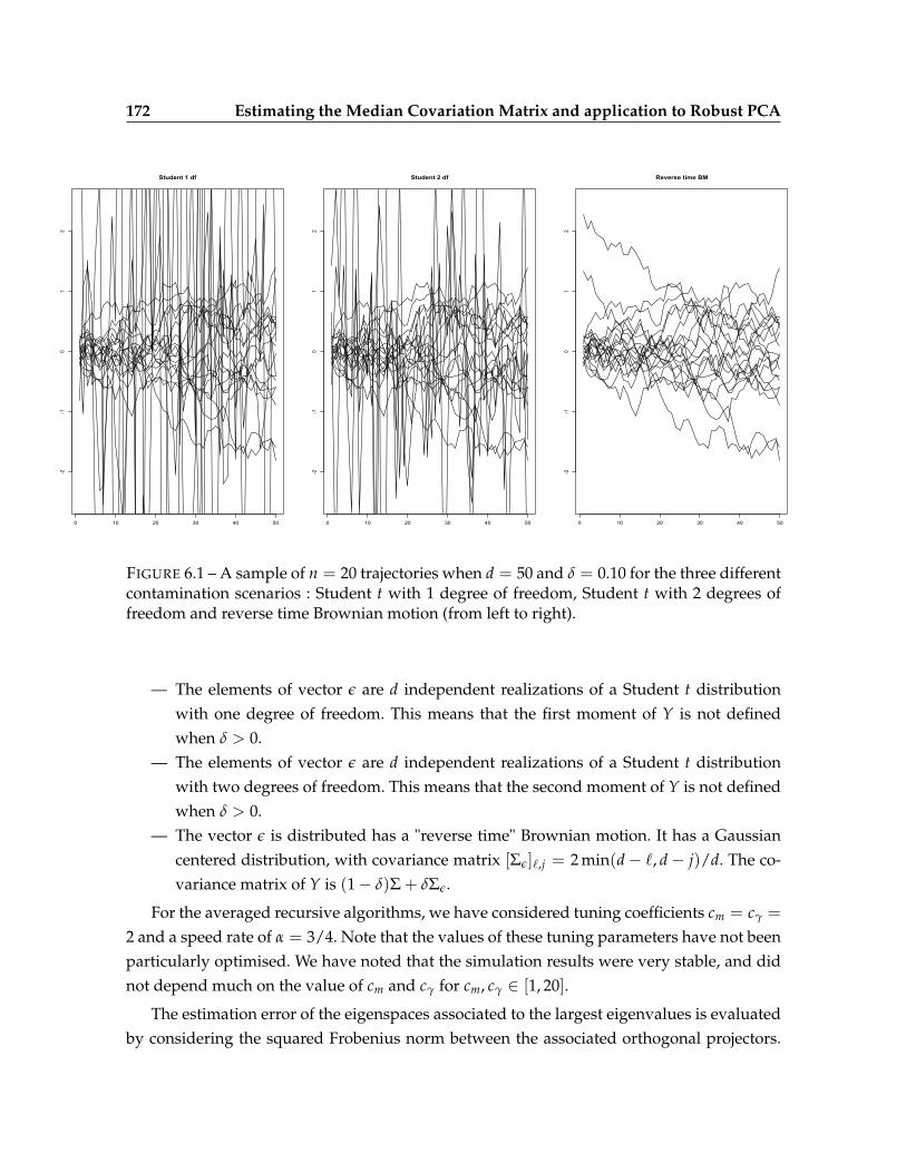
172 Estimating the Median Covariation Matrix and application to Robust PCA
0 10 20 30 40 50
-2-1
01
2
Student 1 df
0 10 20 30 40 50
-2-1
01
2
Student 2 df
0 10 20 30 40 50
-2-1
01
2
Reverse time BM
FIGURE 6.1 – A sample of n = 20 trajectories when d = 50 and δ = 0.10 for the three differentcontamination scenarios : Student t with 1 degree of freedom, Student t with 2 degrees offreedom and reverse time Brownian motion (from left to right).
— The elements of vector ε are d independent realizations of a Student t distributionwith one degree of freedom. This means that the first moment of Y is not definedwhen δ > 0.
— The elements of vector ε are d independent realizations of a Student t distributionwith two degrees of freedom. This means that the second moment of Y is not definedwhen δ > 0.
— The vector ε is distributed has a "reverse time" Brownian motion. It has a Gaussiancentered distribution, with covariance matrix [Σε]`,j = 2 min(d− `, d− j)/d. The co-variance matrix of Y is (1− δ)Σ + δΣε.
For the averaged recursive algorithms, we have considered tuning coefficients cm = cγ =
2 and a speed rate of α = 3/4. Note that the values of these tuning parameters have not beenparticularly optimised. We have noted that the simulation results were very stable, and didnot depend much on the value of cm and cγ for cm, cγ ∈ [1, 20].
The estimation error of the eigenspaces associated to the largest eigenvalues is evaluatedby considering the squared Frobenius norm between the associated orthogonal projectors.

6.4 An illustration on simulated and real data 173
Oracle MCD MCM(W) MCM(R) SphPCA PP PCA
0.005
0.020
0.050
0.200
0.500
2.000
FIGURE 6.2 – Estimation errors (at a logarithmic scale) over 200 Monte Carlo replications,for n = 200, d = 50 and a contamination by a t distribution with 2 degrees of freedomwith δ = 0.02. MCM(W) stands for the estimation performed by the Weiszfeld’s algorithmwhereas MCM(R) denotes the averaged recursive approach.
Denoting by Pq the orthogonal projector onto the space generated by the q eigenvectors ofthe covariance matrix Σ associated to the q largest eigenvalues and by Pq an estimation, weconsider the following loss criterion,
R(Pq, Pq) = tr[(
Pq − Pq
)T (Pq − Pq
)]= 2q− 2tr
[PqPq
]. (6.17)
Note that we always have R(Pq, Pq) ≤ 2q and R(Pq, Pq) = 2q means that the eigenspacesgenerated by the true and the estimated eigenvectors are orthogonal.

174 Estimating the Median Covariation Matrix and application to Robust PCA
t 1 df t 2 df inv. B. t 1 df t 2 df inv. B.δ Method d = 50 d = 200
0% PCA 0.015 0.0152% PCA 3.13 1.18 0.677 3.95 1.85 0.691
PP 0.097 0.087 0.090 0.099 0.088 0.093MCD 0.022 0.021 0.021 – – –Sph. PCA 0.029 0.028 0.029 0.031 0.027 0.028MCM (Weiszfeld) 0.021 0.021 0.022 0.023 0.021 0.021MCM (recursive) 0.023 0.024 0.025 0.026 0.023 0.026
5% PCA 3.82 1.91 0.884 3.96 1.98 0.925PP 0.100 0.099 0.096 0.097 0.091 0.098MCD 0.022 0.020 0.024 – – –Sph. PCA 0.029 0.029 0.033 0.030 0.029 0.038MCM (Weiszfeld) 0.022 0.021 0.029 0.023 0.023 0.033MCM (recursive) 0.026 0.024 0.033 0.027 0.026 0.038
10% PCA 3.83 1.95 1.05 3.96 1.99 1.12PP 0.107 0.109 0.099 0.100 0.105 0.093MCD 0.023 0.022 0.023 – – –Sph. PCA 0.031 0.031 0.059 0.030 0.028 0.056MCM (Weiszfeld) 0.024 0.023 0.059 0.022 0.023 0.056MCM (recursive) 0.030 0.027 0.072 0.028 0.026 0.069
20% PCA 3.84 2.02 1.19 3.96 2.01 1.25PP 0.114 0.132 0.134 0.084 0.115 0.132MCD 0.025 0.026 0.026 – – –Sph. PCA 0.038 0.036 0.140 0.033 0.035 0.155MCM (Weiszfeld) 0.030 0.029 0.167 0.025 0.026 0.184MCM (recursive) 0.040 0.035 0.211 0.035 0.031 0.224
TABLE 6.1 – Median estimation errors, according to criterion R(Pq, Pq) with a dimensionq = 2, for datasets with a sample size n = 200, over 500 Monte Carlo experiments.
6.4.2 Comparison with classical robust PCA techniques
We first compare the performances of the two estimators of the MCM based on the Weisz-feld’s algorithm and the recursive algorithms (see (6.14)) with more classical robust PCAtechniques.
We generated samples of Y with size n = 200 and dimension d ∈ 50, 200, over 500replications. Different levels of contamination are considered : δ ∈ 0, 0.02, 0.05, 0.10, 0.20.For both dimensions d = 50 and d = 200, the first eigenvalue of the covariance matrix of Xrepresents about 81 % of the total variance, and the second one about 9 %.
The median errors of estimation of the eigenspace generated by the first two eigenvectors(q = 2), according to criterion (6.17), are given in Table 6.1. In Figure 6.2, the distribution ofthe estimation error R(Pq, Pq) is drawn for the different approaches.
We can make the following remarks. At first note that even when the level of contami-

6.4 An illustration on simulated and real data 175
nation is small (2% and 5%), the performances of classical PCA are strongly affected by thepresence of outlying values in such (large) dimensions. When d = 50, the MCD algorithmand the MCM estimation provide the best estimations of the original two dimensional ei-genspace, whereas when d gets larger (d = n = 200), the MCD estimator can not be usedanymore (by construction) and the MCM estimator remains the most accurate. The perfor-mances of the spherical PCA are slightly less accurate whereas the median error of the robustPP is about four times larger. We can also note that the recursive MCM algorithm, which isdesigned to deal with very large samples, performs well even for such moderate samplesizes (see also Figure 6.2).
6.4.3 Online estimation of the principal components
We now consider an experiment in high dimension, d = 1000, and evaluate the abilityof the recursive algorithms defined in (6.15) to estimate recursively the eigenvectors of Γm
associated to the largest eigenvalues. Note that due to the high dimension of the data andlimited computation time, we only make comparison of the recursive robust techniques withthe classical PCA. For this we generate growing samples and compute, for each sample sizethe approximation error of the different (fast) strategies to the true eigenspace generated bythe q eigenvectors associated to the q largest eigenvalues of Γm.
We have drawn in Figure 6.3, the evolution of the mean (over 100 replications) approxi-mation error R(Pq, Pq), for a dimension q = 3, as a function of the sample size for samplescontaminated by a 2 degrees of freedom Student t distribution with a rate δ = 0.1. An impor-tant fact is that the recursive algorithm which approximates recursively the eigenelementsbehaves very well and we can see nearly no difference between the spectral decompositionof Vn (denoted by MCM in Figure 6.3) and the estimates produced with the sequential al-gorithm (6.15) for sample sizes larger than a few hundreds. We can also note that the errormade by the classical PCA is always very high and does not decrease with the sample size.
6.4.4 Robust PCA of TV audience
The last example is a high dimension and large sample case. Individual TV audiencesare measured, by the French company Médiamétrie, every minutes for a panel of n = 5422people over a period of 24 hours, d = 1440 (see [CCM12] for a more detailed presentation ofthe data). With a classical PCA, the first eigenspace represents 24.4% of the total variability,whereas the second one reproduces 13.5% of the total variance, the third one 9.64% and thefourth one 6.79%. Thus, more than 54% of the variability of the data can be captured in a fourdimensional space. Taking account of the large dimension of the data, these values indicate

176 Estimating the Median Covariation Matrix and application to Robust PCA
0 500 1000 1500 2000
0.00
50.
020
0.05
00.
200
0.50
02.
000
5.00
0
n
Est
imat
ion
erro
r (R
)
PCAOracleMCMMCM−update
FIGURE 6.3 – Estimation errors of the eigenspaces (criterion R(Pq)) with d = 1000 and q = 3for classical PCA, the oracle PCA and the recursive MCM estimator with recursive estima-tion of the eigenelements (MCM-update) and with static estimation (based on the spectraldecomposition of Vn) of the eigenelements (MCM).

6.4 An illustration on simulated and real data 177
0 200 400 600 800 1000 1200 1400
0.00
0.02
0.04
0.06
0.08
PC 1
minutes
PCAMCM
0 200 400 600 800 1000 1200 1400
-0.06
-0.04
-0.02
0.00
0.02
0.04
0.06
PC 2
minutes
TV
aud
ienc
e
PCAMCM
FIGURE 6.4 – TV audience data measured the 6th September 2010, at the minute scale. Com-parison of the principal components of the classical PCA (black) and robust PCA based onthe Median Covariation Matrix (red). First eigenvectors on the left, second eigenvectors onthe right.
a high temporal correlation.
Because of the large dimension of the data, the Weiszfeld’s algorithm as well as the otherrobust PCA techniques can not be used anymore in reasonable time with a personal com-puter. The MCM has been computed thanks to the recursive algorithm given in (6.14) inapproximately 3 minutes on a laptop in the R language (without any specific C routine).
As seen in Figure 6.4, the first two eigenvectors obtained by a classical PCA and the ro-bust PCA based on the MCM are rather different. This is confirmed by the relatively largedistance between the two corresponding eigenspaces, R(PPCA
2 , PMCM2 ) = 0.56. The first ro-
bust eigenvector puts the stress on the time period comprised between 1000 minutes and1200 minutes whereas the first non robust eigenvector focuses, with a smaller intensity, on alarger period of time comprised between 600 and 1200 minutes. The second robust eigenvec-tor differentiates between people watching TV during the period between 890 and 1050 mi-nutes (negative value of the second principal component) and people watching TV between

178 Estimating the Median Covariation Matrix and application to Robust PCA
0 200 400 600 800 1000 1200 1400
-0.04
-0.02
0.00
0.02
0.04
0.06
0.08
PC 3
minutes
PCAMCM
0 200 400 600 800 1000 1200 1400
-0.06
-0.04
-0.02
0.00
0.02
0.04
0.06
PC 4
minutes
TV a
udie
nce
PCAMCM
FIGURE 6.5 – TV audience data measured the 6th September 2010, at the minute scale. Com-parison of the principal components of the classical PCA (black) and robust PCA based onthe MCM (red). Third eigenvectors on the left, fourth eigenvectors on the right.
minutes 1090 and 1220 (positive value of the second principal component). Rather surprisin-gly, the third and fourth eigenvectors of the non robust and robust covariance matrices lookquite similar (see Figure 6.5).
6.5 Proofs
We give in this Section the proofs of Theorems 6.3.2, 6.3.3 and 6.3.4. These proofs rely onseveral technical Lemmas whose proofs are given in the Supplementary file.

6.5 Proofs 179
6.5.1 Proof of Theorem 6.3.2
Let us recall the Robbins-Monro algorithm, defined recursively by
Vn+1 = Vn + γn(Xn+1 −mn) (Xn+1 −mn)
T −Vn∥∥∥(Xn+1 −mn) (Xn+1 −mn)T −Vn
∥∥∥F
= Vn − γnUn+1,
with Un+1 := − (Xn+1−mn)(Xn+1−mn)T−Vn
‖(Xn+1−mn)(Xn+1−mn)T−Vn‖F
. Since Fn := σ (X1, ..., Xn), we have E [Un+1|Fn] =
∇Gmn(Vn). Thus ξn+1 := ∇mn G(Vn) − Un+1, (ξn) is a sequence of martingale differencesadapted to the filtration (Fn). Indeed, E [ξn+1|Fn] = ∇Gmn(Vn) − E [Un+1|Fn] = 0. Thealgorithm can be written as follows
Vn+1 = Vn − γn∇Gmn(Vn) + γnξn+1.
Moreover, it can be considered as a stochastic gradient algorithm because it can be decom-posed as follows :
Vn+1 = Vn − γn (∇Gmn(Vn)−∇Gmn(Γm)) + γnξn+1 − γnrn, (6.18)
with rn := ∇Gmn(Γm)−∇Gm(Γm). Finally, linearizing the gradient,
Vn+1 − Γm =(
IS(H) − γn∇2mG(Γm)
)(Vn − Γm) + γnξn+1 − γnrn − γnr′n − γnδn, (6.19)
with
r′n :=(∇2
mnG (Γm)−∇2
mG (Γm))(Vn − Γm) ,
δn := ∇Gmn (Vn)−∇Gmn (Γm)−∇2mn
G (Γm) (Vn − Γm) .
The following lemma gives upper bounds of these remainder terms. Its proof is given inthe Supplementary file.
Lemma 6.5.1. Under assumptions 1-3(b), we can bound the three remainder terms. First,
‖δn‖F ≤ 6C ‖Vn − Γm‖2F . (6.20)

180 Estimating the Median Covariation Matrix and application to Robust PCA
In the same way, for all n ≥ 1,
‖rn‖F ≤ 4(√
C + C√‖Γm‖F
)‖mn −m‖ . (6.21)
Finally, for all n ≥ 1,
∥∥r′n∥∥
F ≤ 12(
C√‖Γm‖F + C3/4
)‖mn −m‖ ‖Vn − Γm‖F . (6.22)
We deduce from decomposition (6.18) that for all n ≥ 1,
‖Vn+1 − Γm‖2F = ‖Vn − Γm‖2
F − 2γn 〈Vn − Γm,∇Gmn(Vn)−∇Gmn(Γm)〉F+ γ2
n ‖∇Gmn(Vn)−∇Gmn(Γm)‖2F
+ γ2n ‖ξn+1‖2
F + 2γn 〈Vn − Γm − γn (∇Gmn(Vn)−∇Gmn(Γm)) , ξn+1〉F+ γ2
n ‖rn‖2F − 2γn 〈rn, Vn − Γm〉F − 2γ2
n 〈rn, ξn+1 −∇Gmn(Vn) +∇Gmn(Γm)〉F .
Note that for all h ∈ H and V ∈ S(H) we have ‖∇Gh(V)‖F ≤ 1. Furthermore, ‖rn‖F ≤ 2and ‖ξn+1‖F ≤ 2. Using the fact that (ξn) is a sequence of martingale differences adapted tothe filtration (Fn),
E[‖Vn+1 − Γm‖2
F |Fn
]≤ ‖Vn − Γm‖2
F − 2γn 〈Vn − Γm,∇mn G (Vn)−∇mn G (Γm)〉F+ 28γ2
n − 2γn 〈rn, Vn − Γm〉F .
Let αn = n−β, with β ∈ (1− α, α), we have
E[‖Vn+1 − Γm‖2
F |Fn
]≤ (1 + γnαn) ‖Vn − Γm‖2
F − 2γn 〈Vn − Γm,∇mn G (Vn)−∇mn G (Γm)〉F(6.23)
+ 28γ2n +
γn
αn‖rn‖2
F .
Moreover, applying Lemma 6.5.1 and Theorem 5.1 in [GB15], we get for all positiveconstant δ,
‖rn‖2F = O
(‖mn −m‖2
)= O
((ln n)1+δ
n
)a.s.
Thus, since 2γn 〈Vn − Γm,∇mn G (Vn)−∇mn G (Γm)〉F ≥ 0, the Robbins-Siegmund Theorem(see [Duf97] for instance) ensures that ‖Vn − Γm‖F converges almost surely to a finite random

6.5 Proofs 181
variable and
∑n≥1
γn 〈Vn − Γm,∇mn G (Vn)−∇mn G (Γm)〉F < +∞ a.s.
Furthermore, by induction, inequality (6.23) becomes
E[‖Vn+1 − Γm‖2
F
]≤(
∞
∏k=1
(1 + γkαk)
)E[‖V1 − Γm‖2
F
]+ 28
(∞
∏k=1
(1 + γkαk)
)∞
∑k=1
γ2k
+
(∞
∏k=1
(1 + γkαk)
)∞
∑k=1
γk
αkE[‖rk‖2
F
].
Since β < α, applying Theorem 4.2 in [GB15] and Lemma 6.1, there is a positive constant C0
such that∞
∑k=1
γk
αkE[‖rk‖2
F
]= C0
∞
∑k=1
k−α−1−β < +∞.
Thus, there is a positive constant M such that for all n ≥ 1, E[‖Vn − Γm‖2
F
]≤ M. Since mn
converges almost surely to m, one can conclude the proof of the almost sure consistency ofVn with the same arguments as in the proof of Theorem 3.1 in [CCZ13] and the convexityproperties given in the Section B of the supplementary file.
Finally, the almost sure consistency of Vn is obtained by a direct application of Topelitz’slemma (see e.g. Lemma 2.2.13 in [Duf97]).
6.5.2 Proof of Theorem 6.3.3
The proof of Theorem 6.3.3 relies on properties of the p-th moments of Vn for all p ≥1 given in the following three Lemmas. These properties enable us, with the applicationof Markov’s inequality, to control the probability of the deviations of the Robbins Monroalgorithm from Γm.
Lemma 6.5.2. Under assumptions 1-3(b), for all integer p, there is a positive constant Mp such thatfor all n ≥ 1,
E[‖Vn − Γm‖2p
F
]≤ Mp.
Lemma 6.5.3. Under assumptions 1-3(b), there are positive constants C1, C′1, C2, C3 such that for alln ≥ 1,
E[‖Vn − Γm‖2
]≤ C1e−C′1n1−α
+C2
nα+ C3 sup
E(n/2)+1≤k≤n−1E[‖Vk − Γm‖4
],

182 Estimating the Median Covariation Matrix and application to Robust PCA
where E(x) is the integer part of the real number x.
Lemma 6.5.4. Under assumptions 1-3(b), for all integer p′ ≥ 1, there are a rank np′ and positiveconstants C1,p′ , C2,p′ , C3,p′ , cp′ such that for all n ≥ np′ ,
E[‖Vn+1 − Γm‖4
F
]≤(
1− cp′γnn−1−α
p′
)E[‖Vn − Γm‖4
F
]+
C1,p′
n3α+
C2,p′
n2αE[‖Vn − Γm‖2
F
]+
C3,p′
n3α−3 1−αp′
.
We can now prove Theorem 6.3.3.
Let us choose an integer p′ such that p′ > 3/2. Thus, 2 + α − 3 1−αp′ ≥ 3α, and
applying Lemma 6.5.4, there are positive constants C1,p′ , C2,p′ , cp′ and a rank np′ such that forall n ≥ np′ ,
E[‖Vn+1 − Γm‖4
F
]≤(
1− cp′γnn−1−α
p′
)E[‖Vn − Γm‖4
F
]+
C1,p′
n3α+
C2,p′
n2αE[‖Vn − Γm‖2
F
].
(6.24)
Let us now choose β ∈ (α, 2α) and p′ such that p′ > 1−α2α−β . Note that 3α− β > α + 1−α
p′ .One can check that there is a rank n′p′ ≥ np′ such that for all n ≥ n′p′ ,
(n + 1)αC1e−C′1n1−α+
12+ C32β+1 1
(n + 1)β−α≤ 1,(
1− cp′γnn−1−α
p′
)(n + 1
n
)β
+ 23α C1,p′ + C2,p′
(n + 1)3α−β≤ 1.
With the help of a strong induction, we are going to prove the announced results, that is tosay that there are positive constants Cp′ , Cβ such that 2Cp′ ≥ Cβ ≥ Cp′ ≥ 1 and Cp′ ≥ 2α+1C2
(with C2 defined in Lemma 6.5.3), such that for all n ≥ 1,
E[‖Vn − Γm‖2
F
]≤
Cp′
nα,
E[‖Vn − Γm‖4
F
]≤
Cβ
nβ.
First, let us choose Cp′ and Cβ such that
Cp′ ≥ maxk≤n′p′
kαE
[‖Vk − Γm‖2
F
],
Cβ ≥ maxk≤n′p′
kβE
[∥∥∥Vn′p′− Γm
∥∥∥4
F
].

6.5 Proofs 183
Thus, for all k ≤ n′p′ ,
E[‖Vk − Γm‖2
F
]≤
Cp′
kα,
E[‖Vk − Γm‖4
F
]≤
Cβ
kβ.
We suppose from now that n ≥ n′p′ and that previous inequalities are verified for all k ≤n− 1. Applying Lemma 6.5.2 and by induction,
E[‖Vn+1 − Γm‖2
F
]≤ C1e−C′1n1−α
+C2
nα+ C3 sup
E((n+1)/2)+1≤k≤n
E[‖Vk − Γm‖4
F
]≤ C1e−C′1n1−α
+C2
nα+ C3 sup
E((n+1)/2)+1≤k≤n
Cβ
kβ
≤ C1e−C′1n1−α
+C2
nα+ C32β Cβ
nβ.
Since 2Cp′ ≥ Cβ ≥ Cp′ ≥ 1 and since Cp′ ≥ 2α+1C2, factorizing byCp′
(n+1)α ,
E[‖Vn+1 − Γm‖2
F
]≤ Cp′C1e−C′1n1−α
+ Cp′2−α−1 1nα
+ C32β 2Cp′
nβ
≤C′p
(n + 1)α(n + 1)αC1e−C′1n1−α
+ 2−α
(n
n + 1
)α Cp′
2(n + 1)α+
C32β+1
(n + 1)β−α
Cp′
(n + 1)α
≤C′p
(n + 1)αC1(n + 1)αe−C′1n1−α
+12
Cp′
(n + 1)α+ C32β+1 1
(n + 1)β−α
Cp′
(n + 1)α
≤((n + 1)αC1e−C′1n1−α
+12+ C32β+1 1
(n + 1)β−α
)Cp′
(n + 1)α.
By definition of n′p′ ,
E[‖Vn+1 − Γm‖2
F
]≤
Cp′
(n + 1)α. (6.25)
In the same way, applying Lemma 6.5.4 and by induction,
E[‖Vn+1 − Γm‖4
F
]≤(
1− cp′γnn−1−α
p′
)E[‖Vn − Γm‖4
F
]+
C1,p′
n3α+
C2,p′
n2αE[‖Vn − Γm‖2
F
]≤(
1− cp′γnn−1−α
p′
)Cβ
nβ+
C1,p′
n3α+
C2,p′
n2α
Cp′
nα.

184 Estimating the Median Covariation Matrix and application to Robust PCA
Since Cβ ≥ Cp′ ≥ 1, factorizing by Cβ
(n+1)β ,
E[‖Vn+1 − Γm‖4
F
]≤(
1− cp′γnn−1−α
p′
)Cβ
nβ+(C1,p′ + C2,p′
) Cβ
n3α
≤(
1− cp′γnn−1−α
p′
)(n + 1
n
)β Cβ
nβ+ 23α C1,p′ + C2,p′
(n + 1)3α−β
Cβ
(n + 1)β
≤((
1− cp′γnn−1−α
p′
)(n + 1
n
)β
+ 23α C1,p′ + C2,p′
(n + 1)3α−β
)Cβ
(n + 1)β.
By definition of n′p′ ,
E[‖Vn+1 − Γm‖4
F
]≤
Cβ
(n + 1)β, (6.26)
which concludes the induction and the proof.
6.5.3 Proof of Theorem 6.3.4
In order to prove Theorem 6.3.4, we first recall the following Lemma.
Lemma 6.5.5 ([GB15]). Let Y1, ..., Yn be random variables taking values in a normed vector spacesuch that for all positive constant q and for all k ≥ 1, E
[‖Yk‖q] < ∞. Then, for all real numbers
a1, ..., an and for all integer p, we have
E
[∥∥∥∥∥ n
∑k=1
akYk
∥∥∥∥∥p]≤(
n
∑k=1|ak|
(E[‖Yk‖p]) 1
p
)p
(6.27)
We can now prove Theorem 6.3.4. Let us rewrite decomposition (6.19) as follows
∇2mG (Γm) (Vn − Γm) =
Tn
γn− Tn+1
γn+ ξn+1 − rn − r′n − δn, (6.28)
with Tn := Vn − Γm. As in [Pel00], we sum these equalities, apply Abel’s transform anddivide by n to get
∇2mG (Γm)
(Vn − Γm
)=
1n
(T1
γ1− Tn+1
γn+1+
n
∑k=2
Tk
(1γk− 1
γk−1
)−
n
∑k=1
δk −n
∑k=1
rk −n
∑k=1
r′k +n
∑k=1
ξk+1
).
We now bound the quadratic mean of each term at the right-hand side of previous equality.

6.5 Proofs 185
First, we have 1n2 E
[∥∥∥ T1γ1
∥∥∥2
F
]= o
( 1n
). Applying Theorem 6.3.3,
1n2 E
[∥∥∥∥Tn+1
γn
∥∥∥∥2
F
]≤ 1
n2
C′c−2γ
n−α= o
(1n
).
Moreover, since∣∣∣γ−1
k − γ−1k−1
∣∣∣ ≤ 2αc−1γ kα−1, the application of Lemma 6.5.5 and Theorem 6.3.3
gives
1n2 E
∥∥∥∥∥ n
∑k=2
(γ−1
k − γ−1k−1
)Tk
∥∥∥∥∥2
F
≤ 1n2
(n
∑k=2
∣∣∣γ−1k − γ−1
k−1
∣∣∣√E[‖Tk‖2
F
])2
≤ 1n2 4α2c−2
γ C′(
n
∑k=2
1k1−α/2
)2
= O(
1n2−α
)= o
(1n
),
since α < 1. In the same way, since ‖δn‖F ≤ 6C ‖Tn‖2F, applying Lemma 6.5.5 and Theo-
rem 6.3.3 with β > 1,
1n2 E
∥∥∥∥∥ n
∑k=1
δk
∥∥∥∥∥2
F
≤ 1n2
(n
∑k=1
√E[‖δk‖2
F
])2
≤ 36C2
n2
(n
∑k=1
√E[‖Tk‖4
F
])2
≤36C2Cβ
n2
(n
∑k=1
1kβ/2
)2
= O(
1nβ
)= o
(1n
),
Moreover, let D := 12(√
C + C√‖Γm‖F
). Since ‖rn‖F ≤ D ‖mn −m‖, and since there is a
186 Estimating the Median Covariation Matrix and application to Robust PCA
positive constant C′′ such that for all n ≥ 1, E[‖mn −m‖2
]≤ C′′n−1,
1n2 E
∥∥∥∥∥ n
∑k=1
rk
∥∥∥∥∥2
F
≤ 1n2
(n
∑k=1
√E[‖rk‖2
F
])2
≤ D2
n2
(n
∑k=1
√E[‖mn −m‖2
])
≤ D2C′′
n2
(n
∑k=1
1k1/2
)2
= O(
1n
).
Since ‖r′n‖F ≤ C0 ‖mn −m‖ ‖Vn − Γm‖2F with C0 := 12
(C√‖Γm‖F + C3/4), Cauchy-Schwarz’s
inequality and Lemma 6.5.5 give
1n2 E
∥∥∥∥∥ n
∑k=1
r′n
∥∥∥∥∥2
F
≤ 1n2
(n
∑k=1
√E[‖r′n‖
2F
])2
≤ C20
n2
(n
∑k=1
√E[‖mn −m‖2 ‖Vn − Γm‖2
F
])2
≤ C20
n2
(n
∑k=1
(E[‖mn −m‖4
]) 14(
E[‖Vn − Γm‖4
F
]) 14
)2
.
Applying Theorem 4.2 in [GB15] and Theorem 3.3,
1n2 E
∥∥∥∥∥ n
∑k=1
r′n
∥∥∥∥∥2
F
≤ C20√
Cβ
√K2
n2
(n
∑k=1
1kβ/4+1/2
)2
= O(
1n1+β/2
)= o
(1n
),
since β > 0. Finally, one can easily check that E[‖ξn+1‖2
F
]≤ 1, and since (ξn) is a sequence

6.6 Concluding remarks 187
of martingale differences adapted to the filtration (Fn),
1n2 E
∥∥∥∥∥ n
∑k=1
ξk+1
∥∥∥∥∥2
F
=1n2
(n
∑k=1
E[‖ξk+1‖2
F
]+ 2
n
∑k=1
n
∑k′=k+1
E [〈ξk+1, ξk′+1〉F])
=1n2
(n
∑k=1
E[‖ξk+1‖2
F
]+ 2
n
∑k=1
n
∑k′=k+1
E[⟨
ξk+1, E[ξk′+1
∣∣∣Fk′]⟩
F
])
=1n2
n
∑k=1
E[‖ξk+1‖2
F
]≤ 1
n.
Thus, there is a positive constant K such that for all n ≥ 1,
E[∥∥∇2
mG (Γm)(Vn − Γm
)∥∥2F
]≤ K
n.
Let λmin be the smallest eigenvalue of ∇2mG (Γm). We have, with Proposition B.1 in the sup-
plementary file, that λmin > 0 and the announced result is proven,
E[∥∥Vn − Γm
∥∥2F
]≤ K
λ2minn
.
6.6 Concluding remarks
The simulation study and the illustration on real data indicate that performing robustprincipal components analysis via the median covariation matrix, which can bring new in-formation compared to classical PCA, is an interesting alternative to more classical robustprincipal components analysis techniques. The use of recursive algorithms permits to per-form robust PCA on very large datasets, in which outlying observations may be hard todetect. Another interest of the use of such sequential algorithms is that estimation of the me-dian covariation matrix as well as the principal components can be performed online withautomatic update at each new observation and without being obliged to store all the data inmemory.
A deeper study of the asymptotic behaviour of the recursive algorithms would certainlydeserve further investigations. Proving the asymptotic normality and obtaining the limitingvariance of the sequence of estimators Vn when m is unknown would be of great interest.It a challenging issue that is beyond the scope of the paper and would require to study thejoint weak convergence of the two simultaneous recursive averaged estimators of m and Γm.

188 Estimating the Median Covariation Matrix and application to Robust PCA
The use of the MCM could be interesting to robustify the estimation in many differentstatistical models, particularly with functional data. For example, it could be employed as analternative to robust functional projection pursuit in robust functional time series predictionor for robust estimation in functional linear regression, with the introduction of the mediancross-covariation matrix.
Acknowledgements. We thank the company Médiamétrie for allowing us to illustrate ourmethodologies with their data. We also thank Dr. Peggy Cénac for a careful reading of theproofs.
Annexe C
Fast Estimation of the MedianCovariation Matrix with Applicationto Online Robust PrincipalComponents Analysis. Appendix
Résumé
Dans cette partie, nous commençons par rappeler comment estimer la médiane géomé-trique et la Median Covariation Matrix à l’aide de l’algorithme de Weiszfeld. Ensuite, nousdonnons des propriétés de convexité de la fonction que l’on veut minimiser, avant de rappe-ler quelques décompositions des algorithmes. Enfin, les preuves des lemmes et propositionstechniques sont données. Plus précisément, on donne la preuve du Lemme 6.5.1, qui per-met de majorer les termes de reste. De plus, on prouve les Lemmes 6.5.2, 6.5.3 et 6.5.4 quipermettent d’obtenir la vitesse de convergence en moyenne quadratique de l’algorithme degradient stochastique.

190 Estimating the Median Covariation Matrix. Appendix
C.1 Estimating the median covariation matrix with Weiszfeld’s al-gorithm
Suppose we have a fixed size sample X1, . . . , Xn and we want to estimate the geometricmedian.
The iterative Weiszfeld’s algorithm relies on the fact that the solution m∗n of the followingoptimization problem
minµ∈H
n
∑i=1‖Xi − µ‖
satisfies, when m∗n 6= Xi, for all i = 1, . . . , n
m∗n =n
∑i=1
wi (m∗n) Xi
where the weights wi(x) are defined by
wi(x) =‖Xi − x‖−1
n
∑j=1
∥∥Xj − x∥∥−1
.
Weiszfeld’s algorithm is based on the following iterative scheme. Consider first a pilotestimator m(0) of m. At step (e), a new approximation m(e+1)
n to m is given by
m(e+1)n =
n
∑i=1
wi
(m(e)
n
)Xi. (C.1)
The iterative procedure is stopped when∥∥∥m(e+1)
n − m(e)n
∥∥∥ ≤ ε, for some precision ε known inadvance. The final value of the algorithm is denoted by mn.
The estimator of the MCM is computed similarly. Suppose Γ(e) has been calculated at step(e), then at step (e + 1), the new approximation Γ(e+1) to Γm is defined by
Γ(e+1)n =
n
∑i=1
Wi
(Γ(e))(Xi − mn)(Xi − mn)
T. (C.2)
The procedure is stopped when∥∥∥Γ(e+1) − Γ(e)
∥∥∥F≤ ε, for some precision ε fixed in advance.
Note that by construction, this algorithm leads to an estimated median covariation matrixthat is always non negative.

C.2 Convexity results 191
C.2 Convexity results
In this section, we first give and recall some convexity properties of functional Gh. Thefollowing one gives some information on the spectrum of the Hessian of G.
Proposition C.2.1. Under assumptions 1-3(b), for all h ∈ H and V ∈ S(H), S(H) admits anorthonormal basis composed of eigenvectors of ∇2
hG(V). Let us denote by λh,V,i, i ∈N the set ofeigenvalues of ∇2
hG(V). For all i ∈N,
0 ≤ λh,V,i ≤ C.
Moreover, there is a positive constant cm such that for all i ∈N,
0 < cm ≤ λm,Γm,i ≤ C.
Finally, by continuity, there are positive constants ε, ε′ such that for all h ∈ B (m, ε) andV ∈ B (Γm, ε′), and for all i ∈N,
12
cm ≤ λh,V,i ≤ C.
The proof is very similar to the one in [CCZ13] and consequently it is not given here.Furthermore, as in [CCGB15], it ensures the local strong convexity as shown in the followingcorollary.
Corollary C.2.1. Under assumptions 1-3(b), for all positive constant A, there is a positive constantcA such that for all V ∈ B (Γm, A) and h ∈ B (m, ε),
〈∇hG(V)−∇hG(Γm), V − Γm〉H ≥ cA ‖V − Γm‖2F .
Finally, the following lemma gives an upper bound on the remainder term in the Taylor’sexpansion of the gradient.
Lemma C.2.1. Under assumptions 1-3(b), for all h ∈ H and V ∈ S(H),
∥∥∇Gh(V)−∇Gh (Γm)−∇2hG (Γm) (V − Γm)
∥∥F ≤ 6C ‖V − Γm‖2
F . (C.3)
Proof of Lemma C.2.1. Let δV,h := ∇Gh(V)−∇Gh (Γm)−∇2hG (Γm) (V − Γm), since

192 Estimating the Median Covariation Matrix. Appendix
∇Gh(V) − ∇Gh (Γm) =∫ 1
0 ∇2hG (Γm + t (V − Γm)) (V − Γm) dt, we have
‖δV,h‖F =
∥∥∥∥∫ 1
0∇2
hG (Γm + t (V − Γm)) ((V − Γm) dt−∇2hG (Γm) (V − Γm)
∥∥∥∥F
≤∫ 1
0
∥∥∇2hG (Γm + t (V − Γm)) ((V − Γm)−∇2
hG (Γm) (V − Γm)∥∥
F dt.
As in the proof of Lemma 5.1 in [CCGB15], under assumptions 1-3(b), one can check that forall h ∈ H, and t ∈ [0, 1],
∥∥∇2hG (Γm + t (V − Γm)) ((V − Γm)−∇2
hG (Γm) (V − Γm)∥∥
F ≤ 6C ‖V − Γm‖2F ,
which concludes the proof.
C.3 Decompositions of the Robbins-Monro algorithm and proof ofLemma 6.5.1
Let us recall that the Robbins-Monro algorithm is defined recursively by
Vn+1 = Vn + γn(Xn+1 −mn) (Xn+1 −mn)
T −Vn∥∥∥(Xn+1 −mn) (Xn+1 −mn)T −Vn
∥∥∥F
= Vn − γnUn+1,
with Un+1 := − (Xn+1−mn)(Xn+1−mn)T−Vn
‖(Xn+1−mn)(Xn+1−mn)T−Vn‖F
. Let us remark that ξn+1 := ∇mn G(Vn) − Un+1,
(ξn) is a sequence of martingale differences adapted to the filtration (Fn) and the algorithmcan be written as follows
Vn+1 = Vn − γn (∇Gmn(Vn)−∇Gmn(Γm)) + γnξn+1 − γnrn, (C.4)
with rn := ∇Gmn(Γm)−∇Gm(Γm). Finally, let is consider the following linearization of thegradient,
Vn+1 − Γm =(
IS(H) − γn∇2mG(Γm)
)(Vn − Γm) + γnξn+1 − γnrn − γnr′n − γnδn, (C.5)

C.3 Return on the RM algorithm and proof of Lemma 6.5.1 193
with
r′n :=(∇2
mnG (Γm)−∇2
mG (Γm))(Vn − Γm) ,
δn := ∇Gmn (Vn)−∇Gmn (Γm)−∇2mn
G (Γm) (Vn − Γm) .
Proof of Lemma 6.5.1. The bound of ‖δn‖ is a corollary of Lemma C.2.1.
Bounding ‖rn‖
Let us recall that for all h ∈ H, Y(h) := (X− h) (X− h)T. We now define for all h ∈ Hthe random function ϕh : [0, 1] −→ S(H) defined for all t ∈ [0, 1] by
ϕh(t) :=Y(m + th)− Γm
‖Y(m + th)− Γm‖F.
Note that rn = E[
ϕmn−m(0)− ϕmn−m(1)∣∣∣Fn
]. Thus, by dominated convergence,
‖rn‖F ≤ supt∈[0,1]
E[∥∥ϕ′mn−m(t)
∥∥F
∣∣∣Fn
].
Moreover, one can check that for all h ∈ H,
ϕ′h(t) = −h (X−m− th)T
‖Y(m + th)− Γm‖F− (X−m− th) hT
‖Y(m + th)− Γm‖F
+⟨
Y(m + th)− Γm, h (X−m− th)T⟩
F
Y(m + th)− Γm
‖Y(m + th)− Γm‖3F
+⟨
Y(m + th)− Γm, (X−m− th) hT⟩
F
Y(m + th)− Γm
‖Y(m + th)− Γm‖3F
.
We now bound each term on the right-hand side of previous equality. First, applying Cauchy-Schwarz’s inequality and using the fact that for all h, h′ ∈ H,
∥∥hh′T∥∥
F = ‖h‖ ‖h′‖,
E
∥∥∥h (X−m− th)T
∥∥∥F
‖Y(m + th)− Γm‖F
≤ ‖h‖E
[‖X−m− th‖
‖Y(m + th)− Γm‖F
]
≤ ‖h‖E
[ √‖Y(m + th)‖F
‖Y(m + th)− Γm‖F
]
≤ ‖h‖(
E
[ √‖Γm‖F
‖Y(m + th)− Γm‖F
]+ E
[1√
‖Y(m + th)− Γm‖F
]).

194 Estimating the Median Covariation Matrix. Appendix
Thus, since E[
1‖Y(m+th)−Γm‖F
]≤ C,
E
∥∥∥h (X−m− th)T
∥∥∥F
‖Y(m + th)− Γm‖F
≤ ‖h‖(C√‖Γm‖F +
√C)
. (C.6)
In the same way,
E
[∥∥(X−m− th) hT∥∥
F‖Y(m + th)− Γm‖F
]≤ ‖h‖
(C√‖Γm‖F +
√C)
. (C.7)
Applying Cauchy-Schwarz’s inequality,
E
[∣∣∣⟨Y(m + th)− Γm, h (X−m− th)T⟩
F
∣∣∣ ‖Y(m + th)− Γm‖F
‖Y(m + th)− Γm‖3F
]≤ E
∥∥∥h (X−m− th)T
∥∥∥F
‖Y(m + th)− Γm‖F
≤ ‖h‖E
[‖X−m− th‖
‖Y(m + th)− Γm‖F
]≤ ‖h‖E
[ √‖Y(m + th)‖F
‖Y(m + th)− Γm‖F
].
Thus, since E[
1‖Y(m+th)−Γm‖F
]≤ C, and since for all positive constants a, b,
√a + b ≤
√a +√
b,
‖h‖E
[ √‖Y(m + th)‖F
‖Y(m + th)− Γm‖F
]≤ ‖h‖
(E
[ √‖Γm‖F
‖Y(m + th)− Γm‖F
]+ E
[1√
‖Y(m + th)− Γm‖F
])
≤ ‖h‖(
C√‖Γm‖F +
√C)
.
Finally,
E
[∣∣∣⟨Y(m + th)− Γm, h (X−m− th)T⟩
F
∣∣∣ ‖Y(m + th)− Γm‖F
‖Y(m + th)− Γm‖3F
]≤ ‖h‖
(C√‖Γm‖F +
√C)
,
(C.8)
E
[∣∣∣⟨Y(m + th)− Γm, (X−m− th) hT⟩
F
∣∣∣ ‖Y(m + th)− Γm‖F
‖Y(m + th)− Γm‖3F
]≤ ‖h‖
(C√‖Γm‖F +
√C)
.
(C.9)

C.3 Return on the RM algorithm and proof of Lemma 6.5.1 195
Applying inequalities (C.6) to (C.9) with h = mn −m, the announced result is proven,
‖rn‖F ≤ 4(√
C + C√‖Γm‖F
)‖mn −m‖ .
Bounding ‖r′n‖For all h ∈ H and V ∈ S(H), we define the random function ϕh,V : [0, 1] −→ S(H)
such that for all t ∈ [0, 1],
ϕh,V(t) :=1
‖Y(m + th)− Γm‖F
(IS(H) −
(Y(m + th)− Γm)⊗F (Y(m + th)− Γm)
‖Y(m + th)− Γm‖2F
)(V) .
Note that r′n = E[
ϕmn−m,Vn−Γm(1)− ϕmn−m,Vn−Γm(0)∣∣∣Fn
]. By dominated convergence,
∥∥r′n∥∥
F ≤ supt∈[0,1]
E[∥∥ϕ′mn−m,Vn−Γm
(t)∥∥
F
∣∣∣Fn
].
Moreover, as for the bound of ‖rn‖, one can check, with an application of Cauchy-Schwarz’sinequality, that for all h ∈ H, V ∈ S(H), and t ∈ [0, 1],
ϕ′h,V(t) ≤ 6‖Y(m + th)− Γm‖F
∥∥hT(X−m− th)∥∥
F
‖Y(m + th)− Γm‖3F
‖V‖F
+ 6‖Y(m + th)− Γm‖F
∥∥h(X−m− th)T∥∥
F
‖Y(m + th)− Γm‖5F
‖(Y(m + th)− Γm)⊗F (Y(m + th)− Γm) (V)‖F
≤ 12
∥∥h(X−m− th)T∥∥
F
‖Y(m + th)− Γm‖2F
‖V‖F .
Finally,
E
[∥∥h(X−m− th)T∥∥
F
‖Y(m + th)− Γm‖2F
‖V‖F
]≤ E
[‖h‖ ‖X−m− th‖‖Y(m + th)− Γm‖2
F
‖V‖F
]
≤ ‖h‖ ‖V‖F E
[ √‖Γm‖F
‖Y(m + th)− Γm‖2F
]
+ ‖h‖ ‖V‖F E
[1
‖Y(m + th)− Γm‖3/2F
]
≤(
C√‖Γm‖F + C3/4
)‖h‖ ‖V‖F . (C.10)
Then the announced result follows from an application of inequality (C.10) with h = mn −m

196 Estimating the Median Covariation Matrix. Appendix
and V = Vn − Γm,
∥∥r′n∥∥ ≤ 12
(C√‖Γm‖F + C3/4
)‖mn −m‖ ‖Vn − Γm‖F .
C.4 Proofs of Lemma 6.5.2, 6.5.3 and 6.5.4
Proof of Lemma 6.5.2. Using decomposition (C.4),
‖Vn+1 − Γm‖2F = ‖Vn − Γm‖2
F − 2γn 〈Vn − Γm,∇Gmn(Vn)−∇Gmn(Γm)〉F+ γ2
n ‖∇Gmn(Vn)−∇Gmn(Γm)‖2F
+ γ2n ‖ξn+1‖2
F + 2γn 〈Vn − Γm − γn (∇Gmn(Vn)−∇Gmn(Γm)) , ξn+1〉F+ γ2
n ‖rn‖2F − 2γn 〈rn, Vn − Γm〉F − 2γ2
n 〈rn, ξn+1 −∇Gmn(Vn) +∇Gmn(Γm)〉F .
Note that for all h ∈ H and V ∈ S(H) we have ‖∇Gh(V)‖F ≤ 1. Moreover, ‖rn‖F ≤ 2 and‖ξn+1‖F ≤ 2. Since for all h ∈ H, Gh is a convex function, we get with Cauchy-Schwarz’sinequality,
‖Vn+1 − Γm‖2F a ≤ ‖Vn − Γm‖2
F + 36γ2n + 2γn 〈ξn+1, Vn − Γm〉F − 2γn 〈rn, Vn − Γm〉F . (C.11)
Let C′ := 4(√
C + C√‖Γm‖F
), let us recall that ‖rn‖F ≤ C′ ‖mn −m‖. We now prove by
induction that for all integer p ≥ 1, there is a positive constant Mp such that for all n ≥ 1,E[‖Vn − Γm‖2p
F
]≤ Mp.
The case p = 1 has been studied in the proof of Theorem 3.2. Let p ≥ 2 and suppose fromnow that for all k ≤ p− 1, there is a positive constant Mk such that for all n ≥ 1,
E[‖Vn − Γm‖2k
F
]≤ Mk.
Bounding E[‖Vn − Γm‖2p
F
].
Let us apply inequality (C.11), for all p ≥ 2 and use the fact that (ξn) is a sequence of mar-

C.4 Proofs of Lemma 6.5.2, 6.5.3 and 6.5.4 197
tingales differences adapted to the filtration (Fn),
E[‖Vn+1 − Γm‖2p
F
]≤ E
[(‖Vn − Γm‖2
F + 36γ2n + 2γn ‖rn‖F ‖Vn − Γm‖F
)p]+
p
∑k=2
(pk
)E
[(2γn 〈Vn − Γm, ξn+1〉F)
k(‖Vn − Γm‖2
F + 36γ2n + 2γn ‖rn‖F ‖Vn − Γm‖F
)p−k]
.
(C.12)
Let us denote by (∗) the second term on the right-hand side of inequality (C.12). ApplyingCauchy-Schwarz’s inequality and since ‖ξn+1‖F ≤ 2,
(∗) =n
∑k=2
(pk
)E
[(2γn 〈Vn − Γm, ξn+1〉)k
(‖Vn − Γm‖2
F + 36γ2n + 2γn ‖rn‖F ‖Vn − Γm‖F
)p−k]
≤p
∑k=2
(pk
)22kγk
nE
[‖Vn − Γm‖k
F
(‖Vn − Γm‖2
F + 36γ2n + 2γn ‖rn‖F ‖Vn − Γm‖F
)p−k]
.
With the help of Lemma C.5.1,
(∗) ≤p
∑k=2
22k3p−k−1γknE[‖Vn − Γm‖2p−k
F
]+
p
∑k=2
22k3p−k−136p−kγ2p−kn E
[‖Vn − Γm‖k
F
]+
p
∑k=2
2p+k3p−k−1γpnE[‖rn‖p−k
F ‖Vn − Γm‖pF
].
Applying Cauchy-Schwarz’s inequality,
p
∑k=2
22k3p−k−1γknE[‖Vn − Γm‖2p−k
F
]=
p
∑k=2
22k3p−k−1γknE[‖Vn − Γm‖p−1
F ‖Vn − Γm‖p+1−kF
]≤
p
∑k=2
22k3p−k−1γkn√
E[‖Vn − Γm‖2(p−1)
F
]√E[‖Vn − Γm‖2(p+1−k)
F
].
By induction,
p
∑k=2
22k3p−k−1γknE[‖Vn − Γm‖2p−k
F
]≤
p
∑k=2
22k3p−k−1γkn
√Mp−1
√Mp+1−k
= O(γ2
n)
. (C.13)

198 Estimating the Median Covariation Matrix. Appendix
In the same way, applying Cauchy-Schwarz’s inequality and by induction,
p
∑k=2
22k3p−k−136p−kγ2p−kn E
[‖Vn − Γm‖k
F
]=
p
∑k=2
22k3p−k−136p−kγ2p−kn E
[‖Vn − Γm‖F ‖Vn − Γm‖k−1
F
]≤
p
∑k=2
22k3p−k−136p−kγ2p−kn
√M1√
Mk−1
= O(γ2
n)
, (C.14)
since p ≥ 2. Similarly, since ‖rn‖F ≤ 2 and since p ≥ 2, applying Cauchy-Schwarz’s inequa-lity and by induction,
p
∑k=2
2p+k3p−k−1γpnE[‖rn‖p−k
F ‖Vn − Γm‖pF
]≤
p
∑k=2
22p3p−k−1γpnE[‖Vn − Γm‖p
F]
≤p
∑k=2
22p3p−k−1γpn√
M1
√Mp−1
= O(γ2
n)
. (C.15)
Finally, applying inequalities (C.13) to (C.15), there is a positive constant A′1 such that for alln ≥ 1,
E
[p
∑k=2
(pk
)(2γn 〈Vn − Γm, ξn+1〉F)
k(‖Vn − Γm‖2
F + 36γ2n + 2γn ‖rn‖F ‖Vn − Γm‖F
)p−k]≤ A′1γ2
n.
(C.16)We now denote by (∗∗) the first term at the right-hand side of inequality (C.12). With thehelp of Lemma C.5.1 and applying Cauchy-Schwarz’s inequality,
(∗∗) ≤ E[‖Vn − Γm‖2p
F
]+
p
∑k=1
(pk
)E[(
36γ2n + 2γn 〈rn, Vn − Γm〉F
)k ‖Vn − Γm‖2p−2kF
]≤ E
[‖Vn − Γm‖2p
F
]+
p
∑k=1
(pk
)2k−1E
[(36kγ2k
n + 2kγkn ‖rn‖k
F ‖Vn − Γm‖kF
)‖Vn − Γm‖2p−2k
F
].
Moreover, let
(∗ ∗ ∗) :=p
∑k=1
(pk
)2k−1E
[(36kγ2k
n + 2kγkn ‖rn‖k
F ‖Vn − Γm‖kF
)‖Vn − Γm‖2p−2k
F
]=
p
∑k=1
(pk
)2k−136kγ2k
n E[‖Vn − Γm‖2p−2k
F
]+
p
∑k=1
(pk
)22k−1γk
nE[‖rn‖k
F ‖Vn − Γm‖2p−kF
].

C.4 Proofs of Lemma 6.5.2, 6.5.3 and 6.5.4 199
By induction,
p
∑k=1
(pk
)2k−136kγ2k
n E[‖Vn − Γm‖2p−2k
F
]=
p
∑k=1
(pk
)2k−136kγ2k
n Mp−k
= O(γ2
n)
.
Moreover,
p
∑k=1
(pk
)22k−1γk
nE[‖rn‖k
F ‖Vn − Γm‖2p−kF
]=
p
∑k=2
(pk
)22k−1γk
nE[‖rn‖k
F ‖Vn − Γm‖2p−kF
]+ 2pγnE
[‖rn‖F ‖Vn − Γm‖2p−1
F
].
Applying Cauchy-Schwarz’s inequality and by induction, since ‖rn‖F ≤ 2,
p
∑k=2
(pk
)22k−1γk
nE[‖rn‖k
F ‖Vn − Γm‖2p−kF
]≤
p
∑k=2
(pk
)23k−1γk
nE[‖Vn − Γm‖2p−k
F
]≤
p
∑k=2
(pk
)23k−1γk
n
√Mp+1−k
√Mp−1
= O(γ2
n)
.
Moreover, applying Theorem 4.2 in [GB15] and Hölder’s inequality, since ‖rn‖F ≤ C′ ‖mn −m‖,
2pγnE[‖rn‖F ‖Vn − Γm‖2p−1
F
]≤ 2C′pγnE
[‖mn −m‖ ‖Vn − Γm‖2p−1
F
]≤ 2C′pγn
(E[‖mn −m‖2p
]) 12p(
E[‖Vn − Γm‖2p
F
]) 2p−12p
≤ 2C′pγnK
12pp
n1/2
(E[‖Vn − Γm‖2p
F
]) 2p−12p
.
Finally,
2C′pγnK
12pp
n1/2
(E[‖Vn − Γm‖2p
F
]) 2p−12p ≤ 2C′pγn
K1
2pp
n1/2 max
1, E[‖Vn − Γm‖2p
F
]≤ 2C′pγn
K1
2pp
n1/2
(1 + E
[‖Vn − Γm‖2p
F
]).

200 Estimating the Median Covariation Matrix. Appendix
Thus, there are positive constants A′′0 , A′′1 such that
(∗∗) ≤(
1 + A′′01
nα+1/2
)E[‖Vn − Γm‖2p
F
]+ A′′1
1nα+1/2 . (C.17)
Finally, thanks to inequalities (C.16) and (C.17), there are positive constants A′0, A′1 suchthat
E[‖Vn+1 − Γm‖2p
F
]≤(
1 + A′01
nα+1/2
)E[‖Vn − Γm‖2p
F
]+ A′1
1nα+1/2
≤n
∏k=1
(1 + A′0
1kα+1/2
)E[‖V1 − Γm‖2p
F
]+
n
∑k=1
n
∏j=k+1
(1 + A′0
1jα+1/2
)A′1
1kα+1/2
≤∞
∏k=1
(1 + A′0
1kα+1/2
)E[‖V1 − Γm‖2p
F
]+
∞
∏j=1
(1 + A′0
1jα+1/2
) ∞
∑k=1
A′11
kα+1/2
≤ Mp,
which concludes the induction and the proof.
Proof of Lemma 6.5.3. Let us define the following linear operators :
αn := IS(H) − γn∇2mG(Γm),
βn :=n
∏k=1
αk =n
∏k=1
(IS(H) − γk∇2
mG(Γm))
,
β0 := IS(H).
Using decomposition (C.5) and by induction, for all n ≥ 1,
Vn − Γm = βn−1 (V1 − Γm) + βn−1Mn − βn−1Rn − βn−1R′n − βn−1∆n, (C.18)

C.4 Proofs of Lemma 6.5.2, 6.5.3 and 6.5.4 201
with
Mn :=n−1
∑k=1
γkβ−1k ξk+1, Rn :=
n−1
∑k=1
γkβ−1k rk,
R′n :=n−1
∑k=1
γkβ−1k r′k, ∆n :=
n−1
∑k=1
γkβ−1k δk.
We now study the asymptotic behavior of the linear operators βn and βn−1β−1k . As in [CCZ13],
one can check that there are positive constants c0, c1 such that for all integers k, n ≥ 1 withk ≤ n− 1,
‖βn−1‖op ≤ c0e−λmin ∑nk=1 γn ,
∥∥∥βn−1β−1k
∥∥∥op≤ c1e−λmin ∑n
j=k γj , (C.19)
where ‖.‖op is the usual spectral norm for linear operators. We now bound the quadraticmean of each term in decomposition (C.18).
Step 1 : the quasi deterministic term βn−1(V1 − Γm).Applying inequality (C.19), there is a positive constant c′0 such that
E[‖βn−1 (V1 − Γm)‖2
F
]≤ ‖βn−1‖2
op E[‖V1 − Γm‖2
F
]≤ c0e−2λmin ∑n
k=1 γn E[‖V1 − Γm‖2
F
]≤ c0e−c′0n1−α
E[‖V1 − Γm‖2
F
]. (C.20)
This term converges exponentially fast to 0.
Step 2 : the martingale term βn−1Mn.

202 Estimating the Median Covariation Matrix. Appendix
Since (ξn) is a sequence of martingale differences adapted to the filtration (Fn),
E[‖βn−1Mn‖2
F
]=
n−1
∑k=1
E
[∥∥∥βn−1β−1k γkξk+1
∥∥∥2
F
]+ 2
n−1
∑k=1
n−1
∑k′=k+1
γkγk′E[⟨
βn−1β−1k ξk+1, βn−1β−1
k′ ξk′+1
⟩F
]=
n−1
∑k=1
E
[∥∥∥βn−1β−1k γkξk+1
∥∥∥2
F
]+ 2
n−1
∑k=1
n−1
∑k′=k+1
γkγk′E[⟨
βn−1β−1k ξk+1, βn−1β−1
k′ E [ξk′+1|Fk′ ]⟩
F
]=
n−1
∑k=1
E
[∥∥∥βn−1β−1k γkξk+1
∥∥∥2
F
].
Moreover, as in [CCGB15], Lemma C.5.2 ensures that there is a positive constant C′1 such thatfor all n ≥ 1,
E[‖βn−1Mn‖2
F
]≤ C′1
nα. (C.21)
Step 3 : the first remainder term βn−1Rn.Remarking that ‖rn‖F ≤ 4
(√C + C
√‖Γm‖F
)‖mn −m‖,
E[‖βn−1Rn‖2
F
]≤ E
(n−1
∑k=1
γk
∥∥∥βn−1β−1k
∥∥∥op‖rk‖F
)2
≤ 16(√
C +√‖Γm‖F
)2
E
(n−1
∑k=1
γk
∥∥∥βn−1β−1k
∥∥∥op‖mk −m‖
)2 .
Applying Lemma 4.3 and Theorem 4.2 in [GB15],
E[‖βn−1Rn‖2
F
]≤ 16
(√C + C
√‖Γm‖F
)2(
n−1
∑k=1
γk
∥∥∥βn−1β−1k
∥∥∥op
√E[‖mk −m‖2
])2
≤ 16(√
C + C√‖Γm‖F
)2
K1
(n−1
∑k=1
γk
∥∥∥βn−1β−1k
∥∥∥op
1k1/2
)2
.

C.4 Proofs of Lemma 6.5.2, 6.5.3 and 6.5.4 203
Applying inequality (C.19),
E[‖βn−1Rn‖2
F
]≤ 16
(√C + C
√Γm
)2K1
(n−1
∑k=1
γke−∑nj=k γj 1
k1/2
)2
≤ 16(√
C + C√
Γm
)2K1
(n
∑k=1
γke−∑nj=k γj 1
k1/2
)2
.
Splitting the sum into two parts and applying Lemma C.5.2, we have
E[‖βn−1Rn‖2
F
]≤ 32
(√C + C
√‖Γm‖F
)2
K1
(E(n/2)
∑k=1
γke−∑nj=k γj 1
k1/2
)2
+ 32(√
C + C√‖Γm‖F
)2
K1
(n
∑k=E(n/2)+1
γke−∑nj=k γj 1
k1/2
)2
= O(
1n
).
Thus, there is a positive constant C′2 such that for all n ≥ 1,
E[‖βn−1Rn‖2
F
]≤ C′2
n. (C.22)
Step 4 : the second remainder term βn−1R′n.Let us recall that for all n ≥ 1, ‖r′n‖F ≤ 12D ‖mn −m‖ ‖Vn − Γm‖F with D := C
√‖Γm‖F + C3/4.
Thus,
E[∥∥βn−1R′n
∥∥2F
]≤ E
(n−1
∑k=1
γk
∥∥∥βn−1β−1k
∥∥∥op
∥∥r′k∥∥
F
)2
≤ 144D2E
(n−1
∑k=1
γk
∥∥∥βn−1β−1k
∥∥∥op‖mk −m‖ ‖Vk − Γm‖F
)2 .
Applying Lemma 4.3 in [GB15],
E[∥∥βn−1R′n
∥∥2F
]≤ 144D2
(n−1
∑k=1
γk
∥∥∥βn−1β−1k
∥∥∥op
√E[‖mk −m‖2 ‖Vk − Γm‖2
F
])2
.
Thanks to Lemma 6.5.2, there is a positive constant M2 such that for all n ≥ 1, E[‖Vn − Γm‖4
F
]≤ M2.

204 Estimating the Median Covariation Matrix. Appendix
Thus, applying Cauchy-Schwarz’s inequality and Theorem 4.2 in [GB15],
E[∥∥βn−1R′n
∥∥2F
]≤ 144D2
(n−1
∑k=1
γk
∥∥∥βn−1β−1k
∥∥∥op
(E[‖mk −m‖4
]) 14(
E[‖Vk − Γm‖4
F
]) 14
)2
≤ 144D2√M2K2
(n−1
∑k=1
γk
∥∥∥βn−1β−1k
∥∥∥op
1k1/2
)2
.
As in step 3, splitting the sum into two parts, one can check that there is a positive constantC′′1 such that for all n ≥ 1,
E[∥∥βn−1R′n
∥∥2F
]≤ C′′1
n. (C.23)
Step 5 : the third remainder term : βn−1∆n
Since ‖δn‖F ≤ 6C ‖Vn − Γm‖2F, applying Lemma 4.3 in [GB15],
E[‖βn−1∆n‖2
F
]≤ E
(n−1
∑k=1
γk
∥∥∥βn−1β−1k
∥∥∥op‖δk‖F
)2
≤ 36C2E
(n−1
∑k=1
γk
∥∥∥βn−1β−1k
∥∥∥op‖Vk − Γm‖2
F
)2
≤ 36C2
(n−1
∑k=1
γk
∥∥∥βn−1β−1k
∥∥∥op
√E[‖Vk − Γm‖4
F
])2
.
Thanks to Lemma 6.5.2, there is a positive constant M2 such that for all n ≥ 1, E[‖Vn − Γm‖4
F
]≤ M2.
Thus, splitting the sum into two parts and applying inequalities (C.19) and Lemma C.5.2,there are positive constant c′0, C′2 such that for all n ≥ 1,
E[‖βn−1∆n‖2
F
]≤ 72C2M2
2
(E(n/2)
∑k=1
γke−∑nj=k γj
)2
+ 72C2 supE(n/2)+1≤k≤n−1
E[‖Vk − Γm‖4
F
]( n
∑k=E(n/2)+1
γke−∑nj=k γj
)2
≤ C′2 supE(n/2)+1≤k≤n−1
E[‖Vk − Γm‖4
F
]+ O
(e−2c′0n1−α
).
Thus, there is a positive constant C′0 such that for all n ≥ 1,
E[‖βn−1∆n‖2
F
]≤ C′0e−2c′0n1−α
+ C′2 supE(n/2)+1≤k≤n−1
E[‖Vk − Γm‖4
F
]. (C.24)

C.4 Proofs of Lemma 6.5.2, 6.5.3 and 6.5.4 205
Conclusion :Applying Lemma C.5.1 and decomposition (C.18), for all n ≥ 1,
E[‖Vn − Γm‖2
F
]≤ 5E
[‖βn−1 (V1 − Γm)‖2
F
]+ 5E
[‖βn−1Mn‖2
F
]+ 5E
[‖βn−1Rn‖2
F
]+ 5E
[∥∥βn−1R′n∥∥2
F
]+ 5E
[‖βn−1∆n‖2
F
].
Applying inequalities (C.20) to (C.24), there are positive constants C1, C′1, C2, C3 such that forall n ≥ 1,
E[‖Vn − Γm‖2
]≤ C1e−C′1n1−α
+C2
nα+ C3 sup
E(n/2)+1≤k≤n−1E[‖Vk − Γm‖4
F
].
Proof of Lemma 6.5.4. Let us define Wn := Vn − Γm − γn (∇Gmn(Vn)−∇Gmn(Γm)) and usedecomposition (C.4),
‖Vn+1 − Γm‖2F = ‖Wn‖2
F + γ2n ‖ξn+1‖2
F + γ2n ‖rn‖2
F + 2γn 〈ξn+1, Vn − Γm〉F + 2γ2n 〈ξn+1,∇Gmn(Vn)〉F
− 2γ2n 〈rn,∇Gmn(Vn)−∇Gmn(Γm)〉F − 2γn 〈rn, Vn − Γm〉F .
Since ‖ξn+1‖F ≤ 2, ‖rn‖F ≤ 2 and the fact that for all h ∈ H, V ∈ S(H),∇hG(V) ≤ 1, we getwith an application of Cauchy-Schwarz’s inequality
‖Vn+1 − Γm‖2F ≤ ‖Wn‖2
F + 2γn 〈ξn+1, Vn − Γm〉F + 2γn ‖rn‖F ‖Vn − Γm‖F + 20γ2n.
Thus, since (ξn) is a sequence of martingale differences adapted to the filtration (Fn), andsince ‖Wn‖2
F ≤(1 + C2c2
γ
)‖Vn − Γm‖2
F (this inequality follows from Proposition C.2.1 andfrom the fact that for all h ∈ H, Gh is a convex application),
E[‖Vn+1 − Γm‖4
F
]≤ E
[‖Wn‖4
F
]+ 2γnE
[‖rn‖F ‖Wn‖2
F ‖Vn − Γm‖F
]+ 40
(1 + C2c2
γ
)γ2
nE[‖Vn − Γm‖2
F
]+ 4γ2
nE[〈ξn+1, Vn − Γm〉2F
]+ 400γ4
n + 40γ3nE[‖rn‖F ‖Vn − Γm‖2
F
]+ 4γ2
nE[‖rn‖2
F ‖Vn − Γm‖2F
].
Since ‖ξn+1‖F ≤ 2 and ‖rn‖F ≤ 2, applying Cauchy-Schwarz’s inequality, there are positive

206 Estimating the Median Covariation Matrix. Appendix
constants C′1, C′2 such that for all n ≥ 1,
E[‖Vn+1 − Γm‖4
F
]≤ E
[‖Wn‖4
F
]+ 2γnE
[‖rn‖F ‖Wn‖2
F ‖Vn − Γm‖F
]+
C′1n3α
+C′2n2α
E[‖Vn − Γm‖2
F
].
(C.25)We now bound the two first terms at the right-hand side of inequality (C.25).
Step 1 : bounding E[‖Wn‖4
F
].
Since ∇Gmn(Vn)−∇Gmn(Γm) =∫ 1
0 ∇2mn
G (Γm + t (Vn − Γm)) (Vn − Γm) dt, applying Propo-sition C.2.1, one can check that
‖Wn‖2 = ‖Vn − Γm‖2F − 2γn 〈Vn − Γm,∇Gmn(Vn)−∇Gmn(Γm)〉H + γ2
n ‖∇Gmn(Vn)−∇Gmn(Γm)‖2F
≤(1 + C2γ2
n)‖Vn − Γm‖2
F − 2γn 〈Vn − Γm,∇Gmn(Vn)−∇Gmn(Γm)〉H .
Since for all h ∈ H, Gh is a convex application, ‖Wn‖2F ≤
(1 + c2
γC2) ‖Vn − Γm‖2F. Let p′ be a
positive integer. We now introduce the sequence of events(
An,p′)
n∈Ndefined for all n ≥ 1
by
An,p′ :=
ω ∈ Ω, ‖Vn(ω)− Γm‖F ≤ n1−α
p′ , and ‖mn(ω)−m‖ ≤ ε
, (C.26)
with ε defined in Proposition C.2.1. For the sake of simplicity, we consider that ε′ defined inProposition C.2.1 verifies ε′ ≤ 1. Applying Proposition C.2.1, let
Bn : = 〈∇Gmn(Vn)−∇Gmn(Γm), Vn − Γm〉F 1An,p′1‖Vn−Γm‖F≤ε′
=∫ 1
0
⟨∇2
mnG (Γm + t (Vn − Γm)) (Vn − Γm) , Vn − Γm
⟩F 1‖Vn−Γm‖F≤ε′1An,p′
dt
≥ 12
cm ‖Vn − Γm‖2F 1‖Vn−Γm‖F≤ε′1An,p′
. (C.27)
In the same way, since Gmn is convex, let
B′n : = 〈∇Gmn(Vn)−∇Gmn(Γm), Vn − Γm〉F 1An,p′1‖Vn−Γm‖F>ε′
=∫ 1
0
⟨∇2
mn(Γm + t (Vn − Γm)) (Vn − Γm) , Vn − Γm
⟩1‖Vn−Γm‖F>ε′1An,p′
dt
≥∫ ε′‖Vn−Γm‖F
0
⟨∇2
mn(Γm + t (Vn − Γm)) (Vn − Γm) , Vn − Γm
⟩1‖Vn−Γm‖F>ε′1An,p′
dt

C.4 Proofs of Lemma 6.5.2, 6.5.3 and 6.5.4 207
Applying Proposition C.2.1,
B′n ≥∫ ε′‖Vn−Γm‖F
0
12
cm ‖Vn − Γm‖2F 1‖Vn−Γm‖F>ε′1An,p′
dt
≥ ε′cm
2 ‖Vn − Γm‖F‖Vn − Γm‖2
F 1‖Vn−Γm‖F>ε′1An,p′
≥ ε′cm
2n−
1−αp′ ‖Vn − Γm‖2
F 1‖Vn−Γm‖F>ε′1An,p′. (C.28)
There is a rank n′p′ such that for all n ≥ n′p′ , we have ε′cm2 n−
1−αp ≤ 1
2 cm. Thus, applyinginequalities (C.27) and (C.28), for all n ≥ n′p′ ,
‖Wn‖2F 1An,p′
≤(
1− ε′cm
2γnn−
1−αp′
)‖Vn − Γm‖2
F 1An,p′.
Thus, there are a positive constant cp′ and a rank np′ such that for all n ≥ np′ ,
E[‖Wn‖4
F 1An,p′
]≤(
1− ε′cm
2γnn−
1−αp′
)2
E[‖Vn − Γm‖4
F 1An,p′
]≤(
1− 2cp′γnn−1−α
p′
)E[‖Vn − Γm‖4
F
]. (C.29)
Now, we must get an upper bound for E[‖Wn‖4
F 1Acn,p′
]. Since ‖Wn‖2
F ≤(1 + c2
γC2) ‖Vn − Γm‖2F
and since there is a positive constant c0 such that for all n ≥ 1,
‖Vn − Γm‖F ≤ ‖V1 − Γm‖F +n
∑k=1
γk ≤ c0n1−α
we have
E[‖Wn‖4
F 1Acn,p′
]≤(1 + c2
γC2)2E[‖Vn − Γm‖4
F 1Acn,p′
]≤(1 + c2
γC2)2c4
0n4−4αP[
Acn,p′
]≤(1 + c2
γC2)2c4
0n4−4α
(P [‖mn −m‖ ≥ ε] + P
[‖Vn − Γm‖F ≥ n
1−αp′
]).

208 Estimating the Median Covariation Matrix. Appendix
Applying Markov’s inequality, Theorem 4.2 in [GB15] and Lemma 6.5.2,
E[‖Wn‖4
F 1Acn,p′
]≤(1 + c2
γC2)2c4
0n4−4α
E[‖mn −m‖2p′′
]ε2p′′ +
E[‖Vn − Γm‖2q
F
]n2q 1−α
p′
≤
Kp′′
ε2p′′(1 + c2
γC2)2c4
0n4−4α−p′′ +(1 + c2
γC2)2c4
0Mqn4−4α−2q 1−αp′ .
Taking p′′ ≥ 4− α and q ≥ p′ 4−α2(1−α)
,
E[‖Wn‖4
F 1Acn,p′
]= O
(1
n3α
). (C.30)
Thus, applying inequalities (C.29) and (C.30), there are positive constants cp′ , C1,p′ and a ranknp′ such that for all n ≥ np′ ,
E[‖Wn‖4
F
]≤(
1− 2cp′γnn−1−α
p′
)E[‖Vn − Γm‖4
F
]+
C1,p′
n3α. (C.31)
Step 2 : bounding 2γnE[‖rn‖F ‖Wn‖2
F ‖Vn − Γm‖F
].
Since ‖Wn‖2F ≤
(1 + c2
γC2) ‖Vn − Γm‖2F, applying Lemma C.5.1, let
Dn : = 2γnE[‖rn‖F ‖Wn‖2
F ‖Vn − Γm‖F
]≤ 2
(1 + c2
γC2) γnE[‖rn‖F ‖Vn − Γm‖3
F
]≤ 2
cp′
(1 + c2
γC2)2γnn
1−αp′ E
[‖rn‖2
F ‖Vn − Γm‖2F
]+
12
cp′γnn−1−α
p′ E[‖Vn − Γm‖4
F
]≤ 2
c2p′
(1 + c2
γC2)4γnn3 1−α
p′ E[‖rn‖4
F
]+ cp′γnn−
1−αp′ E
[‖Vn − Γm‖4
F
].
Since ‖rn‖F ≤(√
C + C√‖Γm‖F
)‖mn −m‖F and applying Theorem 4.2 in [GB15],
Dn ≤2
c2p′
(1 + c2
γC2)4(√
C + C√‖Γm‖F
)4
γnn3 1−αp′ E
[‖mn −m‖4
]+ cp′γnn−
1−αp′ E
[‖Vn − Γm‖4
F
]≤ 2
c2p′
K2(1 + c2
γC2)4(√
C + C√‖Γm‖F
)4
γnn3 1−αp′
1n2 + cp′γnn−
1−αp′ E
[‖Vn − Γm‖4
F
]= cp′γnn−
1−αp′ E
[‖Vn − Γm‖4
F
]+ O
(1
n2+α−3(1−α)/p′
). (C.32)
C.5 Some technical inequalities 209
Step 3 : Conclusion.Applying inequalities (C.25), (C.31) and (C.32), there are a rank np′ and positive constantscp′ , C1,p′ , C2,p′ , C3,p′ such that for all n ≥ np′ ,
E[‖Vn+1 − Γm‖4
F
]≤(
1− cp′γnn−1−α
p′
)E[‖Vn − Γm‖4
F
]+
C1,p′
n3α+
C2,p′
n2αE[‖Vn − Γm‖2
F
]+
C3,p′
n2+α−3 1−αp′
.
C.5 Some technical inequalities
First, the following lemma recalls some well-known inequalities.
Lemma C.5.1. Let a, b, c be positive constants. Then,
ab ≤ a2
2c+
b2c2
,
a ≤ c2+
a2
2c.
Moreover, let k, p be positive integers and a1, ..., ap be positive constants. Then,
(p
∑j=1
aj
)k
≤ pk−1p
∑j=1
akj .
The following lemma gives the asymptotic behavior for some specific sequences of des-cent steps.
Lemma C.5.2. Let α, β be non-negative constants such that 0 < α < 1, and (un), (vn) be twosequences defined for all n ≥ 1 by
un :=cu
nα, vn :=
cv
nβ,

210 Estimating the Median Covariation Matrix. Appendix
with cu, cv > 0. Thus, there is a positive constant c0 such that for all n ≥ 1,
E(n/2)
∑k=1
e−∑nj=k uj ukvk = O
(e−c0n1−α
), (C.33)
n
∑k=E(n/2)+1
e−∑nj=k uj ukvk = O (vn) , (C.34)
where E(.) is the integer part function.
Proof of Lemma C.5.2. We first prove inequality (C.33). For all n ≥ 1,
E(n/2)
∑k=1
e−∑nj=k uj ukvk = cucv
E(n/2)
∑k=1
e−∑nj=k uj 1
kα+β
≤ cucv
E(n/2)
∑k=1
e−cu ∑nj=k
1jα .
Moreover, for all k ≤ E(n/2),
cu
n
∑j=k
1jα≥ cu
n2
1nα
≥ cu
2n1−α.
Thus,E(n/2)
∑k=1
e−∑nj=k uj ukvk ≤ cucvne−
cu2 n1−α
.
We now prove inequality (C.34). With the help of an integral test for convergence,
n
∑j=k
uj = cu
n
∑j=k
1jα
≥ cu
∫ n+1
k
1tα
dt
≥ cu
1− α
((n + 1)1−α − k−α
).
Thus,n
∑k=E(n/2)+1
e−∑nj=k uj ukvk ≤ cucve−(n+1)1−α
n
∑k=E(n/2)+1
ek1−αk−α−β
With the help of an integral test for convergence, there is a rank nu,v (for sake of simplicity,

C.5 Some technical inequalities 211
we consider that nu,v = 1) such that for all n ≥ nu,v,
n
∑k=E(n/2)+1
ek1−αk−α−β ≤
∫ n+1
E(n/2)+1et1−α
t−α−βdt
≤ 11− α
[et1−α
t−β]n
E(n/2)+1+ β
∫ n
E(n/2)+1et1−α
t−1−βdt
= e(n+1)1−α(n+1)−β+ o
(∫ n+1
E(n/2)+1et1−α
t−α−βdt)
,
since α < 1. Thus,n
∑k=E(n/2)+1
ek1−αk−α−β = O
(en1−αn−β
).
As a conclusion, we have
n
∑k=E(n/2)+1
e−∑nj=k uj ukvk = O
(e−(n+1)1−α+n1−α
vn
)= O (vn) .

212 Estimating the Median Covariation Matrix. Appendix

Troisième partie
Vitesse de convergence desalgorithmes de Robbins-Monro et de
leur moyenné


Chapitre 7
Lp and almost sure rates ofconvergence of averaged stochasticgradient algorithms and applicationsto robust statistics
Résumé
On a rappelé au Chapitre 1 différents cadres de travail pour obtenir les vitesses de conver-gence des algorithmes de gradient stochastiques moyennés. On a notamment présenté lecadre introduit par [Pel98] et [Pel00], pour lequel les vitesses de convergence presque sûrede ces algorithmes sont établies. Cependant, ces résultats n’avaient été démontré que dansle cas d’espaces de dimension finie. De plus, on a présenté au Chapitre 1 le cadre introduitpar [BM13], qui permet d’obtenir la vitesse de convergence en moyenne quadratique des al-gorithmes dans des espaces de Hilbert, mais ce, avec des hypothèses très restrictives sur lafonction que l’on veut minimiser.
Dans ce contexte, en s’appuyant sur les méthodes de démonstration mises en place auChapitre 4 et améliorées aux Chapitres 5 et 6, on donne un cadre de travail dans les espacesde Hilbert, moins restrictif que ceux introduits par [BM13] et [Bac14], qui nous permet d’éta-blir les vitesses de convergence presque sûre des algorithmes (Théorème 7.3.2) ainsi que leursvitesses Lp (Théorèmes 7.3.3 et 7.3.4)

216 Rates of convergence of averaged stochastic gradient algorithms and applications
Abstract
It is more and more usual to deal with large samples taking values in high dimensionalspaces such that functional spaces. Moreover, one usual stochastic optimization problem isto minimize a convex function depending on a random variable. In this context, Robbins-Monro algorithms and their averaged version are good candidate to approximate the so-lution of these kind of problems. Indeed, they usually do not need too much computationalefforts, do not need to store all the data, which is crucial when we deal with big data, and canbe simply updated, which is interesting when the data arrive sequentially. The aim of thiswork is to give a general framework which is sufficient to get asymptotic and non asymptoticrates of convergence of stochastic gradient algorithms as well as of their averaged version.

7.1 Introduction 217
7.1 Introduction
With the development of automatic sensors, it is more and more usual to deal with largesamples of observations taking values in high dimensional spaces such as functional spaces.In this context, it may be possible that usual methods in stochastic approximation encoun-ter some computational issues due to the large dimension and size of the data. One usualstochastic convex optimization problem is to minimize the following kind of function
G(h) := E [g(X, h)] ,
where H is a Hilbert space and X is a random variable taking value in a space X andg : X × H −→ R. Moreover, the functional G : H −→ R is convex. Many examples existin the literature such as the L1-median (see [Kem87] or [CCZ13] among others), geometricquantiles (see [Cha96]) or several regressions (see [BM13]). One usual method to approxi-mate the minimizer of this kind of function, given a sample X1, ..., Xn, is to consider theempirical problem generated by the sample, i.e to consider the M-estimate (see the books of[HR09] and [MMY06] among others)
mn := arg minh
1n
n
∑k=1
g (Xk, h) ,
and to estimate mn using usual deterministic optimization methods (see [VZ00] and [BS15]for the special case of the median). Nevertheless, one of the most important problem of thismethod is that it requires to store all the data, which can be exhaustive if we deal with largesamples taking values in high dimensional spaces. Thus, in order to overcome this, stochasticgradient algorithms introduced by [RM51] are efficient candidates. Indeed, commonly, theydo not need too much computational efforts, do not require to store all the data and can besimply updated, which represents a real interest when the data arrive sequentially.
The literature is very large on this domain (see the books of [Duf97], [KY03] amongothers) and a method to improve their convergence, which consists in averaging the Robbins-Monro estimators, was introduced by [PJ92]. Many asymptotic results exist (see [Duf97],[Pel98], or [Pel00] for instance) but they often depend on the dimension of the space and theproofs can not be directly adapted for infinite dimensional spaces such as functional spaces.
Moreover, an asymptotic result such as a Central Limit Theorem does not give any clueof how far the distribution of the estimator is from its asymptotic law for a fixed sample sizen. Through non asymptotic results, the aim is to obtain finite sample guarantees with highprobability, which is always desirable for statisticians who deal with real data. Nice argu-

218 Rates of convergence of averaged stochastic gradient algorithms and applications
ments for considering non asymptotic properties are given in [Rud14], for example. Notethat the obtainment of such results often requires much more efforts and assumptions com-pare to classical weak convergence results. Moreover, as far as we know, there are only fewresults in the literature on non asymptotic rates of convergence. However, in recent works,[CCGB15] and [GB15] give a deep non asymptotic study of the estimators of the median,giving non asymptotic confidence balls as well as general Lp rates of convergence. In thesame way, [BM13] and [Bac14] give some general conditions to get the rate of convergencein quadratic mean of averaged stochastic gradient algorithms.
The aim of this work is, in a first time, to give assumptions which will enable us toget asymptotic results such as almost sure rates of convergence of the Robbins-Monro al-gorithm as well as of its averaged version in general Hilbert spaces. Nevertheless, as men-tioned above, asymptotic results are often non sufficient, and we propose to generalize themethod introduced by [CCGB15] and improved by [GB15] and [CGB15] to get the Lp ratesof convergence of the algorithms. These assumptions consist in assuming the local strongconvexity of the function we would like to minimize, and in having a control on the loss ofthis strong convexity. This allows, in a first time, to obtain the Lp rates of convergence of theRobbins-Monro algorithm. In a second time, this enables us to get the rates of convergenceof the averaged algorithm.
The paper is organized as follows. Section 7.2 introduces the framework, assumptions,the algorithms and some convexity properties of the function we would like to minimizeare given. In Section 7.3, the strong efficiency of the algorithms will be given as well as theiralmost sure and Lp rates of convergence. Two examples of application are given in Section7.4. First, we will be interested in estimating geometric quantiles in Hilbert spaces, whichare a generalization of the real quantiles introduced by [Cha96]. An important fact is thatthey are robust indicators which can be useful in statistical depth and outliers detection (see[Ser06], [CDPB09] or [HP06]). In a second time, these algorithms and results can be appliedin several regressions an we will focus on an example of robust logistic regression. Finally,the proofs are postponed in Section 7.5 and in a supplementary file.
7.2 The algorithms and assumptions
7.2.1 Assumptions and general framework
Let H be a separable Hilbert space such as Rd or L2(I) for some closed interval I ⊂ R. Wedenote by 〈., .〉 its inner product and by ‖.‖ the associated norm. Let X be a random variabletaking values in a space X , and let G : H −→ R be the function we would like to minimize,

7.2 The algorithms and assumptions 219
defined for all h ∈ H byG(h) := E [g(X, h)] , (7.1)
where g : X × H −→ R. Moreover, let us suppose that the functional G is convex. Weconsider from now that the following assumptions are fulfilled :
(A1) The functional g is Frechet-differentiable for the second variable almost everyw-here. Moreover, G is differentiable and denoting by Φ its gradient, there exists m ∈ Hsuch that
Φ(m) := ∇G(m) = 0.
(A2) The functional G is twice continuously differentiable almost everywhere and for allpositive constant A, there is a positive constant CA such that for all h ∈ B (m, A),
‖Γh‖op ≤ CA,
where Γh is the Hessian of the functional G at h and ‖.‖op is the usual spectral normfor linear operators.
(A3) There exists a positive constant ε such that for all h ∈ B (m, ε), there is a basis ofH composed of eigenvectors of Γh. Moreover, let us denote by λmin the limit inf ofthe eigenvalues of Γm, then λmin is positive. Finally, for all h ∈ B (m, ε), and for alleigenvalue λh of Γh, we have λh ≥ λmin
2 > 0.(A4) There are positive constants ε, Cε such that for all h ∈ B (m, ε),
‖Φ(h)− Γm(h−m)‖ ≤ Cε ‖h−m‖2 .
(A5) Let f : X × H −→ R+ and let C be a positive constant such that for almost everyx ∈ X and for all h ∈ H, ‖∇hg(x, h)‖ ≤ f (x, h) + C ‖h−m‖ almost surely, and(a) There is a positive constant L1 such that for all h ∈ H,
E[
f (X, h)2] ≤ L1.
(b) For all integer q, there is a positive constant Lq such that for all h ∈ H,
E[
f (X, h)2q] ≤ Lq.
Note that for the sake of simplicity, we often denote by the same way the differentconstants. We now make some comments on the assumptions. First, note that no convexityassumption on the function g is required.

220 Rates of convergence of averaged stochastic gradient algorithms and applications
Assumption (A1) is crucial to introduce a stochastic gradient algorithm. Moreover, notethat one can relate to deterministic optimization’s literature to ensure the existence of a mi-nimizer of the functional G or equivalently to ensure the existence of a zero of the gradient.
Assumptions (A2) and (A3) give some properties on the spectrum of the Hessian andensure that the functional G is locally strongly convex. Note that assumption (A3) can beresumed as λmin (Γm) > 0, where λmin(.) is the function which gives the smallest eigenvalue(or the lim inf of the eigenvalues in infinite dimensional spaces) of a linear operator, if thefunctional h 7→ λmin (Γh) is continuous on a neighborhood of m. Note that in a space offinite dimension, assumption (A3) reduces to an assumption on the existence of the Hessianalmost everywhere if the functional h 7−→ Γh is continuous.
Moreover, assumption (A4) allows to bound the remainder term in the Taylor’s expan-sion of the gradient. Note that since the functional G is twice continuously differentiableand since Φ(m) = 0, it comes Φ(h) =
∫ 10 Γm+t(h−m)(h − m)dt, and in a particular case,
Φ(h)− Γm(h−m) =∫ 1
0
(Γm+t(h−m)(h−m)− Γm(h−m)
)dt. Thus, assumption (A4) can be
verified by giving a neighborhood of m for each there is a positive constant Cε such for all hin this neighborhood, if we consider the function ϕh : [0, 1] −→ H defined for all t ∈ [0, 1] byϕh(t) := Γm+t(h − m)(h − m), then for all t ∈ [0, 1],
∥∥ϕ′h(t)∥∥ ≤ Cε ‖h−m‖2 .
Assumption (A5) enables us to bound the gradient under conditions on the functional f .More precisely, assumption (A5a) allows to get the almost sure rates of convergence whileassumptions (A5b) enables us to obtain the Lp rates of convergence, which represents a signi-ficant relaxation of the usual conditions needed to get non asymptotic results. For example,a main difference with [Bac14] is that, instead of having a bounded gradient, we split thisbound into two parts : one which has to admits q-th moments for all q, and one which de-pends on the estimation error. Moreover, note that is is possible to replace assumption (A5)by
(A5a’) There is a positive constant L1 such that for all h ∈ H,
E[‖∇hg (X, h)‖2
]≤ L1
(1 + ‖h−m‖2) .
(A5b’) For all integer q, there is a positive constant Lq such that for all h ∈ H,
E[‖∇hg (X, h)‖2
]≤ Lq
(1 + ‖h−m‖2q) .

7.2 The algorithms and assumptions 221
Remark 7.2.1. Note that we have analogous assumptions to the usual ones in finite dimension (see[Pel00] among others) but our proofs remain true in infinite dimension, which was not the case inprevious works. Moreover, note that these assumptions represent a real improvement compare to theones introduced in [BM13] since apart from assumption (B5), we just introduce local hypothesis andnot uniform ones.
7.2.2 The algorithms
Let X1, ..., Xn, ... be independent random variables with the same law as X. The Robbins-Monro (or stochastic gradient) algorithm is defined iteratively by
Zn+1 = Zn − γn∇hg (Xn+1, Zn) (7.2)
=: Zn − γnUn+1,
where Z1 is chosen bounded and Un+1 := ∇hg (Xn+1, Zn). Moreover, (γn) is a decreasingsequence of positive real numbers which verifies the following usual assumptions for almostsure convergence of Robbins-Monro algorithms (see [Duf97])
∑n≥1
γn = ∞, ∑n≥1
γ2n < ∞.
The term Un+1 can be considered as a random perturbation of the gradient Φ at Zn. In-deed, let (Fn) be the sequence of σ-algebra defined for all n ≥ 1 by Fn := σ (X1, ..., Xn) =
σ (Z1, ..., Zn), thenE [Un+1|Fn] = Φ(Zn).
In order to improve the convergence, we now introduce the averaged algorithm (see[PJ92]) defined recursively by
Zn+1 = Zn +1
n + 1(Zn+1 − Zn
), (7.3)
with Z1 = Z1. This also can be written as follows
Zn =1n
n
∑k=1
Zk.
222 Rates of convergence of averaged stochastic gradient algorithms and applications
7.2.3 Some convexity properties
We now give some convexity properties of the functional G. First, since Φ(m) = 0 andsince G is twice continuously differentiable almost everywhere, note that
Φ(h) = Φ(h)−Φ(m) =∫ 1
0Γm+t(h−m)(h−m)dt.
The first proposition gives the local strong convexity of the functional G.
Proposition 7.2.1. Assume (A1) to (A3) and (A5a) hold. For all positive constant A, there is apositive constant cA such that for all h ∈ B (m, A),
〈Φ(h), h−m〉 ≥ cA ‖h−m‖2 .
Moreover, there is a positive constant C such that for all h ∈ H,
|〈Φ(h), h−m〉| ≤ C ‖h−m‖2 .
This result remain true replacing assumption (A5a) by (A5a’).
The following corollary ensures that our problem have a unique solution.
Corollary 7.2.1. Assume (A1) to (A3) and (A5a) hold. Then, m is the unique solution of the equation
Φ(h) = 0,
and in a particular case, m is the unique minimizer of the functional G.
Remark 7.2.2. Note that Assumption (A3) and Proposition 7.2.1 enables us to invert the Hessianat m and to have a control on the "loss" of the strong convexity. Then, assumption (A3) could bereplaced by
(A3’) There is a basis composed of eigenvectors of Γm and its smallest eigenvalue λmin (or thelim inf of the eigenvalues in the case of infinite dimensional spaces) is positive. Moreoverthere is a positive constant c such that for all A > 0 and for all h ∈ B (m, A),
〈Φ(h), h−m〉 ≥ cA‖h−m‖2 .
Finally, the last propositions gives an uniform bound of the remainder term in the Tay-lor’s expansion of the gradient.

7.3 Rates of convergence 223
Proposition 7.2.2. Assume (A1), (A2) and (A5a) hold. Then, for all h ∈ H, there is a positiveconstant Cm such that for all h ∈ H,
‖Φ(h)− Γm(h−m)‖ ≤ Cm ‖h−m‖2 .
This result remain true replacing assumptions (A3) and/or (A5a) by (A3’) and/or (A5a’).
7.3 Rates of convergence
In this section, we consider a step sequence (γn)n≥1 of the form γn := cγn−α with cγ > 0and α ∈ (1/2, 1). Note that taking α = 1 could be possible with a good choice of the constantcγ (taking cγ > 1
λminfor instance). Nevertheless, the averaging step enables us to get the
optimal rate of convergence with a smaller variance than the Robbins-Monro algorithm witha fastly decreasing step sequence γn = cγn−1 (see [PJ92], [Pel98] and [Pel00] for more details).
7.3.1 Almost sure rates of convergence
In this section, we focus on the almost sure rates of convergence of the algorithms definedin (7.2) and (7.3). First, the following theorem gives the strong consistency of the algorithms.
Theorem 7.3.1. Suppose (A1) to (A3) and (A5a) hold. Then,
limn→∞‖Zn −m‖ = 0 a.s,
limn→∞
∥∥Zn −m∥∥ = 0 a.s.
This result remain true replacing assumptions (A3) and/or (A5a) by (A3’) and/or (A5a’).
The following theorem gives the almost sure rate of convergence of the Robbins-Monroalgorithm as well as the averaged algorithm’s one under the additional assumption (A4).
Theorem 7.3.2. Suppose (A1) to (A5a) hold. For all δ, δ′ > 0,
‖Zn −m‖2 = o((ln n)δ
nα
)a.s.
∥∥Zn −m∥∥2
= o
((ln n)1+δ′
n
)a.s.
This result remain true replacing assumptions (A3) and/or (A5a) by (A3’) and/or (A5a’).

224 Rates of convergence of averaged stochastic gradient algorithms and applications
Note that similar results are given in [Pel98], but only in finite dimension. More preci-sely, the given proofs are not available if the dimension of H is infinite. For example, thesemethods rely on the fact that the Hessian of the functional G admits finite dimensionaleigenspaces, which is not necessarily true for general Hilbert spaces. Another problem isthat norms are not equivalent in infinite dimensional spaces, and consequently, the Hilbert-Schmidt norm for linear operators does not necessarily exist while the spectral norm does.
7.3.2 Lp rates of convergence
In this section, we focus on the Lp rates of convergence of the algorithms. The proofs arepostponed in Section 7.5. The idea is to give non asymptotic results without focusing onlyon the rate of convergence in quadratic mean. Indeed, recent works (see [CGB15] and [GB15]for instance), exhibits the fact that having Lp rates of convergence can be very useful. Moreprecisely, these kind of results can be useful to get non asymptotic results when we needto inject an estimator in an algorithm. A simple example is to consider the usual iterativeestimator of the variance. First, we give the Lp rates of convergence of the Robbins-Monroalgorithm.
Theorem 7.3.3. Assume (A1) to (A5b) hold. Then, for all integer p, there is a positive constant Kp
such that for all n ≥ 1,
E[‖Zn −m‖2p
]≤
Kp
npα. (7.4)
This result remain true replacing assumptions (A3) and/or (A5b) by (A3’) and/or (A5b’).
Remark that it is also possible to get the rate of convergence in quadratic mean takingonly a finite numbers of q such that E
[f (X, h)q] ≤ Lq (with f defined in assumption (A5)),
but it would require to introduce additional conditions on α (see the remark below).Finally, the last theorem gives the Lp rates of convergence of the averaged algorithm.
Theorem 7.3.4. Assume (A1) to (A5b) hold. Then, for all integer p, there is a positive constant K′psuch that for all n ≥ 1,
E[∥∥Zn −m
∥∥2p]≤
K′pnp .
This result remain true replacing assumptions (A3) and/or (A5b) by (A3’) and/or (A5b’).
As proved in [CCGB15] and [GB15], these rates of convergence are the optimal ones forthe Robbins-Monro algorithm and its averaged version. An extension of this work could be,under the same assumptions, to verify the asymptotic normality of the averaged algorithmas well as a to give a recursive and fast estimator of the covariance.

7.4 Application 225
Remark 7.3.1. Let β ∈ (1, 2], one can obtain the same rate of convergence in quadratic mean andalmost sure rate of convergence of the Robbins-Monro algorithm replacing assumption (A4) by
‖Φ(h)− Γm(h−m)‖ ≤ Cβ ‖h−m‖β
for all h ∈ B (m, ε), and get the same rate of convergence in quadratic mean and almost sure rateof convergence for the averaged algorithm taking a step sequence of the form γn := cγn−α withα ∈ (β−1, 1).
Remark 7.3.2. Let p be a positive integer, note that it is possible to get the L2p rates of conver-gence of the Robbins-Monro algorithm just supposing that there is a positive integer q such thatq > 2p+ 2 and a positive constant Lq such that E
[f (X, h)2q
]≤ Lq (or such that E [∇hg (X, h)] ≤
Lq
(1 + ‖h−m‖2q
)) and taking a step sequence of the form γn := cγn−α with α ∈
(12 , q
p+2+q
).
7.4 Application
7.4.1 An application in general separable Hilbert spaces : the geometric quantile
Let H be a separable Hilbert space and let X be a random variable taking values in H.The geometric quantile mv of X corresponding to a direction v, where v ∈ H and ‖v‖ < 1, isdefined by
mv := arg minh∈H
(E [‖X− h‖ − ‖X‖]− 〈h, v〉) .
Note that if v = 0, the geometric quantile m0 corresponds to the geometric median (see[Hal48] or [Kem87] for instance). Let Gv be the function we would like to minimize, it isdefined for all h ∈ H by Gv := E [‖X− h‖+ 〈X− h, v〉]. Moreover, since ‖v‖ < 1,
lim‖h‖→∞
Gv(h) = +∞,
and Gv admits so a minimizer mv which is also a solution of the following equation
Φv (h) := ∇Gv(h) = −E
[X− h‖X− h‖
]− v = 0,

226 Rates of convergence of averaged stochastic gradient algorithms and applications
and assumption (A1) is so verified. Then, the Robbins-Monro algorithm and its averagedversion are defined recusively by
mvn+1 = mv
n + γn
(Xn+1 −mv
n‖Xn+1 −mv
n‖+ v)
,
mvn+1 = mv
n +1
n + 1(mv
n+1 −mvn) ,
with mv1 = mv
1 chosen bounded. In order to ensure the uniqueness of the geometric quantilesand the convergence of these estimators, we consider from now that the following assump-tions are fulfilled :
(B1) The random variable X is not concentrated on a straight line : for all h ∈ H, there ish′ ∈ H such that 〈h, h′〉 = 0 and
Var(⟨
X, h′⟩)
> 0.
(B2) The random variable X is not concentrated around single points : for all positiveconstant A, there is a positive constant CA such that for all h ∈ H,
E
[1
‖X− h‖
]≤ CA, E
[1
‖X− h‖2
]≤ CA.
Note that, as for the median, Assumption (B2) is not restrictive since we deal with a highdimensional space. For example, if H = Rd with d ≥ 3, as discussed in [Cha92] and [CCZ13],this condition is satisfied since X admits a density which is bounded on every compact subsetof Rd. Finally, this assumption ensures the existence of the Hessian of Gv, which is definedfor all h ∈ H by
∇2Gv(h) = E
[1
‖X− h‖
(IH −
X− h‖X− h‖ ⊗
X− h‖X− h‖
)].
Then, Corollary 4.2.1 ensures that if assumptions (B1) and (B2) are fulfilled, assumptions(A2) and (A3) are verified. Moreover, Lemma 4.5.1 ensures that assumption (A4) is fulfilled.Finally, for all positive integer p ≥ 1 and h ∈ H,
E
[∥∥∥∥ X− h‖X− h‖ + v
∥∥∥∥2p]≤ 22p.
Then, assumptions (A5a) and (A5b) are also verified. Thus, the estimators of the geometricquantiles verify Theorem 7.3.1 to 7.3.4 .
7.4 Application 227
7.4.2 An application in Rd : a robust logistic regression
Let d ≥ 1 and H = Rd. Let (X, Y) be a couple of random variables taking values inH × −1, 1. We want to minimize the functional Gr defined for all h ∈ Rd by (see [Bac14])
Gr(h) := E [log (cosh (Y− 〈X, h〉))] .
In order to ensure the existence and uniqueness of the solution, we consider from now thatthe following assumptions are fulfilled :
(B1’) There exists mr such that ∇Gr(mr) = 0.
(B2’) The Hessian of the functional Gr at mr is positive.
(B3’a) The random variable X admits a 2-th moment.
(B3’b) For all integer p, the random variable X admits a p-th moment.
Assumption (B1’) ensures the existence of a solution while (B2’) gives its uniqueness. As-sumption (B3a) ensures that the function is twice Fréchet-differentiable and its gradient andhessian are defined for all h ∈ Rd by
∇Gr(h) = E
[− sinh (Y− 〈X, h〉)cosh (Y− 〈X, h〉) X
],
∇2Gr(h) = E
[1
(cosh (Y− 〈X, h〉))2 X⊗ X
].
Thus, assumption (B2’) is verified, for example, since there are positive constants M, M′
such that the matrix E[X⊗ X1‖X‖≤M1‖Y‖≤M′
]is positive. Then, the solution mr can be
estimated recursively as follows :
mrn+1 = mr
n + γnsinh (Yn+1 − 〈Xn+1, mr
n〉)cosh (Yn+1 − 〈Xn+1, mr
n〉)Xn+1,
mrn+1 = mr
n +1
n + 1(mr
n+1 −mrn) ,
with mr1 = mr
1 bounded. Under assumptions (B1’) to (B3’a), assumptions (A1) to (A5a) aresatisfied and Theorems 7.3.1 and 7.3.2 are verified. Under additional assumption (B3’b), as-sumption (A5b) is satisfied and Theorems 7.3.3 and 7.3.4 are verified.
Remark 7.4.1. Remark that these results remain true for several cases of regression. For example, one

228 Rates of convergence of averaged stochastic gradient algorithms and applications
can consider the logistic regression
ml := arg minh∈Rd
E [log (1 + exp (−Y 〈X, h〉))] ,
with (X, Y) taking values in Rd × −1, 1. Then, we can introduce algorithms of the form
mln+1 = ml
n + γnexp
(−Yn+1
⟨Xn+1, ml
n⟩)
1 + exp (−Yn+1 〈Xn+1, mln〉)
Yn+1Xn+1,
mln+1 = ml
n +1
n + 1
(ml
n+1 −mln
).
7.5 Proofs
7.5.1 Some decompositions of the algorithms
Let us recall that the Robbins-Monro algorithm is defined by
Zn+1 = Zn − γnUn+1,
with Un+1 := ∇hg (Xn+1, Zn). Then, let ξn+1 := Φ(Zn)−Un+1, the algorithm can be decom-posed as follows :
Zn+1 −m = Zn −m− γnΦ(Zn) + γnξn+1. (7.5)
Note that (ξn) is a martingale differences sequence adapted to the filtration (Fn). Further-more, linearizing the gradient, the algorithm can be written as
Zn+1 −m = (IH − γnΓm) (Zn −m) + γnξn+1 − γnδn, (7.6)
where δn := Φ(Zn) − Γm (Zn −m) is the remainder term in the Taylor’s expansion of thegradient. Note that thanks to Proposition 7.2.2, there is a positive constant Cm such thatfor all n ≥ 1, ‖δn‖ ≤ Cm ‖Zn −m‖2. Finally, by induction, we have the following usualdecomposition
Zn −m = βn−1 (Z1 −m) + βn−1Mn − βn−1Rn, (7.7)

7.5 Proofs 229
with
βn−1 :=n−1
∏k=1
(IH − γkΓm) , Mn :=n−1
∑k=1
γkβ−1k ξk+1,
β0 := IH, Rn :=n−1
∑k=1
γkβ−1k δk.
In the same way, in order to get the rates of convergence, we need to exhibit a new de-composition of the averaged algorithm. In this aim, equality (7.6) can be written as
Γm (Zn −m) =Zn −m
γn− Zn+1 −m
γn+ ξn+1 − δn.
As in [Pel00], summing these equalities, applying Abel’s transform and dividing by n, wehave
Γm(Zn −m
)=
1n
(Z1 −m
γ1− Zn+1 −m
γn+
n
∑k=2
(1γk− 1
γk−1
)(Zk −m)−
n
∑k=1
δk
)+
1n
n
∑k=1
ξk+1.
(7.8)
7.5.2 Proof of Section 7.3.1
Proof of Theorem 7.3.1. Using decomposition (7.5) and since (ξn) is a sequence of martingaledifferences adapted to the filtration (Fn),
E[‖Zn+1 −m‖2 |Fn
]= ‖Zn −m‖2 − 2γn 〈Zn −m, Φ(Zn)〉+ γ2
n ‖Φ(Zn)‖2 + γ2nE[‖ξn+1‖2 |Fn
].
Moreover, with Assumption (A5a),
E[‖ξn+1‖2 |Fn
]= E
[‖Un+1‖2 |Fn
]− 2 〈E [Un+1|Fn] , Φ(Zn)〉+ ‖Φ(Zn)‖2
≤ E[( f (Xn+1, Zn) + C ‖Zn −m‖)2 |Fn
]− ‖Φ(Zn)‖2
≤ 2E[
f (Xn+1, Zn)2|Fn
]+ 2C2 ‖Zn −m‖2 − ‖Φ(Zn)‖2
≤ 2L1 + 2C2 ‖Zn −m‖2 − ‖Φ(Zn)‖2 .
Thus,
E[‖Zn+1 −m‖2 |Fn
]≤(1 + 2C2γ2
n)‖Zn −m‖2 − 2γn 〈Φ(Zn), Zn −m〉+ 2γ2
nL1.

230 Rates of convergence of averaged stochastic gradient algorithms and applications
Since 〈Φ(Zn), Zn −m〉 ≥ 0 and ∑n≥1 γ2n < +∞, Robbins-Siegmund theorem (see [Duf97] for
example) ensures that ‖Zn −m‖ converges almost surely to a finite random variable and that
∑n≥1
γn 〈Φ(Zn), Zn −m〉 < +∞ a.s.
Moreover, since 〈Φ (Zn) , Zn −m〉 ≥ 0, by induction, there is a positive constant M such thatfor all n ≥ 1,
E[‖Zn+1 −m‖2
]≤(1 + 2C2γ2
n)
E[‖Zn −m‖2
]+ 2γ2
nL1
≤(
∏k≥1
(1 + 2C2γ2
k))
E[‖Z1 −m‖2
]+ 2L1
(∏k≥1
(1 + 2C2γ2
k))
∑k≥1
γ2k
≤ M.
Thus, one can conclude the proof in the same way as in the proof of Theorem 3.1 in [CCZ13]for instance. Finally, one can apply Toeplitz’s lemma (see [Duf97], Lemma 2.2.13) to get thestrong consistency of the averaged algorithm.
In order to get the almost sure rates of convergence of the Robbins-Monro algorithm, wenow introduce a technical lemma which gives the rate of convergence of the martingale termβn−1Mn in decomposition (7.7).
Lemma 7.5.1. For all δ > 0,
‖βn−1Mn‖2 = o((ln n)δ
nα
)a.s.
Proof of Lemma 7.5.1. Since (ξn) is a sequence of martingale differences adapted to the filtra-tion (Fn), and since Mn+1 = Mn + γnβ−1
n ξn+1,
E[‖βn Mn+1‖2 |Fn
]= ‖βn Mn‖2 + 2γn 〈βn Mn, E [ξn+1|Fn]〉+ γ2
nE[‖ξn+1‖2 |Fn
]= ‖βn Mn‖2 + γ2
nE[‖ξn+1‖2 |Fn
]≤ ‖IH − γnΓm‖2
op ‖βn−1Mn‖2 + γ2nE[‖ξn+1‖2 |Fn
].
Since each eigenvalue λ of Γm verifies 0 < λmin ≤ λ ≤ C and since (γn) converges to 0, there

7.5 Proofs 231
is a rank n0 such that for all n ≥ n0, ‖IH − γnΓm‖op ≤ 1− λminγn. Thus, for all n ≥ n0,
E[‖βn Mn+1‖2 |Fn
]≤ (1− λminγn)
2 ‖βn−1Mn‖2 + γ2nE[‖ξn+1‖2 |Fn
].
Let δ > 0, for all n ≥ 1, let Vn := n2α−1
(ln n)1+δ ‖βn−1Mn‖2, then for all n ≥ n0,
E [Vn+1|Fn] ≤ (1− λminγn)2 (n + 1)2α−1
(ln(n + 1))1+δ‖βn−1Mn‖2 +
(n + 1)2α−1
(ln(n + 1))1+δγ2
nE[‖ξn+1‖2 |Fn
]= (1− λminγn)
2(
n + 1n
)2α−1 ( ln nln(n + 1)
)1+δ
Vn
+(n + 1)2α−1
(ln(n + 1))1+δγ2
nE[‖ξn+1‖2 |Fn
].
Moreover, there are a positive constant c and a rank n′0 (let us take n′0 ≥ n0) such that for alln ≥ n′0,
(1− λmincγn−α
) (n + 1n
)2α−1 ( ln nln(n + 1)
)1+δ
≤ 1− cn−α.
Moreover, cn−αVn = c nα−1
(ln n)1+δ ‖βn−1Mn‖2. Thus, for all n ≥ n′0,
E [Vn+1|Fn] ≤ Vn +(n + 1)2α−1
(ln(n + 1))1+δγ2
nE[‖ξn+1‖2 |Fn
]− c
nα−1
(ln n)1+δ‖βn−1Mn‖2 . (7.9)
Moreover, since E[‖ξn+1‖2 |Fn
]≤ 2L1 + 2C ‖Zn −m‖2 and since ‖Zn −m‖ converges al-
most surely to 0, the application of the Robbins-Siegmund theorem ensures that (Vn) convergesalmost surely to a finite random variable and ensures that
∑n≥n′0
nα−1
(ln n)1+δ‖βn−1Mn‖2 < ∞ a.s.
Previous inequality can also be written as
∑n≥n′0
1n ln n
(nα
(ln n)δ‖βn−1Mn‖2
)< ∞ a.s,
so that we necessarily have, applying Toeplitz’s lemma for example,
nα
(ln n)δ‖βn−1Mn‖2 a.s−−−→
n→∞0. (7.10)

232 Rates of convergence of averaged stochastic gradient algorithms and applications
Remark 7.5.1. Note that this proof is the main difference with [Pel00]. Indeed, in order to provethe same result, many methods were used but they cannot be applied directly if H was a infinitedimensional space. Theorem 7.3.2 is quite straightforward.
Proof of Theorem 7.3.2. Rate of convergence of the Robbins-Monro algorithmApplying decomposition (7.7), as in [Pel98], let
∆n = βn−1 (Z1 −m)− βn−1Rn = (Zn −m)− βn−1Mn.
We have
∆n+1 = Zn+1 −m− βn Mn+1
= (IH − γnΓm) (Zn −m) + γnξn+1 − γnδn − γnξn+1 − (IH − γnΓm) βn−1Mn
= (IH − γnΓm)∆n − γnδn.
Thus, applying a lemma of stabilization (see [Duf96] Lemma 4.1.1 for instance), and since‖δn‖ ≤ Cm ‖Zn −m‖2 almost surely,
‖∆n‖ = O (‖δn‖) = O(‖Zn −m‖2
)a.s.
Finally, since (Zn) converges almost surely to m, ‖∆n‖ = o (‖Zn −m‖) almost surely and
‖Zn −m‖ ≤ ‖βn−1Mn‖+ ‖∆n‖
= o((ln n)δ/2
nα/2
)+ o (‖Zn −m‖) a.s,
which concludes the proof.Rate of convergence of the averaged algorithm
With the help of decomposition (7.8),
∥∥Zn −m∥∥2 ≤ 5
λ2minn2
‖Z1 −m‖2
γ21
+5
λ2minn2
‖Zn+1 −m‖2
γ2n
+5
λ2minn2
∥∥∥∥∥ n
∑k=1
δk
∥∥∥∥∥2
+5
λ2minn2
∥∥∥∥∥ n
∑k=2
(Zk −m)
(1γk− 1
γk−1
)∥∥∥∥∥2
+5
λ2minn2
∥∥∥∥∥ n
∑k=1
ξk+1
∥∥∥∥∥2
.
As in [GB15], applying the almost sure rate of convergence of the Robbins-Monro algorithm,one can check that

7.5 Proofs 233
1n2‖Z1 −m‖
γ1= o
(1n
)a.s,
1n2‖Zn+1 −m‖2
γ2n
= o(
1n
)a.s,
1n2
∥∥∥∥∥ n
∑k=2
(Zk −m)
(1γk− 1
γk−1
)∥∥∥∥∥2
= o(
1n
)a.s,∥∥∥∥∥ n
∑k=1
δk
∥∥∥∥∥2
= o(
1n
)a.s.
Let δ > 0 and M′n :=√
n√(ln n)1+δ
∥∥ 1n ∑n
k=1 ξk+1∥∥ = 1√
n(ln n)1+δ‖∑n
k=1 ξk+1‖. Since (ξn) is a mar-
tingale differences sequence adapted to the filtration (Fn), and since
E[‖ξn+2‖2 |Fn+1
]≤ 2E
[f (Xn+2, Zn+1)
2|Fn+1]+ 2C2 ‖Zn+1 −m‖2
≤ 2L1 + 2C2 ‖Zn+1 −m‖2 ,
we have
E[M′2n+1|Fn+1
]=
n(ln n)1+δ
(n + 1)(ln(n + 1))1+δM′2n +
1(n + 1)(ln(n + 1))1+δ
E[‖ξn+2‖2 |Fn+1
]≤ M′2n +
1(n + 1)(ln(n + 1))1+δ
(2L1 + 2C2 ‖Zn+1 −m‖2
).
Since ‖Zn+1 −m‖ converges almost surely to 0, applying Robbins-Siegmund theorem, M′2nconverges almost surely to a finite random variable, which concludes the proof.
7.5.3 Proof of Theorem 7.3.3
In order to prove Theorem 7.3.3 with the help of a strong induction on p, we have tointroduce some technical lemmas. Note that these lemmas remain true replacing assump-tions (A3) and/or (A5b) by (A3’) and/or (A5b’) but the proofs are only given for the firstassumptions.
The first lemma gives a bound of the 2p-th moment when inequality (7.4) is verified forall integer from 0 to p− 1.
Lemma 7.5.2. Assume (A1) to (A5b) hold. Let p be a positive integer, and suppose that for all

234 Rates of convergence of averaged stochastic gradient algorithms and applications
k ≤ p− 1, there is a positive constant Kk such that for all n ≥ 1,
E[‖Zn −m‖2k
]≤ Kk
nkα. (7.11)
Thus, there are positive constants c0, C1, C2 and a rank nα such that for all n ≥ nα,
E[‖Zn+1 −m‖2p
]≤ (1− c0γn)E
[‖Zn −m‖2p
]+
C1
n(p+1)α+ C2γnE
[‖Zn −m‖2p+2
].
Then, the second lemma gives an upper bound of the (2p + 2)-th moment when inequa-lity (7.4) is verified for all integer from 0 to p− 1.
Lemma 7.5.3. Assume (A1) to (A3) and (A5b) hold. Let p be a positive integer, and suppose that forall k ≤ p− 1, there is a positive constant Kk such that for all n ≥ 1,
E[‖Zn −m‖2k
]≤ Kk
nkα.
Thus, there are positive constants C′1, C′2 and a rank nα such that for all n ≥ nα,
E[‖Zn+1 −m‖2p+2
]≤(
1− 2n
)p+1
E[‖Zn −m‖2p+2
]+
C′1n(p+2)α
+ C′2γ2nE[‖Zn −m‖2p
].
Finally, the last lemma enables us to give a bound of the probability of the Robbins-Monroalgorithm to go far away from m, which is crucial in order to prove Lemma 7.5.3.
Lemma 7.5.4. Assume (A1) to (A3) and (A5b) hold. Then, for all integer p ≥ 1, there is a positiveconstant Mp such that for all n ≥ 1,
E[‖Zn −m‖2p
]≤ Mp.
Proof of Theorem 7.3.3. As in [GB15], we will prove with the help of a strong induction thatfor all integer p ≥ 1, and for all β ∈
(α, p+2
p α− 1p
), there are positive constants Kp, Cβ,p such
that for all n ≥ 1,
E[‖Zn −m‖2p
]≤
Kp
npα,
E[‖Zn −m‖2p+2
]≤
Cβ,p
nβp .
Applying Lemma 7.5.4, Lemma 7.5.2 and Lemma 7.5.3, as soon as the initialization is satis-fied, the proof is strictly analogous to the proof of Theorem 4.1 in [GB15]. Thus, we will justprove that for p = 1 and for all β ∈ (α, 3α− 1), there are positive constants K1, Cβ,1 such that

7.5 Proofs 235
for all n ≥ 1,
E[‖Zn −m‖2
]≤ K1
nα,
E[‖Zn −m‖4
]≤
Cβ,1
nβ.
We now split the end of the proof into two steps.
Step 1 : Calibration of the constants. In order to simplify the demonstration thereaf-ter, we now introduce some notations. Let K′1, C′β,1 be positive constants such that K′1 ≥21+αC1c−1
0 c−1γ , (c0, C1 are defined in Lemma 7.5.2), and 2K′1 ≥ C′β,1 ≥ K′1 ≥ 1. By defini-
tion of β, there is a rank nβ ≥ nα (nα is defined in Lemma 7.5.2 and in Lemma 7.5.3) such thatfor all n ≥ nβ,
(1− c0γn)
(n + 1
n
)α
+12
c0γn +2α+β+1cγC2
(n + 1)β≤ 1,(
1− 2n
)2 (n + 1n
)β
+(C′1 + C′2c2
γ
)23α 1
(n + 1)3α−β≤ 1,
with C2 defined in Lemma 7.5.2 and C′1, C′2 defined in Lemma 7.5.3. The rank nβ exists be-cause since β > α,
(1− c0γn)
(n + 1
n
)α
+12
c0γn +2α+β+1cγC2
(n + 1)β= 1− c0γn +
α
n+
12
c0γn + O(
1nβ
)= 1− 1
2c0γn + o
(1
nα
).
Moreover, since β < 3α− 1, we have β < 2, and(1− 2
n
)2 (n + 1n
)β
+(C′1 + C′2c2
γ
)23α 1
(n + 1)3α−β= 1− (4− 2β)
1n+ o
(1n
)+ O
(1
n3α−β
)= 1− (4− 2β)
1n+ o
(1n
).
Step 2 : The induction on n. Let us take K′1 ≥ max1≤k≤nβ
kαE
[‖Zk −m‖2
]and

236 Rates of convergence of averaged stochastic gradient algorithms and applications
C′β,1 ≥ max1≤k≤nβ
kβE
[‖Zk −m‖4
]. We now prove by induction that for all n ≥ nβ,
E[‖Zn −m‖2
]≤ K′1
nα,
E[‖Zn −m‖4
]≤
Cβ,1
nβ.
Applying Lemma 7.5.2 and by induction, since 2K′1 ≥ C′β,1 ≥ K′1 ≥ 1,
E[‖Zn+1 −m‖2
]≤ (1− c0γn)E
[‖Zn −m‖2p
]+
C1
n2α+ C2γnE
[‖Zn −m‖2p+2
]≤ (1− c0γn)
K′1nα
+C1
n2α+ C2γn
C′β,1
nβ
≤ (1− c0γn)K′1nα
+C1
n2α+ 2C2γn
K′1nβ
.
Factorizing by K′1(n+1)α ,
E[‖Zn+1 −m‖2
]≤ (1− c0γn)
(n + 1
n
)α K′1(n + 1)α
+
(n + 1
n
)α
C11
(n + 1)αnα
+ 2cγC2
(n + 1
n
)α+β K′1(n + 1)α+β
≤ (1− c0γn)
(n + 1
n
)α K′1(n + 1)α
+2αC1c−1
γ γn
(n + 1)α+
2α+β+1cγC2
(n + 1)β
K′1(n + 1)α
.
Taking K′1 ≥ 21+αC1c−1γ c−1
0 ,
E[‖Zn+1 −m‖2
]≤ (1− c0γn)
(n + 1
n
)α K′1(n + 1)α
+12
γnc0K′1
(n + 1)α+
2α+β+1cγC2
(n + 1)β
K′1(n + 1)α
≤((1− c0γn)
(n + 1
n
)α
+12
c0γn +2α+β+1cγC2
(n + 1)β
)K′1
(n + 1)α.
By definition of nβ,
E[‖Zn+1 −m‖2
]≤ K′1
(n + 1)α. (7.12)
In the same way, one can check by induction and applying Lemma 7.5.3 that
E[‖Zn+1 −m‖4
]≤((
1− 2n
)2 (n + 1n
)β
+ 23αC′1 + C′2c2
γ
(n + 1)3α−β
)C′β,1
(n + 1)β.

7.5 Proofs 237
By definition of nβ,
E[‖Zn+1 −m‖4
]≤
C′β,1
nβ, (7.13)
which concludes the induction on n, and one can conclude the induction on p and the proofin a similar way as in [GB15].
7.5.4 Proof of Theorem 7.3.4
Proof of Theorem 7.3.4. Let λmin be the smallest eigenvalue of Γm, with the help of decompo-sition (7.8), for all integer p ≥ 1,
E[∥∥Zn −m
∥∥2p]≤ 52p−1
λ2pminn2p
E[‖Z1 −m‖2p
]γ
2p1
+52p−1
λ2pminn2p
E[‖Zn+1 −m‖2p
]γ
2pn
+52p−1
λ2pminn2p
E
∥∥∥∥∥ n
∑k=1
δk
∥∥∥∥∥2p+
52p−1
λ2pminn2p
E
∥∥∥∥∥ n
∑k=2
(Zk −m)
(1γk− 1
γk−1
)∥∥∥∥∥2p
+52p−1
λ2pminn2p
E
∥∥∥∥∥ n
∑k=1
ξk+1
∥∥∥∥∥2p .
As in [GB15], applying Theorem 7.3.3 and Lemma 4.1 in [GB15], one can check that
1n2p
E[‖Z1 −m‖2p
]γ
2p1
= O(
1n2p
),
1n2p
E[‖Zn+1 −m‖2p
]γ
2pn
= O(
1n(2−α)p
),
1n2p E
∥∥∥∥∥ n
∑k=2
(Zk −m)
(1γk− 1
γk−1
)∥∥∥∥∥2p = O
(1
n(2−α)p
),
1n2p E
∥∥∥∥∥ n
∑k=1
δk
∥∥∥∥∥2p = O
(1
n2αp
).
We now prove with the help of a strong induction that for all integer p ≥ 1, there is a positiveconstant Cp such that
E
∥∥∥∥∥ n
∑k=1
ξk+1
∥∥∥∥∥2p ≤ Cpnp.

238 Rates of convergence of averaged stochastic gradient algorithms and applications
Step 1 : Initialization of the induction. Since (ξn) is martingale differences sequenceadapted to the filtration (Fn),
E
∥∥∥∥∥ n
∑k=1
ξk+1
∥∥∥∥∥2 =
n
∑k=1
E[‖ξk+1‖2
]+ 2
n
∑k=1
n
∑k′=k+1
E [〈ξk+1, ξk′+1〉]
=n
∑k=1
E[‖ξk+1‖2
]+ 2
n
∑k=1
n
∑k′=k+1
E [〈ξk+1, E [ξk′+1|Fk′ ]〉]
=n
∑k=1
E[‖ξk+1‖2
].
Moreover, since E[‖ξn+1‖2 |Fn
]≤ E
[‖Un+1‖2 |Fn
]≤ 2E
[f (Xn+1, Zn)2|Fn
]+ 2C2 ‖Zn −m‖2,
applying Theorem 7.3.3,
E
∥∥∥∥∥ n
∑k=1
ξk+1
∥∥∥∥∥2 ≤ 2
n
∑k=1
E[
f (Xk+1, Zk)2|Fk
]+ 2C2
n
∑k=1
E[‖Zk −m‖2
]≤ 2
n
∑k=1
L1 + O(
n1−α)
≤ C1n.
Step 2 : the induction. Let p ≥ 2, we suppose from now that for all p′ ≤ p− 1, there is apositive constant Cp′ such that for all n ≥ 1,
E
∥∥∥∥∥ n
∑k=1
ξk+1
∥∥∥∥∥2p′ ≤ Cp′np′ .
Moreover, ∥∥∥∥∥n+1
∑k=1
ξk+1
∥∥∥∥∥2
=
∥∥∥∥∥ n
∑k=1
ξk+1
∥∥∥∥∥2
+ 2
⟨n
∑k=1
ξk+1, ξn+2
⟩+ ‖ξn+2‖2 .
Thus, let Mn := ∑nk=1 ξk+1, with the help of previous equality and applying Cauchy-Schwarz’s
inequality,
‖Mn+1‖2p ≤(‖Mn‖2 + ‖ξn+2‖2
)p+ 2 〈Mn, ξn+2〉
(‖Mn‖2 + ‖ξn+2‖2
)p−1
+p
∑k=2
(pk
)2k ‖Mn‖k ‖ξn+2‖k
(‖Mn‖2 + ‖ξn+2‖2
)p−k.

7.5 Proofs 239
We now bound the expectation of the three terms on the right-hand side of previous inequa-lity. First, since
‖Un+1‖ ≤ f (Xn+1, Zn) + C ‖Zn −m‖ ,
‖Φ(Zn)‖ ≤√
L1 + C ‖Zn −m‖ ,
we have
E[‖ξn+2‖2k |Fn+1
]≤ 32k−1
(E[
f (Xn+2, Zn)2k|Fn+1
]+ 22kC2k ‖Zn+1 −m‖2k + Lk
1
)≤ 32k−1
(Lk + Lk
1 + 22kC2k ‖Zn+1 −m‖2k)
.
Then, since Mn is Fn+1-measurable,
E[(‖Mn‖2 + ‖ξn+2‖2
)p]≤ E
[‖Mn‖2p
]+
p
∑k=1
(pk
)E[E[‖ξn+2‖2k |Fn
]‖Mn‖2p−2k
]≤ E
[‖Mn‖2p
]+
p
∑k=1
(pk
)32k−1
(Lk + Lk
1
)E[‖Mn‖2p−2k
]+
p
∑k=1
(pk
)32k−122kC2kE
[‖Zn+1 −m‖2k ‖Mn‖2p−2k
]By induction,
p
∑k=1
(pk
)32k−1
(Lk + Lk
1
)E[‖Mn‖2p−2k
]≤
p
∑k=1
(pk
)32k−1
(Lk + Lk
1
)Cp−knp−k = O
(np−1
).
Moreover, since for all positive real number a and for all positive integer q, a ≤ 1 + aq,applying Hölder’s inequality and by induction, let
(?) : =p
∑k=1
(pk
)32k−122kC2kE
[‖Zn+1 −m‖2k ‖Mn‖2p−2k
]≤
p
∑k=1
(pk
)32k−122kC2kE
[‖Mn‖2p−2k
]+
p
∑k=1
(pk
)32k−122kC2kE
[‖Zn+1 −m‖2qk ‖Mn‖2p−2k
]≤
p
∑k=1
(pk
)32k−122kC2k
(E[‖Zn+1 −m‖2qp
]) kp(
E[‖Mn‖2p
]) 2p−2k2p
+ O(
np−1)
.
Note that(
E[‖Mn‖2p
]) 2p−2k2p ≤ 1 + E
[‖Mn‖2p
]. Thus, taking q ≥ 2 and applying Theo-

240 Rates of convergence of averaged stochastic gradient algorithms and applications
rem 7.3.3, there are positive constants C0, C′1 such that
(?) ≤p
∑k=1
(pk
)32k−122kC2k (Kqp
) kp
1nqkα
(1 + E
[‖Mn‖2p
])+ O
(np−1
)≤ C0γ2
nE[‖Mn‖2p
]+ C′1np−1.
Finally, there are positive constants C0, C1 such that
E[(‖Mn‖2 + ‖ξn+2‖2
)p]≤(1 + C0γ2
n)
E[‖Mn‖2p
]+ C1np−1. (7.14)
Moreover, since (ξn) is a martingale differences sequence adapted to the filtration (Fn) andapplying Lemma A.1 in [GB15],
2E
[〈Mn, ξn+2〉
(‖Mn‖2 + ‖ξn+2‖2
)p−1]= 2
p−1
∑k=1
(p− 1
k
)E[〈Mn, ξn+2〉 ‖ξn+2‖2k ‖Mn‖2p−2−2k
]≤
p−1
∑k=1
(p− 1
k
)E[‖ξn+2‖2k+2 ‖Mn‖2p−2−2k
]+
p−1
∑k=1
(p− 1
k
)E[‖ξn+2‖2k ‖Mn‖2p−2k
]Since p ≥ 2 and by induction, as for (?), one can check that there are positive constants C′0, C′1such that for all n ≥ 1,
2E
[〈Mn, ξn+2〉
(‖Mn‖2 + ‖ξn+2‖2
)p−1]≤ C′0γ2
nE[‖Mn‖2p
]+ C′1np−1. (7.15)
Moreover, let
(??) : =p
∑k=2
(pk
)2kE
[‖Mn‖k ‖ξn+2‖k
(‖Mn‖2 + ‖ξn+2‖2
)p−k]
≤p
∑k=2
(pk
)2p−1E
[‖Mn‖k ‖ξn+2‖k
(‖Mn‖2p−2k + ‖ξn+2‖2p−2k
)]≤
p
∑k=2
(pk
)2p−1E
[‖ξn+2‖k ‖Mn‖2p−k
]+
p
∑k=2
(pk
)2p−1E
[‖Mn‖k ‖ξn+2‖2p−k
].

7.5 Proofs 241
We now bound the two terms on the right-hand side of previous inequality. First, let
(??′) :=p
∑k=2
(pk
)2p−1E
[‖Mn‖k ‖ξn+2‖2p−k
]≤
p
∑k=2
(pk
)2p−3E
[(‖Mn‖2 + ‖Mn‖2k−2
) (‖ξn+2‖2p−2k+2 + ‖ξn+2‖2p−2
)]As for (?), one can check that there are positive constants C′′0 , C′′1 such that for all n ≥ 1,
(??′) ≤ C′′0 γ2nE[‖Mn‖2p
]+ C′′1 np−1.
In the same way, let
(??′′) :=p
∑k=2
(pk
)2p−1E
[‖ξn+2‖k ‖Mn‖2p−k
]≤
p
∑k=2
(pk
)2p−3E
[(‖ξn+2‖2 + ‖ξn+2‖2k−2
) (‖Mn‖2p−2k+2 + ‖Mn‖2
)]As for (?), there are positive constants C′′′0 , C′′′1 such that
(??′′) ≤ C′′′0 γ2nE[‖Mn‖2p
]+ C′′′1 np−1,
and in a particular case
(??) ≤(C′′0 + C′′′0
)γ2
nE[‖Mn‖2p
]+(C′′1 + C′′′1
)np−1. (7.16)
Thus, thanks to inequalities (7.14) to (7.16), there are positive constants B0, B1 such that forall n ≥ 1,
E[‖Mn+1‖2p
]≤(1 + B0γ2
n)
E[‖Mn‖2p
]+ B1np−1
≤(
∞
∏k=1
(1 + B0γ2
k))
E[‖M1‖2p
]+
(∞
∏k=1
(1 + B0γ2
k)) n
∑k=1
B1kp−1
≤(
∞
∏k=1
(1 + B0γ2
k))
E[‖M1‖2p
]+
(∞
∏k=1
(1 + B0γ2
k))
B1np,
which concludes the induction and the proof.

242 Rates of convergence of averaged stochastic gradient algorithms and applications
Annexe D
Lp and almost sure rates ofconvergence of averaged stochasticgradient algorithms and applicationsto robust statistics. Supplementaryproofs
Résumé
Dans cette partie, on commence par prouver les Propositions 7.2.1 et 7.2.2, qui permettentd’assurer la forte convexité locale de la fonction que l’on veut minimiser ainsi que de majorerle gradient ainsi que le terme de reste dans la décomposition de Taylor du gradient. Enfin,on donne les preuves des Lemmes techniques 7.5.2, 7.5.3 et 7.5.4, qui permettent de majorerles moments d’ordre 2p et 2p + 2, ce qui est crucial pour obtenir les vitesses de convergencede l’algorithme de Robbins-Monro.

244Rates of convergence of averaged stochastic gradient algorithms and applications :
Appendix
D.1 Proofs of Propositions 7.2.1 and 7.2.2 and recall on the decom-positions of the algorithms
D.1.1 Proofs of Propositions 7.2.1 and 7.2.2
Proof of Proposition 7.2.1. If h ∈ B (m, ε), under assumptions (A2) and (A3) and by dominatedconvergence,
〈Φ(h), h−m〉 =⟨∫ 1
0Γm+t(h−m)(h−m)dt, h−m
⟩=∫ 1
0
⟨Γm+t(h−m)(h−m), h−m
⟩dt
≥ λmin
2‖h−m‖2 .
In the same way, if ‖h−m‖ > ε, since G is convex, under assumptions (A2) and (A3) and bydominated convergence,
〈Φ(h), h−m〉 =⟨∫ 1
0Γm+t(h−m)(h−m)dt, h−m
⟩=∫ 1
0
⟨Γm+t(h−m)(h−m), h−m
⟩dt
≥∫ ε‖h−m‖
0
⟨Γm+t(h−m)(h−m), h−m
⟩dt
≥∫ ε‖h−m‖
0
λmin
2‖h−m‖2 dt
=λminε
2‖h−m‖ .
Thus, let A be a positive constant and h ∈ B (m, A),
〈Φ(h), h−m〉 ≥ cA ‖h−m‖2 ,

D.1 Proofs of Propositions 7.2.1 and 7.2.2 and recall on the decompositions of thealgorithms 245
with cA := min
λmin2 , λminε
2A
. We now give an upper bound of this term. First, thanks to
assumption (A2), let A be a positive constant, for all h ∈ B (m, A),
〈Φ(h), h−m〉 =∫ 1
0
⟨Γm+t(h−m)(h−m), h−m
⟩dt
≤∫ 1
0
∥∥∥Γm+t(h−m)(h−m)∥∥∥ ‖h−m‖ dt
≤∫ 1
0
∥∥∥Γm+t(h−m)
∥∥∥op‖h−m‖2 dt
≤ CA ‖h−m‖2 .
Moreover, applying Cauchy-Schwarz’s inequality and thanks to assumption (A5a), for allh ∈ H such that ‖h−m‖ ≥ A,
|〈Φ(h), h−m〉| ≤ ‖Φ(h)‖ ‖h−m‖≤ (E [ f (X, h)] + C ‖h−m‖) ‖h−m‖≤√
L1 ‖h−m‖+ C ‖h−m‖2
≤(√
L1
A+ C
)‖h−m‖2 ,
which concludes the proof.
Proof of Proposition 7.2.2. Let us recall that there are positive constants ε, Cε such that for allh ∈ B (m, ε),
‖Φ(h)− Γm(h−m)‖ ≤ Cε ‖h−m‖2 .
Let h ∈ H such that ‖h−m‖ ≥ ε. Then, thanks to assumptions (A2) and (A3),
‖Φ(h)− Γm(h−m)‖ ≤ ‖Φ(h)‖+ ‖Γm‖op ‖h−m‖
≤ (E [ f (X, h)] + C ‖h−m‖) + C0 ‖h−m‖
≤(√
L1
ε2 +Cε+
C0
ε
)‖h−m‖2 ,
which concludes the proof.

246Rates of convergence of averaged stochastic gradient algorithms and applications :
Appendix
D.1.2 Decomposition of the algorithm
Let us recall that the Robbins-Monro algorithm can be written as
Zn+1 −m = Zn −m− γnΦ(Zn) + γnξn+1, (D.1)
where Φ(Zn) is the gradient of the function G at Zn, and ξn+1 := Φ(Zn)−∇hg (Xn+1, Zn).Moreover, let us recall that denoting by (Fn)n≥1 the sequence of σ-algebra defined for alln ≥ 1 by σn := σ (X1, ..., Xn), then (ξn) is a sequence of martingale differences. Finally,linearizing the gradient, the Robbins-Monro algorithm can be written as
Zn+1 −m = (IH − γnΓm) (Zn −m) + γnξn+1 − γnδn, (D.2)
where δn := Φ(Zn) − Γm (Zn −m) is the remainder term in the Taylor’s expansion of thegradient.
D.2 Proof of Lemma 7.5.4
Proof of Lemma 7.5.4. We prove Lemma 7.5.4 with the help of a strong induction on p. Thecase p = 1 is already done in the proof of Theorem 3.1. We suppose from now that p ≥ 2 andthat for all k ≤ p− 1, there is a positive constant Mk such that for all n ≥ 1,
E[‖Zn −m‖2k
]≤ Mk.
Let Vn := Zn −m− γnΦ(Zn), and with the help of decomposition (D.1)
‖Zn+1 −m‖2 = ‖Vn‖2 + γ2n ‖ξn+1‖2 + 2γn 〈Vn, ξn+1〉
≤ ‖Vn‖2 + γ2n ‖Un+1‖2 + 2γn 〈Zn −m, ξn+1〉 .
Thus, applying Cauchy-Schwarz’s inequaltiy
‖Zn+1 −m‖2p ≤(‖Vn‖2 + γ2
n ‖Un+1‖2)p
+ 2pγn 〈Zn −m, ξn+1〉(‖Vn‖2 + γ2
n ‖Un+1‖2)p−1
+p
∑k=2
(pk
)2kγk
n ‖Zn −m‖k ‖ξn+1‖k(‖Vn‖2 + γ2
n ‖Un+1‖2)p−k
. (D.3)

D.2 Proof of Lemma 7.5.4 247
Moreover, since ‖Un+1‖ ≤ f (Xn+1, Zn)+C ‖Zn −m‖, it comes ‖Φ (Zn)‖ ≤ C ‖Zn −m‖ +√
L1,and
‖ξn+1‖ ≤ ‖Un+1‖+ ‖Φ(Zn)‖≤ f (Xn+1, Zn) + 2C ‖Zn −m‖ +
√L1.
Applying Lemma A.1 in [GB15], for all positive integer k,
‖Un+1‖k ≤ 2k−1 f (Xn+1, Zn) + 2k−1Ck ‖Zn −m‖k a.s, (D.4)
‖ξn+1‖k ≤ 3k−1 f (Xn+1, Zn)k + 3k−12kCk ‖Zn −m‖k + 3k−1L
k21 a.s. (D.5)
Moreover, since 〈Φ (Zn) , Zn −m〉 ≥ 0 and since ‖Φ(Zn)‖ ≤ C ‖Zn −m‖+√
L1 ,
‖Vn‖2 ≤(1 + 2C2γ2
n)‖Zn −m‖2 + 2γ2
nL1,
‖Vn‖2 ≤(1 + 2C2c2
γ
)‖Zn −m‖2 + 2γ2
nL1.
We now bound each term on the right-hand side of inequality (D.3).
Bounding E[(‖Vn‖2 + γ2
n ‖Un+1‖2)p]
. Applying previous inequality and inequality (D.4),let
(∗) : = E[(‖Vn‖2 + γ2
n ‖Un+1‖2)p]
= E[‖Vn‖2p
]+
p
∑k=1
(pk
)γ2k
n E[‖Vn‖2p−2k
E[‖Un+1‖2k |Fn
]]≤ E
[‖Vn‖2p
]+
p
∑k=1
(pk
)γ
2pn 22p−2Lp−k
1 E[E[
f (Xn+1, Zn)2k|Fn
]+ C2k ‖Zn −m‖2k
]+
p
∑k=1
(pk
)γ2k
n 2p+k−2 (1 + 2C2c2γ
)p−kE[‖Zn −m‖2p−2k
E[
f (Xn+1, Zn)2k|Fn
]]+
p
∑k=1
(pk
)γ2k
n 2p+k−2 (1 + 2C2c2γ
)p−kE[‖Zn −m‖2p−2k C2k ‖Zn −m‖2k
].
Moreover, since E[
f (Xn+1, Zn)2k|Fn]≤ Lk and by induction, there are positive constants

248Rates of convergence of averaged stochastic gradient algorithms and applications :
Appendix
A0, A1 such that
(∗) ≤ E[‖Vn‖2p
]+ γ
2pn 22p−2
(Lp + C2pE
[‖Zn −m‖2p
])+
p−1
∑k=1
(pk
)γ
2pn 22p−2Lp−k
1
(Lk + C2k Mk
)+ γ
2pn 22p−2Lp +
p−1
∑k=1
(pk
)2p+k−2γ2k
n(1 + 2C2c2
γ
)p−kLk Mp−k
+p
∑k=1
(pk
)2p+k−2γ2k
n(1 + 2C2c2
γ
)p−kE[‖Zn −m‖2p
]≤ E
[‖Vn‖2p
]+ A0γ2
nE[‖Zn −m‖2p
]+ A1γ2
n. (D.6)
Since ‖Vn‖2 ≤(1 + 2C2γ2
n)‖Zn −m‖2 + 2L1γ2
n and by induction,
E[‖Vn‖2p
]≤(1 + 2C2γ2
n)p
E[‖Zn −m‖2p
]+
p
∑k=1
(pk
) (1 + 2C2γ2
n)p−k
2kLk1γ2k
n E[‖Zn −m‖2p−2k
]=(1 + 2C2γ2
n)p
E[‖Zn −m‖2p
]+
p
∑k=1
(pk
) (1 + 2C2γ2
n)p−k
2kLk1γ2k
n Mp−k
≤(1 + 2C2γ2
n)p
E[‖Zn −m‖2p
]+ O
(γ2
n)
.
Then, there are positive constants A2, A3 such that
(∗) ≤(1 + A2γ2
n)
E[‖Zn −m‖2p
]+ A3γ2
n. (D.7)
Bounding 2pγnE
[〈ξn+1, Zn −m〉
(‖Vn‖2 + γ2
n ‖Un+1‖2)p−1
]. Since (ξn) is a martingale
differences sequence adapted to the filtration (Fn), and since Vn is Fn-measurable, let
(∗∗) : = γnE
[〈ξn+1, Zn −m〉
(‖Vn‖2 + γ2
n ‖Un+1‖2)p−1
]= γnE
[〈E [ξn+1|Fn] , Zn −m〉 ‖Vn‖2
]+ γnE
[〈ξn+1, Zn −m〉
p−1
∑k=1
(p− 1
k
)γ2k
n ‖Vn‖2p−2−2k ‖Un+1‖2k
]
= γnE
[〈ξn+1, Zn −m〉
p−1
∑k=1
(p− 1
k
)γ2k
n ‖Vn‖2p−2−2k ‖Un+1‖2k
].

D.2 Proof of Lemma 7.5.4 249
Since |〈ξn+1, Zn −m〉| ≤ 12
(‖ξn+1‖2 + ‖Zn −m‖2
)and ‖Vn‖2 ≤
(1 + 2c2
γC2) ‖Zn −m‖2 + 2L1γ2n,
(∗∗) ≤ 12
p−1
∑k=1
(p− 1
k
)γ2k+1
n 2p−2−k (1 + 2C2c2γ
)p−1−kE[‖Zn −m‖2p−2−2k ‖Un+1‖2k ‖ξn+1‖2
]+
12
p−1
∑k=1
(p− 1
k
)γ2k+1
n 2p−2−k (1 + C2c2γ
)p−1−kE[‖Zn −m‖2p−2k ‖Un+1‖2k
]+
12
p−1
∑k=1
(p− 1
k
)γ
2p−1n 22p−3−2kLp−1−k
1
(E[‖Un+1‖2k ‖ξn+1‖2
]+ E
[‖Un+1‖2k ‖Zn −m‖2
]).
Moreover, since p ≥ 2, applying inequalities (D.4) and (D.5) and by induction, as for (∗), onecan check that there are positive constants A′1, A′2 such that
(∗∗) ≤ A′1γ3nE[‖Zn −m‖2p
]+ A′2γ3
n. (D.8)
Bounding ∑pk=2 (
pk)2
kγknE
[‖Zn −m‖k ‖ξn+1‖k
(‖Vn‖2 + γ2
n ‖Un+1‖2)p−k
]. Applying
Lemma A.1 in [GB15], and since ‖Zn −m‖k ‖ξn+1‖k ≤ 12
(‖Zn −m‖2k + ‖ξn+1‖2k
), let
(∗ ∗ ∗) : =p
∑k=2
(pk
)2kγk
nE
[‖Zn −m‖k ‖ξn+1‖k
(‖Vn‖2 + γ2
n ‖Un+1‖2)p−k
]≤
p
∑k=2
(pk
)2p−2γk
nE[‖Vn‖2p−2k ‖Zn −m‖2k + γ
2p−2kn ‖Zn −m‖2k ‖Un+1‖2p−2k
]+
p
∑k=2
(pk
)2p−2γk
nE[‖Vn‖2p−2k ‖ξn+1‖2k + γ
2p−2kn ‖Un+1‖2p−2k ‖ξn+1‖2k
]Applying inequalities (D.4) and (D.5) and by induction, as for (∗), one can check that thereare positive constants A′′1 , A′′2 such that
(∗ ∗ ∗) ≤ A′′1 γ2nE[‖Zn −m‖2p
]+ A′′2 γ2
n. (D.9)
Conclusion. Applying inequalities (D.7) to (D.9) and by induction, there are positive constants

250Rates of convergence of averaged stochastic gradient algorithms and applications :
Appendix
B1, B2 such that
E[‖Zn+1 −m‖2p
]≤(1 + B1γ2
n)
E[‖Zn −m‖2p
]+ B2γ2
n
≤(
∞
∏k=1
(1 + B1γ2
k))
E[‖Z1 −m‖2p
]+ B2
(∞
∏k=1
(1 + B1γ2
k)) ∞
∑k=1
γ2k
≤ Mp,
which concludes the induction and the proof.
D.3 Proof of Lemma 7.5.3
Proof of Lemma 7.5.3. Let p ≥ 1, we suppose from now that for all integer k < p, there is apositive constant Kk such that for all n ≥ 1,
E[‖Zn −m‖2k
]≤ Kk
nkα. (D.10)
As in previous proof, let us recall that
‖Zn+1 −m‖2p+2 ≤(‖Vn‖2 + γ2
n ‖Un+1‖2)p+1
+ 2(p + 1)γn 〈Zn −m, ξn+1〉(‖Vn‖2 + γ2
n ‖Un+1‖2)p
+p+1
∑k=2
(p + 1
k
)2kγk
n ‖Zn −m‖k ‖ξn+1‖k(‖Vn‖2 + γ2
n ‖Un+1‖2)p+1−k
,
(D.11)
with Vn := Zn−m−γnΦ(Zn). We now bound the expectation of each term on the right-handside of previous inequality.
Bounding (∗) := E
[(‖Vn‖2 + γ2
n ‖Un+1‖2)p+1
]. As in the proof of Lemma 7.5.4, we
have
(∗) ≤ E[‖Vn‖2p+2
]+
p+1
∑k=1
(p + 1
k
)2p+k−1γ2k
n(1 + 2C2c2
γ
)p+1−kC2kE
[‖Zn −m‖2p+2
]+
p+1
∑k=1
(p + 1
k
)2p+k−1γ2k
n(1 + 2C2c2
γ
)p+1−kLkE
[‖Zn −m‖2p+2−2k
]+
p+1
∑k=1
(p + 1
k
)22pLp+1−k
1 γ2p+2n C2kE
[‖Zn −m‖2k
]+
p+1
∑k=1
(p + 1
k
)22pLp+1−k
1 γ2p+2n Lk

D.3 Proof of Lemma 7.5.3 251
Since for all integer k ≤ p − 1, there is a positive constant Kk such that for all n ≥ 1,E[‖Zn −m‖2k
]≤ Kkn−kα, there are positive constants A0, A′0, A′′0 such that
(∗) ≤ E[‖Vn‖2p+2
]+ A0γ2
nE[‖Zn −m‖2p+2
]+ A′0γ2
nE[‖Zn −m‖2p
]+
A′′0n(p+2)α
. (D.12)
Bounding (∗∗) := E[2(p + 1)γn 〈Zn −m, ξn+1〉
(‖Vn‖2 + γ2
n ‖Un+1‖2)p]
. As in the proofof Lemma 7.5.4, since (ξn) is a sequence of martingale differences adapted to the filtration(Fn),
(∗∗) = 2(p + 1)γn
p
∑k=1
(pk
)γ2k
n 〈Zn −m, ξn+1〉 ‖Vn‖2p−2k ‖Un+1‖2k
≤ (p + 1)γn
p
∑k=1
(pk
)γ2k
n 2p−k−1 (1 + 2C2c2γ
)p−kE[‖Zn −m‖2p−2k ‖Un+1‖2k ‖ξn+1‖2
]+ (p + 1)γn
p
∑k=1
(pk
)γ2k
n 2p−k−1 (1 + 2C2c2γ
)p−kE[‖Zn −m‖2p+2−2k ‖Un+1‖2k
]+ (p + 1)γn
p
∑k=1
(pk
)γ
2pn 22p−2k−1Lp−k
1
(E[‖Un+1‖2k ‖ξn+1‖2
]+ E
[‖Un+1‖2k ‖Zn −m‖2
]).
Moreover, applying inequalities (D.4) and (D.5), let
(?) : = γn
p
∑k=1
(pk
)2p−k−1γ2k
n(1 + 2C2c2
γ
)p−kE[‖Zn −m‖2p−2k ‖Un+1‖2k ‖ξn+1‖2
]≤
p
∑k=1
(pk
)2p+k−23γ2k+1
n(1 + 2C2c2
γ
)p−k
E[‖Zn −m‖2p−2k f (Xn+1, Zn)
2(
f (Xn+1, Zn)2k + C2k ‖Zn −m‖2k
)]+
p
∑k=1
(pk
)2p+k−13γ2k+1
n(1 + 2C2c2
γ
)p−kC2E
[‖Zn −m‖2p−2k+2 f (Xn+1, Zn)
2k]
+p
∑k=1
(pk
)2p+k−13γ2k+1
n(1 + 2C2c2
γ
)p−kC2E
[‖Zn −m‖2p−2k+2 C2k ‖Zn −m‖2k
]+
p
∑k=1
(pk
)2p+k−23γ2k+1
n(1 + 2C2c2
γ
)p−kL1E
[‖Zn −m‖2p−2k f (Xn+1, Zn)
2k]
+p
∑k=1
(pk
)2p+k−23γ2k+1
n(1 + 2C2c2
γ
)p−kL1E
[‖Zn −m‖2p−2k C2k ‖Zn −m‖2k
].

252Rates of convergence of averaged stochastic gradient algorithms and applications :
Appendix
Since E[
f (Xn+1, Zn)2k+2∣∣∣Fn
]≤ Lk+1, and since for all k ≤ p− 1, E
[‖Zn −m‖2k
]≤ Kkn−kα,
there are positive constants A1, A2, A3 such that
(?) ≤ A1γ3nE[‖Zn −m‖2p+2
]+ A2γ3
nE[‖Zn −m‖2p
]+
A3
n(p+2)α.
With analogous calculus, one can check that there are positive constants A′1, A′2, A′3 such that
(∗∗) ≤ A′1γ3nE[‖Zn −m‖2p+2
]+ A′2γ3
nE[‖Zn −m‖2p
]+
A′3n(p+2)α
. (D.13)
Bounding (∗ ∗ ∗) := ∑p+1k=2 (
p+1k )2kγk
nE
[‖Zn −m‖k ‖ξn+1‖k
(‖Vn‖2 + γ2
n ‖Un+1‖2)p+1−k
].
First, thanks to inequality (D.5),
‖Zn −m‖k ‖ξn+1‖k ≤ 3k−1 ‖Zn −m‖k(
f (Xn+1, Zn)k + 2kCk ‖Zn −m‖k + Lk/2
1
)≤ 6k−12Ck ‖Zn −m‖2k + 3k−1 ‖Zn −m‖2
(f (Xn+1, Zn)
2k + Lk1
)+
3k−1
2‖Zn −m‖2k−2 .
Then,
(∗ ∗ ∗) ≤p+1
∑k=2
(p + 1
k
)2p+k3k−1γk
nCkE[‖Zn −m‖2k
(‖Vn‖2p+2−2k + γ
2p+2−2kn ‖Un+1‖2p+2k−2k
)]+
p+1
∑k=2
(p + 1
k
)2p3k−1γk
nE[‖Zn −m‖2
(f (Xn+1, Zn)
2k + Lk1
)‖Vn‖2p+2−2k
]+
p+1
∑k=2
(p + 1
k
)2p3k−1γk
nE[‖Zn −m‖2
(f (Xn+1, Zn)
2k + Lk1
)γ
2p+2−2kn ‖Un+1‖2p+2k−2k
]+
p+1
∑k=2
(p + 1
k
)2p−13k−1γk
nE[‖Zn −m‖2k−2
(‖Vn‖2p+2−2k + γ
2p+2−2kn ‖Un+1‖2p+2k−2k
)]With analogous calculus to the previous ones, one can check that there are positive constantsA′′1 , A′′2 , A′′3 such that
(∗ ∗ ∗) ≤ A′′1 γ2nE[‖Zn −m‖2p+2
]+ A′′2 γ2
nE[‖Zn −m‖2p
]+
A′′3n(p+2)α
. (D.14)

D.3 Proof of Lemma 7.5.3 253
Thus, applying inequalities (D.12) to (D.14), there are positive constants B0, B1, B2 such that
E[‖Zn+1 −m‖2p+2
]≤ E
[‖Vn‖2p+2
]+ B0γ2
nE[‖Zn −m‖2p+2
]+ B1γ2
nE[‖Zn −m‖2p
]+
B2
n(p+2)α. (D.15)
Then, in order to conclude the proof, we just have to bound E[‖Vn‖2p
].
Bounding E[‖Vn‖2p+2
]. As in [CCGB15] (see Lemma 7.5.2), applying Proposition 7.2.1,
one can check that there is a positive constant c and a rank n′α such that for all n ≥ n′α,
C ‖Zn −m‖21‖Zn−m‖≤cn1−α ≥ 〈Φ(Zn), Zn −m〉 1‖Zn−m‖≤cn1−α
≥ 4cγn1−α
‖Zn −m‖21‖Zn−m‖≤cn1−α.
Then, since ‖Φ(Zn)‖2 ≤ 2C2 ‖Zn −m‖2 + 2L1γ2n, there is a rank n′′α such that for all n ≥ n′′α ,
‖Zn −m− γnΦ (Zn)‖21‖Zn−m‖≤cn1−α ≤
(1− 3
n
)‖Zn −m‖2
1‖Zn−m‖≤cn1−α + 2L1γ2n.
Then, one can check that there are positive constants A′′′1 , A′′′2 such that
E[‖Zn −m− γnΦ(Zn)‖2p+2
1‖Zn−m‖≤cn1−α
]≤
p+1
∑k=0
(p + 1
k
)2p+1−kLp+1−k
1 γ2(p+1−k)n
(1− 3
n
)k
E[‖Zn −m‖2k
]≤(
1− 3n
)p+1
E[‖Zn −m‖2p+2
]+ A′′′1 γ2
nE[‖Zn −m‖2p
]+
A′′′2
n(p+2)α.
Moreover, applying Cauchy-Schwarz’s inequality, Markov’s inequality and Lemma 7.5.4,
E[‖Zn −m‖2p+2
1‖Zn−m‖≥cn1−α
]≤√
E[‖Zn −m‖4p+4
]√P [‖Zn −m‖ ≥ cn1−α]
≤√
M2p+2
√E[‖Zn −m‖2q
]cqnq(1−α)
≤√
M2p+2
√Mq
cqnq(1−α),

254Rates of convergence of averaged stochastic gradient algorithms and applications :
Appendix
and one can conclude the proof applying inequality (D.15), taking q ≥ (p+2)α1−α and taking a
rank nα such that for all n ≥ nα,(1− 3
n
)p+1+ (B0 + A′′′1 ) γ2
n ≤(1− 2
n
)p+1.
Remark D.3.1. Note that in order to get the rate of convergence in quadratic mean of the Robbins-Monro algorithm, i.e in the case where p = 1, we just have to suppose that there are a positive integerq ≥ 3α
1−α and a positive constant Lq such that for all h ∈ H, E[
f (X, h)2q]≤ Lq.
D.4 Proof of Lemma 7.5.2
Proof of Lemma 7.5.2. Using decomposition (D.2) and Cauchy-Schwarz’s inequality, there area positive constant c′ and a rank n′α such that for all n ≥ n′α,
‖Zn+1 −m‖2 ≤ ‖IH − γnΓm‖2op ‖Zn −m‖2 + γ2
n ‖ξn+1‖2 + 2γn 〈Zn −m− γnΦ(Zn), ξn+1〉
+ 2γn 〈Zn −m, δn〉
≤(1− c′γn
)2 ‖Zn −m‖2 + γ2n ‖Un+1‖2 + 2γn 〈Zn −m, ξn+1〉+ 2γn ‖Zn −m‖ ‖δn‖ .
If p = 1, since there is a positive constant Cm such that for all n ≥ 1, ‖δn‖ ≤ Cm ‖Zn −m‖2,we have
2 ‖δn‖ ‖Zn −m‖ ≤ c′
2γn ‖Zn −m‖2 + 2
C2m
c′‖Zn −m‖4 ,
and since (ξn) is a martingale differences sequence adapted to the filtration (Fn), applyinginequality (D.4), for all n ≥ n′α,
E[‖Zn+1 −m‖2
] (1− c′γn
)E[‖Zn −m‖2
]+ 2γ2
nE[E[
f (Xn+1, Zn))2 |Fn
]+ C2 ‖Zn −m‖2
]+
c′
2γnE
[‖Zn −m‖2
]+ 2γn
C2m
c′E[‖Zn −m‖4
]≤(
1− c′
2γn + 2C2γ2
n
)E[‖Zn −m‖2
]+ 2γ2
nL1 + 2γnC2
mc′
E[‖Zn −m‖4
],
and one can conclude the proof for p = 1 taking a rank nα and a positive constant c such thatfor all n ≥ nα, 1− c′
2 γn + 2C2γ2n ≤ 1− cγn.
D.4 Proof of Lemma 7.5.2 255
We suppose from now that p ≥ 2. For all n ≥ n′α,
E[‖Zn+1 −m‖2p
]≤(1− c′γn
)E[‖Zn −m‖2 ‖Zn+1 −m‖2p−2
]+ 2γnE
[‖Zn −m‖ ‖δn‖ ‖Zn+1 −m‖2p−2
]+ γ2
nE[‖Un+1‖2 ‖Zn+1 −m‖2p−2
]+ 2γnE
[〈Zn −m, ξn+1〉 ‖Zn+1 −m‖2p−2
].
(D.16)
Moreover, let us recall
‖Zn+1 −m‖2p−2 ≤(‖Vn‖2 + γ2
n ‖Un+1‖2)p−1
+ 2(p− 1)γn 〈Zn −m, ξn+1〉(‖Vn‖2 + γ2
n ‖Un+1‖2)p−2
+p−1
∑k=2
(p− 1
k
)2kγk
n ‖Zn −m‖k ‖ξn+1‖k(‖Vn‖2 + γ2
n ‖Un+1‖2)p−1−k
,
with Vn := Zn −m− γnΦ(Zn).
We now bound each term on the right-hand side of inequality (D.16).
Bounding (1− c′γn)E[‖Zn −m‖2 ‖Zn+1 −m‖2p+2
]First, since ‖Vn‖2 ≤
(1 + 2C2γ2
n)‖Zn −m‖2 + 2L1γ2
n, let
(∗) : =(1− c′γn
)E
[‖Zn −m‖2
(‖Vn‖2 + γ2
n ‖Un+1‖2)p−1
]≤(1− c′γn
)E
[‖Zn −m‖2
((1 + 2C2γ2
n)‖Zn −m‖2 + 2L1γ2
n + γ2n ‖Un+1‖2
)p−1]
≤(1− c′γn
) (1 + 2C2γ2
n)p−1
E[‖Zn −m‖2p
]+
p−2
∑k=0
(p− 1
k
) (1− c′γn
)γ
2(p−1−k)n
(1 + 2C2c2
γ
)kE
[‖Zn −m‖2k+2
(2L1 + ‖Un+1‖2
)p−1−k]
.
Applying inequality (D.4), 2L1 + ‖Un+1‖2 ≤ 2(
L1 + C2 ‖Zn −m‖2 + f (Xn+1, Zn)2)
, and

256Rates of convergence of averaged stochastic gradient algorithms and applications :
Appendix
since for all n ≥ nα we have 1− c′γn ≤ 1,
(∗) ≤(1− c′γn
) (1 + 2C2γ2
n)p−1
E[‖Zn −m‖2p
]+
p−2
∑k=0
(p− 1
k
)γ
2(p−1−k)n 6p−k−13−1 (1 + 2C2c2
γ
)kE[E[
f (Xn+1, Zn)2(p−1−k)|Fn
]‖Zn −m‖2k+2
]+
p−2
∑k=0
(p− 1
k
)γ
2(p−1−k)n 6p−k−13−1 (1 + 2C2c2
γ
)kC2(p−1−k)E
[‖Zn −m‖2p
]+
p−2
∑k=0
(p− 1
k
)γ
2(p−1−k)n 6p−k−13−1 (1 + 2C2c2
γ
)kLp−1−k
1 E[‖Zn −m‖2k+2
].
Applying inequality (D.10), since p ≥ 2 and since for all k ≤ p− 2, we have 2p− 1− k ≥p + 1, one can check that there is a positive constant A1 such that
(∗) ≤(1− c′γn + A1γ2
n)
E[‖Zn −m‖2p
]+ O
(1
n(p+1)α
). (D.17)
In the same way, applying Cauchy-Schwarz’s inequality, let
(∗)′ : = 2(p− 1)(1− c′γn
)γnE
[‖Zn −m‖2 〈Zn −m, ξn+1〉
(‖Vn‖2 + γ2
n ‖Un+1‖2)p−2
]≤ 2(p− 1)
(1− c′γn
)γnE
[‖Zn −m‖2 〈Zn −m, ξn+1〉 ‖Vn‖2(p−2)
]+ 2(p− 1)
(1− c′γn
) p−2
∑k=1
(p− 2
k
)γ2k+1
n E[‖Zn −m‖3 ‖ξn+1‖ ‖Vn‖2(p−2−k) ‖Un+1‖2k
]Note that the last term on the right-hand side of previous inequality is equal to 0 if p = 2.Since (ξn) is a martingale differences sequence adapted to the filtration (Fn),
2(p− 1)(1− c′γn
)γnE
[‖Zn −m‖2 〈Vn, ξn+1〉 ‖Vn‖2(p−2)
]= 0.
Moreover, since ‖Vn‖2 ≤(1 + 2C2c2
γ
)‖Zn −m‖2 + 2L1γ2
n, and since
‖Zn −m‖3 ‖ξn+1‖ ≤12‖Zn −m‖4 +
12‖Zn −m‖2 ‖ξn+1‖2 ,

D.4 Proof of Lemma 7.5.2 257
we have
(∗)′ ≤ (p− 1)p−2
∑k=1
(p− 2
k
)2p−3−k (1 + 2C2c2
γ
)p−2−kγ2k+1
n E[‖Zn −m‖2(p−k) ‖Un+1‖2k
]+ (p− 1)
p−2
∑k=1
(p− 2
k
)2p−3−k (1 + 2C2c2
γ
)p−2−kγ2k+1
n E[‖Zn −m‖2(p−1−k) ‖Un+1‖2k ‖ξn+1‖2
]+ (p− 1)
p−2
∑k=1
(p− 2
k
)22p−5−2kγ
2p−1n Lp−2−k
1 E[‖Zn −m‖4 ‖Un+1‖2k
]+ (p− 1)
p−2
∑k=1
(p− 2
k
)22p−5−2kγ
2p−1n Lp−2−k
1 E[‖Zn −m‖2 ‖Un+1‖2k ‖ξn+1‖2
].
As for (∗), applying inequalities (D.10), (D.4) and (D.5), one can check that there is a positiveconstant A2 such that
(∗)′ ≤ A2γ2nE[‖Zn −m‖2p
]+ O
(1
n(p+1)α
). (D.18)
In the same way, since ‖Vn‖ ≤(1 + 2c2
γC2) ‖Zn −m‖2 + 2L1γ2n and since
‖Zn −m‖k ‖ξn+1‖k ≤ 12‖Zn −m‖2k−2 +
12‖Zn −m‖2 ‖ξn+1‖2k ,
we have
(∗)′′ : =(1− c′γn
) p−1
∑k=2
(p− 1
k
)2kγk
nE
[‖Zn −m‖k+2 ‖ξn+1‖k
(‖Vn‖2 + γ2
n ‖Un+1‖2)p−1−k
]
≤ 12
p−1
∑k=2
(p− 1
k
)2kγk
n
E
[‖Zn −m‖2k
((1 + 2C2c2
γ
)‖Zn −m‖2 + 2L1γ2
n + γ2n ‖Un+1‖2
)p−1−k]
+12
p−1
∑k=2
(p− 1
k
)2kγk
n
E
[‖Zn −m‖4 ‖ξn+1‖2k
((1 + 2C2c2
γ
)‖Zn −m‖2 + 2L1γ2
n + γ2n ‖Un+1‖2
)p−1−k]
.
With analogous calculus to the previous ones, applying inequality (D.10), one can check that
258Rates of convergence of averaged stochastic gradient algorithms and applications :
Appendix
there are positive constants A3, A4 such that
(∗)′′ ≤ A3γ2nE[‖Zn −m‖2p
]+ A4γ2
nE[‖Zn −m‖2p+2
]+ O
(1
n(p+1)α
). (D.19)
Finally, applying inequalities (D.17) to (D.19), there are positive constants B0, B1, B2 such that
E[(
1− c′γn)‖Zn −m‖2 ‖Zn+1 −m‖2p−2
]≤(1− c′γn + B0γ2
n)
E[‖Zn −m‖2p
]+ B2γ2
nE[‖Zn −m‖2p+2
]+
B1
n(p+1)α.
Bounding 2γnE[‖Zn −m‖ ‖δn‖ ‖Zn+1 −m‖2p−2
]. First, let
(∗) : = 2γnE
[‖Zn −m‖ ‖δn‖
(‖Vn‖2 + γ2
n ‖Un+1‖2)p−1
]≤ 2p−1γnE
[‖Zn −m‖ ‖δn‖ ‖Vn‖2p−2
]+ 2p−1γ
2p−1n E
[‖Zn −m‖ ‖δn‖ ‖Un+1‖2p−2
].
Moreover, since ‖δn‖ ≤ Cm ‖Zn −m‖2 and since ‖Vn‖2 ≤(1 + 2C2c2
γ
)‖Zn −m‖2 + 2L1γ2
n,let
(?) := 2p−1γnE[‖Zn −m‖ ‖δn‖ ‖Vn‖2p−2
]≤ 22p−3Cm
(1 + 2C2c2
γ
)p−1γnE
[‖Zn −m‖2p+1
]+ 23p−4Lp−1
1 Cmγ2p−1n E
[‖Zn −m‖3
]≤
24p−6C2m(1 + 2C2c2
γ
)2p−2
c′γnE
[‖Zn −m‖2p+2
]+
14
c′γnE[‖Zn −m‖2p
]+ 23p−5CmLp−1
1 γ2p−1n E
[‖Zn −m‖2
]+ 23p−5CmLp−1
1 γ2p−1n E
[‖Zn −m‖4
].
Then, since p ≥ 2, there are positive constants B1, B2 such that
2p−1γnE[‖Zn −m‖ ‖δn‖ ‖Vn‖2p−2
]≤(
c′
4γn + B1γ2
n
)E[‖Zn −m‖2p
]+ B2γnE
[‖Zn −m‖2p+2
]+ O
(1
n(p+1)α
).

D.4 Proof of Lemma 7.5.2 259
In the same way, since ‖δn‖ ≤ Cm ‖Zn −m‖2, and applying inequality (D.4), let
(??) := 2p−1γ2p−1n E
[‖Zn −m‖ ‖δn‖ ‖Un+1‖2p−2
]≤ 23p−5Cmγ
2p−1n E
[E[
f (Xn+1)2p−2|Fn
]‖Zn −m‖2
]+ 23p−5C2p−2Cmγ
2p−1n E
[‖Zn −m‖2p
]+ 23p−5Cmγ
2p−1n E
[E[
f (Xn+1)2p−2|Fn
]‖Zn −m‖4
]+ 23p−5C2p−2Cmγ
2p−1n E
[‖Zn −m‖2p+2
].
Since p ≥ 2, applying inequality (D.10), there are positive constant A1, A2, A3 such that
2γnE
[‖Zn −m‖ ‖δn‖
(‖Vn‖2 + γ2
n ‖Un+1‖2)p−1
]≤(
c′
4γn + A1γ2
n
)E[‖Zn −m‖2p
]+ A2γnE
[‖Zn −m‖2p+2
]+
A3
n(p+1)α.
(D.20)
In a similar way, since (ξn) is a martingale differences sequence adapted to the filtration (Fn)
and since Zn is Fn-measurable, let
(∗)′ : = 4(p− 1)γ2nE
[‖Zn −m‖ ‖δn‖ 〈Zn −m, ξn+1〉
(‖Vn‖2 + γ2
n ‖Un+1‖2)p−2
]≤ 4(p− 1)
p−2
∑k=1
(p− 2
k
)γ2k+2
n E[‖Zn −m‖ ‖δn‖ 〈Zn −m, ξn+1〉 ‖Vn‖2(p−2−k) ‖Un+1‖2k
].
Note that this term is equal to 0 if p = 2. Moreover, since ‖δn‖ ≤ Cm ‖Zn −m‖2, applyingCauchy-Schwarz’s inequality,
‖Zn −m‖ ‖δn‖ |〈Zn −m, ξn+1〉| ≤ Cm ‖Zn −m‖4 ‖ξn+1‖
≤ Cm
2‖Zn −m‖4
(1 + ‖ξn+1‖2
).
Then,
(∗)′ ≤ 2Cm(p− 1)p−2
∑k=1
(p− 2
k
)γ2k+2
n E[‖Vn‖2(p−2−k) ‖Zn −m‖4 ‖Un+1‖2k
]+ 2Cm(p− 1)
p−2
∑k=1
(p− 2
k
)γ2k+2
n E[‖Vn‖2(p−2−k) ‖Zn −m‖4 ‖Un+1‖2k ‖ξn+1‖2
].
Thus, applying inequalities (D.10), (D.4) and (D.5), one can check that there are positive

260Rates of convergence of averaged stochastic gradient algorithms and applications :
Appendix
constants A′1, A′2, A′3 such that
(∗)′ ≤ A′1γ2nE[‖Zn −m‖2p
]+ A′2γ2
nE[‖Zn −m‖2p+2
]+
A′3n(p+1)α
. (D.21)
Finally, with similar calculus, let
(∗)′′ : = 2γnE
[‖Zn −m‖ ‖δn‖
p−1
∑k=2
(p− 1
k
)2kγk
n ‖Zn −m‖k ‖ξn+1‖k(‖Vn‖2 + γ2
n ‖Un+1‖2)p−1−k
]
≤ Cm
p−1
∑k=2
(p− 1
k
)2k−1γk+1
n E
[‖Zn −m‖2k+2
(‖Vn‖2 + γ2
n ‖Un+1‖2)p−1−k
]
+ Cm
p−1
∑k=2
(p− 1
k
)2k−1γk+1
n E
[‖Zn −m‖2 ‖ξn+1‖2k
(‖Vn‖2 + γ2
n ‖Un+1‖2)p−1−k
]
+ Cm
p−1
∑k=2
(p− 1
k
)2k−1γk+1
n E
[‖Zn −m‖2k+4
(‖Vn‖2 + γ2
n ‖Un+1‖2)p−1−k
]
+ Cm
p−1
∑k=2
(p− 1
k
)2k−1γk+1
n E
[‖Zn −m‖4 ‖ξn+1‖2k
(‖Vn‖2 + γ2
n ‖Un+1‖2)p−1−k
].
Thus, applying inequalities (D.10), (D.4) and (D.5), one can check that there are positiveconstants A′′0 , A′′1 , A′′2 such that
(∗)′′ ≤ A′′0 γ2nE[‖Zn −m‖2p
]+ A′′1 γ2
nE[‖Zn −m‖2p+2
]+
A′′2n(p+1)α
. (D.22)
Finally, applying inequalities (D.20) to (D.22), there are positive constants B′0, B′1, B′2 such that
2γnE[‖Zn −m‖ ‖δn‖ ‖Zn+1 −m‖2p−2
]≤(
14
c′γn + B′0γ2n
)E[‖Zn −m‖2p
]+ B′1γnE
[‖Zn −m‖2p+2
]+
B′2n(p+1)α
.
Bounding γ2nE[‖Un+1‖2 ‖Zn+1 −m‖2p−2
]First, since
‖Vn‖2 ≤(1 + 2c2
γC2) ‖Zn −m‖2 + 2L1γ2n, let
(?) := γ2nE
[‖Un+1‖2
(‖Vn‖2 + γ2
n ‖Un+1‖2)p−1
]≤ 3p−2 (1 + 2C2c2
γ
)p−1γ2
nE[‖Un+1‖2 ‖Zn −m‖2p−2
]+ 3p−2γ
2pn E
[‖Un+1‖2p
]+ 3p−22p−1Lp−1
1 γ2pn E
[‖Un+1‖2
].

D.4 Proof of Lemma 7.5.2 261
Thus, applying inequalities (D.10), (D.4) and (D.5), there are positive constants A0, A1 suchthat
γ2nE
[‖Un+1‖2
(‖Vn‖2 + γ2
n ‖Un+1‖2)p−1
]≤ A0γ2
nE[‖Zn −m‖2p
]+
A1
n(p+1)α. (D.23)
In the same way, let
(∗) : =∣∣∣∣2(p− 1)γ3
nE
[‖Un+1‖2 〈Zn −m, ξn+1〉
(‖Vn‖2 + γ2
n ‖Un+1‖2)p−2
]∣∣∣∣≤ (p− 1)γ3
nE
[(‖Un+1‖2 ‖Zn −m‖2 + ‖Un+1‖2 ‖ξn+1‖2
) (‖Vn‖2 + γ2
n ‖Un+1‖2)p−2
].
Thus, applying inequalities (D.10), (D.4) and (D.5), one can check that there are positiveconstants A′0, A′1 such that∣∣∣∣2(p− 1)γ3
nE
[‖Un+1‖2 〈Zn −m, ξn+1〉
(‖Vn‖2 + γ2
n ‖Un+1‖2)p−2
]∣∣∣∣ ≤ A′0γ2nE[‖Zn −m‖2p
]+
A′1n(p+1)α
. (D.24)
Finally, let
(∗)′ : =p−1
∑k=2
(p− 1
k
)γk+2
n E
[‖Un+1‖2 ‖Zn −m‖k ‖ξn+1‖k
(‖Vn‖2 + γ2
n ‖Un+1‖2)p−1−k
]
≤ 12
p−1
∑k=2
(p− 1
k
)γk+2
n E
[‖Un+1‖2
(‖Zn −m‖2k + ‖ξn+1‖2k
) (‖Vn‖2 + γ2
n ‖Un+1‖2)p−1−k
].
Applying inequalities (D.10), (D.4) and (D.5), there are positive constants A′′0 , A′′1 such that
(∗)′ ≤ A′′0 γ2nE[‖Zn −m‖2p
]+
A′′1n(p+1)α
. (D.25)
Thus, applying inequalities (D.24) and (D.25), there are positive constants B′′0 , B′′1 such that
γ2nE[‖Un+1‖2 ‖Zn+1 −m‖2p−2
]≤ B′′0 γ2
nE[‖Zn −m‖2p
]+
B′′1n(p+1)α
.
Bounding 2γnE[〈Zn −m, ξn+1〉 ‖Zn+1 −m‖2p−2
]

262Rates of convergence of averaged stochastic gradient algorithms and applications :
Appendix
First, since (ξn) is a martingale differences sequence adapted to the filtration (Fn), let
(∗) : = 2γnE
[〈ξn+1, Zn −m〉
(‖Vn‖2 + γ2
n ‖Un+1‖2)p−1
]= 2
p−1
∑k=1
(p− 1
k
)γ2k+1
n E[〈ξn+1, Zn −m〉 ‖Vn‖2(p−1−k) ‖Un+1‖2k
]≤
p−1
∑k=1
(p− 1
k
)γ2k+1
n E[(‖ξn+1‖2 + ‖Zn −m‖2
)‖Vn‖2(p−1−k) ‖Un+1‖2k
].
Thus, applying inequalities (D.10), (D.4) and (D.5), one can check that there are positiveconstants A0, A1 such that
2γnE
[〈ξn+1, Vn〉
(‖Vn‖2 + γ2
n ‖Un+1‖2)p−1
]≤ A0γ2
nE[‖Zn −m‖2p
]+
A1
n(p+1)α. (D.26)
In the same way, applying Cauchy-Schwarz’s inequality, let
(∗)′ : = 4(p− 1)γ2nE
[〈Zn −m, ξn+1〉2
(‖Vn‖2 + γ2
n ‖Un+1‖2)p−2
]≤ 2p−1(p− 1)γ2
nE[‖Zn −m‖2 ‖ξn+1‖2
(‖Vn‖2p−4 + γ
2p−4n ‖Un+1‖2p−4
)]Thus, since p ≥ 2, applying inequalities (D.10), (D.4) and (D.5), one can check that there arepositive constants A′0, A′1 such that
4(p− 1)γ2nE
[〈Zn −m, ξn+1〉2
(‖Vn‖2 + γ2
n ‖Un+1‖2)p−2
]≤ A′0γ2
nE[‖Zn −m‖2p
]+
A′1n(p+1)α
.
(D.27)Finally, let
(∗)′′ : = 2p−1
∑k=2
(p− 1
k
)γk+1
n E
[〈Zn −m, ξn+1〉 ‖Zn −m‖k ‖ξn+1‖k
(‖Vn‖2 + γ2
n ‖Un+1‖2)p−k
]
≤p−1
∑k=2
(p− 1
k
)2p−k−2γk+1
n
E[(‖Zn −m‖2 + ‖ξn+1‖2
) (‖Zn −m‖2k + ‖ξn+1‖2k
) (‖Vn‖2p−2k + γ
2p−2kn ‖Un+1‖2p−2k
)]Thus, applying inequalities (D.10), (D.4) and (D.5), one can check that there are positiveconstants A′′0 , A′′1 , A′′2 such that
(∗)′′ ≤ A′′0 γ2nE[‖Zn −m‖2p
]+ A′′1 γ2
nE[‖Zn −m‖2p+2
]+
A′′2n(p+1)α
. (D.28)

D.4 Proof of Lemma 7.5.2 263
Thus, applying inequalities (D.26) to (D.28), there are positive constants B′′′0 , B′′′1 , B′′′2 suchthat
2γnE[〈Zn −m, ξn+1〉 ‖Zn+1 −m‖2p−2
]≤ B′′′0 γ2
nE[‖Zn −m‖2p
]+ B′′′1 γ2
nE[‖Zn −m‖2p+2
]+
B′′′2
n(p+1)α.
Conclusion We have proved that there are positive constants c0, C1, C2 such that for alln ≥ n′α ;
E[‖Zn+1 −m‖2p
]≤(
1− c′
2γn + c0γ2
n
)E[‖Zn −m‖2p
]+C1γnE
[‖Zn −m‖2p+2
]+
C2
n(p+1)α.
Thus, there are a positive constant c and a rank nα ≥ n′α such that for all n ≥ nα,1 − c′
2 γn + c0 γ2n ≤ 1 − cγn, and in a particular case, for all n ≥ nα,
E[‖Zn+1 −m‖2p
]≤ (1− cγn)E
[‖Zn −m‖2p
]+ C1γnE
[‖Zn −m‖2p+2
]+
C2
n(p+1)α. (D.29)

264Rates of convergence of averaged stochastic gradient algorithms and applications :
Appendix
Quatrième partie
Estimation des paramètres d’unedistribution sphérique tronquée


Chapitre 8
An averaged projectedRobbins-Monro algorithm forestimating the parameters of atruncated spherical distribution
Résumé
L’objectif de ce travail est de proposer un algorithme pour ajuster une sphère sur unnuage de point 3D bruité distribué autour d’une sphère complète, ou d’une sphère tron-quée. Un algorithme de type back-fitting a été proposé par [BP14]) mais aucun résultat deconvergence n’a été démontré pour le cas de la sphère tronquée. Un des soucis majeur estque la fonction que l’on voudrait minimiser n’est convexe que sur un sous espace. Pourpallier cet inconvénient, nous introduisons un algorithme de gradient stochastique projeté(voir Chapitre 1) et sa version moyennée qui permettent d’estimer le centre et le rayon de lasphère. On donne des résultats asymptotiques tels que la convergence presque sûre de cesalgorithmes (Théorème 8.4.1) ainsi que la normalité asymptotique de l’algorithme moyenné(Théorème 8.4.4). De plus, quelques résultats non-asymptotiques sont donnés, tels que lesvitesses de convergence en moyenne quadratique (Théorèmes 8.4.2 et 8.4.3). Quelques simu-lations montrent l’efficacité des algorithmes pour des donnée simulées, pour des échantillonsde petite taille à taille moyenne.
This Chapter is based on a work with Bruno Portier ([GBP16]).

268 Estimating the parameters of a truncated spherical distribution
Abstract
The objective of this work is to propose a new algorithm to fit a sphere on a noisy 3D pointcloud distributed around a complete or a truncated sphere. More precisely, we introduce aprojected Robbins-Monro algorithm and its averaged version for estimating the center andthe radius of the sphere. We give asymptotic results such as the almost sure convergenceof these algorithms as well as the asymptotic normality of the averaged algorithm. Further-more, some non-asymptotic results will be given, such as the rates of convergence in qua-dratic mean. Some numerical experiments show the efficiency of the proposed algorithm onsimulated data for small to moderate sample sizes.

8.1 Introduction 269
8.1 Introduction
Primitive shape extraction from data is a recurrent problem in many research fields suchas archeology [Tho55], medicine [ZSW+07], mobile robotics [MNP08], motion capture [STG01]and computer vision [Rab06, LW14]. This process is of primary importance since it providesa high level information on the data structure.
First works focused on the case of 2D shapes (lines, circles), but recent technologies enableto work with three dimensional data. For instance, in computer vision, depth sensors provide3D point clouds representing the scene in addition to usual color images. In this work, weare interested in the estimation of the center µ ∈ R3 and the radius r > 0 of a sphere froma set of 3D noisy data. In practical applications, only a discrete set of noisy measurements isavailable. Moreover, sample points are usually located only near a portion of the sphericalsurface. Two kinds of problem can be distinguished : shape detection and shape fitting.
Shape detection consists in finding a given shape in the whole data without any priorknowledge on which observations belong to it. In that case, the data set may represent seve-ral objects of different nature and may therefore contain a high number of outliers. Two mainmethods are used in practise to solve this problem. The Hough transform [ANC13] performsa discretization of the parameter space. Each observation is associated to a set of parameterscorresponding to all possible shapes that could explain the sample point. Then, a votingstrategy is applied to select the parameter vectors of the detected shapes. The advantage ofthis method is that several instances of the shape can be detected. However, a large amountof memory is required to discretize the parameter space, especially in the case of three di-mensional models. The RANSAC (RANdom SAmple Consensus) paradigm [FB81, SWK07]is a probabilistic method based on random sampling. Observations are randomly selectedamong the whole data set and candidate models are generated. Then, shapes can be detec-ted thanks to an individual scoring scheme. The success of the method depends on a givenprobability related to the number of sampling and the fraction of points belonging to theshape.
The shape fitting problem assumes that all the data points belong to the shape. Forexample, spherical fitting techniques have been used in several domains such as industrialinspection [JJ98], GPS localization [BP12], robotics [VHSR05] and 3D modelling [TCL15].Geometric and algebric methods have been proposed [Lan87, RTKD03, AS14] for parame-ters estimation. Moreover, let us note that fitting methods are generally applied for shapedetection as a post-processing step in order to refine the parameters of the detected shapes[TCL15].

270 Estimating the parameters of a truncated spherical distribution
In a recent paper, Brazey and Portier [BP14] introduced a new spherical probability den-sity function belonging to the family of elliptical distributions, and designed to model pointsspread near a spherical surface. This probability density function depends on three parame-ters, namely a center µ ∈ R3, a radius r > 0 and a dispersion parameter σ > 0. In their paper,the model is formulated in a general form in Rd. To estimate µ and r, a backfitting algorithm(see e.g. [BF85]) similar to the one used in [Lan87] is employed. A convergence result is givenin the case of the complete sphere. However, no result is established in the case of a truncatedsphere while simulations showed the efficiency of the algorithm.
The objective of this work is to propose a new algorithm to fit a sphere on a noisy 3Dpoint cloud distributed around a complete or a truncated sphere. We shall assume that theobservations are independent realizations of a random vector X defined as
X = µ + r W UΩ, (8.1)
where W is a positive real random variable such that E [W] = 1, UΩ is uniformly distributedon a measurable subset Ω of the unit sphere of R3, W and UΩ are independent. Parametersµ ∈ R3 and r > 0 are respectively the center and the radius of the sphere we are trying toadjust to the point cloud. Random variable W allows to model the fluctuations of points inthe normal direction of the sphere. When Ω coincides with the complete sphere, then thedistribution of X is spherical (see e.g. [Mui09]). Indeed, if we set Y = (X − µ)/r, then thedistribution of Y is rotationally invariant.
We are interested in estimating center µ and radius r. As ‖UΩ‖ = 1, we easily deducefrom (8.1) that
µ = E
[X− r
(X− µ)
‖X− µ‖
](8.2)
r = E [‖X− µ‖] . (8.3)
It is clear that from these two equations, we cannot deduce explicit estimators of parame-ters µ and r using the method of moments since each parameter depends on the other. Toovercome this problem, we can use a backfitting type algorithm (as in [BP14]) or introducea recursive stochastic algorithm, which seems well-suited for this problem since equations(8.2) and (8.3) can also be derived from the local minimization of the following quadraticcriteria
G(µ, r) :=12
E[(‖X− µ‖ − r)2] . (8.4)

8.2 Framework and assumptions 271
Stochastic algorithms, and more precisely Robbins-Monro algorithms, are effective andfast methods (see e.g. [Duf97, KY03, RM51]). They do not need too much computationalefforts and can easily be updated, which make of them good candidates to deal with bigdata for example. However, usual sufficient conditions to prove the convergence of this kindof algorithm are sometimes not satisfied and it is necessary to modify the basic algorithm.We can, for example, introduce a projected version of the Robbins-Monro algorithm whichconsists in keeping the usual estimators in a nice subspace with the help of a projection. Suchan algorithm has been recently considered in [BF12] and [LJSB12].
In this paper, due to the non global convexity of function G, we estimate parameters µ andr using a projected Robbins-Monro algorithm. We also propose an averaged algorithm whichconsists in averaging the projected algorithm. In general, this averaged algorithm allows toimprove the rate of convergence of the basic estimators, or to reduce the variance, or not tohave to make a good choice of the step sequence, which can be as exhaustive as to estimatethe parameters. It is widely used when having to deal with Robbins-Monro algorithms (see[PJ92]) or [Pel98] amoung others).
This paper is organized as follows. In Section 2, we specify the framework and assump-tions. After a short explanation on the non-convergence of the Robbins-Monro algorithm, theprojected algorithm and its averaged version are introduced in Section 3. Section 4 is concer-ned with the convergence results. Some simulation experiments are provided in Section 5,showing the efficiency of the algorithms. Proofs of the different results are postponed in asupplementary file.
8.2 Framework and assumptions
We consider in this paper a more general framework than the one described in the intro-duction. Let X be a random vector of Rd with d ≥ 2. Let F denotes the distribution of X. Weassume that X can be decomposed under the form
X = µ + r W UΩ. (8.5)
where µ ∈ Rd, r > 0, W is a positive real continuous random variable (and with a boundeddensity if d = 2), UΩ is uniformly distributed on a measurable subset Ω of the unit sphere ofRd. Moreover, let us suppose that W and UΩ are independent.
Model (8.5) allows to model a point cloud of Rd spread around a complete or truncatedsphere of center µ ∈ Rd and radius r > 0. Random vector UΩ defines the position of the

272 Estimating the parameters of a truncated spherical distribution
points on the sphere and random variable W defines the fluctuations in the normal directionof the sphere. As mentioned in the introduction, when Ω is the complete unit sphere, thenthe distribution of X is spherical.
When W satisfies the condition E [W] = 1, the radius r is identifiable and can be directlyestimated. Indeed, since ‖UΩ‖ = 1, then ‖X− µ‖ = rW and E [‖X− µ‖] = r E [W] = r.However, this condition is sometimes not satisfied (as in [BP14]) and only r? := r E [W]
can be estimated. Therefore, in what follows, we are interested in estimating θ :=(µT, r?
)T,which will be denoted by (µ, r?) for the sake of simplicity.
We suppose from now that the following assumptions are fulfilled :
— Assumption [A1]. The random vector X is not concentrated around µ :
E[‖X− µ‖−2
]< ∞.
— Assumption [A2]. The random vector X admits a second moment :
E[‖X− µ‖2
]< ∞.
These assumptions ensure that the values of X are concentrated around the sphere andnot around the center µ, without in addition too much dispersion. This framework totallycorresponds to the real situation that we want to model. Moreover, using (8.5), Assumptions[A1] and [A2] reduce to assumptions on W. More precisely, [A1] reduces to E
[W−2] < ∞
and [A2] to E[W2] < ∞.
Let us now introduce two examples of distribution allowing to model points spreadaround a complete sphere and satisfying assumptions [A1] and [A2].
Exemple 8.2.1. Let us consider a random vector X taking values in Rd with a distribution absolutelycontinuous with respect to the Lebesgue measure, with a probability density function fδ defined for allδ > 0 by
fδ(x) =Cd
‖x− µ‖d−1 1‖x− µ‖ /r ∈ [1− δ , 1 + δ], (8.6)
where Cd is the normalization constant. Then, we can rewrite X under the form (8.5) with UΩ = U,W ∼ U ([1− δ, 1 + δ]) and E [W] = 1 for any δ > 0.
Exemple 8.2.2. Let us consider the probability density function introduced in [BP14]. It is defined

8.3 The algorithms 273
for any x ∈ Rd by
f (x) = Kd exp(− 1
2σ2
(‖x− µ‖ − r
)2)
, (8.7)
where Kd is the normalization constant. Then, a random vector X with probability density function fcan be rewritten under the form (8.5), with E [W] 6= 1, but E [W] is closed to 1 when the variance σ
is negligible compared to the radius r.
To obtain points distributed around a truncated sphere, it is sufficient to modify the pre-vious densities by considering densities of the form fΩ(x) = CΩ f (x)1
(x− µ) ∈ Ω where
Ω is the set of points of Rd whose polar coordinates are given by (ρ, θ1, . . . , θd−1 ∈ R∗+ ×Θ)
where Θ defines the convex part Ω of the surface of the unit sphere of Rd we want to consi-der.
8.3 The algorithms
We present in this section two algorithms for estimating the unknown parameter θ whichcan be seen as a local minimizer (under conditions) of a function. Indeed, let us consider thefunction G : Rd × R −→ R defined for all y = (z, a) ∈ Rd ×R∗+ by
G(y) :=12
E[(‖X− z‖ − a)2] =
12
E [g (X, y)] , (8.8)
where we denote by g the function defined for any x ∈ Rd and y = (z, a) ∈ Rd ×R∗+ byg(x, y) := (‖x− z‖ − a)2. The function G is Frechet-differentiable and we denote by Φ itsgradient, which is defined for all y = (z, a) ∈ Rd ×R∗+ by
Φ(y) := ∇G(y) = E[∇yg(X, y)
]=
z−E [X]− a E
[z− X‖z− X‖
]a−E [‖z− X‖] .
(8.9)
From (8.5) and definition of θ = (µ, r?), we easily verify that ∇G(θ) = 0. Therefore, since θ
is a local minimizer of function G (under assumptions) or a zero of ∇G, an idea could be tointroduce a stochastic gradient algorithm for estimating θ.
8.3.1 The Robbins-Monro algorithm.

274 Estimating the parameters of a truncated spherical distribution
Let (Xn)n≥1 be a sequence of independent and identically distributed random vectors ofRd following the same law as X and let (γn)n≥1 be a decreasing sequence of positive realnumbers satisfying the usual conditions
∑n≥1
γn = ∞ and ∑n≥1
γ2n < ∞. (8.10)
When the functional G is convex or verifies nice properties, a usual way to estimate theunknown parameter θ is to use the following recursive algorithm
θn+1 = θn − γn∇yg(Xn+1, θn), (8.11)
with θ1 chosen arbitrarily bounded. The term ∇yg (Xn+1, θn) can be seen as an estimate ofthe gradient of G at θn, and the step sequence (γn) controls the convergence of the algorithm.
The convergence of such an algorithm is often established using the Robbins-Siegmund’stheorem (see e.g. [Duf97]) and a sufficient condition to get it, is to verify that for any y ∈ Rd × R∗+,〈Φ(y), y− θ〉 > 0 where 〈., .〉 denotes the usual inner product and ‖.‖ the associated norm.However, we can show that this condition is only satisfied for y belonging to a subset ofRd ×R∗+ to be specified. Thus, if at time (n + 1), the update of θn (using (8.11)) leaves thissubset, then it does not necessarily converge. Therefore, we have to introduce a projectedRobbins-Monro algorithm.
8.3.2 The Projected Robbins-Monro algorithm
Let K be a compact and convex subset of Rd ×R∗+ containing θ = (µ, r∗) and letπ : Rd ×R∗+ −→ K be a projection satisfying
∀y, y′ ∈ Rd ×R∗+, ‖π(y)− π(y′)‖ ≤ ‖y− y′‖∀y /∈ K, π(y) ∈ ∂K
(8.12)
where ∂K is the frontier of K. An example will be given later.
Then, we estimate θ using the following Projected Robbins-Monro algorithm (PRM), definedrecursively by
θn+1 = π(
θn − γn∇yg(
Xn+1, θn
)), (8.13)
where θ1 is arbitrarily chosen in K, and (γn) is a decreasing sequence of positive real num-

8.3 The algorithms 275
bers satisfying (8.10).
Of course the choice of subset K and projector π is crucial. It is clear that if K is poorlychosen for a given projector, the convergence of the projected algorithm towards θ will beslower, even if from a theoretical point of view, we shall see in the next section dedicatedto the theoretical results, that this algorithm is almost the same as the traditional Robbins-Monro algorithm since the updates of θn, ie. the quantities
(θn − γn∇y g
(Xn+1, θn
)), leave K
only a finite number of times.
Let us now discuss the choice of K and π. The choice of K is directly related to thefollowing assumption that we introduce to ensure the existence of a compact subset on whichthe scalar product 〈Φ(y), y− θ〉 is positive.
— Assumption [A3]. There are two positive constants Rµ and Rr such that for ally = (z, a) ∈ B(µ, Rµ)×B(r∗, Rr),
supz∈B(µ,Rµ)
λmax(Γ(z)
)<
1− ‖E [UΩ]‖2 /Ar∗ + 3
2 Rr, (8.14)
with A such that ‖E [UΩ]‖2 < A < 1, and λmax(M) denotes the largest eigenvalue ofmatrix M, and
Γ(z) := E
[1
‖X− z‖
(Id −
(X− z)(X− z)T
‖X− z‖2
)].
Remark 8.3.1. The less the sphere is troncated, the more ‖E [UΩ]‖ is close to 0 and theconstraints on Rµ and Rr are relaxed. In particular, when the sphere is complete, ie. UΩ = Uwhere U denotes the random vector uniformly distributed on the whole unit sphere of Rd,then E [UΩ] = 0 and Assumption [A3] reduces to
supz∈B(µ,Rµ)
λmax(Γ(z)
)<
1r∗ + 3
2 Rr.
The main consequence of Assumption [A3] is the following proposition which is one ofthe key point to establish the convergence of the PRM algorithm.
Proposition 8.3.1. Assume that [A1] to [A3] hold. Then, there is a positive constant c such that forall y ∈ B(µ, Rµ)×B(r∗, Rr),
〈Φ(y), y− θ〉 ≥ c ‖y− θ‖2 .
Proof. The proof is given in Section E.1.

276 Estimating the parameters of a truncated spherical distribution
Assumption [A3] is therefore crucial but only technical. It reflects the fact that the sphereis not too much truncated and that the points are not too far away from the sphere whichcorresponds to the real situations we want to model.
In a general framework, this technical assumption is difficult to verify since it requires tospecify the distribution of X. In the case of distribution of Example 8.2.1 with δ < 1/10, wecan easily exhibit constant Rµ and Rr. Indeed taking Rµ = Rr = r∗/10, then assumption[A3] holds. When the distribution of X is compactly supported with a support included in[1− δ, 1 + δ], it is fairly easy to find the constants provided that δ is small enough. It is quitemore difficult when dealing with distribution of Example 8.2.2. Nevertheless, topologicalresults can ensure that these constants exist.
From constants Rµ and Rr of Assumption [A3], it is then possible to simply define a pro-jector π which satisfies condition (8.12). Indeed, let us set K = Kµ ×Kr with Kµ = B(µ, Rµ)
andKr = B(r∗, Rr), and define for any y = (z, a) ∈ Rd×R∗+ by π(y) :=(πµ(z), πr(a)
), with
πµy(z) :=
z if z ∈ Kµ
µ + Rµ(z− µ)
‖z− µ‖ otherwise
and
πr(a) :=
a if a ∈ Kr0
r + Rr(a− r?)|a− r?| otherwise
Such projector satisfies the requested conditions. However, it is clear that this projector cannot be implemented since µ and r∗ are unknown. We shall see in the simulation study howto overcome this problem.
We suppose from now that K is a compact and convex subset of B(µ, Rµ) × B(r∗, Rr)
such that θ ∈ K, but θ /∈ ∂K, where ∂K is the frontier of K, i.e there is a positive constantdmin such that B (θ, dmin) ⊂ K.
8.3.3 The averaged algorithm
Averaging is a usual method to improve the rate of convergence of Robbins-Monro al-gorithms, or to reduce the variance, or finally not to have to make a good choice of the stepsequence (see [PJ92]), but for the projected algorithms, this method is not widespread in thelitterature. In this paper, we improve the estimation of θ by adding an averaging step to thePRM algorithm. Starting from the sequence (θn)n≥1 given by (8.13), we introduce for any

8.4 Convergence properties 277
n ≥ 1,
θn =1n
n
∑k=1
θk,
which can also be recursively defined by
θn+1 = θn +1
n + 1
(θn+1 − θn
), and θ1 = θ1. (8.15)
We shall see in the following two sections, the gain provided by this algorithm.
8.4 Convergence properties
We now give asymptotic properties of the algorithms. All the proofs are postponed inSection E.2. The following theorem gives the strong consistency of the PRM algorithm aswell as properties on the number of times we really use the projection.
Theorem 8.4.1. Let (Xn) be a sequence of iid random vectors following the same law as X. Assumethat [A1] to [A3] hold, then
limn→∞‖θn − θ‖ = 0 a.s.
Moreover, the number of times the random vectors θn − γn∇yg(
Xn+1, θn
)do not belong to K is
almost surely finite.
The following theorem gives the rate of convergence in quadratic mean and the Lp ratesof convergence of the PRM algorithm (under conditions) as well as an upper bound of theprobability that the random vector θn − γn∇yg
(Xn+1, θn
)does not belong to K.
Theorem 8.4.2. Let (Xn) be a sequence of iid random vectors following the same law as X. Assumethat [A1] to [A3] hold and consider a step sequence (γn) of the form γn = cγn−α, with cγ > 0 andα ∈]1/2, 1[. Then, there is a positive constant C1 such that for all n ≥ 1,
E
[∥∥∥θn − θ∥∥∥2]≤ C1
nα.
Moreover, for all positive integer p such that E[‖X− µ‖2p
]< ∞, there is a positive constant Cp
such that for all n ≥ 1,
E
[∥∥∥θn − θ∥∥∥2p]≤
Cp
npα,
and for all n ≥ 1,
P[θn − γn∇yg
(Xn+1, θn
)/∈ K
]≤
Cp
d2pmin npα
,

278 Estimating the parameters of a truncated spherical distribution
where dmin := infy∈∂K ‖y− θ‖ and ∂K is the frontier of K.
We now focus on the asymptotic behavior of the averaged algorithm. First of all, applyingTheorem 8.4.1 and Toeplitz’s lemma for example, we easily obtain the strong consistency ofthe averaged estimator θn. Introducing the following assumption, we can specify its rate ofconvergence in quadratic mean as well as its asymptotic normality.
— Assumption [A4]. The Hessian of G at θ = (µ, r∗), denoted by Γθ and defined by
Γθ :=
Id − r∗E
[1
‖X− µ‖
(Id −
(X− µ)⊗ (X− µ)
‖X− µ‖2
)]E
[X− µ
‖X− µ‖
]E
[X− µ
‖X− µ‖
]T
1
is a positive definite matrix.
Note that thanks to topological results, this assumption also implies Proposition 8.3.1 butis not useful to obtain the constants Rµ and Rr. Nevertheless, this assumption is crucial toestablish the results of the two following theorems but it is satisfied as soon as the sphereis not too much truncated and the dispersion around the sphere not too important whichcorresponds to the real situations encountered. Using model (8.5), Γθ rewrites under the form
Γθ =
((Id − β
(Id −E
[UΩ UT
Ω
])E [UΩ]
E[UT
Ω
]1
)with β = E [W]E
[W−1
]. (8.16)
When the sphere is complete, ie. UΩ = U, then E [UΩ] = 0, E[UΩ UT
Ω
]= (1/d)Id and
λmin(Γθ) > 0 as soon as β < d/(d − 1). In the case of distribution of Example 8.2.1, wehave β = (log(1 + δ) − log(1 − δ))/(2δ) and [A4] is satisfied as soon as δ is small en-ough. In the case of distribution of Example 8.2.2, [A4] is satisfied as soon as r >> σ. Whenthe sphere is not complete, we can easily show that a sufficient condition to ensure [A4] isλmin (Var [UΩ]) < 1− 1/β, where Var [UΩ] is the covariance matrix of the random variableUΩ. In the case of the half sphere and d = 3, we have λmin (Var [UΩ]) = 1/12 and Γθ isdefinite positive as soon as β < 12/11. This condition holds for distribution of Example 8.2.1with δ < 0.4 for instance, and distribution of Example 8.2.2 as soon as r >> σ.
Theorem 8.4.3. Let (Xn) be a sequence of iid random vectors following the same law as X. Assumethat [A1] to [A4] hold and consider a step sequence (γn) of the form γn = cγn−α, with cγ > 0 andα ∈]1/2, 1[. Moreover, suppose that E[‖X− µ‖12] < ∞. Then there is a positive constant C suchthat for all n ≥ 1,
E[∥∥θn − θ
∥∥2]≤ C
n.

8.4 Convergence properties 279
With respect to results of Theorem 8.4.2, we clearly improve the rate of convergence inquadratic mean. Note that the computed rate is the optimal one for such stochastic algo-rithms. We finally give a central limit theorem which can be useful to build confidence ballsfor the different parameters of the sphere.
Theorem 8.4.4. Let (Xn) be a sequence of iid random vectors following the same law as X and let uschoose the step sequence (γn) of the form γn = cγn−α, with cγ > 0 and α ∈]1/2, 1[. Assume that[A1] to [A4] hold and suppose that E[‖X− µ‖12] < ∞. Then
(θn)
satisfies
√n(θn − θ
) L−→n→∞
N(
0, Γ−1θ Σ Γ−1
θ
)(8.17)
with
Σ := E
µ− X− r∗
(µ− X)
‖µ− X‖r∗ − ‖µ− X‖
µ− X− r∗(µ− X)
‖µ− X‖r∗ − ‖µ− X‖
T . (8.18)
From result (8.17) of Theorem 8.4.4, we easily derive that
√n Σ−1/2Γθ
(θn − θ
) L−→n→∞
N (0, Id+1) . (8.19)
Therefore, in order to build confidence balls or statistical tests for the parameters of thesphere, matrices Γθ and Σ must be estimated.
Let us decompose θn under the form (Zn, An) where Zn ∈ Rd estimates the center µ andAn ∈ R∗+ the radius r∗, and let us denote Un := (Xn−Zn)/
∥∥Xn − Zn∥∥. Then we can estimate
Γθ and Σ by Γn and Σn iteratively as follows
nΓn = (n− 1)Γn−1 +
(1− An
‖Xn−Zn‖
)Id +
An
‖Xn−Zn‖Un UTn Un
UTn 1
,
nΣn = (n− 1)Σn−1 +
(Xn − Zn + An Un
An − ‖Xn − Zn‖
)(Xn − Zn + An Un
An − ‖Xn − Zn‖
)T
,
where Σ1 = Id+1 and Γ1 = Id+1 to avoid usual problems of invertibility. It is not hard to showthat Γn and Σn respectively converge to Γθ and Σ and then deduce that
Qn :=√
n Σ−1/2n Γn
(θn − θ
) L−→n→∞
N (0, Id+1) . (8.20)
The simulation study of the next section will illustrate the good approximation of the distri-bution of Qn by the standard gaussian for moderate sample sizes.

280 Estimating the parameters of a truncated spherical distribution
8.5 Some experiments on simulated data
We study in this section the behavior of the PRM and averaged algorithms on simulateddata in the case d = 3, for small to moderate sample sizes. This section first begins with thespecification of the compact set involved in the definition of the PRM algorithm which isof course a crucial point. We then study the performance of the two algorithms in the caseof the whole sphere with the distributions of Examples 8.2.1 and 8.2.2. Finally, we considerthe case of the truncated sphere (a half-sphere) and we compare our strategy with the oneproposed by [BP14].
In this simulation study, we shall always consider the same sphere defined by its centerµ = (0, 0, 0)T and its radius r = 50. In addition, to reduce sampling effects, our results arebased on 200 samples of size n. Finally, let us mention that simulations were carried outusing the statistical software R (see R Core Team, 2013).
8.5.1 Choice of the compact set and of the projection
We discuss here the crucial point of the choice of the compact set K and of the projectionπ involved in the definition of the PRM algorithm. The main problem is to find a compactset containing the unknown parameter θ. We propose to build a preliminary estimation of θ,using a geometric approach which consists in finding the center and the radius of a sphere ofR3 from 4 non-coplanar distinct points. We denote by (µ0, r0) this initial estimate of θ. Fromthis estimate, we define the compact set K by K := Kµ0×Kr0 with Kµ0 := B(µ0, r0/10) andKr0 := B(r0, r0/10), where the choice of the value r0/10 for the radius of the balls is justifiedby the discussion about Assumption [A3] in Section 3.2. We then define the projector π asfollows : for any y = (z, a) ∈ R3 ×R∗+, we set π(y) := (πµ0(z), πr0(a)) with
πµ0 y(z) :=
z if z ∈ Kµ0
µ0 +r0
10(z− µ0)
‖z− µ0‖otherwise
and
πr0(a) :=
a if a ∈ Kr0
r0 +r0
10(a− r0)
|a− r0|otherwise
With this strategy, we can raisonnably hope that if our initial estimate is not too poor, thenthe true parameter belongs to K and the quadratic criteria G is convex on K. We will seebelow that even if this preliminary estimation is rough, the true parameter belongs to K andthe PRM algorithm improves the estimation of θ.

8.5 Some experiments on simulated data 281
Let us now describe our strategy to obtain a preliminary estimation of the parameter θ =
(µ, r?). Since the data points are spread around the sphere, the estimation of the parametersfrom only one quadruplet of points is not robust to random fluctuations. In order to makethe estimation more robust, we consider instead N quadruplets sampled with replacementfrom the first K points of the sample X1, . . . , Xn. For each quadruplet, we calculate the centerof the sphere which passes through these four points, which gives a sequence of centers(µi)1≤i≤N . The initial estimate of the center, denoted by µ0, is then computed as the medianpoint. Finally, we obtain an estimation of the radius by calculating the empirical mean of thesequence (‖Xi − µ0‖)1≤i≤50.
A simulation study carried out for various values of K and N in the case of the wholeand truncated sphere, shows that by taking K = 50 and N = 200, we obtain a preliminaryestimation of θ sufficiently good to ensure that the compact K contains θ.
To close this section, let us mention that although the initial estimate is quite accurate, it isnecessary to project the Robbins-Monro algorithm to ensure the convergence of the estimator.Indeed, taking a step sequence of the form γn = cγn−α, the results given in Table 8.1 showthat for some values of cγ and α, the parameter θ is poorly estimated by the Robbins-Monroalgorithm, while the PRM algorithm (Table 8.2) is less sensitive to the step sequence choice.
α0.51 0.6 0.66 0.75 0.99
1 0.27 0.14 0.09 0.06 0.23cγ 5 108 106 105 104 105
10 1031 1018 1014 1010 106
TABLE 8.1 – Robbins-Monro algorithm. Errors in quadratic mean of the 200 estimations ofthe center µ for samples of size n = 2000 in the case of the distribution of Example 8.2.1.
α0.51 0.6 0.66 0.75 0.99
1 0.28 0.15 0.09 0.05 0.24cγ 5 1.55 0.76 0.48 0.24 0.05
10 3.22 1.35 0.94 0.43 0.08
TABLE 8.2 – PRM algorithm. Errors in quadratic mean of the 200 estimations of the center µfor samples of size n = 2000 in the case of the distribution of Example 8.2.1.
In the sequel of the simulation study, we take a step sequence of the form γn := n−2/3

282 Estimating the parameters of a truncated spherical distribution
(α = 2/3 is often considered as the optimal choice in the literature).
8.5.2 Case of the whole sphere
In what follows, we are interested in the behavior of the PRM and averaged algorithmswhen samples are distributed on the whole sphere according to the distribution of Example8.2.1 with δ = 0.1.
Figure 8.1 shows that the accuracy of the estimations increases with the sample size. Inparticular, as expected, the PRM algorithm significantly improves the initial estimations ofthe center and the radius (see the first boxplots which correspond to the initial estimations).Moreover, as expected in the case of the "whole sphere", we can see that the three componentsof the center µ are estimated with the same accuracy.
FIGURE 8.1 – Whole sphere with distribution of Example 8.2.1. From the left to the right, box-plots of estimates of µx, µy, µz and r obtained with the PRM algorithm for different samplesizes.
Let us now examine the gain provided by the use of the averaged algorithm. Figure 8.2shows that for small sample sizes, the performances of the two algorithms are comparable,but when n is greater than 500, the averaged algorithm is more accurate than the PRM al-gorithm. We can even think that by forgetting the first estimates of the PRM algorithm, weimprove the behavior of the averaged algoritm when the sample size is small.

8.5 Some experiments on simulated data 283
200 200 500 500 1000 1000 1500 1500 2000 2000
4849
5051
52
200 200 500 500 1000 1000 1500 1500 2000 2000
4849
5051
52
FIGURE 8.2 – Whole sphere with distribution of Example 8.2.1. Boxplots of estimates of µy(left) and r (right) obtained with the PRM algorithm (in red) and with the averaged algorithm(in blue) for different sample sizes.
Finally, let us study the quality of the Gaussian approximation of the distribution of Qn
for a moderate sample size. This point is crucial for building confidence intervals or statisticaltests for the parameters of the sphere.
Figure 8.3 shows that this approximation is reasonable when n = 2000. Indeed, we cansee that the estimated density of each component of Qn is well superimposed with the den-sity of the N (0, 1). To validate these approximations, we perform a Kolmogorov-Smirnovtest at level 5%. The test enables us to conclude that the normality is not rejected for eachcomponent of Qn.
FIGURE 8.3 – From the left to the right, estimated densities of each components of Q2000superimposed with the standard gaussian density.

284 Estimating the parameters of a truncated spherical distribution
8.5.3 Comparison with a backfitting-type algorithm in the case of a half-sphere
In this section, we compare the performances of the averaged algorithm with the onesof the backfitting algorithm introduced by [BP14]. In what follows, we consider samplescoming from the distribution of Example 8.2.2, with σ = 1, in the case of the half spheredefined by the set of points whose y-component is positive.
Results obtained with the two algorithms are presented in Figure 8.4. We focus on para-meter µy for the center since it is the more difficult to estimate. We can see that even if thebackfitting (BF for short) algorithm is better than the averaged algorithm, the performancesare globally good, which validates the use of our algorithm for estimating the parametersof a sphere from 3D-points distributed around a truncated sphere. Recall that convergenceresults are available for our algorithm in the case of the truncated sphere, contrary to thebackfitting algorithm for which no theoretical result is available in that case.
500 500 1000 1000 1500 1500 2000 2000
−1.
0−
0.5
0.0
0.5
1.0
500 500 1000 1000 1500 1500 2000 2000
49.0
49.5
50.0
50.5
51.0
FIGURE 8.4 – Comparison of averaged and BF algorithms. Boxplots of the estimates of µy (onthe left) and r (on the right), obtained with the BF algorithm (in blue) and with the averagedalgorithm (in red) for the half sphere in the case of Example 8.2.2.
8.6 Conclusion
We presented in this work a new stochastic algorithm for estimating the center and theradius of a sphere from a sample of points spread around the sphere, the points being distri-buted around the complete sphere or only around a part of the sphere.

8.6 Conclusion 285
We shown on simulated data that this algorithm is efficient, less accurate than the back-fitting algorithm proposed in [BP14] but for which no convergence result is available forthe case of the truncated sphere. Therefore, our main contribution is to have proposed analgorithm for which we have given asymptotic results such as its strong consistency andits asymptotic normality which can be useful to build confidence balls or statistical tests forexample, as well as non asymptotic results such as the rates of convergence in quadraticmean.
A possible extension of this work could be to extend the obtained results to the case ofthe finite mixture model. This framework has been considered in [BP14] but no convergenceresult is established. Proposing a stochastic algorithm for estimating the different parametersof the model and obtaining convergence results would be a nice challenge.
Acknowledgements. The authors would like to thank Aurélien Vasseur for his contributionto the start of this work. We also would like to thank Peggy Cénac and Denis Brazey for theirconstructive remarks and for their careful reading of the manuscript that allowed to improvethe presentation of this work. Finally, we would like to thank Nicolas Godichon for his helpin the creation of Figure E.1.

286 Estimating the parameters of a truncated spherical distribution

Annexe E
An averaged projected Robbins-Monroalgorithm for estimating theparameters of a truncated sphericaldistribution. Appendix
Résumé
Dans cette partie, nous commençons par donner des résultats de convexité sur la fonctiondont l’on cherche un minimum local. De plus, on donne la preuve de la Proposition 8.3.1,qui assure que la fonction admet un unique minimum sur le compact sur lequel on projettel’algorithme. De plus, les preuves des Théorèmes 8.4.1 à 8.4.4, qui donnent les vitesses deconvergence des algorithmes ainsi que la normalité asymptotique, sont données.
Abstract
In this part, we first give some convexity results on the function we would like to mini-mize. Moreover, we give the proof of Proposition 8.3.1, which ensure that the function admitan unique minimizer on the compact on each we project the algorithm. Moreover, the proofsof Theorems 8.4.1 to 8.4.4, which give the rate of convergence of the algorithms as well as theasymptotic normality of the averaged algorithm, are given.

288 Estimating the parameters of a truncated spherical distribution. Appendix
E.1 Some convexity results and proof of proposition 8.3.1
The following lemma ensures that the Matrix in Assumption [A3] is well defined andthat the Hessian of G exists for all y ∈ Rd ×R.
Lemma E.1.1. Assume [A1] holds. If d ≥ 3, there is a positive constant C such that for all z ∈ Rd,
E
[1
‖X− z‖
]≤ C.
Moreover, suppose that W admits a bounded density, then for all d ≥ 2, there is a positive constant Csuch that for all z ∈ Rd,
E
[1
‖X− z‖
]≤ C.
Note that for the sake of simplicity, we denote by the same way the two constants.
Proof of Lemma E.1.1. Step 1 : d ≥ 3
By continuity and applying Assumption [A1], there are positive constants ε, C′ such thatfor all z ∈ B (µ, ε),
E
[1
‖X− z‖
]≤ C′.
Moreover, let z ∈ Rd such that ‖z− µ‖ ≥ ε, we have
E
[1
‖X− z‖
]=∫ +∞
0P
[‖X− z‖ ≤ 1
t
]dt
=∫ M
0P[‖X− z‖ ≤ t−1
]dt +
∫ ∞
MP[‖X− z‖ ≤ t−1
]dt
≤ M +∫ ∞
MP[‖X− z‖ ≤ t−1
]dt,
with M positive and defined later. Moreover, let t ≥ M,
P[‖X− z‖ ≤ t−1
]= P
[‖µ + rWUΩ − z‖ ≤ t−1
]≤ P
[−t−1 + ‖z− µ‖ ≤ rW ≤ t−1 + ‖z− µ‖ , (µ + rWUΩ) ∩ B
(z, t−1
)6= ∅
],
taking M = 2ε . With previous condition on rW, calculating P
[(µ + rWUΩ) ∩ B
(z, t−1) 6= ∅
]consists in measuring the intersection between a truncated sphere with radius bigger thanε/2 with a ball of radius 1
t , with 1t ≤
ε2 . This is smaller than the surface of the frontier of the
ball (see the following figure).

E.1 Some convexity results and proof of proposition 8.3.1 289
FIGURE E.1 – Intersection between a ball and a sphere
Thus, there is a positive constant k such that for all t ≥ M,
P[‖X− z‖ ≤ t−1
]≤ k
td−1 . (E.1)
Finally,
E
[1
‖X− z‖
]≤ 2
ε+∫ +∞
2ε
k1
td−1 dt
=2ε+ k
εd−2
2d−2(d− 2).
We conclude the proof taking C = max
C′, 2ε + k εd−2
2d−2(d−2)
.
Step 2 : d = 2 and W admits a bounded densityLet fmax be a bound of the density function of W. As in previous case, let z ∈ Rd such that

290 Estimating the parameters of a truncated spherical distribution. Appendix
‖z− µ‖ ≥ ε,
P[‖X− z‖ ≤ t−1
]≤ P
[−t−1 + ‖z− µ‖ ≤ rW ≤ t−1 + ‖z− µ‖ , (µ + rWUΩ) ∩ B
(z, t−1
)6= ∅
]= P
[(µ + rWUΩ) ∩ B
(z, t−1
)6= ∅
∣∣∣− t−1 + ‖z− µ‖ ≤ rW ≤ t−1 + ‖z− µ‖]
×P[−t−1 + ‖z− µ‖ ≤ rW ≤ t−1 + ‖z− µ‖
].
As in previous case, if t ≥ 2ε , there is a positive constant k such that for all t ≥ 2
ε ,
P[(µ + rWUΩ) ∩ B
(z, t−1
)6= ∅
∣∣∣− t−1 + ‖z− µ‖ ≤ rW ≤ t−1 + ‖z− µ‖]≤ kt−1.
Moreover, since fmax is a bound of the density function of W,
P
[−1
t+ ‖z− µ‖ ≤ rW ≤ 1
t+ ‖z− µ‖
]≤ 2r fmax
t
Thus, for all t ≥ 2ε ,
P[‖X− z‖ ≤ t−1
]≤ 2r fmaxk
t2 ,
and in a particular case,
E
[1
‖X− z‖
]≤ 2
ε+ kr fmaxε, (E.2)
and one can conclude the proof taking C = max
C′, 2ε−1 + kr fmaxε
.
Proof of Proposition 8.3.1. We want to show there is c > 0 such that for anyy = (z, a) ∈ B(µ, εµ) × B(r∗, εr), P(y) := 〈y− θ , Φ(y)〉 ≥ c ‖y− θ‖. We have
P(y) = P(z, a) =
⟨(z− µ
a− r∗
),
z−E [X]− a E
[z− X‖z− X‖
]a−E [‖X− z‖]
⟩. (E.3)
For any z ∈ Rd, let us set F(z) := E [‖X− z‖] and f (z) := E [(z− X)/ ‖z− X‖]. Notethat f is the gradient of F. Using (2.1), we deduce that F(µ) = r∗, f (µ) = − E [UΩ] andE [X] = µ− r? f (µ). Then, (E.3) can be rewritten as
P(y) = ‖z− µ‖2 + r∗〈z− µ, f (µ)〉 − a〈z− µ, f (z)〉+ (a− r∗)2 − (a− r∗)(F(z)− F(µ))
= ‖z− µ‖2 − (a− r?) 〈z− µ, f (µ)〉 − a 〈z− µ, f (z)− f (µ)〉+ (a− r?)2
− (a− r?)(F(z)− F(µ)).

E.1 Some convexity results and proof of proposition 8.3.1 291
Moreover, using the following Taylor’s expansions,
F(z) = F(µ) + 〈z− µ, f (µ)〉+ 12(z− µ)T∇ f (c)(z− µ),
f (z) = f (µ) +⟨∇ f (c′), z− µ
⟩,
with c, c′ ∈ [z, µ]. We get
P(y) = ‖z− µ‖2 − 2(a− r?) 〈z− µ, f (µ)〉 − a(z− µ)T∇ f (c′)(z− µ) (E.4)
+ (a− r∗)2 − 12(a− r?)(z− µ)T∇ f (c)(z− µ)
Now, remarking that for any positive constant A and real numbers x, y, we have2xy ≤ A x2 + y2/A, we derive
P(y) ≥ ‖z− µ‖2 − A(a− r∗)2 − 1A‖z− µ‖2 ‖ f (µ)‖2 − a ‖∇ f (c)‖op ‖z− µ‖2
+ (a− r∗)2 − 12|a− r?|
∥∥∇ f (c′)∥∥
op ‖z− µ‖2 .
Let us denote by λM = supz∈B(µ,εµ)
λmax∇ f (z) and choose A such that
‖ f (µ)‖2 = ‖E [UΩ]‖2 < A < 1.
Then, for any z ∈ B(µ, εµ) and a ∈ B(r∗, εr), we have
P(y) ≥(
1− 1A‖ f (µ)‖2 − (r∗ +
32
εr) λM
)‖z− µ‖2 + (1− A) (a− r∗)2
Finally, using assumption [A3], we close the proof.
In order to linearize the gradient in the decompositions of the PRM algorithm and get anice decomposition of the averaged algorithm, we introduce the Hessian matrix of G, deno-ted, for all y = (z, a) ∈ Rd ×R, by Γy : Rd ×R −→ Rd ×R and defined by :
Γy =
Id − aE
[1
‖X− z‖
(Id −
(X− z)⊗ (X− z)‖X− z‖2
)]E
[X− z‖X− z‖
]
E
[X− z‖X− z‖
]T
1
, (E.5)

292 Estimating the parameters of a truncated spherical distribution. Appendix
with, for all z, z′, z′′ ∈ Rd, z⊗ z′(z′′) = 〈z, z′′〉z′. Applying Lemma E.1.1, the Hessian matrixexists for all y ∈ Rd+1.
Proposition E.1.1. Suppose [A1] to [A3] hold, there is a positive constant Cθ such that for all y ∈ K,
‖Φ(y)− Γθ (y− θ)‖ ≤ Cθ ‖y− θ‖2 .
Proof of Proposition E.1.1. Under Assumption [A1], by continuity, there are positive constantsC′, ε′ such that for z ∈ B (µ, ε′),
E
[1
‖X− y‖2
]≤ C′.
Moreover, note that for all y ∈ K,
Φ(y) =∫ 1
0Γθ+t(y−θ)(y− θ)dt.
Thus, with analogous calculus to the ones in the proof of Lemma 5.1 in [CCGB15], one cancheck that there is a positive constant C′′ such that for all y ∈ B (θ, ε′) ∩K,
‖Φ(y)− Γθ‖ ≤ C′′ ‖y− θ‖2 .
Moreover, for all y = (z, a) ∈ K and y′ = (z′, a′) ∈ Rd ×R,
Γy(y′) =
z′ − yE[
1‖X−z‖
(z− 〈X−z,z′〉(X−z)
‖X−z‖2
)]+ a′E
[X−z‖X−z‖
]E[〈X−z,z′〉‖X−z‖
]+ a′
.
Thus, applying Cauchy-Schwarz’s inequality,
∥∥Γy(y′)∥∥2
=
∥∥∥∥∥z′ − aE
[1
‖X− z‖
(z′ − 〈X− z, z′〉 (X− z)
‖X− z‖2
)]+ a′E
[X− z‖X− z‖
]∥∥∥∥∥2
+
∥∥∥∥E
[〈X− z, z′〉‖X− z‖
]+ a′
∥∥∥∥2
≤ 3∥∥z′∥∥2
+ 3 ‖a‖2 ∥∥z′∥∥2
E
[1
‖X− z‖
]2
+ 3∥∥a′∥∥2
+ 2∥∥z′∥∥2
+ 2∥∥a′∥∥2
Thus, applying Lemma E.1.1, there are positive constants A1, A2 such that
∥∥Γy(y′)∥∥ ≤ A1
∥∥y′∥∥+ A2 ‖y‖
∥∥y′∥∥

E.2 Proof of Section 8.4 293
Note that since K is compact and convex, there is a positive constant CK such that for ally ∈ K and t ∈ [0, 1], ‖θ + t(y− θ)‖ ≤ CK, and in a particular case,∥∥∥Γθ+(y−θ)(y− θ)
∥∥∥ ≤ (A1 + A2CK) ‖y− θ‖ .
Thus, for all y ∈ K such that ‖y− θ‖ ≥ ε′,
‖Φ(y)− Γθ (y− θ)‖ ≤∫ 1
0
∥∥∥Γθ+t(y−θ) (y− θ)∥∥∥ dt
≤ (A1 + A2CK) ‖y− θ‖
≤ 1ε′(A1 + A2CK) ‖y− θ‖2 .
Thus, we conclude the proof taking Cθ = max
C′′, 1ε′ (A1 + A2CK)
.
E.2 Proof of Section 8.4
Proof of Theorem 8.4.1. Let us recall that there is a positive constant c such that for all y ∈K, 〈Φ(y), y− θ〉 ≥ c ‖y− θ‖2. The aim is to use previous inequality and the fact that the
projection is 1-lipschitz in order to get an upper bound of E
[∥∥∥θn+1 − θ∥∥∥2|Fn
]and apply
Robbins-Siegmund theorem to get the almost sure convergence of the algorithm.
Almost sure convergence of the algorithm : Since π is 1-lipschitz,∥∥∥θn+1 − θ∥∥∥2
=∥∥∥π(
θn − γn∇yg(
Xn+1, θn
))− π (θ)
∥∥∥2
≤∥∥∥θn − γn∇yg
(Xn+1, θn
)− θ∥∥∥2
=∥∥∥θn − θ
∥∥∥2− 2γn
⟨∇yg
(Xn+1, θn
), θn − θ
⟩+ γ2
n
∥∥∥∇yg(
Xn+1, θn
)∥∥∥2

294 Estimating the parameters of a truncated spherical distribution. Appendix
Thus, since θn is Fn-measurable,
E
[∥∥∥θn+1 − θ∥∥∥2|Fn
]≤∥∥∥θn − θ
∥∥∥2− 2γn
⟨E[∇yg
(Xn+1, θn
) ∣∣∣Fn
], θn − θ
⟩+ γ2
nE
[∥∥∥∇yg(
Xn+1, θn
)∥∥∥2 ∣∣∣Fn
]=∥∥∥θn − θ
∥∥∥2− 2γn
⟨Φ(θn), θn − θ
⟩+ γ2
nE
[∥∥∥∇yg(
Xn+1, θn
)∥∥∥2|Fn
]≤∥∥∥θn − θ
∥∥∥2− 2cγn
∥∥∥θn − θ∥∥∥2
+ γ2nE
[∥∥∥∇yg(
Xn+1, θn
)∥∥∥2|Fn
]Moreover, let θn := (Zn, An) with Zn ∈ Rd and An ∈ R, we have
E
[∥∥∥∇yg(
Xn+1, θn
)∥∥∥2|Fn
]= E
[∥∥∥∥Zn − Xn+1 − AnZn − Xn+1
‖Zn − Xn+1‖
∥∥∥∥2 ∣∣∣Fn
]+ E
[|An − ‖Zn − Xn+1‖|2 |Fn
]≤ 4E
[‖Zn − Xn+1‖2 ∣∣Fn
]+ 4 (An)
2
≤ 8‖Zn − µ‖2 + 8(r?)2 + 8 (An − r?)2 + 8E[‖µ− Xn+1‖2|Fn
]= 8
∥∥∥θn − θ∥∥∥2
+ 8(r?)2 + 8r2E[W2] .
Let M := 8(r?)2 + 8r2E[W2], we have
E
[∥∥∥θn − θ∥∥∥2|Fn
]≤(1 + 8γ2
n) ∥∥∥θn − θ
∥∥∥2− 2cγn
∥∥∥θn − θ∥∥∥2
+ γ2n M. (E.6)
Applying Robbins-Siegmund’s theorem (see [Duf97] for instance),∥∥∥θn − θ
∥∥∥2converges al-
most surely to a finite random variable, and in a particular case,
∞
∑k=1
γk
∥∥∥θk − θ∥∥∥2
< +∞.
Thus, since ∑k≥1 γk = +∞,
limn→+∞
∥∥∥θn − θ∥∥∥2
= 0 a.s. (E.7)
Number of times the projection is used
Let Nn := ∑nk=1 1θk−γk∇y(Xk+1,θk)/∈K. This sequence is non-decreasing, and suppose by
contradiction that Nn goes to infinity. Thus, there is a subsequence (nk) such that (Nnk)

E.2 Proof of Section 8.4 295
is increasing, i.e for all k ≥ 1, θnk − γn∇yg(
Xnk+1, θnk
)/∈ K, and in a particular case,
θnk+1 ∈ ∂K, where ∂K is the frontier of K. Let us recall that θ is in the interior of K, i.elet dmin := infy∈∂K ‖θ − y‖, we have dmin > 0. Thus,∥∥∥θnk+1 − θ
∥∥∥ ≥ dmin a.s,
and,limk→∞
∥∥∥θnk+1 − θ∥∥∥ = 0 ≥ dmin > 0 a.s,
which leads to a contradiction.
Proof of Theorem 8.4.2. Convergence in quadratic mean
The aim is to obtain an induction relation for the quadratic mean error. Let us recallinequality (E.6),
E
[∥∥∥θn+1 − θ∥∥∥2|Fn
]≤(1 + 8γ2
n) ∥∥∥θn − θ
∥∥∥2− 2cγn
∥∥∥θn − θ∥∥∥2
+ γ2n M.
Then we have
E
[∥∥∥θn+1 − θ∥∥∥2]≤(1− cγn + 8γ2
n)
E
[∥∥∥θn − θ∥∥∥2]+ Mγ2
n,
and one can conclude the proof with the help of an induction (see [GB15] for instance) orapplying a lemma of stabilization (see [Duf96]).
Lp rates of convergenceLet p ≥ 2, we now prove with the help of a strong induction that for all integer p′ ≤ p, thereis a positive constant Cp′ such that for all n ≥ 1,
E
[∥∥∥θn − θ∥∥∥2p′
]≤
Cp′
np′α .
This inequality is already checked for p′ = 1. Let p′ ≥ 2, we suppose from now that for allinteger k < p′, there is a positive constant Ck such that for all n ≥ 1,
E
[∥∥∥θn − θ∥∥∥2k]≤ Ck
nkα.

296 Estimating the parameters of a truncated spherical distribution. Appendix
We now search to give an induction relation for the L2p′-error. Let us recall that∥∥∥θn+1 − θ∥∥∥2≤∥∥∥θn − θ
∥∥∥2− 2γn
⟨∇yg
(Xn+1, θn
), θn − θ
⟩+ γ2
n
∥∥∥∇yg(
Xn+1, θn
)∥∥∥2.
We suppose from now that E[W2p] < +∞ (and in a particular case, E
[Wk] < +∞ for all
integer k ≤ 2p) and let Un+1 := ∇yg(
Xn+1, θn
). We have
∥∥∥θn+1 − θ∥∥∥2p′≤(∥∥∥θn − θ
∥∥∥2+ γ2
n ‖Un+1‖2)p′
− 2p′γn
⟨θn − θ, Un+1
⟩(∥∥∥θn − θ∥∥∥2
+ γ2n ‖Un+1‖2
)p′−1
+p′
∑k=2
(p′
k
)γk
n
∣∣∣⟨θn − θ, Un+1
⟩∣∣∣k (∥∥∥θn − θ∥∥∥2
+ γ2n ‖Un+1‖2
)p′−k
. (E.8)
The aim is to bound each term on the right-hand side of previous inequality. In this purpose,we first need to introduce some technical inequalities.
‖Un+1‖2 ≤ 2∥∥∥∇yg
(Xn+1, θn
)∥∥∥2+ 2E
[∥∥∥∇yg(
Xn+1, θn
)∥∥∥2 ∣∣∣Fn
]≤ 16
(2∥∥∥θn − θ
∥∥∥2+ 2 (r?)2 + ‖µ− Xn+1‖2 + r2E
[W2]) .
Thus, applying Lemma A.1 in [GB15] for instance, for all integer k ≤ p′,
‖Un+1‖2k ≤ 4k−116k(
2k∥∥∥θn − θ
∥∥∥2k+ 2k (r?)2k + ‖Xn+1 − µ‖2k + r2k (E [W2])k
).
In a particular case, since for all k ≤ p, E[W2k] < +∞, there are positive constants A1,k, A2,k
such that for all n ≥ 1,
E[‖Un+1‖2k
∣∣∣Fn
]≤ 43k−1
(2k∥∥∥θn − θ
∥∥∥2k+ 2k (r?)2k + r2kE
[W2k
]+ r2k (E [W2])k
)≤ A1,k
∥∥∥θn − θ∥∥∥2k
+ A2,k. (E.9)
We can now bound the expectation of the three terms on the right-hand side of inequality

E.2 Proof of Section 8.4 297
(E.8). First, since θn is Fn- measurable, applying inequality (E.9), let
(∗) := E
[(∥∥∥θn − θ∥∥∥+ γ2
n ‖Un+1‖2)p′]
= E
[∥∥∥θn − θ∥∥∥2p′
]+
p′
∑k=1
(p′
k
)γ2k
n E
[‖Un+1‖2k
∥∥∥θn − θ∥∥∥2p′−2k
]
≤ E
[∥∥∥θn − θ∥∥∥2p′
]+
p′
∑k=1
(p′
k
)γ2k
n E
[(A1,k
∥∥∥θn − θ∥∥∥2k
+ A2,k
)∥∥∥θn − θ∥∥∥2p′−2k
]
Let B := ∑p′
k=1 c2k−2γ A1,k, using previous inequality and by induction,
(∗) ≤(1 + Bγ2
n)
E
[∥∥∥θn − θ∥∥∥2p′
]+
p′
∑k=1
(p′
k
)γ2k
n A2,kE
[∥∥∥θn − θ∥∥∥2p′−2k
]
≤(1 + Bγ2
n)
E
[∥∥∥θn − θ∥∥∥2p′
]+
p′
∑k=1
(p′
k
)c2k
γ A2,kCk
n(p′+k)α
≤(1 + Bγ2
n)
E
[∥∥∥θn − θ∥∥∥2p′
]+ O
(γ
p′+1n
). (E.10)
In the same way, applying Cauchy-Schwarz’s inequality, let
(∗∗) := −2p′γnE
[⟨θn − θ, Un+1
⟩(∥∥∥θn − θ∥∥∥2
+ γ2n ‖Un+1‖2
)p′−1]
≤ −2p′γnE
[⟨θn − θ, Un+1
⟩ ∥∥∥θn − θ∥∥∥2p′−2
]+ 2p′γnE
[∥∥∥θn − θ∥∥∥ ‖Un+1‖
p′−1
∑k=1
(p′ − 1
k
)γ2k
n ‖Un+1‖2k∥∥∥θn − θ
∥∥∥2p′−2k]
.
Moreover, since θn is Fn-measurable, applying Proposition 8.3.1,
−2p′γnE
[⟨θn − θ, Un+1
⟩ ∥∥∥θn − θ∥∥∥2p′−2
]= −2p′γnE
[⟨θn − θ, E [Un+1|Fn]
⟩ ∥∥∥θn − θ∥∥∥2p′−2
]= −2p′γnE
[⟨θn − θ, Φ(θn)
⟩ ∥∥∥θn − θ∥∥∥2p′−2
]≤ −2p′cγnE
[∥∥∥θn − θ∥∥∥2p′
].

298 Estimating the parameters of a truncated spherical distribution. Appendix
Moreover, since 2ab ≤ a2 + b2, let
(∗∗′) := 2p′γnE
[∥∥∥θn − θ∥∥∥ ‖Un+1‖
p′−1
∑k=1
(p′ − 1
k
)γ2k
n ‖Un+1‖2k∥∥∥θn − θ
∥∥∥2p′−2k]
≤ p′γnE
[(∥∥∥θn − θ∥∥∥2
+ ‖Un+1‖2) p′−1
∑k=1
(p′ − 1
k
)γ2k
n ‖Un+1‖2k∥∥∥θn − θ
∥∥∥2p′−2k]
≤ p′γn
p′−1
∑k=1
(p′ − 1
k
)γ2k
n(E
[‖Un+1‖2k+2
∥∥∥θn − θ∥∥∥2p′−2k
]+ E
[‖Un+1‖2k
∥∥∥θn − θ∥∥∥2p′+2−2k
]).
With analogous calculus to the ones for inequality (E.10), one can check that there is a positiveconstant B′ such that for all n ≥ 1,
(∗∗′) ≤ B′γ2nE
[∥∥∥θn − θ∥∥∥2p′
]+ O
(γ(p′+1)αn
).
Thus,
−2γnE
[γn
⟨θn − θ, Un+1
⟩(∥∥∥θn − θ∥∥∥2
+ γ2n ‖Un+1‖2
)p′−1]≤(−2cp′γn + B′γ2
n)
E
[∥∥∥θn − θ∥∥∥2p′
](E.11)
+ O(
γ(p′+1)αn
).
Finally, applying Lemma A.1 in [GB15] and since |〈a, b〉| ≤ 12 ‖a‖
2 + 12 ‖b‖
2, let
(∗ ∗ ∗) :=p′
∑k=2
(p′
k
)γk
nE
[∣∣∣⟨θn − θ, Un+1
⟩∣∣∣k (∥∥∥θn − θ∥∥∥2
+ γ2n ‖Un+1‖2
)p′−k]
≤p′
∑k=2
(p′
k
)γk
nE
[(12
∥∥∥θn − θ∥∥∥2
+12‖Un+1‖2
)k (∥∥∥θn − θ∥∥∥2
+ γ2n ‖Un+1‖2
)p′−k]
≤p′
∑k=2
(p′
k
)2p′−k−2γk
n
E
[(∥∥∥θn − θ∥∥∥2k
+ ‖Un+1‖2k)(∥∥∥θn − θ
∥∥∥2p′−2k+ γ
2p′−2kn ‖Un+1‖2p′−2k
)]Thus, with analogous calculus to the ones for inequality (E.10), one can check that there is a

E.2 Proof of Section 8.4 299
positive constant B′′ such that for all n ≥ 1,
p′
∑k=2
(p′
k
)γk
nE
[∣∣∣⟨θn − θ, Un+1
⟩∣∣∣k (∥∥∥θn − θ∥∥∥2
+ γ2n ‖Un+1‖2
)p′−k]≤ B′′γ2
nE
[∥∥∥θn − θ∥∥∥2p′
]+ O
(γ
p′+1n
). (E.12)
Finally, applying inequalities (E.10) to (E.12), there are positive constants B1, B2 such that forall n ≥ 1,
E
[∥∥∥θn+1 − θ∥∥∥2p′
]≤(1− 2p′cγn + B1γ2
n)
E
[∥∥∥θn − θ∥∥∥2p′
]+ B2γ
p′+1n . (E.13)
Thus, with the help of an induction on n or applying a lemma of stabilization (see [Duf96]for instance), one can check that there is a positive constant Cp′ such that for all n ≥ 1,
E
[∥∥∥θn − θ∥∥∥2p′
]≤
Cp′
np′α ,
which concludes the induction on p′ and the proof.
Bounding P[θn − γn∇yg
(Xn+1, θn
)/∈ K
]Let us recall that dmin = infy∈∂K ‖y− θ‖ > 0 and that if W admits a 2p-th moment, there is a
positive constant Cp such that for all n ≥ 1, E
[∥∥∥θn − θ∥∥∥2p]≤ Cp
npα . Thus, for all n ≥ 1,
Cp
(n + 1)pα≥ E
[∥∥∥θn+1 − θ∥∥∥2p]
≥ E
[∥∥∥θn+1 − θ∥∥∥2p
1θn−γn∇yg(Xn+1,θn)/∈K
]≥ d2p
minP[θn − γn∇yg
(Xn+1, θn
)/∈ K
].
Finally,
P[θn − γn∇yg
(Xn+1, θn
)/∈ K
]≤
Cp
d2pmin
1(n + 1)pα
≤Cp
d2pmin
1npα
.
Proof of Theorem 8.4.3. The aim is, in a first time, to exhibit a nice decomposition of the ave-raged algorithm. In this purpose, let us introduce this new decomposition of the PRM algo-rithm
θn+1 − θ = θn − θ − γnΦ(
θn
)+ γnξn+1 + rn, (E.14)

300 Estimating the parameters of a truncated spherical distribution. Appendix
with
ξn+1 := −∇yg(
Xn+1, θn
)+ Φ
(θn
),
rn := π(
θn − γn∇yg(
Xn+1, θn
))− θn + γn∇yg
(Xn+1, θn
).
Remark that (ξn) is a sequence of martingale differences adapted to the filtration (Fn) and rn
is equal to 0 when θn − γn∇yg(
Xn+1, θn
)∈ K. Moreover, linearizing the gradient, decom-
position (E.14) can be written as
θn+1 − θ = (IRd×R − γnΓθ)(
θn − θ)+ γnξn+1 − γnδn + rn, (E.15)
where δn := Φ(
θn
)− Γθ
(θn − θ
)is the remainder term in the Taylor’s expansion of the
gradient. This can also be decomposed as
Γθ
(θn − θ
)=
θn − θ
γn− θn+1 − θ
γn− δn +
rn
γn+ ξn+1.
As in [Pel00], summing these equalities, applying Abel’s transform and dividing by n,
Γθ
(θn − θ
)=
1n
(θ1 − θ
γ1− θn+1 − θ
γn+
n
∑k=2
(1γk− 1
γk−1
)(θk − θ
)−
n
∑k=1
δk +n
∑k=1
rk
γk
)
+1n
n
∑k=1
ξk+1. (E.16)
We now give the rate of convergence in quadratic mean of each term using Theorem 8.4.2.In this purpose, let us recall the following technical lemma.
Lemma E.2.1 ([GB15]). Let Y1, ..., Yn be random variables taking values in a normed vector spacesuch that for all positive constant q and for all k ≥ 1, E
[‖Yk‖q] < ∞. Thus, for all constants
a1, ..., an and for all integer p,
E
[∥∥∥∥∥ n
∑k=1
akYk
∥∥∥∥∥p]≤(
n
∑k=1|ak|
(E[‖Yk‖p]) 1
p
)p
(E.17)
The remainder terms : First, one can check that
1n2 E
∥∥∥∥∥ θ1 − θ
γ1
∥∥∥∥∥2 = o
(1n
). (E.18)

E.2 Proof of Section 8.4 301
In the same way, applying Theorem 8.4.2,
1n2 E
∥∥∥∥∥ θn+1 − θ
γn
∥∥∥∥∥2 =
1c2
γ
1n2−2α
E
[∥∥∥θn+1 − θ∥∥∥2]
≤ C1
c2γ
1n2−α
= o(
1n
). (E.19)
Moreover, since γ−1k − γ−1
k−1 ≤ 2αc−1γ kα−1, applying Lemma E.2.1,
1n2 E
∥∥∥∥∥ n
∑k=2
(1γk− 1
γk−1
)(θk − θ
)∥∥∥∥∥2 ≤ 1
n2
(n
∑k=2
(1γk− 1
γk−1
)√E
[∥∥∥θk − θ∥∥∥2])2
≤4α2c−2
γ C1
n2
(n
∑k=2
1k1−α/2
)2
= O(
1n2−α
)= o
(1n
). (E.20)
Thanks to Lemma E.1.1, there is a positive constant Cθ such that for all n ≥ 1,
‖δn‖ ≤ Cθ
∥∥∥θn − θ∥∥∥2
.
Thus, applying Lemma E.2.1 and Theorem 8.4.2, there is a positive constant C2 such that
1n2 E
∥∥∥∥∥ n
∑k=1
δk
∥∥∥∥∥2 ≤ 1
n2
(n
∑k=1
√E[‖δk‖2
])2
≤C2
θ
n2
(n
∑k=1
√E
[∥∥∥θk − θ∥∥∥4])2
≤C2
θ C2
n2
(n
∑k=1
1kα
)2
= O(
1n2α
)= o
(1n
).

302 Estimating the parameters of a truncated spherical distribution. Appendix
Let Un+1 := ∇yg(
Xn+1, θn
), note that if θn − γnUn+1 ∈ K, then rn = 0. Thus, applying
Lemma E.2.1 and Cauchy-Schwarz’s inequality,
1n2 E
∥∥∥∥∥ n
∑k=1
rk
γk
∥∥∥∥∥2 ≤ 1
n2
(n
∑k=1
1γk
√E[‖rk‖2
])2
=1n2
(n
∑k=1
1γk
√E[‖rk‖2 1θk−γkUk+1 /∈K
])2
≤ 1n2
(n
∑k=1
1γk
(E[‖rk‖4
]) 14(
P[θk − γkUk+1 /∈ K
]) 14
)2
.
Moreover, since π is 1-lipschitz,
‖rn‖4 =∥∥∥π(
θn − γnUn+1
)− θ + θ − θn + γnUn+1
∥∥∥4
≤(∥∥∥π
(θn − γnUn+1
)− π (θ)
∥∥∥+ ∥∥∥θn − γnUn+1 − θ∥∥∥)4
≤(
2∥∥∥θn − θ − γnUn+1
∥∥∥)4
≤ 27∥∥∥θn − θ
∥∥∥4+ 27γ4
n ‖Un+1‖2 .
Thus, applying inequality (E.9), there are positive constants A1, A2 such that for all n ≥ 1,
E[‖rn‖4
∣∣∣Fn
]≤ A1
∥∥∥θn − θ∥∥∥4
+ A2γ4n.
In a particular case, applying Theorem 8.4.2, there is a positive constant A3 such that for alln ≥ 1,
E[‖rn‖4
]≤ A3
n2α.
Moreover, applying Theorem 8.4.2, there is a positive constant C6 such that for all n ≥ 1,
P[θn − γnUn+1 /∈ K
]≤ C6
d12minn6α
.

E.2 Proof of Section 8.4 303
Then,
1n2 E
∥∥∥∥∥ n
∑k=1
rk
γk
∥∥∥∥∥2 ≤ √C6A3
d6mincγn2
(n
∑k=1
1kα
)2
= O(
1n2α
)= o
(1n
). (E.21)
The martingale term : Since (ξn) is a sequence of martingale differences adapted to the fil-tration (Fn),
1n2 E
∥∥∥∥∥ n
∑k=1
ξk+1
∥∥∥∥∥2 =
1n2
n
∑k=1
E[‖ξk+1‖2
]+
2n2
n
∑k=1
n
∑k′=k+1
E [〈ξk+1, ξk′+1〉]
=1n2
n
∑k=1
E[‖ξk+1‖2
]+
2n2
n
∑k=1
n
∑k′=k+1
E [〈ξk+1, E [ξk′+1|Fk′ ]〉]
=1n2
n
∑k=1
E[‖ξk+1‖2
].
Moreover,
E[‖ξn+1‖2
]= E
[‖Un+1‖2 − 2E
[⟨E [Un+1|Fn] , Φ(θn
⟩]+ E
[∥∥∥Φ(θn
)∥∥∥2]
= E[‖Un+1‖2
]−E
[∥∥∥Φ(θn)∥∥∥2]
≤ E[‖Un+1‖2
].
Finally, applying inequality (E.9) and Theorem 8.4.2, there is a positive constant M such that
E[‖ξn+1‖2
]≤ A1,1E
[∥∥∥θn − θ∥∥∥2]+ A2,1
≤ M.

304 Estimating the parameters of a truncated spherical distribution. Appendix
Then,
1n2 E
∥∥∥∥∥ n
∑k=1
ξk+1
∥∥∥∥∥2 ≤ 1
n2
n
∑k=1
M
=Mn
,
which concludes the proof.
Proof of Theorem 8.4.4. Let us recall that the averaged algorithm can be written as follows
√nΓθ
(θn − θ
)=
1√n
(θ1 − θ
γ1− θn+1 − θ
γn+
n
∑k=2
(1γk− 1
γk−1
)(θk − θ
)−
n
∑k=1
δk +n
∑k=1
rk
γk
)
+1√n
n
∑k=1
ξk+1. (E.22)
We now prove that the first terms on the right-hand side of previous equality converge inprobability to 0 and apply a Central Limit Theorem to the last one.
The remainder terms : Applying inequalities (E.18) to (E.21),
1√n
θ1 − θ
γ1
P−−−→n→∞
0,
1√n
θn+1 − θ
γn
P−−−→n→∞
0,
1√n
n
∑k=2
(1γk− 1
γk−1
)(θk − θ
)P−−−→
n→∞0,
1√n
n
∑k=1
rk
γk
P−−−→n→∞
0.
The martingale term Let θn = (Zn, An) ∈ Rd ×R, then ξn+1 can be written as ξn+1 =

E.2 Proof of Section 8.4 305
ξ ′n+1 + εn+1 + ε′n+1, with
ξ ′n+1 :=
(µ− Xn+1 −E [µ− Xn+1|Fn]− r?
(µ−Xn+1‖µ−Xn+1‖ −E
[µ−Xn+1‖µ−Xn+1‖
∣∣Fn
])r? − ‖µ− Xn+1‖ − r? + E
[‖µ− Xn+1‖
∣∣Fn] )
,
εn+1 := −(
(An − r?)(
Zn−Xn+1‖Zn−Xn+1‖ −E
[Zn−Xn+1‖Zn−Xn+1‖
∣∣Fn
])‖Zn − Xn+1‖ −E [‖Zn − Xn+1‖ Fn]− ‖µ− Xn+1‖+ E
[‖µ− Xn+1‖
∣∣Fn]) ,
ε′n+1 := −
r?(
Zn−Xn+1‖Xn+1−Zn‖ −
µ−Xn+1‖µ−Xn+1‖ −E
[Zn−Xn+1‖Xn+1−Zn‖ −
µ−Xn+1‖µ−Xn+1‖
∣∣∣Fn
])0
.
Note that (ξn) , (εn) , (ε′n) are martingale differences sequences adapted to the filtration (Fn).Thus,
1n
E
∥∥∥∥∥ n
∑k=1
εk+1
∥∥∥∥∥2 =
1n
n
∑k=1
E[‖εk+1‖2
]+
2n
n
∑k=1
n
∑k′=k+1
E [〈εk+1, εk′+1〉]
=1n
n
∑k=1
E[‖εk+1‖2
]+
2n
n
∑k=1
n
∑k′=k+1
E [〈εk+1, E [εk′+1|Fk′ ]〉]
=1n
n
∑k=1
E[‖εk+1‖2
].
Moreover,
E[‖εn+1‖2 |Fn
]
= E
∥∥∥∥∥(
(An − r?) Zn−Xn+1‖Zn−Xn+1‖
‖Zn − Xn+1‖ − ‖µ− Xn+1‖
)∥∥∥∥∥2 ∣∣∣Fn
+
∥∥∥∥∥∥ (An − r?)E
[Zn−Xn+1‖Zn−Xn+1‖
∣∣∣Fn
]E [‖Zn − Xn+1‖ − ‖µ− Xn+1‖ |Fn]
∥∥∥∥∥∥2
− 2E
⟨( (An − r?) Zn−Xn+1‖Zn−Xn+1‖
‖Zn − Xn+1‖ − ‖µ− Xn+1‖
),
(An − r?)E[
Zn−Xn+1‖Zn−Xn+1‖
∣∣∣Fn
]E [‖Zn − Xn+1‖ − ‖µ− Xn+1‖ |Fn]
⟩ ∣∣∣Fn
.

306 Estimating the parameters of a truncated spherical distribution. Appendix
Thus, one can check that
E[‖εn+1‖2 |Fn
]≤ E
∥∥∥∥∥(− (An − r?) Zn−Xn+1
‖Zn−Xn+1‖‖Zn − Xn+1‖ − ‖µ− Xn+1‖
)∥∥∥∥∥2 ∣∣∣Fn
≤ ‖An − r?‖2 + ‖Zn − µ‖2
=∥∥∥θn − θ
∥∥∥2.
Thus, applying Theorem 8.4.2,
1n
E
∥∥∥∥∥ n
∑k=1
εk+1
∥∥∥∥∥2 =
1n
n
∑k=1
E[‖εk+1‖2
]≤ 1
n
n
∑k=1
E
[∥∥∥θn − θ∥∥∥2]
≤ 1n
n
∑k=1
C′
nα
= O(
1nα
).
As a particular case,1√n
n
∑k=1
εk+1P−−−→
n→∞0.
Similarly, since∥∥∥ Zn−Xn+1‖Zn−Xn+1‖ −
µ−Xn+1‖µ−Xn+1‖
∥∥∥ ≤ 2,
E[∥∥ε′n+1
∥∥2 |Fn
]≤ E
∥∥∥∥∥(
r?(
Zn−Xn+1‖Xn+1−Zn‖ −
µ−Xn+1‖µ−Xn+1‖
)0
)∥∥∥∥∥2 ∣∣∣Fn
≤ 2 (r?)2
E
[∥∥∥∥ Zn − Xn+1
‖Xn+1 − Zn‖− µ− Xn+1
‖µ− Xn+1‖
∥∥∥∥ ∣∣∣Fn
].
This last term is closely related to the gradient of the function we need to minimize to getthe geometric median (see [Kem87]) for example) and it is proved in [CCGB15] that sinceLemma E.1.1 is verified, then
E
[∥∥∥∥ Zn − Xn+1
‖Xn+1 − Zn‖− µ− Xn+1
‖µ− Xn+1‖
∥∥∥∥ ∣∣∣Fn
]≤ C ‖Zn − µ‖ ≤ C
∥∥∥θn − θ∥∥∥ .

E.2 Proof of Section 8.4 307
Thus,E[‖εn+1‖2 |Fn
]≤ 2C (r?)2
∥∥∥θn − θ∥∥∥ .
Finally, since (εn) is a sequence of martingale differences adapted to the filtration (Fn), ap-plying Theorem 8.4.2 and Cauchy-Schwarz’s inequality,
1n
E
∥∥∥∥∥ n
∑k=1
ε′k+1
∥∥∥∥∥2 =
1n
n
∑k=1
E[∥∥ε′k+1
∥∥2]
≤ 2C (r?)2 1n
n
∑k=1
E[∥∥∥θn − θ
∥∥∥]≤ 2C (r?)2√C1
1n
n
∑k=1
1kα/2
= O(
1nα/2
).
Note that with more assumptions on W, we could get a better rate but this one is sufficient.Indeed, thanks to previous inequality,
1√n
n
∑k=1
ε′k+1P−−−→
n→∞0.
Finally, applying a Central Limit Theorem (see [Duf97]) for example), we have the conver-gence in law
1√n
n
∑k=1
ξ ′k+1L−−−→
n→∞N (0, Σ) , (E.23)
with
Σ := E
[(µ− X− r? µ−X
‖µ−X‖r? − ‖µ− X‖
)⊗(
µ− X− r? µ−X‖µ−X‖
r? − ‖µ− X‖
)],
which also can be written as
Σ = E
[(r?UΩ − rWUΩ
r? − rW
)⊗(
r?UΩ − rWUΩ
r? − rW
)].
Thus, we have the convergence in law
√nΓθ
(θn − θ
) L−−−→n→∞
N (0, Σ) ,

308 Estimating the parameters of a truncated spherical distribution. Appendix
and in a particular case,
√n(θn − θ
) L−−−→n→∞
N(
0, Γ−1θ ΣΓ−1
θ
).

Conclusion et perspectives
Dans ma thèse, je me suis d’abord concentré sur des algorithmes de gradient stochas-tiques moyennés pour estimer de manière rapide et efficace la médiane géométrique. Nousavons conforté l’intérêt de telles approches algorithmiques en établissant les vitesses deconvergence Lp de ces estimateurs ([GB15]) et en construisant des boules de confiance nonasymptotiques ([CCGB15]), à l’aide d’une nouvelle technique de démonstration basée surune double récurrence. Nous avons ensuite introduit un algorithme de gradient stochas-tique et sa version moyennée pour l’estimation de la "Median Covariation Matrix", et grâceau travail effectué sur la médiane, nous avons obtenu les bonnes vitesses de convergenceen moyenne quadratique ([CGB15]) de ces estimateurs. Ces différents travaux ont permisd’exhiber les mêmes vitesses de convergence presque sûre et Lp des algorithmes de Robbins-Monro et de leurs moyennés dans un cadre plus général (voir Chapitre 7).
Un premier prolongement serait de s’inspirer du cadre général introduit au Chapitre 7pour donner des hypothèses garantissant la normalité asymptotique des estimateurs moyen-nés. L’obtention d’un tel résultat ainsi que d’un estimateur de la covariance du moyennépermettrait l’obtention de "boules" de confiance plus précises, par exemple, pour les esti-mateurs de la médiane. En effet, au Chapitre 4, nous avons obtenu des boules de confianceuniquement basées sur la plus petite valeur propre de la Hessienne de la fonction que l’onvoulait minimiser, et donc sans prendre en compte les autres valeurs propres, ce qui, parconséquent, entraine une perte d’information. Cependant, nous avons vu que dans le cas oùl’on traite de gros échantillons à valeurs dans des espaces de grande dimension, estimer lacovariance peut être très coûteux en terme de temps de calcul. Pour contourner ce problème,il est notamment important d’éviter une inversion de matrice à chaque itération, comme leferait un algorithme de Newton itératif, et il serait par conséquent intéressant d’introduireun algorithme récursif s’inspirant de celui introduit par Gahbiche et Pelletier ([GP00]). L’ob-jectif est alors de donner des conditions suffisantes pour établir les vitesses de convergencepresque sûre et en moyenne quadratique des estimateurs récursifs de la covariance.
J’aimerais également utiliser les idées introduites dans ma thèse pour estimer la médiane

310 Conclusion et perspectives
conditionnelle à l’aide d’algorithmes de gradient stochastiques pondérés (voir [CCZ12]).Ces estimateurs consistent à introduire des poids contrôlés par un noyau de lissage ("ker-nel smoother") dans l’estimateur de la médiane étudié aux Chapitres 4 et 5. Ces poids, quisont contrôlés par une fenêtre, permettent d’approcher l’espérance conditionnelle, et donc legradient de la fonction que l’on veut minimiser (voir [Rév77] parmi d’autres). La normalitéasymptotique de l’estimateur moyenné a déjà été établie par [CCZ12]. A l’aide des méthodesintroduites dans cette thèse, on pourrait obtenir les vitesses de convergence presque sûre etLp des algorithmes moyennés ainsi que des boules de confiance non-asymptotiques avantd’étendre ces résultats dans le cadre plus général du Chapitre 7.
Dans la dernière partie de ma thèse, j’ai utilisé des algorithmes de gradient projetés pourestimer les paramètres d’une loi sphérique tronquée. Une perspective serait, en s’inspirantdu Chapitre 7, de donner un cadre général garantissant les bonnes vitesses de convergencepresque sûre et Lp des algorithmes projetés et de leurs versions moyennées. Il serait égale-ment intéressant d’établir la normalité asymptotique des algorithmes moyennés et donnerun estimateur récursif de la covariance.
De plus, des simulations (voir Figure 8.4) laissent penser que les estimateurs introduitsau Chapitre 8 ont une moins bonne variance que l’algorithme de back-fitting introduit par[BP14]. Cependant, aucun résultat de convergence n’est établi pour cet algorithme dans lecas d’une sphère tronquée, et des simulations montrent qu’il peut diverger. Une perspectiveserait donc d’introduire deux nouveaux algorithmes : un algorithme de back-fitting projeté,et un algorithme de gradient projeté pour estimer dans un premier temps le centre de lasphère, et dans un deuxième temps le rayon (et non plus simultanément). Les tentatives desimulations sont dans ce sens très encourageantes.
A plus long terme, j’aimerais étudier la convergence des algorithmes de gradient stochas-tiques moyennés et pondérés introduits par [DR97], de la forme
Zn,β =1
∑nk=1 kβ
n
∑k=1
kβZk,
avec β ≥ 0, et (Zn)n≥1 une suite d’estimateurs obtenue à l’aide d’un algorithme de Robbins-Monro. L’intérêt de ces algorithmes est qu’ils permettent, à travers les pondérations, d’obte-nir un algorithme avec une vitesse en moyenne quadratique de l’ordre de 1
n qui soit moinssensible aux mauvaises initialisations que l’algorithme moyenné. Cependant, ces algorithmesont une plus grande variance asymptotique. Une idée serait donc, en "mixant" ces deux al-gorithmes, de donner un estimateur récursif qui soit moins sensible aux mauvaises initiali-sations pour des petites tailles d’échantillon, tout en conservant une variance asymptotique

Conclusion et perspectives 311
optimale.
Enfin, en raison de l’évolution des méthodes permettant de recueillir des données, l’"estimationdistribuée" est un outil de plus en plus utilisé en statistique (voir [BFL+15] et [BZ14] parmid’autres). Ce type de méthode consiste à utiliser plusieurs "machines" qui récoltent en paral-lèle et traitent indépendamment des données, avant de "centraliser" les résultats. Un objectifà long terme serait donc, à travers le cadre mis en place au Chapitre 7, d’étudier commentadapter l’algorithme de gradient et sa version moyennée à ce contexte, tout en conservantles mêmes vitesses de convergence.

312 Conclusion et perspectives

Table des figures
6.1 A sample of n = 20 trajectories when d = 50 and δ = 0.10 for the three dif-ferent contamination scenarios : Student t with 1 degree of freedom, Studentt with 2 degrees of freedom and reverse time Brownian motion (from left toright). . . . . . . . . . . . . . . . . . . . . . . . . . . . . . . . . . . . . . . . . . . 172
6.2 Estimation errors (at a logarithmic scale) over 200 Monte Carlo replications,for n = 200, d = 50 and a contamination by a t distribution with 2 degreesof freedom with δ = 0.02. MCM(W) stands for the estimation performed bythe Weiszfeld’s algorithm whereas MCM(R) denotes the averaged recursiveapproach. . . . . . . . . . . . . . . . . . . . . . . . . . . . . . . . . . . . . . . . . 173
6.3 Estimation errors of the eigenspaces (criterion R(Pq)) with d = 1000 and q = 3for classical PCA, the oracle PCA and the recursive MCM estimator with re-cursive estimation of the eigenelements (MCM-update) and with static estima-tion (based on the spectral decomposition of Vn) of the eigenelements (MCM). 176
6.4 TV audience data measured the 6th September 2010, at the minute scale. Com-parison of the principal components of the classical PCA (black) and robustPCA based on the Median Covariation Matrix (red). First eigenvectors on theleft, second eigenvectors on the right. . . . . . . . . . . . . . . . . . . . . . . . 177
6.5 TV audience data measured the 6th September 2010, at the minute scale. Com-parison of the principal components of the classical PCA (black) and robustPCA based on the MCM (red). Third eigenvectors on the left, fourth eigenvec-tors on the right. . . . . . . . . . . . . . . . . . . . . . . . . . . . . . . . . . . . . 178
8.1 Whole sphere with distribution of Example 8.2.1. From the left to the right,boxplots of estimates of µx, µy, µz and r obtained with the PRM algorithm fordifferent sample sizes. . . . . . . . . . . . . . . . . . . . . . . . . . . . . . . . . 282

314 TABLE DES FIGURES
8.2 Whole sphere with distribution of Example 8.2.1. Boxplots of estimates of µy
(left) and r (right) obtained with the PRM algorithm (in red) and with theaveraged algorithm (in blue) for different sample sizes. . . . . . . . . . . . . . 283
8.3 From the left to the right, estimated densities of each components of Q2000
superimposed with the standard gaussian density. . . . . . . . . . . . . . . . . 2838.4 Comparison of averaged and BF algorithms. Boxplots of the estimates of µy
(on the left) and r (on the right), obtained with the BF algorithm (in blue) andwith the averaged algorithm (in red) for the half sphere in the case of Example8.2.2. . . . . . . . . . . . . . . . . . . . . . . . . . . . . . . . . . . . . . . . . . . 284
E.1 Intersection between a ball and a sphere . . . . . . . . . . . . . . . . . . . . . . 289

Bibliographie
[ADPY12] Marc Arnaudon, Clément Dombry, Anthony Phan, and Le Yang. Stochastic algo-rithms for computing means of probability measures. Stochastic Processes and theirApplications, 122(4) :1437–1455, 2012.
[ANC13] Anas Abuzaina, Mark S Nixon, and John N Carter. Sphere detection in kinectpoint clouds via the 3d hough transform. pages 290–297. Springer, 2013.
[AS14] Ali Al-Sharadqah. Further statistical analysis of circle fitting. Electronic Journal ofStatistics, 8(2) :2741–2778, 2014.
[Bac14] Francis Bach. Adaptivity of averaged stochastic gradient descent to local strongconvexity for logistic regression. The Journal of Machine Learning Research,15(1) :595–627, 2014.
[BBT+11] Juan Lucas Bali, Graciela Boente, David E Tyler, Jane-Ling Wang, et al. Robustfunctional principal components : A projection-pursuit approach. The Annals ofStatistics, 39(6) :2852–2882, 2011.
[BDF13] Akshay Balsubramani, Sanjoy Dasgupta, and Yoav Freund. The fast convergenceof incremental pca. In Advances in Neural Information Processing Systems, pages3174–3182, 2013.
[BDM01] Nathalie Bartoli and Pierre Del Moral. Simulation et algorithmes stochastiques.Cépaduès éditions, page 5, 2001.
[BF85] Leo Breiman and Jerome H Friedman. Estimating optimal transformations formultiple regression and correlation. Journal of the American statistical Association,80(391) :580–598, 1985.
[BF12] Bernard Bercu and Philippe Fraysse. A robbins–monro procedure for estimationin semiparametric regression models. The Annals of Statistics, 40(2) :666–693, 2012.

316 BIBLIOGRAPHIE
[BFL+15] Heather Battey, Jianqing Fan, Han Liu, Junwei Lu, and Ziwei Zhu. Distributedestimation and inference with statistical guarantees. arXiv :1509.05457, 2015.
[Bil13] Patrick Billingsley. Convergence of probability measures. John Wiley & Sons, 2013.
[BM13] Francis Bach and Eric Moulines. Non-strongly-convex smooth stochastic approxi-mation with convergence rate O (1/n). In Advances in Neural Information ProcessingSystems, pages 773–781, 2013.
[BMP90] Albert Benveniste, Michel Métivier, and Pierre Priouret. Adaptive Algorithms andStochastic Approximations, volume 22 of Applications of Mathematics. Springer-Verlag, New York, 1990.
[Bos00] Denis Bosq. Linear processes in function spaces, volume 149 of Lecture Notes in Sta-tistics. Springer-Verlag, New York, 2000. Theory and applications.
[Bot10] Léon Bottou. Large-scale machine learning with stochastic gradient descent. InProceedings of COMPSTAT’2010, pages 177–186. Springer, 2010.
[BP12] Amir Beck and Dror Pan. On the solution of the gps localization and circle fittingproblems. SIAM Journal on Optimization, 22(1) :108–134, 2012.
[BP14] Denis Brazey and Bruno Portier. A new spherical mixture model for head detec-tion in depth images. SIAM Journal on Imaging Sciences, 7(4) :2423–2447, 2014.
[BS15] Amir Beck and Shoham Sabach. Weiszfeld’s method : old and new results. J.Optim. Theory Appl., 164(1) :1–40, 2015.
[BSGV14] Enea G Bongiorno, Ernesto Salinelli, Aldo Goia, and Philippe Vieu. Contributionsin infinite-dimensional statistics and related topics. Società Editrice Esculapio, 2014.
[BV04] Stephen Boyd and Lieven Vandenberghe. Convex optimization. Cambridge uni-versity press, 2004.
[BZ14] Gérard Biau and Ryad Zenine. Online asynchronous distributed regression.arXiv :1407.4373, 2014.
[Cad01] Benoît Cadre. Convergent estimators for the L1-median of a Banach valued ran-dom variable. Statistics, 35(4) :509–521, 2001.
[CC14] Anirvan Chakraborty and Probal Chaudhuri. The spatial distribution in infinitedimensional spaces and related quantiles and depths. The Annals of Statistics,42 :1203–1231, 2014.
BIBLIOGRAPHIE 317
[CCC10] Hervé Cardot, Peggy Cénac, and Mohamed Chaouch. Stochastic approximationto the multivariate and the functional median. In Y. Lechevallier and G. Saporta,editors, Compstat 2010, pages 421–428. Physica Verlag, Springer., 2010.
[CCGB15] Hervé Cardot, Peggy Cénac, and Antoine Godichon-Baggioni. Online estima-tion of the geometric median in Hilbert spaces : non asymptotic confidence balls.Technical report, arXiv :1501.06930, 2015.
[CCM12] Hervé Cardot, Peggy Cénac, and Jean-Marie Monnez. A fast and recursive algo-rithm for clustering large datasets with k-medians. Computational Statistics andData Analysis, 56 :1434–1449, 2012.
[CCZ12] Hervé Cardot, Peggy Cénac, and Pierre-André Zitt. Recursive estimation of theconditional geometric median in Hilbert spaces. Electronic Journal of Statistics,6 :2535–2562, 2012.
[CCZ13] Hervé Cardot, Peggy Cénac, and Pierre-André Zitt. Efficient and fast estimationof the geometric median in Hilbert spaces with an averaged stochastic gradientalgorithm. Bernoulli, 19(1) :18–43, 2013.
[CD15] Hervé Cardot and David Degras. Online principal components analysis : whichalgorithm to choose ? Technical report, Institut de Mathématiques de Bourgogne,France, 2015.
[CDPB09] Yixin Chen, Xin Dang, Hanxiang Peng, and Henry L Bart. Outlier detection withthe kernelized spatial depth function. Pattern Analysis and Machine Intelligence,IEEE Transactions on, 31(2) :288–305, 2009.
[CFO07] Christophe Croux, Peter Filzmoser, and Maria Rosario Oliveira. Algorithms forprojection-pursuit robust principal component analysis. Chemometrics and Intelli-gent Laboratory Systems, 87 :218–225, 2007.
[CGB15] Hervé Cardot and Antoine Godichon-Baggioni. Fast estimation of the median co-variation matrix with application to online robust principal components analysis.arXiv :1504.02852, 2015.
[CGER07] Jean Cupidon, David Gilliam, Randall Eubank, and Frits Ruymgaart. The deltamethod for analytic functions of random operators with application to functionaldata. Bernoulli, 13 :1179–1194, 2007.

318 BIBLIOGRAPHIE
[Cha92] Probal Chaudhuri. Multivariate location estimation using extension of R-estimates through U-statistics type approach. Ann. Statist., 20 :897–916, 1992.
[Cha96] Probal Chaudhuri. On a geometric notion of quantiles for multivariate data. J.Amer. Statist. Assoc., 91(434) :862–872, 1996.
[CRG05] Christophe Croux and Anne Ruiz-Gazen. High breakdown estimators for princi-pal components : the projection-pursuit approach revisited. J. Multivariate Anal.,95 :206–226, 2005.
[Cue88] Antonio Cuevas. Qualitative robustness in abstract inference. Journal of statisticalplanning and inference, 18(3) :277–289, 1988.
[Cue14] Antonio Cuevas. A partial overview of the theory of statistics with functionaldata. Journal of Statistical Planning and Inference, 147 :1–23, 2014.
[DGK81] Susan J. Devlin, Ramanathan Gnanadesikan, and Jon R. Kettenring. Robust esti-mation of dispersion matrices and principal components. J. Amer. Statist. Assoc.,76 :354–362, 1981.
[DJ92] Bernard Delyon and Anatoli Juditsky. Stochastic optimization with averaging oftrajectories. Stochastics : An International Journal of Probability and Stochastic Pro-cesses, 39(2-3) :107–118, 1992.
[DJ93] Bernard Delyon and Anatoli Juditsky. Accelerated stochastic approximation.SIAM Journal on Optimization, 3(4) :868–881, 1993.
[DPR82] Jacques Dauxois, Alain Pousse, and Yves Romain. Asymptotic theory for prin-cipal components analysis of a random vector function : some applications tostatistical inference. Journal of Multivariate Analysis, 12 :136–154, 1982.
[DR97] Jürgen Dippon and Joachim Renz. Weighted means in stochastic approximationof minima. SIAM Journal on Control and Optimization, 35(5) :1811–1827, 1997.
[Duf96] Marie Duflo. Algorithmes stochastiques. Springer Berlin, 1996.
[Duf97] Marie Duflo. Random iterative models, volume 34 of Applications of Mathematics(New York). Springer-Verlag, Berlin, 1997. Translated from the 1990 French origi-nal by Stephen S. Wilson and revised by the author.
[FB81] Martin Fischler and Robert Bolles. Random sample consensus : a paradigm formodel fitting with applications to image analysis and automated cartography.Communications of the ACM, 24(6) :381–395, 1981.

BIBLIOGRAPHIE 319
[FFC12] Heinrich Fritz, Peter Filzmoser, and Christophe Croux. A comparison of algo-rithms for the multivariate L1-median. Comput. Stat., 27 :393–410, 2012.
[FV06] Frédéric Ferraty and Philippe Vieu. Nonparametric functional data analysis : theoryand practice. Springer Science & Business Media, 2006.
[FVJ09] Thomas Fletcher, Suresh Venkatasubramanian, and Sarang Joshi. The geome-tric median on riemannian manifolds with application to robust atlas estimation.NeuroImage, 45(1) :S143–S152, 2009.
[GB15] Antoine Godichon-Baggioni. Estimating the geometric median in Hilbert spaceswith stochastic gradient algorithms : Lp and almost sure rates of convergence.Journal of Multivariate Analysis, 2015.
[GBP16] Antoine Godichon-Baggioni and Bruno Portier. An averaged projected robbins-monro algorithm for estimating the parameters of a truncated spherical distribu-tion. arXiv preprint arXiv :1606.04276, 2016.
[Gee00] Sara A Geer. Empirical Processes in M-estimation, volume 6. Cambridge universitypress, 2000.
[Ger08] Daniel Gervini. Robust functional estimation using the median and sphericalprincipal components. Biometrika, 95(3) :587–600, 2008.
[GP00] Mouna Gahbiche and Mariane Pelletier. On the estimation of the asymptotic co-variance matrix for the averaged robbins–monro algorithm. Comptes Rendus del’Académie des Sciences-Series I-Mathematics, 331(3) :255–260, 2000.
[Hal48] J. B. S. Haldane. Note on the median of a multivariate distribution. Biometrika,35(3-4) :414–417, 1948.
[Ham71] Frank R Hampel. A general qualitative definition of robustness. The Annals ofMathematical Statistics, pages 1887–1896, 1971.
[HP06] Marc Hallin and Davy Paindaveine. Semiparametrically efficient rank-based in-ference for shape. i. optimal rank-based tests for sphericity. The Annals of Statistics,34(6) :2707–2756, 2006.
[HR09] Peter Huber and Elvezio Ronchetti. Robust Statistics. John Wiley and Sons, secondedition, 2009.

320 BIBLIOGRAPHIE
[HRVA08] Mia Hubert, Peter Rousseeuw, and Stefan Van Aelst. High-breakdown robustmultivariate methods. Statistical Science, 13 :92–119, 2008.
[HU07] Robert Hyndman and Shahid Ullah. Robust forecasting of mortality and ferti-lity rates : A functional data approach. Computational Statistics and Data Analysis,51 :4942–4956, 2007.
[Hub64] Peter Huber. Robust estimation of a location parameter. The Annals of Mathemati-cal Statistics, 35(1) :73–101, 1964.
[Jak88] Adam Jakubowski. Tightness criteria for random measures with application tothe principle of conditioning in Hilbert spaces. Probab. Math. Statist., 9(1) :95–114,1988.
[JJ98] Bernard C Jiang and SJ Jiang. Machine vision based inspection of oil seals. Journalof manufacturing systems, 17(3) :159–166, 1998.
[JN+14] Anatoli Juditsky, Yuri Nesterov, et al. Deterministic and stochastic primal-dualsubgradient algorithms for uniformly convex minimization. Stochastic Systems,4(1) :44–80, 2014.
[Jol02] Ian Jolliffe. Principal Components Analysis. Springer Verlag, New York, secondedition, 2002.
[Kem87] Johannes Kemperman. The median of a finite measure on a Banach space. InStatistical data analysis based on the L1-norm and related methods (Neuchâtel, 1987),pages 217–230. North-Holland, Amsterdam, 1987.
[KP12] David Kraus and Victor M. Panaretos. Dispersion operators and resistant second-order functional data analysis. Biometrika, 99 :813–832, 2012.
[KSZ12] Volker Krätschmer, Alexander Schied, and Henryk Zähle. Qualitative and infini-tesimal robustness of tail-dependent statistical functionals. Journal of MultivariateAnalysis, 103(1) :35–47, 2012.
[Kuh73] Harold W Kuhn. A note on Fermat’s problem. Mathematical programming, 4(1) :98–107, 1973.
[KY03] Harold J Kushner and George Yin. Stochastic approximation and recursive algorithmsand applications, volume 35. Springer Science & Business Media, 2003.

BIBLIOGRAPHIE 321
[Lan87] UM Landau. Estimation of a circular arc center and its radius. Computer Vision,Graphics, and Image Processing, 38(3) :317–326, 1987.
[LJSB12] Simon Lacoste-Julien, Mark Schmidt, and Francis Bach. A simpler approach toobtaining an O (1/t) convergence rate for the projected stochastic subgradientmethod. arXiv preprint arXiv :1212.2002, 2012.
[LMS+99] N. Locantore, J.S. Marron, D.G Simpson, N. Tripoli, J.T. Zhang, and K.L Cohen.Robust principal components for functional data. Test, 8 :1–73, 1999.
[LW14] Jin Liu and Zhong-ke Wu. An adaptive approach for primitive shape extrac-tion from point clouds. Optik-International Journal for Light and Electron Optics,125(9) :2000–2008, 2014.
[Min14] Stanislav Minsker. Geometric median and robust estimation in Banach spaces.Bernoulli, to appear, 2014.
[MMY06] Ricardo A. Maronna, R. Douglas Martin, and Victor J. Yohai. Robust statistics.Wiley Series in Probability and Statistics. John Wiley & Sons, Ltd., Chichester,2006. Theory and methods.
[MNO10] Jyrki Möttönen, Klaus Nordhausen, and Hannu Oja. Asymptotic theory of thespatial median. In Nonparametrics and Robustness in Modern Statistical Inferenceand Time Series Analysis : A Festschrift in honor of Professor Jana Jurecková, volume 7,pages 182–193. IMS Collection, 2010.
[MNP08] Daniel A Martins, António JR Neves, and Armando J Pinho. Real-time genericball recognition in robocup domain. In Proc. of the 3rd International Workshop onIntelligent Robotics, IROBOT, pages 37–48, 2008.
[MP06] Abdelkader Mokkadem and Mariane Pelletier. Convergence rate and averagingof nonlinear two-time-scale stochastic approximation algorithms. Ann. Appl. Pro-bab., 16(3) :1671–1702, 2006.
[MSLD14] Stanislav Minsker, Sanvesh Srivastava, Lizhen Lin, and David Dunson. Scalableand robust bayesian inference via the median posterior. In Proceedings of the 31stInternational Conference on Machine Learning (ICML-14), pages 1656–1664, 2014.
[Mui09] Robb J Muirhead. Aspects of multivariate statistical theory, volume 197. John Wiley& Sons, 2009.

322 BIBLIOGRAPHIE
[NJLS09] Arkadi Nemirovski, Anatoli Juditsky, Guanghui Lan, and Alexander Shapiro. Ro-bust stochastic approximation approach to stochastic programming. SIAM Jour-nal on Optimization, 19(4) :1574–1609, 2009.
[NNY94] Yurii Nesterov, Arkadii Nemirovskii, and Yinyu Ye. Interior-point polynomial algo-rithms in convex programming, volume 13. SIAM, 1994.
[ON85] Hannu Oja and Ahti Niinimaa. Asymptotic properties of the generalized medianin the case of multivariate normality. Journal of the Royal Statistical Society. Series B(Methodological), pages 372–377, 1985.
[Pel98] Mariane Pelletier. On the almost sure asymptotic behaviour of stochastic algo-rithms. Stochastic processes and their applications, 78(2) :217–244, 1998.
[Pel00] Mariane Pelletier. Asymptotic almost sure efficiency of averaged stochastic algo-rithms. SIAM J. Control Optim., 39(1) :49–72, 2000.
[Pet95] Valentin V Petrov. Limit theorems of probability theory. sequences of inde-pendent random variables, vol. 4 of. Oxford Studies in Probability, 1995.
[Pin94] Iosif Pinelis. Optimum bounds for the distributions of martingales in Banachspaces. The Annals of Probability, 22 :1679–1706, 1994.
[PJ92] Boris Polyak and Anatoli Juditsky. Acceleration of stochastic approximation.SIAM J. Control and Optimization, 30 :838–855, 1992.
[R D10] R Development Core Team. R : A Language and Environment for Statistical Com-puting. R Foundation for Statistical Computing, Vienna, Austria, 2010. ISBN3-900051-07-0.
[Rab06] Tahir Rabbani. Automatic reconstruction of industrial installations using pointclouds and images. Technical report, NCG Nederlandse Commissie voor Geode-sie Netherlands Geodetic Commission, 2006.
[Rév77] Pál Révész. How to apply the method of stochastic approximation in the non-parametric estimation of a regression function 1. Statistics : A Journal of Theoreticaland Applied Statistics, 8(1) :119–126, 1977.
[RM51] Herbert Robbins and Sutton Monro. A stochastic approximation method. Theannals of mathematical statistics, pages 400–407, 1951.
[Roc15] Ralph Tyrell Rockafellar. Convex analysis. Princeton university press, 2015.

BIBLIOGRAPHIE 323
[RS85] Herbert Robbins and David Siegmund. A convergence theorem for non nega-tive almost supermartingales and some applications. In Herbert Robbins SelectedPapers, pages 111–135. Springer, 1985.
[RS05] James O. Ramsay and Bernard W. Silverman. Functional Data Analysis. Springer,New York, second edition, 2005.
[RTKD03] Corneliu Rusu, Marius Tico, Pauli Kuosmanen, and Edward J Delp. Classicalgeometrical approach to circle fitting—review and new developments. Journal ofElectronic Imaging, 12(1) :179–193, 2003.
[Rud14] Mark Rudelson. Recent developments in non-asymptotic theory of random ma-trices. Modern Aspects of Random Matrix Theory, 72 :83, 2014.
[Rup88] David Ruppert. Efficient estimations from a slowly convergent robbins-monroprocess. Technical report, Cornell University Operations Research and IndustrialEngineering, 1988.
[RV10] Mark Rudelson and Roman Vershynin. Non-asymptotic theory of random ma-trices : extreme singular values. In Proceedings of the International Congress of Ma-thematicians. Volume III, pages 1576–1602. Hindustan Book Agency, New Delhi,2010.
[RvD99] Peter Rousseeuw and Katrien van Driessen. A fast algorithm for the minimumcovariance determinant estimator. Technometrics, 41 :212–223, 1999.
[Ser06] Robert Serfling. Depth functions in nonparametric multivariate inference. DI-MACS Series in Discrete Mathematics and Theoretical Computer Science, 72 :1, 2006.
[Sma90] Christopher G. Small. A survey of multidimensional medians. International Sta-tistical Review / Revue Internationale de Statistique, 58(3) :263–277, 1990.
[Sma96] Florentin Smarandache. Collected Papers, Vol. I, volume 1. Infinite Study, 1996.
[SR05] Bernard Silverman and James Ramsay. Functional Data Analysis. Springer, 2005.
[STG01] M Shahid Shafiq, S Turgut Tümer, and H Cenk Güler. Marker detection and tra-jectory generation algorithms for a multicamera based gait analysis system. Me-chatronics, 11(4) :409–437, 2001.
[SWK07] Ruwen Schnabel, Roland Wahl, and Reinhard Klein. Efficient ransac for point-cloud shape detection. In Computer graphics forum, volume 26, pages 214–226.Wiley Online Library, 2007.

324 BIBLIOGRAPHIE
[TCL15] Trung-Thien Tran, Van-Toan Cao, and Denis Laurendeau. Extraction of cylin-ders and estimation of their parameters from point clouds. Computers & Graphics,46 :345–357, 2015.
[Tho55] Alexander Thom. A statistical examination of the megalithic sites in britain. Jour-nal of the Royal Statistical Society. Series A (General), pages 275–295, 1955.
[TKO12] Sara Taskinen, Inge Koch, and Hannu Oja. Robustifying principal componentsanalysis with spatial sign vectors. Statist. and Probability Letters, 82 :765–774, 2012.
[TY14] Pierre Tarrès and Yuan Yao. Online learning as stochastic approximation of re-gularization paths : optimality and almost-sure convergence. IEEE Trans. Inform.Theory, 60 :5716–5735, 2014.
[VHSR05] Felix Von Hundelshausen, Michael Schreiber, and Raúl Rojas. A constructive fea-ture detection approach for robotic vision. In RoboCup 2004 : Robot Soccer WorldCup VIII, pages 72–83. Springer, 2005.
[VZ00] Yehuda Vardi and Cun-Hui Zhang. The multivariate L1-median and associateddata depth. Proc. Natl. Acad. Sci. USA, 97(4) :1423–1426, 2000.
[Wal77] Harro Walk. An invariance principle for the robbins-monro process in a hilbertspace. Probability Theory and Related Fields, 39(2) :135–150, 1977.
[Wei37a] Endre Weiszfeld. On the point for which the sum of the distances to n givenpoints is minimum. Tohoku Math. J., 43 :355–386, 1937.
[Wei37b] Endre Weiszfeld. Sur le point pour lequel la somme des distances de n pointsdonnés est minimum. Tohoku Math. J, 43(355-386) :2, 1937.
[WF29] Alfred Weber and Carl Joachim Friedrich. Alfred weber’s theory of the locationof industries. 1929.
[Woo72] Michael Woodroofe. Normal approximation and large deviations for the Robbins-Monro process. Z. Wahrscheinlichkeitstheorie und Verw. Gebiete, 21 :329–338, 1972.
[WZH03] Juyan Weng, Yilu Zhang, and Wey-Shiuan Hwang. Candid covariance-free in-cremental principal component analysis. IEEE Trans. Pattern Anal. Mach. Intell.,25 :1034–1040, 2003.
[Yan10] Le Yang. Riemannian median and its estimation. LMS Journal of Computation andMathematics, 13 :461–479, 2010.

BIBLIOGRAPHIE 325
[Zäh16] Henryk Zähle. A definition of qualitative robustness for general point estimators,and examples. Journal of Multivariate Analysis, 143 :12–31, 2016.
[ZSW+07] Xiangwei Zhang, Jonathan Stockel, Matthias Wolf, Pascal Cathier, GeoffreyMcLennan, Eric A Hoffman, and Milan Sonka. A new method for spherical ob-ject detection and its application to computer aided detection of pulmonary no-dules in ct images. In Medical Image Computing and Computer-Assisted Intervention–MICCAI 2007, pages 842–849. Springer, 2007.