Centre for Wireless Communications

The Capacity of WirelessAd Hoc Networks

Presentation for the postgraduate course

”Ad Hoc Networks”

Mikko Vehkaperämikko.vehkapera@ee.oulu.fi

2(17)M. Vehkaperä: The Capacity of Wireless Ad Hoc Networks 27 January 2004

Contents

• Introduction• Capacity of fixed ad hoc networks• Capacity of mobile ad hoc networks• Conclusion

3(17)M. Vehkaperä: The Capacity of Wireless Ad Hoc Networks 27 January 2004

Introduction (1/3)

• This presentation deals with:1) Fixed wireless ad hoc networks

• [Gup00] P. Gupta and P. R. Kumar, “The capacity of wireless networks,” IEEE Trans. on Inf. Theory, Vol 46, No. 2, Mar. 2000

2) Mobile wireless ad hoc networks• [Gro02] M. Grossglauer and D. N. C. Tse,

“Mobility increases the capacity of ad hoc wireless networks,” IEEE/ACM Trans. on Networking, Vol. 10, No. 4, Aug. 2002– Extension of [Gup00] into a case where the

nodes are allowed (actually required) to move

4(17)M. Vehkaperä: The Capacity of Wireless Ad Hoc Networks 27 January 2004

Introduction (2/3)

• Theoretical capacity analysis give us guidelines for the fundamental limits of the wireless ad hoc networks:– What is the maximum per-user

throughput of the network (with given constraints)?

– How does the network perform in asymptotic conditions (for example, the number of users )?

– How can we achieve these limits?– Hints for practical design problems!

n

5(17)M. Vehkaperä: The Capacity of Wireless Ad Hoc Networks 27 January 2004

Introduction (3/3)

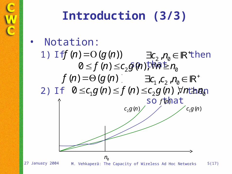
• Notation:1) If then so that

2) If then so that

))(()( ngnf 021 ),()()(0 nnngcnfngc

1 2 0, ,c c n

0n

)(2 ngc )(1 ngc)(nf

( ) ( ( ))f n g n2 0,c n

2 00 ( ) ( ),f n c g n n n

6(17)M. Vehkaperä: The Capacity of Wireless Ad Hoc Networks 27 January 2004

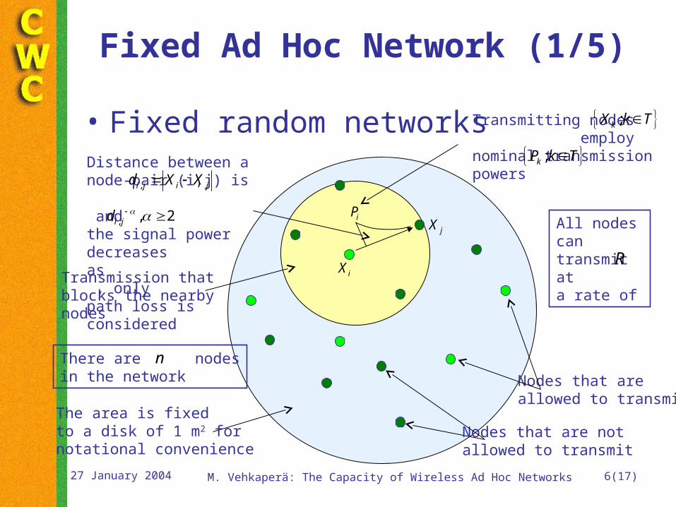
• Fixed random networks

Fixed Ad Hoc Network (1/5)

Nodes that areallowed to transmit

iX

jXiP

Nodes that are notallowed to transmit

The area is fixedto a disk of 1 m2 for notational convenience

Transmission that blocks the nearby nodes

Distance between a node-pair (i,j) is andthe signal power decreasesas , only path loss is considered

,i j i jd X X

, , 2i jd

Transmitting nodes employ nominal transmission powers

;kX k T

;kP k T

All nodes can transmit at a rate of R

There are nodesin the network

n

7(17)M. Vehkaperä: The Capacity of Wireless Ad Hoc Networks 27 January 2004

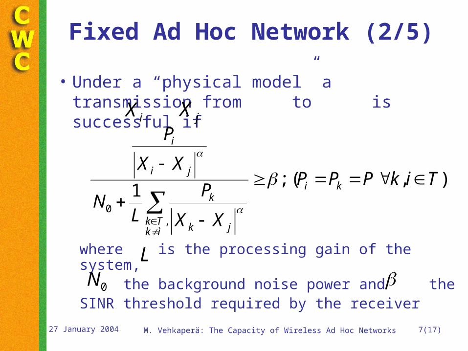
Fixed Ad Hoc Network (2/5)

• Under a “physical model” a transmission from to is successful if

where is the processing gain of the system, the background noise power and the SINR threshold required by the receiver

0,

; ( , )1

i

i j

i kk

k Tk jk ì

P

X XP P P k i T

PN

L X X

iX

L

0N

jX

8(17)M. Vehkaperä: The Capacity of Wireless Ad Hoc Networks 27 January 2004

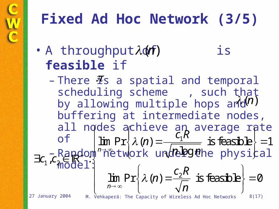
Fixed Ad Hoc Network (3/5)

• A throughput of is feasible if– There is a spatial and temporal

scheduling scheme , such that by allowing multiple hops and buffering at intermediate nodes, all nodes achieve an average rate of

– Random network under the physical model: 1

1 2

2

lim Pr ( ) is feasible 1log

, :

lim Pr ( ) is feasible 0

n

n

c Rn

n nc c

c Rn

n

( )n

( )n

9(17)M. Vehkaperä: The Capacity of Wireless Ad Hoc Networks 27 January 2004

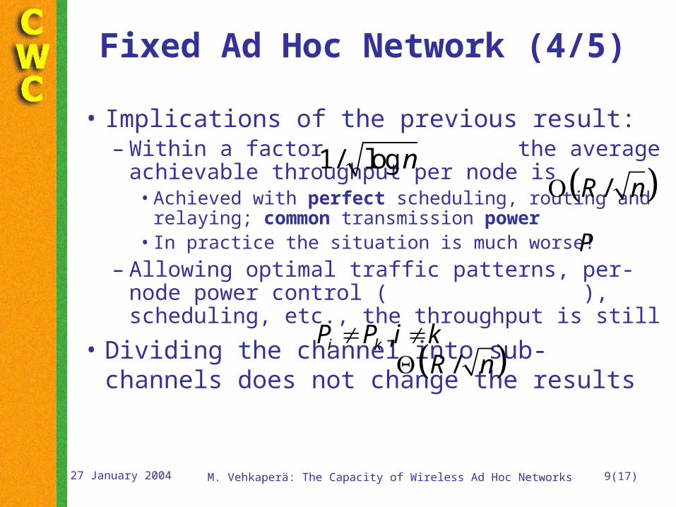
Fixed Ad Hoc Network (4/5)

• Implications of the previous result:– Within a factor the average

achievable throughput per node is• Achieved with perfect scheduling, routing

and relaying; common transmission power• In practice the situation is much worse!

– Allowing optimal traffic patterns, per-node power control ( ), scheduling, etc., the throughput is still

• Dividing the channel into sub-channels does not change the results

/R n1/ log n

,i kP P i k /R n

P

10(17)M. Vehkaperä: The Capacity of Wireless Ad Hoc Networks 27 January 2004

Fixed Ad Hoc Network (5/5)

• Conclusion from the results of [Gup00]:– What ever we do, the capacity of a fixed

wireless ad hoc network diminishes to zero as the “node-density” increases

• Why is the situation so pessimistic?– Throughput loss with common transmission

range is quadratic minimize – Small large number of intermediate

nodes per each “new” packet excessive relaying decreases the per-user throughput

– Lesson: Avoid dense ad hoc networks.

( )r n ( )r n( )r n

11(17)M. Vehkaperä: The Capacity of Wireless Ad Hoc Networks 27 January 2004

Mobile Ad Hoc Network (1/6)

• [Gro02]: With mobility, a constant per-user throughput when is possible– More nodes and movement, the better– True if the users are willing to wait (long..)– The delay is proportional to the speed of

change and the number of nodes in network• Works only with delay insensitive applications

– The users should also stay within a limited area or a large portion of packets is lost

– Not very realistic, but gives guidelines

n

12(17)M. Vehkaperä: The Capacity of Wireless Ad Hoc Networks 27 January 2004

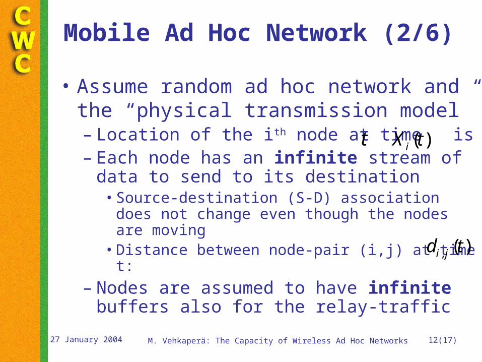
Mobile Ad Hoc Network (2/6)

• Assume random ad hoc network and the “physical transmission model”– Location of the ith node at time is – Each node has an infinite stream of

data to send to its destination• Source-destination (S-D) association does

not change even though the nodes are moving

• Distance between node-pair (i,j) at time t:

– Nodes are assumed to have infinite buffers also for the relay-traffic

( )iX tt

, ( )i jd t

13(17)M. Vehkaperä: The Capacity of Wireless Ad Hoc Networks 27 January 2004

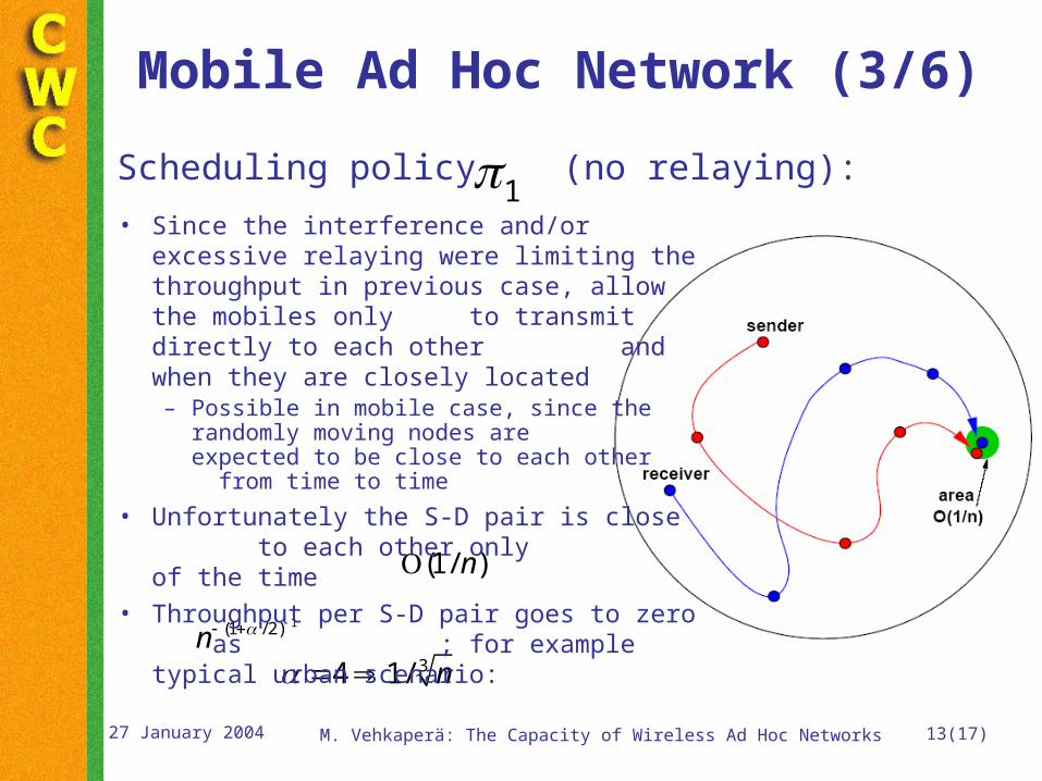
Scheduling policy (no relaying):

(1/ )n

Mobile Ad Hoc Network (3/6)

1(1 / 2)n

34 1/ n

1• Since the interference and/or

excessive relaying were limiting the throughput in previous case, allow the mobiles only to transmit directly to each other and when they are closely located– Possible in mobile case, since the

randomly moving nodes are expected to be close to each other from time to time

• Unfortunately the S-D pair is close to each other only of the time

• Throughput per S-D pair goes to zero as ; for example typical urban scenario:

14(17)M. Vehkaperä: The Capacity of Wireless Ad Hoc Networks 27 January 2004

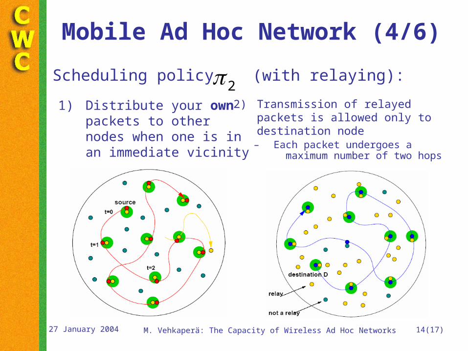
Mobile Ad Hoc Network (4/6)

1) Distribute your own packets to other nodes when one is in an immediate vicinity

2) Transmission of relayed packets is allowed only to destination node

– Each packet undergoes a maximum number of two hops

Scheduling policy (with relaying):2

15(17)M. Vehkaperä: The Capacity of Wireless Ad Hoc Networks 27 January 2004

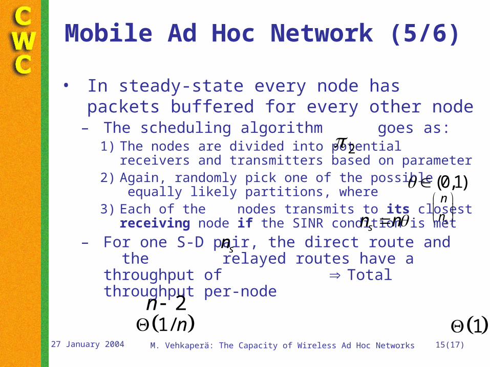
Mobile Ad Hoc Network (5/6)

• In steady-state every node has packets buffered for every other node

– The scheduling algorithm goes as:1) The nodes are divided into potential receivers

and transmitters based on parameter2) Again, randomly pick one of the possible

equally likely partitions, where3) Each of the nodes transmits to its closest

receiving node if the SINR condition is met

– For one S-D pair, the direct route and the relayed routes have a throughput of Total throughput per-node

(0,1)

s

n

n

2

sn nsn

1/ n2n

1

16(17)M. Vehkaperä: The Capacity of Wireless Ad Hoc Networks 27 January 2004

Mobile Ad Hoc Network (6/6)

• Conclusion from the results of [Gro02]:

– By assuming• Infinite length buffers and information streams• Users that are moving and stay in same area• Very loose delay constraints• Larger number of users (dense network)

– Throughput does not go to zero with !!– Scheduling policy can be implemented

also in a distributed manner

: lim Pr ( ) is feasible 1n

c n cR

2n

17(17)M. Vehkaperä: The Capacity of Wireless Ad Hoc Networks 27 January 2004

Conclusions

• Capacity of fixed and mobile wireless ad hoc networks was briefly examined

• Capacity of fixed network goes to zero as , regardless of the scheduling policy, routing, traffic patterns, etc..

• With loose delay constraints, the average asymptotic throughput per-node in mobile network is , that is, constant and non-zero

1/ n

1