Centre for Modeling and Simulation Savitribai Phule...

Centre for Modeling and SimulationSavitribai Phule Pune University

formerly University of Pune

+91.20.2560.1448 • +91.20.2569.0842cms.unipune.ac.in • [email protected]

Master of Technology (M.Tech.) Programmein Modeling and Simulation

Board of Studies: Modeling and SimulationFaculty of Technology, Savitribai Phule Pune University

Approved by Acadmic CouncilSavitribai Phule Pune University

August 8, 2016 (minor corrections, March 2018) • Version 3.141593

http://cms.unipune.ac.in/


http://www.unipune.ac.in/



mailto:[email protected]



About This Document

The Master of Technology (M.Tech.) Programme in Modeling and Simulation, designed by a core groupof people associated with the Centre for Modeling and Simulation, Savitribai Phule Pune University(formerly University of Pune), was approved by the University in 2007, and came into existence in theacademic year 2008-09. Based on the collective and individual experience gained since then, the presentdocument outlines a university-approved revision of this programme.

Citing This Document

Core Curriculum Team and Contributors, Master of Technology (M.Tech.) Programme in Modeling andSimulation 2016. Public Document CMS-PD-20160101 of the Centre for Modeling and Simulation,Savitribai Phule Pune University (formerly University of Pune), 2016.Available at http://cms.unipune.ac.in/reports.

Credits and Acknowledgements

Core Curriculum Team: Abhijat Vichare, Bhalchandra Pujari, Charulata Patil, Bhalchandra Gore,Sukratu Barve, Mihir Arjunwadkar.

Contributors: Abhijat Vichare, Vaishali Shah, Bhalchandra Pujari, Padma Pingale, Charulata Patil,Abhay Parvate, V. K. Jayaraman, Bhalchandra Gore, Sukratu Barve, Ashutosh Ashutosh, Mihir Arjun-wadkar.

Writing, Collation, Editing: Mihir Arjunwadkar.

Discussions and Advice: Professors Somnath Nandi, Lalitkumar Kshirsagar, Neeta Kankane, M. Y.Gokhale, Datta Dandage, Smita Bedekar.

Organizational Support: Professors Anjali Kshirsagar and Aditya Abhyankar.

Administrative Support: Jagruti Sondkar.

We Value Your Feedback

The utility of modeling and simulation as a methodology is extensive, and the community that uses it,academic or otherwise, is diverse. We would appreciate your feedback and suggestions on any aspect ofthis programme. Feedback can be sent to [email protected].

About the CentreThe Centre for Modeling and Simulation, Savitribai Phule Pune University(formerly University of Pune), was established in August 2003 with a vision topromote modeling and simulation methodologies and, in keeping with world-wide trends of modern times, to encourage, facilitate, and support highlyinterdisciplinary approaches to basic and applied research that transcend tra-ditional boundaries separating individual knowledge disciplines. For moreinformation, visit http://cms.unipune.ac.in/.

All models are false, some are useful.Quote attributed to George E.P. Box.




http://cms.unipune.ac.in/reports/pd-20160101/




http://cms.unipune.ac.in/reports

https://www.linkedin.com/pub/abhijat-vichare/2/822/828

http://cms.unipune.ac.in/~bspujari

http://cms.unipune.ac.in/~bwgore

http://cms.unipune.ac.in/~sukratu

http://cms.unipune.ac.in/~mihir


https://www.researchgate.net/profile/Vaishali_Shah10


https://jp.linkedin.com/in/abhay-parvate-5b808250

https://in.linkedin.com/in/jayaraman-valadi-a7916925



https://www.linkedin.com/profile/view?id=198572337




mailto:[email protected]





http://en.wikipedia.org/wiki/George_E._P._Box

CONTENTS 5

Contents

Administrative Summary of the Programme 8

1 The Revised M.Tech. Programme 91.1 What Has Not Changed . . . . . . . . . . . . . . . . . . . . . . . . . . . . . . . . 111.2 What Has Changed . . . . . . . . . . . . . . . . . . . . . . . . . . . . . . . . . . . 111.3 Core Courses . . . . . . . . . . . . . . . . . . . . . . . . . . . . . . . . . . . . . . 121.4 Choice-Based Courses (CBC) . . . . . . . . . . . . . . . . . . . . . . . . . . . . . 121.5 Internship . . . . . . . . . . . . . . . . . . . . . . . . . . . . . . . . . . . . . . . . 131.6 Professional Development Programme (PDP) . . . . . . . . . . . . . . . . . . . . 131.7 The M&S Course Stream . . . . . . . . . . . . . . . . . . . . . . . . . . . . . . . 131.8 Interpreting Syllabi . . . . . . . . . . . . . . . . . . . . . . . . . . . . . . . . . . . 141.9 Grading, Evaluation, Assessment . . . . . . . . . . . . . . . . . . . . . . . . . . . 141.10 The Student: Assumptions and Time Budgeting . . . . . . . . . . . . . . . . . . 151.11 Placement Activities . . . . . . . . . . . . . . . . . . . . . . . . . . . . . . . . . . 151.12 Course Prerequisites . . . . . . . . . . . . . . . . . . . . . . . . . . . . . . . . . . 15

2 Core Credits 172.1 Structure of the Core Curriculum . . . . . . . . . . . . . . . . . . . . . . . . . . . 192.2 C101 Real Analysis and Calculus . . . . . . . . . . . . . . . . . . . . . . . . . . . 212.3 C102 Vector Analysis . . . . . . . . . . . . . . . . . . . . . . . . . . . . . . . . . . 222.4 C103 Linear Algebra . . . . . . . . . . . . . . . . . . . . . . . . . . . . . . . . . . 232.5 C104 Ordinary Differential Equations . . . . . . . . . . . . . . . . . . . . . . . . 252.6 C105 Partial Differential Equations . . . . . . . . . . . . . . . . . . . . . . . . . . 272.7 C106 Probability Theory . . . . . . . . . . . . . . . . . . . . . . . . . . . . . . . . 292.8 C107 Computing with R . . . . . . . . . . . . . . . . . . . . . . . . . . . . . . . . 302.9 C108 Computing with MATLAB/Scilab . . . . . . . . . . . . . . . . . . . . . . . . 322.10 C109 Computing with C . . . . . . . . . . . . . . . . . . . . . . . . . . . . . . . . 332.11 C110 Algorithms . . . . . . . . . . . . . . . . . . . . . . . . . . . . . . . . . . . . 342.12 C111 M&S Hands-On 1 . . . . . . . . . . . . . . . . . . . . . . . . . . . . . . . . 362.13 C201 Complex Analysis . . . . . . . . . . . . . . . . . . . . . . . . . . . . . . . . 382.14 C202 Transforms . . . . . . . . . . . . . . . . . . . . . . . . . . . . . . . . . . . . 392.15 C203 Difference Equations . . . . . . . . . . . . . . . . . . . . . . . . . . . . . . . 412.16 C204 Numerical Computing 1 . . . . . . . . . . . . . . . . . . . . . . . . . . . . . 422.17 C205 Optimization 1 . . . . . . . . . . . . . . . . . . . . . . . . . . . . . . . . . . 442.18 C206 Statistical Inference . . . . . . . . . . . . . . . . . . . . . . . . . . . . . . . 462.19 C207 M&S Hands-On 2 . . . . . . . . . . . . . . . . . . . . . . . . . . . . . . . . 482.20 C301 Numerical Computing 2 . . . . . . . . . . . . . . . . . . . . . . . . . . . . . 492.21 C302 Optimization 2 . . . . . . . . . . . . . . . . . . . . . . . . . . . . . . . . . . 512.22 C303 Stochastic Simulation . . . . . . . . . . . . . . . . . . . . . . . . . . . . . . 522.23 C304 M&S Overview . . . . . . . . . . . . . . . . . . . . . . . . . . . . . . . . . . 542.24 C305 M&S Apprenticeship . . . . . . . . . . . . . . . . . . . . . . . . . . . . . . . 562.25 C401 Internship . . . . . . . . . . . . . . . . . . . . . . . . . . . . . . . . . . . . . 57

3 Choice-Based Credits: In-House Electives 593.1 Structure of the Choice-Based Curriculum . . . . . . . . . . . . . . . . . . . . . . 613.2 E001-1 Digital Signal and Image Processing 1 . . . . . . . . . . . . . . . . . . . . 633.3 E001-2 Digital Signal and Image Processing 2 . . . . . . . . . . . . . . . . . . . . 653.4 E002-1 Computational Fluid Dynamics 1 . . . . . . . . . . . . . . . . . . . . . . 673.5 E002-2 Computational Fluid Dynamics 2 . . . . . . . . . . . . . . . . . . . . . . 68

6 CONTENTS

3.6 E003-1 Machine Learning 1 . . . . . . . . . . . . . . . . . . . . . . . . . . . . . . 693.7 E003-2 Machine Learning 2 . . . . . . . . . . . . . . . . . . . . . . . . . . . . . . 713.8 E004-1 Operations Research 1 . . . . . . . . . . . . . . . . . . . . . . . . . . . . . 723.9 E004-2 Operations Research 2 . . . . . . . . . . . . . . . . . . . . . . . . . . . . . 733.10 E005 Concurrent Computing . . . . . . . . . . . . . . . . . . . . . . . . . . . . . 753.11 E006 High-Performance Computing . . . . . . . . . . . . . . . . . . . . . . . . . . 773.12 E007 Advanced Data Analysis . . . . . . . . . . . . . . . . . . . . . . . . . . . . . 793.13 E008 Computing with Java . . . . . . . . . . . . . . . . . . . . . . . . . . . . . . 803.14 E009 Theory of Computation . . . . . . . . . . . . . . . . . . . . . . . . . . . . . 813.15 E010 Functional Programming . . . . . . . . . . . . . . . . . . . . . . . . . . . . 833.16 E011 Computing with Python . . . . . . . . . . . . . . . . . . . . . . . . . . . . . 843.17 E012 Statistical Models and Methods . . . . . . . . . . . . . . . . . . . . . . . . . 85

4 Professional Development Programme (PDP) 874.1 Structure of the PDP Curriculum . . . . . . . . . . . . . . . . . . . . . . . . . . . 894.2 P001-1 Introduction to Linux 1 . . . . . . . . . . . . . . . . . . . . . . . . . . . . 914.3 P001-2 Introduction to Linux 2 . . . . . . . . . . . . . . . . . . . . . . . . . . . . 934.4 P002-1 Technical Communication 1 . . . . . . . . . . . . . . . . . . . . . . . . . . 944.5 P002-2 Technical Communication 2 . . . . . . . . . . . . . . . . . . . . . . . . . . 954.6 P003-1 Life Skills 1 . . . . . . . . . . . . . . . . . . . . . . . . . . . . . . . . . . . 964.7 P003-2 Life Skills 2 . . . . . . . . . . . . . . . . . . . . . . . . . . . . . . . . . . . 97

CONTENTS 7

8 CONTENTS

Administrative Summary: Master of Technology (M.Tech.) Pro-gramme in Modeling and Simulation

Title of the Programme Master of Technology (M.Tech.) Programme in Modeling and Simula-tion.

Degree Offered Master of Technology (M.Tech.) in Modeling and Simulation.

Designed by Centre for Modeling and Simulation, Savitribai Phule Pune Univer-sity (formerly University of Pune).

Board of Studies Modeling and SimulationFaculty Faculty of Technology, Savitribai Phule Pune University.

Mode of Operation Full-time, autonomous programme run by the Centre for Modelingand Simulation, Savitribai Phule Pune University in the academicflexibility/autonomy mode.

Minimum Duration 2 years.

Credits & Breakup Total credits: 100. Semester 1: 25 core credits. Semester 2: 18 coreand 7 choice-based credits. Semester 3: 15 core and 10 choice-basedcredits. Semester 4: 25 core credits.

Structure and Syllabus This document, Sec. 2 onwards.

Medium of Instruction English.

Number of Seats Regular Admissions. 30.Supernumerary Admissions. Sponsored Candidates: up to 10% of theregular seats. Foreign Students, Kashmiri Students, Etc.: as per theprevailing Savitribai Phule Pune University policies.

Fees Regular Admissions, Kashmiri Students, Foreign Students. As perthe prevailing Savitribai Phule Pune University policies for self-supporting departments.Sponsored Candidates. 2 × regular fees for the Maharashtra opencategory.

Eligibility {B.E./B.Tech. any branch} AND {Profficiency in Mathematics at12+2-level engineering (i.e., M1+M2+M3) programmes of SavitribaiPhule Pune University}

Admissions (First Year) Regular Admissions Including Kashmiri Students. Performance inan entrance test to ascertain adequate mathematics backgroundequivalent to 12+2-level science (S.Y.B.Sc.) and engineering(M1+M2+M3) programmes of Savitribai Phule Pune University,with a selection threshold/cutoff to be decided by the Centre forModeling and Simulation and declared in advance. These admis-sions will be subject to the prevailing Savitribai Phule Pune Univer-sity admission policy.Sponsored Candidates. First-come-first-served basis; separate en-trance test if number of candidates is greater than available seats.Foreign Students. Academic record, statement of purpose, and ac-ceptable English language skills. Telephonic interview and/or lettersof recommendation, if necessary, on a case basis.

Admissions (Second Year) As per the prevailing Savitribai Phule Pune University norms. Cur-rently, pass or better grade in at least 50% of the first-year credits.



















9

1 The Revised M.Tech. Programme

10 1 THE REVISED M.TECH. PROGRAMME

1.1 What Has Not Changed 11

1.1 What Has Not Changed

The Master of Technology (M.Tech.) Programme in Modeling and Simulation, publically availablein the form of public document CMS-PD-20070223 (http://cms.unipune.ac.in/reports/pd-20070223/), was designed by a core group of people associated with the Centre for Modelingand Simulation, Savitribai Phule Pune University (formerly University of Pune) after extensivebrain-storming and discussions, several preliminary revisions, and incorporating feedback fromexperts, both from academics as well as industry/corporate world. This programme was ap-proved by the University in 2007, and came into existence in the academic year 2008-09. Trueto the vision with which the Centre was founded in 2003, namely, to

promote modeling and simulation methodologies and, in keeping with worldwide trendsof modern times, to encourage, facilitate, and support highly interdisciplinary approachesto basic and applied research that transcend traditional boundaries separating individualknowledge disciplines,

the programme’s outlook and, consequently, its curriculum, have been multi-disciplinary tothe core right from the beginning – The original programme document cited above amplycorroborates this claim.

Therefore, what has not changed in this revision is

1. our philosophy and outlook on M&S;

2. our academic outlook including pedagogy, emphasis on concept over mathematical rigour,teacher’s freedom in choosing the mode/model of course delivery, etc.;

3. the goals of the programme;

4. the broad content of the programme (i.e., applied mathematics, applied statistics, com-puting, and M&S); and

5. preference for open-source software over proprietary/commercial software.

In this connection, we refer the reader to sections 1 and 2, and appendix I of the originalprogramme document cited above.

1.2 What Has Changed

The curriculum for the Master of Technology (M.Tech.) Programme in Modeling and Simulationhas been revised in the light of

1. experience gathered while running the programme since 2008;

2. feedback from students, alumni, teachers, employers, and experts;

3. better understanding of the student audience for this programme;

4. changes in the outside world; and

5. greater emphasis on depth while reducing the breadth of the original programme slightly.

Major changes incorporated in this revision of the programme are as follows:

1. Greater emphasis on the M&S component of the programme so as to convey the spirit ofM&S better, and revised structure and content for the M&S courses (Sec. 2). This pointis further elaborated upon in Sec. 1.7.

2. Additions, deletions, and content changes to core and elective courses (Sec. 2 and 3).

3. Greater flexibility offered to the student in terms of choice-based credits with a view tomake the programme more learner-centric (Sec. 1.4).

4. A focused professional development programme for the students (Sec. 1.6).

5. Revised operating guidelines, policies, and clarifications (the rest of this section).









1.3 Core Courses

Major changes to the core courses include

1. Technical communication and linux-related courses, which were part of the core curriculumin the original version, are now introduced as workshop-mode non-credit courses (Sec. 1.6).

2. The programming languages included in the core curriculum are C, MATLAB/Scilab, andR. C++ has been dropped. Java is now offered as an choice-based elective course.

3. Based on feedback from alumni and experts, the course on high-performance computingis now offered as a choice-based course.

4. A full-fledged course on numerical linear algebra has similarly been downsized and sub-sumed into a numerical computing course.

5. The M&S courses, which form the heart of the curriculum, now have a better-definedstructure and content.

6. Courses are now restructured to emphasize hands-on work and their “applied” aspect.

7. Courses on difference equations and discrete mathematics have been introduced in thecurriculum.

Detailed syllabi for the core courses can be found in Sec. 2.

1.4 Choice-Based Courses (CBC)

Aligning the Master of Technology (M.Tech.) Programme in Modeling and Simulation with theUGC’s recommendations for a choice-based credit system in spirit, the programme offers certainnumber of choice-based credits (Sec. 3). In contrast to an undergraduate student who is likely toconsider and explore a wide range of educational and career possibilities, a postgraduate studentis already far more specialized in her/his area of interest/expertise, and the choice (s)he wouldrequire is somewhat narrower compared to an undergraduate, and limited to technical areasof her/his interest or intended field of specialization. In the current curriculum, choice-basedcourses are offered in the second and third semesters once a student is adequately preparedfor them in the first semester. Academic and procedural guidelines for choice-based/electivecourses are as follows.

1. The in-house elective courses outlined in Sec. 3.

2. Any course proposed and approved by the Centre’s faculty/departmental committee af-ter thorough discussion and adequate revision, followed by approval from the Board ofStudies. Proposal should provide motivation/justification for the course, a well-designedsyllabus together with projected pedagogic and logistic requirements, and identify ade-quately qualified potential instructors (not necessarily from the Centre).

3. University-approved courses being offered at other University departments, centres, schools,affiliated entities outside the campus, and national institutes, provided the offering en-tity/instructor is willing to engage the interested students with adequate course work, aclear connection with M&S can be identified, and the Centre’s faculty deems such a courseas appropriate/suitable for the programme.

4. Ideally, it would be nice if the second elective taken by a student is a logical continuationof the first. However, this is not an absolute requirement, and a student may opt forelectives on two separate topics, provided pre-requisites/dependencies as laid out by thesyllabus and/or the instructor of the second course are satisfied.

1.5 Internship 13

5. A student needs to inform the Centre about her/his choice of elective courses for an up-coming semester at least a month in advance before the commencement of the semester.A student may be allowed to change their chosen elective/s within 3 weeks of the com-mencement of a semester, provided pre-requisites/dependencies of the second course aresatisfied. This applies both to the students in the Master of Technology (M.Tech.) Pro-gramme in Modeling and Simulation, as well as Savitribai Phule Pune University studentswishing to take credit courses at the Centre.

6. A student in the Master of Technology (M.Tech.) Programme in Modeling and Simulationmay take 17 credits worth of choice-based courses during semesters 2 and 3.

1.5 Internship

Continuing with the original vision of the programme, and based on the positive feedback fromadvisors/mentors from industry and academics alike, we have retained a full-semester full-time25-credit internship component in the curriculum. In our experience, this ensures substan-tial hands-on experience and domain-specific training, allows for out-of-town internships, thusmaximizing a student’s prospects for employment. Detailed information including operationalguidelines, pre-requisites, etc., for this component can be found in Sec. 2.25.

The internship component of the Master of Technology (M.Tech.) Programme in Modelingand Simulation may also be considered choice-based, because the choice of place, advisor, andtopic of internship lies entirely with the student, provided the internship is aligned with theoverall goals of the programme.

1.6 Professional Development Programme (PDP)

Recognizing certain shortcomings in the average student’s background and grooming, we havedesigned a professional development programme (PDP) for the students in the Centre’s academicprogrammes. This programme will be run every semester in a workshop mode with the help of in-house and/or outside experts. Parts of the this programme may be offered for a fee as certificatecourses open to the public. For students in the Master of Technology (M.Tech.) Programmein Modeling and Simulation, these workshops will be treated as additional 1-credit coursesrequiring mandatory attendance and participation, but without any assessment, evaluation, orgrading. Focus statements, rather than “syllabi”, can be found in Sec. 4.

The Professional Development Programme (PDP) consists of two course streams (namely,linux operating system and technical communication) that were part of the original curriculum,plus a life skills component. The life skills component of the PDP is motivated by the factthat many post-graduate students appear to lack independence, motivation, resourcefulness,and self-study skills; problem-solving skills; ability to think and organize knowledge; ability tomake connections across courses; time and work management skills; and sometimes even thebasic skills such as attention, listening, reading, and self-study that are taken for granted (see,e.g., Sec. I.1 of the original programme document http://cms.unipune.ernet.in/reports/

pd-20070223/). This often results into a mindless pursuit of degrees without enhancing realcapabilities, skills, or knowledge. This stream of the PDP is an attempt to make a student awareof possibilities and techniques that can help her or him be better-prepared for the world. Thelife skills component will be conducted with the help of qualified experts such as psychologists.

1.7 The M&S Course Stream

A criticism on the earlier curriculum for the programme was that it was dominated by mathe-matics courses. The current revision has achieved to strike a better balance between the various


http://cms.unipune.ernet.in/reports/pd-20070223/



groups of courses in the curriculum. Specifically, excluding choice-based and internship credits,the credit breakup for the four principal groups is as follows:

Course Group Courses Credits (%)

Mathematical C101–C107, C201, C203 19 (33%)Computing C108–C110, C202, C205, C301 10 (17%)Statistical/Stochastic C204, C206, C302, C303 12 (21%)M&S C111, C207, C304, C305 17 (29%)

Percentages reported with respect to core credits (58); this excludes internship (25) and choice-based credits (17).

We would like to point out the following in this regard.

1. The M&S course sequence C111 – C207 – C304 is based on the philosophical viewpointof first exposing the student to M&S ideas through hands-on work, and then presentingknowledge organization and systematization in the end.

2. The M&S course sequence C111 – C207 – C305 can be thought of as reducing the studentgroup size from entire class to individual, gradually driving a student towards indepen-dence, eventually culminating into the Internship C401.

1.8 Interpreting Syllabi

The syllabi in Sec. 2, 3, and 4 are to be considered indicative of the overall focus and scopeof the respective courses. Actual coverage of topics, their relative emphasis, and choice ofmodeling contexts may vary at the discretion of a competent instructor without compromisingupon the essential content and the goals for the course. Topics marked Optional may be coveredor not covered at the discretion of the instructor, the consideration here being the batch-to-batch variation in the students’ backgrounds, capabilities, and interests. The overall outlookon pedagogy (e.g., emphasizing concept and clarity over mathematical rigour; see Sec. I.2 ofthe original programme document (http://cms.unipune.ernet.in/reports/pd-20070223/)continues to underline the programme. Individual courses have been assigned two types ofcourse attribution: (a) Exactly one out of the set {Core, CBC, PDP}; and (b) one or more outof the set of {C (classroom), T (tutorial), L (laboratory), S (seminar), W (workshop)}. The(b)-attributions are suggestive of the pedagogic distribution of the course and of how the coursemay be conducted.

1.9 Grading, Evaluation, Assessment

We follow prevailing University policies and practices in this regard. Currently, continuousand final assessments have 50% weight each. It is also customary in the University to gradestudents using marks and then convert the resulting percentages to grades as per the University-prescribed norms. Beyond this, the teacher is the best judge of the mode/model of assessmentfor her/his course. On academic grounds, we refrain from making rigid and un-academic con-nections between nominal marks and duration of examination. Following the spirit of thechoice-based credit system, and in the best interest of the student, we also believe that final as-sessment/examination for a credit course should be at the end of the course, and not necessarilyat the end of the semester. Grades will be reported on the University-recommended 10-pointgrade scale1, or as per the prevailing rules and norms of the University.

1http://www.unipune.ac.in/university_files/pdf/CBCS-Handbook-28-7-15.pdf


http://www.unipune.ac.in/university_files/pdf/CBCS-Handbook-28-7-15.pdf

1.10 The Student: Assumptions and Time Budgeting 15

1.10 The Student: Assumptions and Time Budgeting

In formulating this intensive full-time programme, we have assumed that the student has

1. adequate level of motivation and interest in the programme, adequate time at hand, andthe ability to work hard; and

2. adequate background in mathematics, and capability of absorbing and assimilating theprogramme content.

Specifically, we have assumed that, on the average, the student will be able to put in 1–1.5 hoursof self-study for every hour of intensive academic engagement (i.e., classroom sessions). Giventhese assumptions, and reasonable assumptions about personal and commute time,

1. intensive academic engagement (i.e., classroom sessions), on the average, should not bemore than 5 clock hours on a typical working day;

2. any additional engagement, if necessary, should allow enough time for self-study, comple-tion of assignments, etc.; and

3. Centre’s library, computational laboratories, and internet/network resources should beavailable to the student after office hours as well, and should be adequate in capacity toaccommodate all admitted students simultaneously.

1.11 Placement Activities

Potential students often ask whether the Centre organizes campus placement activities. Ideally,campus placement activities should be run in an organized manner at the University level, wherenumbers and diversity are the key attractions for potential employers to engage with students.If this is not feasible, then we believe that campus placement is an area that is primarily of thestudents, by the students, for the students, and the Centre can at best be in a passive supportiverole. The Centre thus encourages and supports students in organizing such activities themselvesor in collaboration with students from other University departments, schools, or centres.

1.12 Course Prerequisites

The Common prerequisite (CP) for ALL courses (except courses under the Professional Develop-ment Programme, Sec. 1.6): Profficiency in Mathematics at 12+2-level science (i.e., S.Y.B.Sc.)and engineering (i.e., M1+M2+M3) programmes of SPPU. Course-specific prerequisites arespecified in Sec. 2.1, 3.1, and 4.1, as well as on individual course pages. Prerequisites needto be expanded recursively to get the full set of prerequisites for a course. Prerequisites fora course are interpreted as indicative of the minimum background necessary to assimilate thecourse content meaningfully.

17

2 Core Credits

18 2 CORE CREDITS

2.1 Structure of the Core Curriculum 19

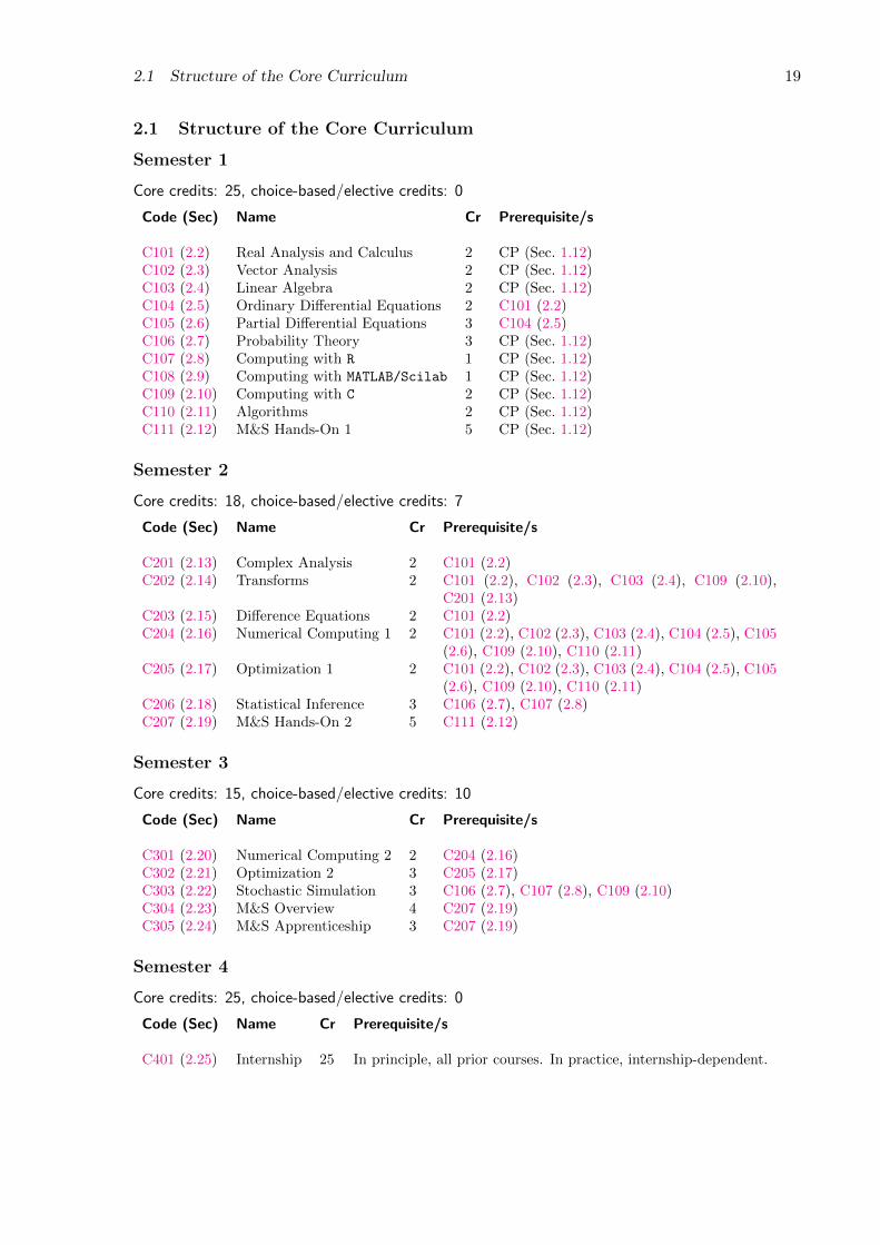
2.1 Structure of the Core Curriculum

Semester 1

Core credits: 25, choice-based/elective credits: 0

Code (Sec) Name Cr Prerequisite/s

C101 (2.2) Real Analysis and Calculus 2 CP (Sec. 1.12)C102 (2.3) Vector Analysis 2 CP (Sec. 1.12)C103 (2.4) Linear Algebra 2 CP (Sec. 1.12)C104 (2.5) Ordinary Differential Equations 2 C101 (2.2)C105 (2.6) Partial Differential Equations 3 C104 (2.5)C106 (2.7) Probability Theory 3 CP (Sec. 1.12)C107 (2.8) Computing with R 1 CP (Sec. 1.12)C108 (2.9) Computing with MATLAB/Scilab 1 CP (Sec. 1.12)C109 (2.10) Computing with C 2 CP (Sec. 1.12)C110 (2.11) Algorithms 2 CP (Sec. 1.12)C111 (2.12) M&S Hands-On 1 5 CP (Sec. 1.12)

Semester 2



C201 (2.13) Complex Analysis 2 C101 (2.2)C202 (2.14) Transforms 2 C101 (2.2), C102 (2.3), C103 (2.4), C109 (2.10),

C201 (2.13)C203 (2.15) Difference Equations 2 C101 (2.2)C204 (2.16) Numerical Computing 1 2 C101 (2.2), C102 (2.3), C103 (2.4), C104 (2.5), C105

(2.6), C109 (2.10), C110 (2.11)C205 (2.17) Optimization 1 2 C101 (2.2), C102 (2.3), C103 (2.4), C104 (2.5), C105

(2.6), C109 (2.10), C110 (2.11)C206 (2.18) Statistical Inference 3 C106 (2.7), C107 (2.8)C207 (2.19) M&S Hands-On 2 5 C111 (2.12)

Semester 3



C301 (2.20) Numerical Computing 2 2 C204 (2.16)C302 (2.21) Optimization 2 3 C205 (2.17)C303 (2.22) Stochastic Simulation 3 C106 (2.7), C107 (2.8), C109 (2.10)C304 (2.23) M&S Overview 4 C207 (2.19)C305 (2.24) M&S Apprenticeship 3 C207 (2.19)

Semester 4



C401 (2.25) Internship 25 In principle, all prior courses. In practice, internship-dependent.

20 2 CORE CREDITS

2.2 C101 Real Analysis and Calculus 21

2.2 C101 Real Analysis and Calculus

Credits. 2

Prerequisites. CP (Sec. 1.12)

Dependent Courses. Nearly all courses!

Attributions. Core; C, T

Rationale, Outlook, Purpose, Objectives, and Goals. Ability to apply standard calcu-lus techniques with good comfort levels regarding their basic understanding. The student shouldalso be able to handle real numbers and their analysis as much as outlined in the syllabus. Ifthe student so desires, he/she should be able to build upon this preparation independently todelve into elementary understanding (including proofs and heuristics) as and when needed inlater courses.

Syllabus.

1. Basics of set theory, relations and functions.

2. Introduction to metric spaces, open and closed sets, countable sets.

3. Real numbers, real sequences, infinite series, convergence and tests of convergence.

4. Real functions of single and several real variables, plotting graphs of such functions, limits,continuity and uniform continuity.

5. (For real functions of one real variable:) Derivative, Rolle’s and Lagrange mean valuetheorems, Taylor’s theorem, order notation and concept of infinitesimal, extreme valuesand indeterminate forms.

6. (For real functions of several real variables:) Differentiability, Young and Schwarz the-orems, partial derivatives, Taylor’s theorem and extreme values, homogeneous functionsand Euler’s theorem, implicit functions, Jacobians.

7. Revision of integration of functions of one variable, definition, standard results and meth-ods of integration, interpretation as area under graph, infinitesimals and Riemann sums.

8. Double integration with procedure and interpretation, Fubini’s theorem, change of vari-ables.

9. Triple integration with procedure.

Suggested Texts/References.

1. S. C. Malik and Savita Arora, Mathematical Analysis. New Age Publishers, 2009.

2. Erwin Kreyszig, Advanced Engineering Mathematics. Wiley India, 2014.

Notes on Pedagogy. Depending upon the capacity of the batch of students, previous orien-tation and training, the teacher can adjust the depth of delivery so as to best meet the objective.The content can also be tuned accordingly. The content could even be ordered and modifiedaccording to the presentation in the prescribed text book/s.

Contributor/s. Sukratu Barve (http://cms.unipune.ac.in/~sukratu)



22 2 CORE CREDITS

2.3 C102 Vector Analysis

Credits. 2




Rationale, Outlook, Purpose, Objectives, and Goals. This foundational course is in-tended to bring the student at an acceptable level of understanding of vector analysis so that(s)he is able to assimilate related material in advanced courses later on in the programme.

Syllabus.

1. Scalar and vector fields, surfaces and curves in space, examples using analytical geometry,parametric equations for curves and surfaces, intrinsic dimension of subsets of backgroundspace using analytical geometry.

2. Continuity and differentiability of vector and scalar fields. Partial derivatives of vectorsand scalar fields, the vector operator ∇.

3. Gradient of a scalar field, level surfaces, directional derivative and interpretation of gra-dient, tangent plane and normal to level surfaces.

4. Divergence and curl expressions. Important vector and scalar calculus identities.

5. Flux of a vector field through a surface portion with an example calculation.

6. Gauss Divergence theorem and outline of proof. Interpretation of divergence in terms offlux.

7. Vector line differential and integral with example calculations.

8. Deriving Green’s theorem in a plane. Definition of vector line integral (for 2D vectors ona plane) and relation to Green’s theorem.

9. Stokes’ theorem and outline of proof (e.g., using Green’s theorem). Interpretation of curlin terms of vector line integrals.

10. Conservative vector fields, line integrals and gradients: basic results with proofs, irrota-tional and solenoidal vector fields.



2. A. R. Vasishtha and Kiran Vasishtha, Vector Calculus. Krishna Prakashan Media, 2007.

3. Anil Kumar Sharma, A Textbook of Vector Calculus. Discovery Publishing House, 2006.

4. Shanti Narayan and P. K. Mitta, A Textbook of Vector Calculus. S. Chand, 1987.

Notes on Pedagogy.




2.4 C103 Linear Algebra 23

2.4 C103 Linear Algebra

Credits. 2




Rationale, Outlook, Purpose, Objectives, and Goals. This foundational course is in-tended to bring the student at an acceptable level of understanding of linear algebra so that(s)he is able to assimilate related material in advanced courses later on in the programme.

Syllabus.

1. Introduction to Matrices. Definition and examples, types of matrices, operations on and ofmatrices (row, column, sum, product, transpose, inverse, Hermitian adjoint) submatrices,determinants, rank, basic theorems on row and column operations on products, theo-rem on rank of product, elementary matrices, minors, Cofactors, and Cofactor adjointof a matrix, relation to inverse, standard properties of matrices,symmetry and similaritytransformations of matrices.

2. Systems of Linear Equations. Examples, solution methods (Gauss elimination), matrix rep-resentation and row echelon form of matrices, basic and free variables, consistency, numberof independent equations, Gauss-Jordan Elimination, Cramer’s rule and derivation, LUand LDU decomposition.

3. Vector Spaces. Outline of abstract algebra, groups, rings and fields. Definition of vectorspace over a field and examples of 3D vectors,functions,matrices and their appearance incontext of statistics and engineering. Basic results following immediately from axioms.Vector subspaces, linear independence, span, bases, uniqueness of coefficients, dependencetheorem, dimension and its uniqueness, direct sums, Transformation of bases.

4. Linear Operators. Definition and properties following immediately from definition. Nullspace and range. Bases and representation of linear operators as matrices, transformationof operator matrices according to basis transformations, examples.

5. Inner Product Spaces. Definition and basic properties, examples in 3d vectors and spacesof functions, Bessel inequality, Cauchy-Schwarz inequality, Norm from inner product andindependent definition of norm. Parallelogram and polarization identities. Angle betweenvectors and orthogonality (with examples from function spaces). Orthogonal complementof a subset, Orthonormal vectors, their linear independence, Gram-Schmidt Orthogonal-ization, projection operators and orthogonal projection operators, QR decomposition.

6. Eigenvalues, Eigenvectors and Diagonalization. Definition of eigenvectors and eigenvalues oflinear operators. Basic results. Calculation using matrix representations. Diagonalizationusing a particular similarity transformation, application in linear equations and linearODEs, normal matrices and diagonalizability, spectral theorem for normal matrices.

7. Quadratic forms. Definition, matrix of quadratic form and its symmetrization, definiteness,symmetry transformations and diagonal form, signature, Sylvester’s law of inertia, criteriafor definiteness, semidefiniteness and indefiniteness. Introduction to higher-degree forms.

24 2 CORE CREDITS


1. A.K. Lal, Notes on Linear Algebra. NPTEL, 2013. http://home.iitk.ac.in/~arlal/

book/nptel/pdf/book_linear.pdf

2. Kanti Bhushan Datta, Matrix and Linear Algebra. Prentice Hall India, 2008.

3. S. Kumaresan, Linear Algebra: A Geometric Approach. Prentice Hall India, 2000.

4. S.K. Mapa, Higher Algebra: Abstract and Linear. Levant Books, 2011.

5. Seymour Lipschutz and Marc Lipson, Linear Algebra (Schaum Series). McGraw-HillIndia, 2005.

6. Otto Bretscher, Linear Algebra with Applications. Pearson, 2008.

7. Paul Halmos and John L. Kelley, Finite Dimensional Vector Spaces. Literary Licensing,LLC, 2013.

8. Anil Kumar Sharma, Linear Algebra. Discovery Publishing House, 2007.

9. Georgi Shilov, Introduction to the Theory of Linear Spaces. Martino Fine Books, 2013.

Notes on Pedagogy.


http://home.iitk.ac.in/~arlal/book/nptel/pdf/book_linear.pdf

http://home.iitk.ac.in/~arlal/book/nptel/pdf/book_linear.pdf



2.5 C104 Ordinary Differential Equations 25

2.5 C104 Ordinary Differential Equations

Credits. 2

Prerequisites. C101 (2.2)

Dependent Courses. C105 (2.6), C204 (2.16), C301 (2.20), E002-1 (3.4), E002-2 (3.5)


Rationale, Outlook, Purpose, Objectives, and Goals. This and two sister courses C105(2.6) and C107 (2.8) aim at developing commonly-used modeling formalisms for describingchange.

Syllabus.

1. Definition of an ordinary differential equation, order and degree along with examples,Definition of solution. General particular and singular solutions, homogeneous functions.

2. First order ODEs having homogeneous functions. Shift of origin change of variables forconverting to homogeneous form. Exact first order ODEs. Standard examples of exactODEs. Integrating factors. Standard examples of integrating factors in various categoriesof first order ODEs. Linear first order ODEs and integrating factor, Bernoulli’s ODEFirst order ODEs with higher degree and methods of solution (solvable for x, y or dy/dx)Clairaut’s form of first order ODE.

3. Second order ODEs (homogeneous and non-homogeneous).

4. ODEs with constant coefficients, (optional examples of analysis of spring-mass-dashpotsystem) differential operator and its polynomial, complementary and particular integrals,general procedure of obtaining solution.

5. ODEs with variable coefficients, method of variation of parameters (only in case of secondorder ODEs)

6. Revision of sequences, series and convergence. Series of functions, Power series, ratio test,radius of convergence, series solutions of ODEs, method exemplified in particular cases(second order ODEs) Bessel, Hermite and Legendre ODEs and their series solutions. Briefoutline of special functions and their properties.

7. Side conditions of ODEs and their illustration in all the above techniques.

8. Conversion of higher order ODEs into first order ODEs with several dependent variables.Linear ODEs with several dependent variables, matrix formulation, interpretation of char-acteristic vectors and characteristic values, stability. Applications of this in perturbationof ODEs. Discussion of examples of 6 DOF analysis, control systems stability criteria,predator-prey and chemical reaction ODEs.

9. Numerical methods. Truncation, concept and implementation, forward backward andcentral difference schemes. Reference to difference equations. Concepts of consistencyand stability. Iterative algorithms for solution of difference equations eg. Euler, Heunand Runge Kutta methods. Implicit methods and matrix inversion techniques of solution.Convergence of solutions. Lax theorem (without proof) Computer exercises (3 examplesfor explicit and 3 for implicit schemes).

10. (OPTIONAL) Existence and uniqueness of solutions of first order ODEs, normed vactorspace techniques, uniform continuity, Lifshitz functions and outline of Picard’s theorem.Linear ordinary differential operators and resolvents. Examples of resolvents in common

26 2 CORE CREDITS

linear ODEs. Relation of side conditions to resolvents. Qualitative analysis of ODEs:Limit sets, fixed points, limit cycles, basins of attractors, Poincare Bendixson theorem(without proof) Lienard’s theorem (without proof).


1. S. Balachandra Rao and H. R. Anuradha, Differential Equations with Applications andPrograms. Universities Press, 1996.

2. E. Rukmangadachari, Differential Equations. Dorling Kindersley India, 2012.

3. A. Chakrabarti, Elements of Ordinary Differential Equations and Special Functions. NewAge International, 1990.

4. E. A. Coddington and N. Levinson, Theory of ordinary Differential Equations. Tata-McGraw Hill, 1972.

5. G. F. Simmons, Differential Equations with Applications and Historical Notes. Tata-McGraw Hill, 1991.

6. G. F. Simmons and S. G. Krantz, Differential Equations: Theory, Techniques and Practice.Tata-McGraw Hill, 2007.

Notes on Pedagogy.




2.6 C105 Partial Differential Equations 27

2.6 C105 Partial Differential Equations

Credits. 3


Dependent Courses. C204 (2.16), C301 (2.20), E002-1 (3.4), E002-2 (3.5)



Syllabus.

1. Definition of partial differential equation. Order, dependent and independent variables,themes of classification and standard categories, first and second order PDEs; Laplace,heat and wave equations as basic examples of linear second order PDEs. Examples ofhigher order and non linear PDEs.

2. Cauchy Problems for First Order Hyperbolic Equations. Method of characteristics, Mongecone.

3. Classification of Partial Differential Equations. Normal forms and characteristics for sec-ond order PDEs. Principal symbol and quasilinear PDEs, classification of quasilinearPDEs, types of side conditions and principal symbols. General types of side conditionsoccurring in applications of hyperbolic, parabolic and elliptic PDEs.

4. Initial and Boundary Value Problems. Lagrange-Green’s identity and uniqueness by en-ergy methods.

5. (Optional) Stability theory. Energy conservation and dispersion.

6. Laplace equation. Mean value property, weak and strong maximum principle, Green’sfunction, Poisson’s formula, Dirichlet’s principle, existence of solution using Perron’smethod (without proof).

7. Heat equation. Initial value problem, fundamental solution, weak and strong maximumprinciple and uniqueness results (outline of proofs and emphasis on interpretations)

8. Wave equation. Uniqueness, D’Alembert’s method, method of spherical means, Duhamel’sprinciple: outline of proofs with emphasis on interpretation.

9. Methods of separation of variables for heat, Laplace and wave equations. Various othermethods of solution of PDEs and brief descriptions.

10. Finite difference method as numerical methods for PDEs. Finite Difference Operators,Finite Difference methods, FDM for 1D heat and wave equations, implicit and explicitmethods of solution,method of lines,Jacobi, Gauss Seidel and Relaxation methods (for2D Laplace and Poisson equations) von Neumann stability for difference equations andapplications to 2D heat and wave equations. Stability and convergence of matrix differencemethods.


1. Erich Zauderer, Partial Differential Equations of Applied Mathematics. Wiley, 2006.

2. K. Sankara Rao, Introduction to Partial Differential Equations. PHI Learning, 2010.

28 2 CORE CREDITS

3. Phoolan Prasad and Renuka Ravindran, Partial Differential Equations. New Age Pub-lishers, 2012.

4. Lokenath Debnath, Nonlinear Partial Differential Equations for Scientists and Engineers.Birkhauser, 2011.

5. Lawrence C. Evans, Partial Differential Equations. American Mathematical Society, 2010.

Notes on Pedagogy.




2.7 C106 Probability Theory 29

2.7 C106 Probability Theory

Credits. 3


Dependent Courses. C206 (2.18), C302 (2.21), C303 (2.22), E003-1 (3.6), E003-2 (3.7),E007 (3.12), E012 (3.17)


Rationale, Outlook, Purpose, Objectives, and Goals. Probability is the mathematicallanguage for quantifying uncertainty or ignorance, and is the foundation of statistical inferenceand all probability-based modeling. Goals: Good understanding of probability theory as thebasis for understanding statistical inference; familiarity with basic theory and pertinent mathe-matical results; emphasis on illustrating formal concepts using simulation; and some perspectiveon modeling using probability by way of real-life contexts and examples.

Syllabus.

1. Probability. Sample spaces and events. Probability on finite sample spaces. Independentevents. Conditional probability. Bayes’ theorem.

2. Random Variables. Distribution functions and probability functions. Important discreteand continuous random variables. Bivariate and multivariate distributions. Indepen-dent random variables. Conditional distributions. Important multivariate distributions.Transformations on one or more random variables.

3. Expectation. Properties. Variance and covariance. Expectation and variance for importantrandom variables. Conditional expectation. Moment generating functions.

4. Inequalities for Probabilities and Expectations. Markov, Chebychev, Hoeffding, Mill, etc.Inequalities for expectation: Cauchy-Schwartz, Jensen, etc.

5. Convergence and Limit Theorems. Notion of convergence for random variables. Types ofconvergence. Law of large numbers, central limit theorem, the delta method.

6. Stochastic Processes (Optional). Basic introduction to simple branching processes, randomwalks, Markov chains, etc.


1. Christopher R. Genovese, Working With Random Systems: Mechanics, Meaning, andModeling. Unpublished, 2000. http://www.stat.cmu.edu/~genovese/books/WWRS.ps

2. Charles M. Grinstead and J. Laurie Snell, Introduction to Probability. American Mathe-matical Society, 1997. https://math.dartmouth.edu/~prob/prob/prob.pdf

3. Morris deGroot and Mark Schervish, Probability and Statistics. Addison-Wesley, 2002.

4. Larry Wasserman, All of Statistics. Springer-Verlag, 2004 (Part 1 of the book).

5. David Stirzacker, Elementary Probability. Cambridge University Press, 1994.

Notes on Pedagogy. This course can go hand-in-hand with the Computing with R courseC107 (2.8). For example, R can be used liberally to illustrate (by the instructor) and explore(by the student) probability-related concepts and important results such as the central limittheorem.

Contributor/s. Mihir Arjunwadkar (http://cms.unipune.ac.in/~mihir)

http://www.stat.cmu.edu/~genovese/books/WWRS.ps

https://math.dartmouth.edu/~prob/prob/prob.pdf



30 2 CORE CREDITS

2.8 C107 Computing with R

Credits. 1


Dependent Courses. C206 (2.18), C303 (2.22), E003-1 (3.6), E003-2 (3.7), E007 (3.12),E012 (3.17)

Attributions. Core; L

Rationale, Outlook, Purpose, Objectives, and Goals. The R (http://cran.r-project.org/) statistical computing environment, built around the S programming language, is rich incomputational statistics primitives. It is open-source and supported by an ever-growing commu-nity of users and contributors. It allows a variety of programming styles from quick-and-dirtyexplorations to elaborate imperative, procedural, object-oriented, and functional coding. It isideally suited for statistical modeling and data analysis, graphics and visualization, as well asa platform for teaching/learning probability and statistics through hands-on exploration. Assuch, R is a must for any broad-based M&S curriculum with a statistical modeling/data analysiscomponent. Goals: proficiency in computational problem-solving using R; specifically, decentalgorithmic, coding, and scripting skills.

Syllabus.

1. Overview of R and S. History of R. Why use R? When not to use R? GUIs for R. Invok-ing and exiting the R interpreter environment. Getting help and finding information.demo(). The six atomic types. Assignment operators. Standard arithmetic and logicaloperators. Comments. Conditionals and loops. Parenthesis and braces. Expressions.Every expression has a value. Common composite data types: vector, list, matrix, anddata.frame. The elementwise operations rule for vector and related container types.functions. Writing and executing R scripts: source() and Rscript.

2. Case studies illustrating R capabilities, in-built functions, and common packages. Overview ofR graphics. Probability distributions and random number generators. Creating numericaland graphical data summaries, and exploratory data analysis. Complex numbers, numer-ical methods, etc. Character strings. Set operations. Interface to the operating systemshell. Data input and output.

3. Installing R and R packages locally into a linux user account. Installing R from source:configure – make – make install sequence. Installing packages: install.packages()

and the R CMD INSTALL mechanism.

4. Migrating from C to R. Automatic type identification in an assignment vs. explicit decla-ration of data type. ; and \n as expression terminators. Explicit loops vs. vectorization.

5. Getting performance from R codes. Coding style guidelines. Explicit loops vs. vectoriza-tion. The compiler package. Debugging and profiling tools. Interfacing with C, C++,

fortran.

6. Hands-on explorations using R. Any reasonable set of hands-on problems designed to en-hance computational problem-solving and algorithmic abilities. Such problems may berelated to M&S in general, or specifically to topics from other courses (e.g., probabilitytheory, statistical inference) in the programme or the instructor’s field of expertise.

http://cran.r-project.org/



2.8 C107 Computing with R 31


1. W. N. Venables, D. M. Smith, and the R Development Core Team, An Introduction toR. The R Project, latest available edition. http://cran.r-project.org/doc/manuals/

R-intro.html

2. John Verzani, Using R for Introductory Statistics. Chapman & Hall/CRC, 2005.

3. Daniel Navarro, Learning Statistics with R: A Tutorial for Psychology Students and OtherBeginners. Self-published, 2013. http://learningstatisticswithr.com/

4. Paul Murrell, R Graphics. Chapman & Hall/CRC, 2011.

5. Patrick Burns, The R Inferno. http://www.lulu.com/, 2012. Available at http://www.

burns-stat.com/documents/books/the-r-inferno/.

6. W. N. Venebles and B. D. Ripley, Modern Applied Statistics with S-Plus. Springer, 2002.

7. R. G. Dromey, How to Solve It By Computer. Prentice-Hall, 1982.

Notes on Pedagogy. This syllabus is based on an outline for a longer course that was re-fined over several course deliveries by the contributor (see below). Depending on the backgroundand capabilities of the students, this outline may need to be somewhat diluted or intensified –without compromising upon the essentials and goals for the course. Apart from familiarizing astudent with R, a major emphasis of this course is on tinkering and exploration, on computa-tional problem-solving, and on translating a problem into a computational framework leadingto either a solution or a better understanding of the problem, and on how R can be used as aM&S tool, and for exploring/visualizing probability and statistics concepts. Assignments oftenconsist of problems that are exploratory in nature (e.g., illustrating formal results that may bedifficult to grasp, such as the central limit theorem; see C106 (2.7)), or require a student tounderstand an algorithm from its plain-English or pseudocode description (e.g., generating thenext permutation given a permutation of n objects). Examinations may consist of problemsnot necessarily discussed in the class: Here, adequate information about the method of solutionor algorithm is provided.


http://cran.r-project.org/doc/manuals/R-intro.html

http://cran.r-project.org/doc/manuals/R-intro.html

http://learningstatisticswithr.com/

http://www.lulu.com/

http://www.burns-stat.com/documents/books/the-r-inferno/

http://www.burns-stat.com/documents/books/the-r-inferno/



32 2 CORE CREDITS

2.9 C108 Computing with MATLAB/Scilab

Credits. 1


Dependent Courses. C204 (2.16), C301 (2.20), E002-1 (3.4), E002-2 (3.5)


Rationale, Outlook, Purpose, Objectives, and Goals. MATLAB and its open-source par-allel Scilab are popular, powerful, and flexible platforms for numerical and symbolic computa-tion, visualization and graphics, etc., and are rich in computational primitives for diverse fieldsfrom digital signal processing to statistics. This course aims at developing an intermediate skilllevel in writing scripts, performing calculations, using the command line, importing data fromfiles, plotting data, and integrating with other programming languages such as C.

Syllabus.

1. Introduction. Environment. Workspaces. General syntax.

2. Numerics. Creating matrices. Matrix operations. Sub-matrices. Statistical operations.Polynomials, differential equations.

3. Plots. Plotting graphs for 2D, 3D functions. Various types of plots.

4. Programming. Functions, Scilab/MATLAB programming language, Script files and functionfiles.

5. I/O. Reading, writing data in various formats.

6. Interfacing with programming languages such as C.


1. Amos Gilat, MATLAB: An Introduction with Applications. Wiley, 2008.

2. Mathews and Fink, Numerical Methods Using MATLAB. Pearson, 2004.

3. J. C. Polking and D. Arnold, Ordinary Differential Equations using MATLAB. Pearson,2003.

4. An extensive comparison of MATLAB and Scilab: http://www.professores.uff.br/controledeprocessos-eq/images/

stories/Comparative-Study-of-Matlab-and-Scilab.pdf

Notes on Pedagogy. Case studies and problems used for introducing MATLAB/Scilab shouldideally be derived from other courses (e.g., differential equations C106 (2.7), C107 (2.8)) runningconcurrently.

Contributor/s. Bhalchandra Pujari (http://cms.unipune.ac.in/~bspujari)

http://www.professores.uff.br/controledeprocessos-eq/images/stories/Comparative-Study-of-Matlab-and-Scilab.pdf





2.10 C109 Computing with C 33

2.10 C109 Computing with C

Credits. 2


Dependent Courses. C202 (2.14), E005 (3.10), E006 (3.11)


Rationale, Outlook, Purpose, Objectives, and Goals. Upon successful completion ofthis course, the student is expected to be able to

1. Understand basics of procedural/functional programming, syntax, semantics of C.

2. Design an algorithm to solve problems of various kinds in modeling and simulation andimplement using C programming language.

3. Debug the code to spot logical errors, exceptions etc.

4. Write reasonably complex C code for solving various problems in modeling and simulation.

Syllabus.

• ANSI C. Syntax, data types, concept of void, variables, operators, expressions and state-ments, character input and output, console input and output, inclusion of standard headerfiles, pre-processor directives.

• Control flows. If-else, for, while, do-while, switch-case, break and continue, code blocksand nesting of blocks.

• Functions. Basics of functions, return statement, recursion, function blocks, static vari-ables

• Memory management. Dynamic versus static memory allocation, freeing memory, arrays,memory layout of multidimensional arrays.

• Pointers. Concept of pointers, pointer arithmetic, pointers versus arrays, array of pointers.

• Program compilation and debugging techniques. Introduction to tools like gdb togetherwith ddd, GNU make and profiler gprof. Code organization across files. Version/revisioncontrol using svn or git.

• Structures and Unions. Structures and unions, bit fields, typedef, self referential structures,their use in link-list, queue, stack etc.

• Input and output in C. Files, file operations.


• Kernighan and Ritchie, The C Programming Language. PHI, 1990.

• R. L. Kruse, B. P. Leung, C. L. Tondo, Data Structures And Program Design In C. PearsonEducation, 2007.

Notes on Pedagogy. Although finite-precision arithmetic is covered at length in the courseC201 (2.13), the student may be exposed here to the bare-basics of finite-precision representa-tions and arithmetic if time permits, and at the discretion of the instructor.

Contributor/s. Bhalchandra Gore (http://cms.unipune.ac.in/~bwgore)



34 2 CORE CREDITS

2.11 C110 Algorithms

Credits. 2


Dependent Courses. C204 (2.16), C205 (2.17), C301 (2.20), E005 (3.10), E006 (3.11), E008(3.13)

Attributions. Core; C, L

Rationale, Outlook, Purpose, Objectives, and Goals. This is intended to be an intro-duction to algorithms for a non-computer-science graduate student. In principle, any program-ming language (C, Python, Haskel, LISP, etc.) can be used for illustrating algorithms, at thediscretion of the instructor. However, C is highly recommended so as to give student a closerfeel of computer system organization. Please see the sister course C109 (2.10). This course isintended for

• familiarizing the student with the computer system organization and its use for problemsolving;

• making student understand the need for formal algorithm development; and

• introducing basic types of algorithms, design techniques, data structures used for problemsolving.

Syllabus.

1. Introduction to Algorithms. What is an algorithm, why do we need it? Introduction tofundamental algorithms like counting, sorting; algorithms for problem solving using digitalcomputers, flow chart and pseudocode techniques. [5-6 hrs.]

2. Algorithms. Fundamental algorithms and techniques, data structures required (queue,FIFO, FILO, LIFO, LILO terminologies, stacks, link-lists, trees and graphs), logic, settheory, functions, basics of number theory and combinatorics (sequences-series, Sigma andPI notations for termwise summation, multiplication, probability, permutations, combi-nations), mathematical reasoning–including induction. [10-12 hrs.]

3. Recursion. Need, advantages, disadvantages. Recurrence analysis. Introduction to re-currence equations and their solution techniques (substitution method, tree recursionmethod, master method). Proof of the master method for solving recurrences. Demon-stration of the applicability of master theorem to a few algorithms and their analysis usingrecurrence equations. Example algorithms: binary search, powering a number, Strassen’Smatrix multiplication, etc. [10-12 hrs.]

4. Types of Algorithms and Their Analysis. Theta and big-theta notation, θ and Θ notations;comparison of algorithms, notions of space and time efficiency; as an illustrative example,comparison of quick-sort algorithm with other sorting algorithms can be demonstrated.[5 hrs.]


• V. Rajaraman, T. Radhakrishnan, An Introduction to Digital Computer Design. PHI,2007.

• T. H. Cormen, C. E. Leiserson, R. L. Rivest, C. Stein, Introduction to Algorithms. PHILearning, 2009.

2.11 C110 Algorithms 35

• D. E. Knuth, The Art of Computer Programming, Vol. 1. Addison Wesley, 2011.

• A. V. Aho, J. E. Hopcroft, J. D. Ullman, Design and Analysis of Algorithms. PearsonEducation, 2011.

• E. Horowitz, S. Sahni, Fundamentals of Computer Algorithms. Universities Press, 2008.

Notes on Pedagogy.




36 2 CORE CREDITS

2.12 C111 M&S Hands-On 1

Credits. 5


Dependent Courses. C207 (2.19), C304 (2.23), C305 (2.24)

Attributions. Core; C, L, S

Rationale, Outlook, Purpose, Objectives, and Goals. It is a challenge to communicatethe depth of the sense in which modeling and simulation are to be understood. This coursestems from the belief that a hands on experience can build the intuition more strongly thanany other pedagogic technique. It proposes a reasonable cheap laboratory where students buildmodels of some problems, and try to answer questions using them. The models are necessarilyphysical. The degree of finesse that can be achieved is as much a function of creativity as it isof the cost. The kind of equipment available could start as simply as card boards, pins, glue,paper, colours for painting, wires, bread boards, small motors, or even waste material (e.g.broken toys, devices) etc.

This course is conceived as a first course, and hence has no “syllabus” as such. Instead it isa collection of some “simple”/“simplified” problems that should illustrate the nature of M&S.The key to the success is in grasp on M&S that a student achieves, and should answer basicquestions like:

1. What aspect/s of the reality does the model capture? What aspect/s does it not capture?

2. What questions can the model answer and what questions can it not answer? Why?

3. Is the model capable of simulation?

4. What questions need a simulation using the model to be answered? Are they differentfrom questions that the model can answer without simulation? If so, in what way?

5. . . .

6. Get introduced to M&S through actual experience.

7. What tools (mathematical, statistical, programmatic) are required to address problemsin a particular stream?

Syllabus. This is an open-ended course, and the instructor is the best judge of topics andcase studies to use to convey the spirit of M&S. At the discretion of the instructor, the selectioncase studies may include:

1. Study of internal combustion engines

2. Study of a plant cell or animal cell

3. Study of planetary motion of our solar system

4. Study of Newton’s Laws of motion (various: e.g. central force, projectiles etc.)

5. Study of equilibrium in chemical reactions

6. Study of mechanical adding machines

Suggested Texts/References. No specific texts or references. Instructor can choose anyappropriate selection of texts and references.

2.12 C111 M&S Hands-On 1 37

Notes on Pedagogy. The main thrust of this course should be to make students comfortablein applying their current knowledge of the modeling techniques to solve a variety of problems.The course may be run by assigning mini-projects to groups of students to generate physical,mathematical, programmatic models and demonstrate their usefulness/inadequacies. The de-liverable could be a physical model, a computer program (which is expected to follow basicsoftware development norms) or a proposal based on their study, etc. The exact nature of thedeliverable by students and the evaluation methodology is left to the instructor. Hence, thereare no prescribed reference books/articles. This course is also a placeholder for the top-downapproach to M&S. The students, through case studies, are supposed to understand the needfor more detailed study of mathematical, statistical and programmatic tools to understandintricacies of M&S.

Contributor/s. Abhijat Vichare (https://www.linkedin.com/pub/abhijat-vichare/2/822/828),Bhalchandra Gore (http://cms.unipune.ac.in/~bwgore), Abhay Parvate (https://jp.linkedin.

com/in/abhay-parvate-5b808250)








38 2 CORE CREDITS

2.13 C201 Complex Analysis

Credits. 2


Dependent Courses. C202 (2.14), E001-1 (3.2), E001-2 (3.3)


Rationale, Outlook, Purpose, Objectives, and Goals. Complex analysis is a powerfuland widely used area of mathematics with applicability in diverse areas of science and engi-neering. This foundational course is intended to bring the student at an acceptable level ofunderstanding of complex analysis so that (s)he is able to assimilate related material in ad-vanced courses later on in the programme.

Syllabus.

1. Complex Analytic Functions. Complex Numbers. Polar form of complex numbers, triangleinequality. Curves and regions in the complex plane. Complex function, limit, continuity,derivative. Analytic function. Cauchy-Riemann equations. Laplace’s equation. Rationalfunctions, roots, exponential function, trigonometric and hyperbolic functions, logarithm,general power.

2. Complex Integrals. Line integral in the complex plane. Basic properties of the complex lineintegral. Cauchy’s integral theorem. Evaluation of line integrals by indefinite integration.Cauchy’s integral formula. Derivatives of an analytic function.

3. Laurent Series. Review of power series and Taylor Series. Convergence. Uniform conver-gence. Laurent series, analyticity at infinity, zeros and singularities.

4. Complex Integration by Method of Residues. Analytic functions and singularities. Residues,poles, and essential singularities. The residue theorem. Contours. Contour integrationand Cauchy residue theorem as techniques for real integration. Principal values of inte-grals.


1. Tristan Needham, Visual Complex Analysis. Oxford University Press, 1999.


3. M. J. Ablowitz and A. S. Fokas, Complex Variables: Introduction and Applications. Cam-bridge University Press, second edition, 2003.

4. Arfken and Weber, Mathematical Methods for Physicists. Elsevier, 2005.

Notes on Pedagogy. On pedagogical note, it is important to remember that students will berequired to learn the evaluation of inverse integral transforms later in their course work. It wouldbe useful if the instructor motivates the students using this as application. The student shouldbe adequately familiarized with methods particularly useful in evaluating inverse transforms.




2.14 C202 Transforms 39

2.14 C202 Transforms

Credits. 3

Prerequisites. C101 (2.2), C102 (2.3), C103 (2.4), C109 (2.10), C201 (2.13)

Dependent Courses. E001-1 (3.2), E001-2 (3.3)

Attributions. Core; C, T, L

Rationale, Outlook, Purpose, Objectives, and Goals. Integral and discrete transformsare often useful in transforming a complex problem into a simpler one. Moreover, insights aboutthe system can be obtained through transforms. Needless to say that integral and discretetransforms are vital tools in the modeling and simulation premises. The goal of this course isto introduce students to a few commonly used transforms with substantial emphasis on Fouriertransform. A significant computing aspect is also expected. Students should be able to writecodes for some of the transforms. Students are also expected to learn to analyze the results oftransformed signals through computational platforms such as matlab/scilab/R.

Syllabus.

1. Introduction and background. Brief introduction to vector spaces, function spaces andbasis sets. Special functions. Function parity. Concepts in complex analysis. Kernel ofan integral transform.

2. Fourier series. Periodic functions. Fourier series in trigonometric as well as complexexponent representation. Functions with arbitrary period. Solving differential equationswith Fourier series.

3. Fourier transform. Fourier integrals. Fourier sine/cosine transforms. Fourier transform.Inverse Fourier transform. Properties of Fourier transform. Convolution. Applications.Solving differential equations using Fourier transform, Power spectrum and its interpre-tation.

4. Discrete Fourier transform and fast Fourier transform. Discretization. Sampling. Nyquistsampling. Discrete Fourier transform. Properties. Matrix representation of DiscreteFourier transform. Fast Fourier transform. Comparison.

5. Laplace transform. Laplace transform. Properties. Inverse transform using partial frac-tions, convolution and complex integration. Applications. Solution of differential equa-tions.

6. Wavelet transform. Limitations of Fourier transform. Introduction to wavelets and familyof wavelets. Translations and scaling. Continuous and Discrete wavelet transform. Haarscaling and wavelet functions. Functions spaces. Decomposition using Haar bases. Gen-eral wavelet system. Daubechies wavelets. Multiresolution analysis. Analysis of outputof wavelet transforms.

7. Z-transform. Definition of Z-transform. Properties. Inverse Z-translations using complexintegral methods. Difference equations.


1. L. C. Andrews and B. K. Shivamoggi, Integral Transforms for Engineers. Prentice-Hallof India, 2003.


40 2 CORE CREDITS

3. R. N. Bracewell, The Fourier transform and its applications. Tata McGraw-Hill, 2003.

4. L. Devnath and D. Bhatta, Integral transforms and their applications. Chapman andHall/CRC, 2010.

5. K. P. Soman and K. I. Ramchandran, Insights into wavelets - From theory to practice.Prentice-Hall India, 2005.

6. Online coursework such as Brad Osgood (Stanford), Alan Oppenheim (MIT), etc.

Notes on Pedagogy. An instructor may choose to alter the order to introduce the transforms.However it is logical to start with Fourier series for periodic function, followed by Fouriertransform for non-periodic function. The limitation of Fourier transform to resolve the functionin both frequency and time domains leads to use of Wavelet and on the other hand Laplacetransform can be viewed as ‘generalized’ Fourier transform, which takes into account the realpart of frequency. Similarly Z-transform can be seen as generalized discrete Fourier transform.

A significant emphasize is expected to be on students developing their own codes for varioustransforms.




2.15 C203 Difference Equations 41

2.15 C203 Difference Equations

Credits. 2


Dependent Courses. E002-1 (3.4), E002-2 (3.5)



Syllabus.

1. Definitions of difference equations (ordinary and partial) dependent and independent vari-ables, order and degree, types (linear, quasilinear) elliptic, hyperbolic and parabolic dif-ference equations. Types of side conditions for each.

2. Translation operator and algebraic methods to solve degree one homogeneous and inho-mogeneous difference equations. Similarity with ODE methods. Methods using the Ztransform.

3. Numerical methods of solution of ordinary difference equations. Examples of usage of datastructures and creation of algorithms in this context. Difference equations that result fromdiscretization of differential equations (two examples like Euler stepping and Runge Kuttamethod).

4. Translation operators for partial difference equations and algebraic methods for solvingbasic forms of partial difference equations analytically.

5. Numerical methods for partial difference equations, classification as sweeping and step-ping methods. Examples of usage of data structures and creation of algorithms in thiscontext. Difference equations that result from discretization of partial difference equations(examples of finite difference method only).

6. Application of difference equations in population dynamics and finance.

7. Introduction to theoretical concepts of stability, oscillation and asymptotic behaviour ofdifference equations and their solutions.


1. Saber N. Elaydi, Introduction to Difference Equations. Springer, 1999.

2. Ronald E. Mickens, Difference Equations. CRC Press, 1991.

3. Walter C. Kelley and Allan C. Peterson, Difference Equations: An Introduction withApplications. Academic Press, 2001.

4. Mathematical Modelling Through Difference Equations, Chapter 5, in: J. N. Kapur, Math-ematical Modelling. New Age International Publishers, 2008.

5. Sui Cun Cheng, Partial Difference Equations. Taylor and Francis, 2003.

Notes on Pedagogy.




42 2 CORE CREDITS

2.16 C204 Numerical Computing 1

Credits. 2

Prerequisites. C101 (2.2), C102 (2.3), C103 (2.4), C104 (2.5), C105 (2.6), C109 (2.10), C110(2.11)

Dependent Courses. C301 (2.20)


Rationale, Outlook, Purpose, Objectives, and Goals. Many modeling formalisms andsituations lead to formulations that involve the use of numerical computing, which we defineloosely as numerical analysis/mathematics plus a strong hands-on computing component. Thiscourse and its sister course C301 (2.20) are intended to cover topics of practical importancethat are not covered elsewhere in the curriculum.

Syllabus.

1. Finite-Precision Arithmetic. Computer representations of integers: Properties; overflowand roll-over; endianness. Computer representations of “real” numbers: Fixed-point andfloating-point; properties of floating-point numbers and representations (e.g., number anddistribution of representable floating-point numbers, overflow and underflow, machineepsilon, minimum and maximum representable number; etc.).

2. The Rounding Error. How elementary arithmetic operations are performed on floating-point numbers. How precision is lost in arithmetic operations such as subtraction. Exam-ples of loss of precision such as in computing roots of a quadratic equation, etc. Analysisof the rounding error for simple computations. Useful strategies for avoiding accumulationof rounding error; e.g., minimize arithmetic operations (e.g., Horner’s and other methodsfor polynomial evaluation), re-arrange computation to avoid subtraction of nearly equalfloating-point numbers (e.g., in computing roots of a quadratic equation when b2 ≈ 4ac),etc.

3. A User’s Perspective on the IEEE 754 Specification. IEEE 754 representations of floating-point types and their characteristics. IEEE 754 specifications for arithmetic operations.Special values: NaN, Inf, signed zero, etc. Optional: provisions for tracking floating-pointexceptions.

4. Roots, Zeros, and Nonlinear Equations in One Variable. Are there any roots anywhere?Examples of root-finding methods. Fixed point iteration, bracketing methods such as bi-section, regula falsi. Slope methods: Newton-Raphson, Secant. Accelerated ConvergenceMethods: Aitken’s process, Steffensen’s and Muller’s method.

5. Interpolation. What is interpolation? Polynomial approximation. Polynomial interpola-tion for derivatives and integration. Newton’s form of the interpolation polynomial. Theinterpolation problem and the vandermonde determinant. The Lagrange form of the inter-polation polynomial. Divided differences. The error in polynomial interpolation. Splineinterpolation and cubic splines.

6. Approximations. The Minimax approximation problem. Construction of the minimaxpolynomial. Least-squares and weighted least squares approximations. Solving the least-squares problem: direct and orthogonal polynomial methods.

2.16 C204 Numerical Computing 1 43


1. David Goldberg, What Every Computer Scientist Should Know About Floating-PointNumbers. Computing Surveys, March 1991. http://docs.sun.com/source/806-3568/

ncg_goldberg.html

2. Doron Levy, Introduction to Numerical Analysis. Unpublished, 2010. http://www.math.umd.edu/~dlevy/books/na.pdf

3. M. T. Heath, Scientific Computing: An Introductory Survey. McGraw-Hill, 2002. http:

//heath.cs.illinois.edu/scicomp/

4. John H. Mathews, Numerical Methods for Mathematics, Science and Engineering. Prentice-Hall of India, second edition, 2003.

5. Steven C. Chapra and Raymond P. Canale, Numerical Methods for Engineers. TataMcGraw-Hill, third edition, 2000.

6. H. M. Antia, Numerical Methods for Scientists and Engineers. Hindusthan Book Agency,second edition, 2002.

7. Kendall E. Atkinson, An Introduction To Numerical Analysis. Wiley India, second edition,2008.

Notes on Pedagogy. This is not intended to be a course on formal numerical analysis per se;the hands-on, computing component needs to be emphasized slightly more, a point-of-view thatis consistent with the “concept-over-rigour” viewpoint that is at the heart of this programme.Exercises should involve a mix of paper-and-pencil and computing exercises using any program-ming language (e.g., C together with GSL) or computing environment (e.g., matlab/scilab, R,etc.) that students are familiar with. Modeling contexts in which these numerical methods findtheir way are left to the discretion of the (expert) instructor.

Contributor/s. Vaishali Shah (https://www.researchgate.net/profile/Vaishali_Shah10)

http://docs.sun.com/source/806-3568/ncg_goldberg.html

http://docs.sun.com/source/806-3568/ncg_goldberg.html

http://www.math.umd.edu/~dlevy/books/na.pdf


http://heath.cs.illinois.edu/scicomp/




44 2 CORE CREDITS

2.17 C205 Optimization 1

Credits. 2

Prerequisites. C101 (2.2), C102 (2.3), C103 (2.4), C104 (2.5), C105 (2.6), C109 (2.10), C110(2.11)

Dependent Courses. C302 (2.21), E004-1 (3.8), E004-2 (3.9)


Rationale, Outlook, Purpose, Objectives, and Goals. The ubiquity of optimizationformulations in mathematical modeling dictates that a solid background in deterministic opti-mization methods should be an essential part of a modeler’s toolkit.

Syllabus.

1. Preliminaries. Why optimize? A survey of optimization problems and their modelingcontexts; system/behaviour → model or formulation as an optimization problem, the ob-jective function, domain of the objective function, applicable optimization methods. Someterminology (with lots of pictures): a minimizer, local and global minima, constrained andunconstrained minimization, convex minimization. Visualization in 2D and 3D: contours,surfaces, isosurfaces; visualization tools. The optimization interface in the Gnu ScientificLibrary (GSL).

2. One Dimension. Derivatives, conditions for extrema, and the Taylor series. Numericalmethods without derivatives: general structure, parabolic interpolation (and its connec-tion with the secant method), golden section search, two-point bracketing and bisection,Golden section search and Brent’s method. Numerical methods that use derivative in-formation: Newton-Raphson, Davidon’s method, Brent with bracketing. How close to aminimum is numerically close enough? Comparison of, and perspective on, 1D methods.

3. Linear Programming and the simplex method.

4. Unconstrained Minimization in More Than One Dimension: Generalities. Partial derivativesand conditions for order-independence. Gradient, Hessian, and directional derivative:properties and interpretation. Taylor expansions in d = 2 and in d = n. Extrema inN dimensions: necessary conditions for an extremum, extreme values and Taylor expan-sions, quadratic models, geometry of symmetric bilinear forms, Hessian eigenvalues andeigendirections.

5. Unconstrained Minimization in More Than One Dimension: Methods. Ad hoc methods: asimplex-based method, method of alternating variables. Derivative-free method: Nelder-Mead. Algorithmic structure of commonly-used methods. Steepest descent: rationale,algorithm, and convergence behaviour. Using second-derivative information: Newtonmethod and its convergence behaviour; where and why Newton fails; quasi-Newton meth-ods: rationale and generalities; BFGS and DFP. Direction set methods: basic ideas, Pow-ell’s method, conjugate directions and quadratic termination, conjugate gradient method.

6. Constrained Minimization. Equality and bound constraints: general theory. A survey ofconstrained minimization methods for nonlinear problems.

7. (Optional) Deterministic Global Minimization. Survey of global minimization problems anddeterministic global minimization methods. Comparison with stochastic methods.

8. (Optional) L1 Minimization Basics.

2.17 C205 Optimization 1 45


1. M. T. Heath, Scientific Computing: An Introductory Survey. McGraw-Hill, 2002.. http://heath.cs.illinois.edu/scicomp/

2. John H. Mathews, Numerical Methods for Mathematics Science and Engineering. PrenticeHall India, second edition, 2003.

3. R. L. Burden and J. D. Faires, Numerical Analysis. Brooks Cole, 2004.

4. Forberg, Numerical Analysis: A practical approach. McGraw-Hill, 1979.

Notes on Pedagogy. Hands-on work using either C+GSL or through computing platformssuch as MATLAB/Scilab would be beneficial for the students to understand intricacies of opti-mization problems.






46 2 CORE CREDITS

2.18 C206 Statistical Inference

Credits. 3

Prerequisites. C106 (2.7), C107 (2.8)

Dependent Courses. E003-1 (3.6), E003-2 (3.7), E007 (3.12), E012 (3.17)


Rationale, Outlook, Purpose, Objectives, and Goals. Statistical inference is a formal-ism for reasoning under uncertainty. It is crucial for modeling noisy data, analyzing it, andmaking inferences from it. In an age where almost every human endeavour is getting data-rich,knowledge of the basics of statistical inference will give an edge to the student. Goals: Goodconceptual understanding of the fundamentals of statistical inference, together with the abilityto apply them as appropriate; to be able to understand and illustrate formal concepts usingsimulation.

Syllabus.

1. Overview of Statistical Inference and Learning. Parametric and nonparametric models.Fundamental concepts in inference: point estimation, confidence sets, hypothesis testing.

2. Estimating CDF and Statistical Functionals. The empirical distribution function, properties,confidence band, etc. Statistical functionals. Plug-in estimators for linear statisticalfunctionals.

3. The Bootstrap. Bootstrap variance estimation. Bootstrap confidence intervals.

4. Parametric Inference. Parameter of interest and nuisance parameters. Method of moments(MoM), and properties of MoM estimators. Maximum likelihood (ML) estimation andproperties of ML estimators. Multiparameter models. The parametric bootstrap. Role ofAssumptions.

5. Hypothesis Testing. Fundamentals of hypothesis testing, type-I and type-II errors, p-values, the Neyman-Pearson lemma, etc. Commonly used tests such as: The Wald testand its connection with confidence interval, Pearson’s χ2 test for multinomial data, thepermutation test, the likelihood ratio test, goodness-of-fit tests, t- and F -tests, a fewstandard tests of normality, correlation test. The multiple testing problem.

6. Bayesian Inference (Optional). The Bayesian philosophy and the Bayesian method. Largesample properties of Bayes procedures. Flat priors, improper priors and “noninformative”priors. Multiparameter problems. Strengths and weaknesses of Bayesian inference vis avis the frequentist/classical approaches.

7. Statistical Decision Theory (Optional). Overview of philosophy, formalism, and methods.


• Larry Wasserman, All of Statistics. Springer-Verlag, 2004.

• Morris deGroot and Mark Schervish, Probability and Statistics. Addison-Wesley, 2002.

• John E. Freund, Mathematical Statistics. Prentice-Hall of India, 1998.

2.18 C206 Statistical Inference 47

Notes on Pedagogy. The emphasis of the course should be on understanding concepts wellrather than on mathematical rigour, on being able to interpret formal results and visualizeformal constructions, and on being able to apply these concepts and methods to real problems.That said, formal reasoning and analysis should be an integral part of the course wherever ithelps understand or illustrate concepts better. The course should also develop a perspectiveon real-life data modeling contexts where statistical inference plays a crucial role. Hands-oncomputational work using R should be used liberally as a means to illustrate (by the instructor)or understand (by the student) concepts, methods, and applications.




48 2 CORE CREDITS

2.19 C207 M&S Hands-On 2

Credits. 5


Dependent Courses. C304 (2.23), C305 (2.24)


Rationale, Outlook, Purpose, Objectives, and Goals. Same as that for the sister courseC111 (2.12).

Syllabus. This is an open-ended course, and the instructor is the best judge of topics andcase studies to use to convey the spirit of M&S. At the discretion of the instructor, appropriatemodels could be studied for systems such as:

1. Economic systems (share trading/insurance/banking, etc.)

2. Socio-political systems (social migrations, Bureaucratic Structure and Performance, Elec-toral Politics and Political Participation, etc.)

3. Water bodies, rains, dams and floods, how the water level would rise/recede, tidal waves,tsunami, etc.

4. Flow of micro-fluidic doses through blood plasma

5. Electrical/Electronic control system, medical instruments

6. Artificial intelligence systems like sound, vision detection, decision making, sensing, etc.

7. Biological systems: evolution, reproduction, self-defence, carbon-cycle related models

Suggested Texts/References. No specific texts or references. Instructor can choose anyappropriate selection of texts and references.

Notes on Pedagogy. This course is to be pitched at a level little higher than the sister courseC111 (2.12). This may be achieved by assigning, say, group projects as part of C111 (2.12) andprojects for individual or pairs in this course. The aim of this course is to make students realizethe nuances of modeling, choice of simulation methods and obtaining useful results throughM&S. The students should also be able to take a decision on which tools/subjects should bestudied in depth.

Contributor/s. Abhijat Vichare (https://www.linkedin.com/pub/abhijat-vichare/2/822/828),Bhalchandra Gore (http://cms.unipune.ac.in/~bwgore), Abhay Parvate (https://jp.linkedin.

com/in/abhay-parvate-5b808250)








2.20 C301 Numerical Computing 2 49

2.20 C301 Numerical Computing 2

Credits. 2


Dependent Courses. None


Rationale, Outlook, Purpose, Objectives, and Goals. Many modeling formalisms andsituations lead to formulations that involve the use of numerical computing, which we defineloosely as numerical analysis/mathematics plus a strong hands-on computing component. Thiscourse and its sister course C202 (2.14) are intended to cover topics of practical importancethat are not covered elsewhere in the curriculum.

Syllabus.

1. Numerical Differentiation. Basic concepts. Differentiation via interpolation. The method ofundetermined coefficients. Numerical derivatives using forward difference, backward dif-ference and central difference. Richardson extrapolation. Differentiation using LagrangePolynomial, Newton Polynomial.

2. Numerical Integration. Basic concepts. Integration via interpolation. Composite integra-tion rules. Additional integration techniques. The method of undetermined coefficients.Change of an interval. General integration formulas. Simpson integration. The quadra-ture error. Composite Simpson rule. Gaussian quadrature. Maximizing the quadrature’saccuracy. Convergence and error analysis. Romberg integration. Adaptive quadraturebasics.

3. Numerical Linear Algebra Using Software Tools. Quick working introduction to BLAS/LAPACK,and appropriate interfaces in GSL, MATLAB/Scilab, etc.

4. Solution of linear systems. Gaussian elimination. Pivoting. Ill-conditioning. Gauss-Jordan method. Matrix inversion. Triangular factorization (LU). Permutation matri-ces. Cholesky factorization. Iterative methods for linear systems. Diagonally dominantmatrices. Jacobi iteration. Gauss-Seidel iteration. Convergence.

5. Eigenvalues and Eigenvectors Homogeneous systems, Power Method, Jacobi’s method,Given’s, Householder’s transformation and Lanczos transformation to tridiagonal form,LR, QL/QR transformation for eigenvalues of tridiagonal matrices, determinants of tridi-agonal matrices, Strum sequences, symmetric matrices, band matrices


1. H. M. Antia, Numerical Methods for Scientists and Engineers. Hindusthan Book Agency,second edition, 2002.

2. Doron Levy, Introduction to Numerical Analysis. Unpublised, 2010.. http://www.math.

umd.edu/~dlevy/books/na.pdf

3. M. T. Heath, Scientific Computing: An Introductory Survey. McGraw-Hill, 2002.. http://heath.cs.illinois.edu/scicomp/

4. John H. Mathews, Numerical Methods for Mathematics, Science and Engineering. Pren-tice Hall of India, second edition 2003.





50 2 CORE CREDITS

5. D. V. Griffiths and I. M. Smith, Numerical Methods for Engineers. Chapman and Hall/CRC,second edition 2011.

6. Steven C. Chapra and Raymond P. Canale, Numerical Methods for Engineers. TataMcGraw-Hill, second edition 2000.

7. Curtis F. Gerald and Patrick O. Wheatley, Applied Numerical Analysis. Addison-Wesley,fifth edition 1998.

8. Kendall E. Atkinson, An Introduction To Numerical Analysis. Wiley India, second edition,2008.

Notes on Pedagogy. This is not intended to be a course on formal numerical analysis perse; the hands-on, computing component needs to be emphasized slightly more, a point-of-view that is consistent with the “concept-over-rigour” viewpoint that is at the heart of thisprogramme. Exercises should involve a mix of paper-and-pencil and computing exercises usingany programming language (e.g., C) or computing environment (e.g., matlab/Scilab, R, etc.)that students are familiar with. Modeling contexts in which these numerical methods find theirway are left to the discretion of the (expert) instructor. Coding numerical methods oneselfhelps most students understand these methods better. The same codes can later on be uses forlearning high-performance and parallel computing.




2.21 C302 Optimization 2 51

2.21 C302 Optimization 2

Credits. 3




Rationale, Outlook, Purpose, Objectives, and Goals. Stochastic optimization methodsoften fare better in situations involving objective functions with multiple local or global minima,when there is combinatorial complexity in the optimization problem, when the goal is to locatea global minimum, and when the measurement or computation of the objective function itselfinvolves uncertainties. A background in these methods should be an essential part of a modeler’stoolkit.

Syllabus.

1. Introduction. Formal problem statement. Stochastic vs. deterministic optimization. Prin-ciples of stochastic optimization. Local vs. global minimization. An overview of problemsinvolving multiple minima, local or global.

2. Random Search. General properties of direct random search. A few specific algorithms forrandom search.

3. Stochastic Approximation. Finite-difference SA. Simultaneous perturbation SA.

4. Simulated Annealing. The analogy between optimization and free-energy minimization bya physical system. The travelling salesman problem and SA.

5. Genetic Algorithms. Introduction. Chromosome coding and the basic GA operations. Thecore genetic algorithm. Implementation aspects. Some perspective on the theory for GAs.

6. More Bio-Inspired Algorithms. Overview of ant-colony and swarm optimization methods.


1. James C. Spall, Stochastic Optimization, in J. Gentle, W. Hardle, and Y. Mori, eds.,Handbook of Computational Statistics. Springer, 2004.

2. James C. Spall, Introduction to Stochastic Search and Optimization: Estimation, Simula-tion, and Control. Wiley, 2003.

3. M. Michell, An Introduction to Genetic Algorithms. MIT Press, 1996.

4. P. J. M. Van Laarhoven and E. H. L. Aarts, Simulated Annealing: Theory and Applica-tions. Kluwer Academic Publishers, 1987.

Notes on Pedagogy. The syllabus outline above is partially based on the first review articleabove; a qualified instructor experienced in stochastic optimization methods may alter the se-quence or topics without altering the overall focus of the course. Methods in a similar vein, suchas ant-colony and swarm optimization methods, may be included at the instructor’s discretion.This course has some overlap with the concurrently-run course C304 (2.23). Ideally, instructorsfor the two courses should coordinate the delivery of their respective content so that a coherentperspective emerges in the end.




52 2 CORE CREDITS

2.22 C303 Stochastic Simulation

Credits. 3

Prerequisites. C106 (2.7), C107 (2.8), C109 (2.10)



Rationale, Outlook, Purpose, Objectives, and Goals. To familiarize the student withsimulation methods (together with their modeling contexts) involving the use of randomness,including methods for sampling from probability distributions, Monte Carlo integration, Markovchain Monte Carlo methods, etc.

Syllabus.

1. Randomness. Randomness in natural processes: decaying nuclei, chaotic oscillators, leakyfaucets, cosmic ray showers, etc. Randomness as complexity, non-compressibility of infor-mation, unpredictability, ignorance, statistical independence. Randomness as a modelingassumption. Randomness and entropy.

2. Pseudo-Random Number Generators. Generating deterministic sequences of numbers thatappear random. Uniform pseudo-random number generators their properties. Breakingcorrelations via shuffling. Mersenne Twister and other state-of-the-art generators: anoverview. Simple transformations from the Uniform. Other distributions as transforma-tions from the Uniform: exponential, Cauchy, Beta, etc. N(0, 1) using Box-Muller andother methods. Arbitrary distributions and acceptance-rejection sampling. Testing forrandomness: how random is random enough? DIEHARD and other test batteries.

3. (Optional) Correlated Random Numbers. Normal random numbers with pre-specified cor-relations. Nataf transformation.

4. Monte Carlo Integration. Estimating π using a dartboard. Estimating one-dimensionalintegrals: basic MC integration. Importance sampling for better estimators and tightererrorbars. Deterministic vs. Stochastic: Behaviour of the error as function of the numberof dimensions.

5. Sampling and Integration in More Than One Dimension. Markov chains, their proper-ties, and limit theorems. Metropolis, Metropolis-Hastings and Gibbs sampling. Masterequation, detailed balance, and why Metropolis-Hastings works. Relationship betweenMetropolis-Hastings, Metropolis, and Gibbs. Relationship between Metropolis and rejec-tion sampling. A survey of illustrative problems involving high-dimensional distributions,integration/expectation, and simulations. Practical considerations: the adjustable steplength parameter, behaviour of Markov chain Monte Carlo methods when the distribu-tion being sampled is multimodal, burn-in or equilibration behaviour, detecting equili-bration/convergence of the Markov chain, convergence diagnostics, correlations and errorbars on estimates, etc.

6. (Optional) Specialized (M&)S Methods Involving Randomness. Reaction kinetics, epidemi-ology, and population dynamics: The Gillespie method. Agent-based stochastic modelsin epidemiology and other fields. Tutorial on stochastic differential equations. Discreteversus continuous, stochastic versus deterministic: What is more appropriate/useful forgiven problem?

2.22 C303 Stochastic Simulation 53


1. Charles M. Grinstead and J. Laurie Snell, Introduction to Probability. American Mathe-matical Society, 1997 or later. https://math.dartmouth.edu/~prob/prob/prob.pdf

2. Hoel, Port, and Stone, Introduction to Stochastic Processes. Houghton Mifflin, 1972.

3. George Casella and Edward I. George, Explaining the Gibbs Sampler, The AmericanStatistician 46(3) 167–174 (1992).

4. Brooks, Gelman, Jones, and Meng (eds.), Handbook of Markov Chain Monte Carlo. Chap-man and Hall/CRC, 2011.

5. Liang, Liu, and Carrol, Advanced Markov Chain Monte Carlo Methods: Learning fromPast Samples. Wiley, 2010.

6. Gilks, Richardson, and Spiegelhalter, Markov Chain Monte Carlo Methods in Practice.Chapman and Hall, 1996.

Notes on Pedagogy. This syllabus is based on an outline for a longer course that was refinedover several course deliveries by the contributor (see below). Depending on the background andcapabilities of the students, this outline may need to be somewhat diluted or intensified –without compromising upon the essential content and the goals for the course. This courseneeds sufficient level of hands-on activities, and students require adequate computing skills.What is not mentioned explicitly in the syllabus is the modeling contexts in which stochasticmethods can be useful. Exposing the student to such modeling contexts is a must. Specificmodeling contexts can be chosen by the instructor according to her/his field of specialization.


https://math.dartmouth.edu/~prob/prob/prob.pdf



54 2 CORE CREDITS

2.23 C304 M&S Overview

Credits. 4




Rationale, Outlook, Purpose, Objectives, and Goals. This course, together with sistercourses C111 (2.12) and C207 (2.19), are expected to strike a balance between generalities andspecific examples, between stochastic and deterministic models, and between describing finishedwork and actual hands-on modeling on the part of a student. The group of courses C111 (2.12),C207 (2.19), C304 (2.23), and C305 (2.24) are the heart of this programme, as they attemptto put the diversity of topics in the curriculum in a unified perspective. They are expectedto convey the spirit of mathematical modeling in a coherent manner, through a proper mixof discussion of principles with aptly chosen case-studies from diverse fields, thus putting themethodological training of the rest curriculum in a unified perspective.

Syllabus.

• Foundations of M&S. Modeling, Simulation, M&S as a newly evolved discipline of study,The multidisciplinary nature of M&S; Basic concepts, terms and their definitions; Typesof models (mathematical, numerical, statistical, physical, finite element, finite volume,finite domain time difference (FDTD), data-based, agent based, etc.); Actual system andits model: what to expect.

• M&S Characteristics and Descriptors. M&S paradigms–continuous, sampled, event-based,etc.; Attributes–sensitivity, constraints, resolution/granularity, etc.; Verification, Valida-tion and Accreditation of models.

• Classification of models. Classifications based on nature of realization of the model–physical, mathematical, statistical, graphical, etc.; classification based on nature of equa-tion, nature of control parameters and output parameters; contrasting pairs like continu-ous/discrete, linear/non-linear, deterministic/stochastic, real-time/batch, static/dynamic,time varying/steady state, etc.;

• M&S Process Cycle. model phase, code phase, execution phase, analysis phase, testing,verification and validation phase; feedback mechanism for improvements, quality assurance

• Tools Required for M&S Mathematical, Statistical, Numerical, Programmatic; The needto learn all of them; their use and estimating the nature of final outcome

• Case Studies. Various M&S case studies to bring out the connections between the topicslearned and their applications may be chosen. Given the diversity of the M&S enterprise,these are expected to be pedagogically most demanding and a challenge to the instructor.


• J. A. Sokolowski and C. M. Banks (Ed.), Modeling and Simulation Fundamentals. Wiley,2010.

• B. P. Zeigler, Herbert Praehofer and Tag Gon Kim, Theory of Modeling and Simulation.Academic Press India, 2000.

• A. M. Law, Simulation, Modeling & Analysis. McGraw-Hill Education, 2014.

2.23 C304 M&S Overview 55

• P. Saxena, Modeling and Simulation. Narosa, 2014.

• J. N. Kapur, Mathematical Modelling. New Age International Publishers, 2015.

Notes on Pedagogy.

Contributor/s. Bhalchandra Gore (http://cms.unipune.ac.in/~bwgore), Sukratu Barve (http:

//cms.unipune.ac.in/~sukratu)






56 2 CORE CREDITS

2.24 C305 M&S Apprenticeship

Credits. 2




Rationale, Outlook, Purpose, Objectives, and Goals. This is an individualized coursewhere a student is to work closely with a mentor. The emphasis of this course is on developingproblem-solving, self-learning/self-study, and presentation (written and oral) skills. With thehelp of the mentor, the student should carry out hands-on work related to the broad focus of theprogramme, and culminating into a written report and a presentation. With their internshipC401 (2.25) on the horizon, this course is intended to prepare students to develop appropriateskills including but not limited to literature search, resourcefulness, hands-on problem-solvingrelated to a topic not studied before, etc. See pedagogic notes below.

Syllabus. No fixed syllabus. Mentor to decide the best strategy to achieve aims and objectivesof this course for each student separately.

Suggested Texts/References. No prescribed texts. The mentor and the student can useany text or reference individually depending on the topic of study.

Notes on Pedagogy. The role of the mentors is crucial for the success of this course. If astudent has already decided her/his place of internship C401 (2.25), advisor, topic, etc., then thementor should make sure, in collaboration with the organization or advisor for the internship,that (s)he spends her/his time in developing skills and background necessary for the internship.For other students, and until the details of their internship are not finalized, mentor should workon developing students’ self-study, presentation (written and oral), and any other skills that maynot be covered adequately elsewhere during the programme, or those in which the student maynot be adequately trained. Assigning a modeling project can be one possible strategy to achievethe goals of this course. The mentor and the students need to meet on regular basis to ensuregood and regular progress.

Contributor/s. Bhalchandra Pujari (http://cms.unipune.ac.in/~bspujari), Mihir Arjun-wadkar (http://cms.unipune.ac.in/~mihir)






2.25 C401 Internship 57

2.25 C401 Internship

Credits. 25

Prerequisites. In principle, all prior courses. In practice, internship-dependent.


Attributions. Core; L, S

Rationale, Outlook, Purpose, Objectives, and Goals. Internship is the pinnacle of theMaster of Technology (M.Tech.) Programme in Modeling and Simulation. The purpose of theinternship is for the students to get in-depth exposure and experience in addressing challenging,real-life problems through M&S methods.

Syllabus. No fixed syllabus. Internship advisor/s and internal mentor/s at the Centre todecide the best strategy to achieve the aims and objectives of the internship for each studentseparately.

Suggested Texts/References. No prescribed texts.

Notes on Pedagogy. Internships are intended to be individual, and spanning a completesemester. In the best interest of the student, internships in settings external to the Centre(such as industry, research or academic institutes, NGOs, etc., depending on the interests ofthe student) are recommended, although possibilities of in-house internships are not ruled out.The internship topic/project may span any breadth of the M&S enterprise in any problemdomain, from translating a domain-specific problem into an appropriate mathematical model,attempting to get analytical insights into the behaviour of the model, to exploring the behaviourof the model through computing/simulation. While the internship may have a substantialcomputing/coding component, it is not intended to be a pure software/coding project. TheCentre’s faculty committee is the supreme authority of all matters relating to the approval ofinternship topics/projects. The M&S context of the topic/project should be well-understood bythe student, and should be brought out clearly in the report and presentations. The student,the external advisor/s, and the student’s mentor/s at the Centre should ensure this, and haveclarity as to where the internship fits into the M&S enterprise. Evaluation for this course is tobe done on the basis of (a) regular reporting by the student to the external advisor/s and theinternal mentor/s, (b) one or more mid-term presentations, (c) a final presentation, and (d) afinal report.

Contributor/s. Charulata Patil ([email protected]), Mihir Arjunwadkar (http:

//cms.unipune.ac.in/~mihir)




58 2 CORE CREDITS

59

3 Choice-Based Credits: In-House Electives

60 3 CHOICE-BASED CREDITS: IN-HOUSE ELECTIVES

3.1 Structure of the Choice-Based Curriculum 61

3.1 Structure of the Choice-Based Curriculum

The following electives are offered in-house at the Centre. These can be offered during semester2 or 3 provided their listed prerequisites are satisfied.


E001-1 (3.2) Digital Signal and Image Processing 1 5 C101 (2.2), C102 (2.3), C103 (2.4),C104 (2.5), C203 (2.15) or equiva-lent, or as defined by the instructor/s

E001-2 (3.3) Digital Signal and Image Processing 2 5 E001-1 (3.2) or equivalent, or as de-fined by the instructor/s

E002-1 (3.4) Computational Fluid Dynamics 1 5 As defined by the instructor/sE002-2 (3.5) Computational Fluid Dynamics 2 5 E002-1 (3.4) or equivalent, or as de-

fined by the instructor/sE003-1 (3.6) Machine Learning 1 5 C206 (2.18) or equivalent, or as de-

fined by the instructor/sE003-2 (3.7) Machine Learning 2 5 E003-1 (3.6) or equivalent, or as de-

fined by the instructor/sE004-1 (3.8) Operations Research 1 5 C203 (2.15) or equivalent, or as de-

fined by the instructor/sE004-2 (3.9) Operations Research 2 5 E004-1 (3.8) or equivalent, or as de-

fined by the instructor/sE005 (3.10) Concurrent Computing 5 C109 (2.10), C110 (2.11) or equiva-

lent, or as defined by the instructor/sE006 (3.11) High-Performance Computing 5 C109 (2.10), C110 (2.11) or equiva-

lent, or as defined by the instructor/sE007 (3.12) Advanced Data Analysis 2 C206 (2.18) or equivalent, or as de-

fined by the instructor/sE008 (3.13) Computing with Java 2 C110 (2.11) or equivalent, or as de-

fined by the instructor/sE009 (3.14) Theory of Computation 5 As defined by the instructor/sE010 (3.15) Functional Programming 2 As defined by the instructor/sE011 (3.16) Computing with Python 2 C110 (2.11) or equivalent, or as de-

fined by the instructor/sE012 (3.17) Statistical Models and Methods 1-5 C206 (2.18) or equivalent, or as de-

fined by the instructor/s

3.2 E001-1 Digital Signal and Image Processing 1 63

3.2 E001-1 Digital Signal and Image Processing 1

Credits. 5

Prerequisites. C101 (2.2), C102 (2.3), C103 (2.4), C104 (2.5), C203 (2.15) or equivalent, oras defined by the instructor/s

Dependent Courses. E001-2 (3.3)

Attributions. CBC; C, T, L, S

Rationale, Outlook, Purpose, Objectives, and Goals. To introduce student to signalmodeling and analysis tools, domain-specific formalisms and techniques, and their applicationsto solve real-life problems in various fields like electronic communication, signal detection, satel-lite imaging, medical diagnostic signals and images, video analysis, etc. To make student awareof (a) basic theory and mathematical, statistical and algorithmic tools (b) perspective on model-ing by way of real-life contexts, examples and applications, and (c) relevant numerical methods.Specific goals of this course are: Understanding the need for signal processing; understandingthe correspondence between actual devices, their operations, and their mathematical-statisticalrepresentations; learning mathematical, statistical, and algorithmic tools used to improve thequality of a signal and extract useful information from signal; being able to design simple sys-tems for signal processing (like digital filters, digital spectrum analyzer, etc.) using tools suchas transforms (Fourier, Z, wavelet), difference equations, pole-zero and frequency plots, mean,median, variance, histogram, probability distributions, etc.; being able to analyze given signalusing appropriate tools and infer about quality, content, etc.

Syllabus.

1. Discrete time signals: sequences; representation of signals on orthogonal basis; samplingand quantization; reconstruction of signals; Nyquist’s theorem; analog ⇀↽ digital signalconversions.

2. Discrete systems: attributes, classifications, analysis of LTI systems, representation ofdiscrete time systems using difference equations, implementation of discrete time systems;correlation of discrete time signals.

3. Z-transform, frequency analysis, discrete Fourier transform (DFT), fast Fourier transformalgorithm, frequency response of a system, spectra at output of LTI system; convolution-deconvolution concepts.

4. LTI system as frequency domain filters; filter characterization, inverse systems.

5. Design of FIR and IIR filters; Gaussian, Butterworth, Chebyshev approximations; low-pass, high-pass, notch, bandpass and band-reject filters; effect of quantization on filters–round-off effects.

6. Adaptive filters; power spectrum estimation.

7. Applications of DSP to speech/music and radar/radio-telescope signal processing.


1. J. G. Proakis and D. G. Manolakis, Digital Signal Processing Principles, Algorithms, andApplications. Pearson, 2012.

2. Oppenheim and Schafer, Digital Signal Processing. PHI Learning, 2008.


Notes on Pedagogy. At the discretion of the instructor, matlab/octave/scilab can beused for computing. This has the advantage of letting a student focus more on the domaincontext rather than on programming.




3.3 E001-2 Digital Signal and Image Processing 2 65

3.3 E001-2 Digital Signal and Image Processing 2

Credits. 5

Prerequisites. E001-1 (3.2) or equivalent, or as defined by the instructor/s



Rationale, Outlook, Purpose, Objectives, and Goals. See purpose/outlook/rationale/goalsfor the sister course E001-1 (3.2). The focus of this follow-up course is more on digital imageprocessing; e.g., electronic communication, satellite imaging, medical diagnostic images, videoanalysis, image segmentation, etc. Specific goals of this course are: Understanding the needfor image processing; understanding the correspondence between actual devices (camera, X-ray,tomographic devices, etc.), their operations, and their mathematical-statistical representations;learning mathematical, statistical, and algorithmic tools used to improve quality of image andextract useful information from image; being able to design simple systems for image processing(like image smoothing, removal of noise, color spectrum analysis etc.) using tools like mean, me-dian, variance, histogram, probability distribution, spatial and temporal filters, etc.; being ableto analyze given image using appropriate tools and infer about quality, content, etc.; learningto segment the given image to isolate different objects from it.

Syllabus.

1. What is digital image processing? Its origin, overview of fields of applications, fundamentalsteps in digital image processing,components of an image processing system.

2. Digital image fundamentals: Human eye and image formation; EM spectrum, imagesensing and acquisition, sampling and quantization, basic relationships among pixels-neighbours, connectivity, regions, boundaries, distance measures.

3. Tools used for digital image processing: matrices and vectors, linear vs. non-linear oper-ations, set and logical operators, image transforms, probabilistic methods.

4. Intensity transformations. Basic functions: negation, log, gamma transformation, his-togram processing.

5. Spatial filtering: fundamentals, smoothing and sharpening spatial filters, unsharp mask-ing and highboost filtering, use of gradients for non-linear image sharpening, Laplacianoperator, using fuzzy techniques for spatial filtering and for intensity transformations

6. Filtering in frequency domain: Fourier series and transform, DFT, FFT, generalization for2D image space, basic filtering in frequency domain, correspondence between spatial andfrequency domain filtering, image smoothing and sharpening using frequency filters, low-pass, high-pass and band-pass filters, notch and band-reject filters, Gaussian, Butterworth,Laplacian filters.

7. Image restoration and reconstruction: Image degradation model, modeling noise, noisereduction using spatial filtering, periodic noise reduction using frequency domain filtering,estimating image degradation function using observation, experimentation and modeling;inverse filtering, statistical (Wiener’s mean square error filtering, constrained least squarefiltering, mean filtering (arithmetic, geometric and harmonic); image restoration fromprojections (fundamentals of tomography).

8. Colour image processing; colour models: RGB, CMY, CMYK, HSI, relations betweenthem; colour transformations, colour smoothing and sharpening.


9. Wavelets: Haar, Daubechies; DWT, 2D generalization, significance of wavelet coefficients,compression using wavelets.

10. Image compression techniques: spatial and temporal redundancy in images, fidelity cri-teria, image compression models, some image compression methods (using Huffman,Golomb, arithmetic, LZW, run-length, bit-plane and block-transform coding), relationbetween block-transform coding and wavelets.

11. Image segmentation fundamentals; point, line and edge detection, thresholding, region-based segmentation.

12. Overview of topics like Video analysis, morphology, watermarking, object/pattern recog-nition, compressed sensing, etc.


1. R. C. Gonzalez and R. E. Woods, Digital Image Processing, Third Edition. Pearson, 2013.

2. Bose and Tamal, Digital Signal and Image Processing. Wiley India, 2008.

Notes on Pedagogy. At the discretion of the instructor, the computer vision library OpenCV

can be introduced and used profusely in addition to matlab/octave/scilab to ease the pro-gramming effort, allowing a student to focus on the formalism and the domain context.




3.4 E002-1 Computational Fluid Dynamics 1 67

3.4 E002-1 Computational Fluid Dynamics 1

Credits. 5

Prerequisites. As defined by the instructor/s



Rationale, Outlook, Purpose, Objectives, and Goals. Develop intermediate-level un-derstanding and hands-on skills in the domain of computational fluid dynamics.

Syllabus.

1. Elementary Concepts. Background space, coordinate systems. Fields, scalars, vectors,tensors, transformations, distance metric. Concepts of vector calculus (flux, line integral,Gauss and Stokes theorems). Index notation and Einstein convention. Total derivative,integral curves, velocity field and co-moving derivative.

2. Balance Equations. Equation of continuity. Jacobians and their rates of change. La-grangian coordinates. Reynolds theorem. Surface forces and traction vector. Cauchytheorem and concept of stress tensor. Cauchy equation of momentum balance. Angularmomentum balance equation. Heat flux density, internal energy density, energy balanceequation.

3. Constitutive Relations. Introduction. Thermodynamic stimulus and response, rate of re-sponse. Darcy’s, Fourier’s, Ohm’s and Fick’s laws, Hooke’s law, Newton’s law of viscosity.Shear, rotation and dilation of velocity field, Navier-Stokes equation, boundary conditionsand their importance.

4. Examples of Flow. Hagen-Poisseuille flow, Couette flow and other special cases.


1. T. J. Chung, Computational Fluid Dynamics. Cambridge University Press, 2002.

Notes on Pedagogy.





3.5 E002-2 Computational Fluid Dynamics 2

Credits. 5




Rationale, Outlook, Purpose, Objectives, and Goals. Develop intermediate-level un-derstanding and hands-on skills in the domain of computational fluid dynamics.

Syllabus.

1. FEM Techniques. Finite elements. Shape functions. Finite element interpolation functions.Weighted residual approach. Assembly of element equation. Finite element formulationfor advection equation.

2. Finite Volume Approach. Finite volume method. Finite volume discretization. Face areaand cell volume. Finite volume via finite difference. Finite volume via finite elementmethod. Comparison of finite difference, finite element, and finite volume methods.

3. Grid Generation. Structured grid generation. Unstructured grid generation. Mesh adapta-tion. Automatic grid generation for complex geometry problems. Computing techniques.

4. Application to Multiphase Flows.

5. Higher-Order Methods for CFD.

6. Optimization Through CFD. Optimization problem associated with evaluation of first deriva-tive. Optimization problem associated with evaluation of second derivatives.

7. Advanced Fluid Dynamics. Intermediate structures like vortices, boundary layers, shocks,waves and caustics, stream filaments.

8. Numerical Methods. Grid generation techniques for structures and unstructured grids.

9. Hands-On Problem-Solving Through CFD. Implementation of codes for CFD. Computa-tional environments for CFD such as OpenFOAM, CFDExpert. OpenFOAM architecture,solvers cases and utilities; writing cases and solvers. CFDEXpert problems.


1. T. J. Chung, Computational Fluid Dynamics. Cambridge University Press, 2002.

Notes on Pedagogy.




3.6 E003-1 Machine Learning 1 69

3.6 E003-1 Machine Learning 1

Credits. 5

Prerequisites. C206 (2.18) or equivalent, or as defined by the instructor/s



Rationale, Outlook, Purpose, Objectives, and Goals. In the current era of data explo-sion, scientists and engineers are looking for methods to extract relevant information throughautomation. Machine learning methods enable development of algorithms to “learn” from thedata and make relevant inferences and predictions. This course is designed to introduce stu-dents with the subject of machine learning via a variety of statistical tools like classification,clustering, etc. At the end of the course, students are expected to understand the basics ofclassification and clustering, develop necessary codes, and make correct inferences from givendata.

Syllabus.

1. Introduction and Background. What is machine learning? Overview and survey of appli-cations. Problem of induction and statistical inference: Input-output functions, Booleanfunctions, parametric and non-parametric inference. Probability, certainty, and Bayestheorem. Introduction to typical learning tasks: regression, pattern recognition, fea-ture selection, classification, clustering, rule induction (association). Model validationtechniques: cross validation, leave-one-out, majority, etc. Measures of performance of aclassifier: confusion matrix, sensitivity, specificity, ROC curves and the AUC, etc.

2. Computational Environments for Machine Learning. Setting up of modeling frameworks(Weka and R), I/O formats, basic introduction to interfaces.

3. Supervised Learning. Additive models, generative models and discriminative models, lo-gistic regression, Naıve Bayes classifier, linear discriminant analysis, neural networks andsupport vector machines.

4. Unsupervised Learning fundamentals. Clustering: k-means, hierarchical, self-organizingmap. Feature selection via principal component analysis.

5. Laboratory. Models using Weka or R on UCI benchmark data sets. Writing interfaces fora classifier as derived from a learner. Regression Models. k-means clustering, writinginterface for a clusterer.


1. T. Hastie, R. Tibshirani, J. H. Friedman, The Elements of Statistical Learning: DataMining, Inference, and Prediction. Springer, 2013.

2. Tom Mitchell, Machine Learning. McGraw-Hill, 1997.

3. Peter Flach, Machine Learning: The Art and Science of Algorithms that Make Sense ofData. Cambridge University Press, 2012.

4. Carl Edward Rasmussen and Christopher K. I. Williams, Gaussian Processes for MachineLearning. MIT Press, 2005.

5. Daphne Koller and N. Friedman, Probabilistic Graphical Models: Principles and Tech-niques. MIT Press, 2009.


6. Christopher Bishop, Pattern Recognition and Machine Learning. Springer, 2007.

7. Kevin P. Murphy, Machine Learning: A Probabilistic Perspective. MIT Press, 2012.

8. Larry Wasserman, All of Statistics: A Concise Course in Statistical Inference. Springer,2004.

9. David MacKay, Information Theory, Inference and Learning Algorithms. Cambridge Uni-versity Press, 2003.

10. Y. S. Abu-Mostafa, Malik Magdon-Ismail, and Hsuan-Tien Lin, Learning From Data.AMLBook, 2012.

11. Mehryar Mohri, Afshin Rostamizadeh, and Ameet Talwalkar, Foundations of MachineLearning. MIT Press, 2012.

Notes on Pedagogy. Websites such as http://kaggle.com/ offer challenges based on ma-chine learning. Instructors are encouraged to involve students in such competitions. Organiza-tional, administrative, and infrastructural assistance required for such participation should beprovided by the Centre.

Contributor/s. V. K. Jayaraman (https://in.linkedin.com/in/jayaraman-valadi-a7916925)

http://kaggle.com/



3.7 E003-2 Machine Learning 2 71

3.7 E003-2 Machine Learning 2

Credits. 5




Rationale, Outlook, Purpose, Objectives, and Goals. Students are expected to befamiliar with basic tools of machine learning by now. This course should be pitched at slightlyadvanced level than the first course E003-1 (3.6). At the end of this course, students are expectedto be able to develop new hybrid algorithms for data analysis and predictions. Students maybe introduced to standalone software packages that employ machine learning tools.

Syllabus.

1. Formulation of the Learning Problem. Learning as a statistical problem: estimation ofprobability measure and basic problems of statistics, learning as density estimation, risk,empirical risk and structural risk, introduction to ill-posed problems and regularization.Learning as an algebraic problem. Learning as a computational problem: learnability,PAC learning, bounds on data, algorithmic learning theory basics. Laboratory: linearmodels in R, writing basic interface for a learner.

2. Reinforcement Learning.

3. Ensemble Methods. Boosting and Bagging.

4. Intelligent Agents.

5. Advanced Clustering Methods. Gaussian/Normal mixture models and the EM algorithm.Fuzzy clustering.

6. Feature Selection. Feature selection using singular value decomposition (SVD). Variousfilter and wrapper methods.

7. Advanced Applications, Machine Learning Algorithms, and Case Studies. The machinelearning approach to time series analysis. Fundamentals and application of cluster-ing/classification to image analysis. Text analytics and natural language processing fun-damentals with applications. Social media analytics. Financial analytics.

8. Laboratory: Case studies based on the topics covered. Competitions from kaggle.com

and similar platforms.

Suggested Texts/References. See the Suggested Texts/References section for the sistercourse E003-1 (3.6).

Notes on Pedagogy. Websites such as kaggle.com offer rich data sets and challenges forexercising machine learning skills and expertise. Instructors are encouraged to involve studentsin such competitions. Organizational, administrative, and infrastructural assistance requiredfor such participation should be provided by the Centre.

Contributor/s. V. K. Jayaraman (https://in.linkedin.com/in/jayaraman-valadi-a7916925)

http://kaggle.com/

http://kaggle.com/




3.8 E004-1 Operations Research 1

Credits. 5




Rationale, Outlook, Purpose, Objectives, and Goals.

• To make students aware of the problem domain of operations research (OR).

• To introduce various models and simulation methods in OR.

• Introducing software tools used in OR practices.

• To make students aware of how the methods are used to solve real life problems.

Syllabus.

1. Linear Programming. Simplex algorithm and simplex method, artificial variable methods.Degeneracy, duality in linear programming, duality theorems, dual simplex method withjustification. Integer linear programming problem: pure and mixed integer programmingproblem, Gomory’s all integer programming method. Fractional cut method, all integerand mixed integer linear programming problem, branch-and-bound method.

2. Transportation and assignment problems. Balance and degeneracy in transportation andtrans-shipment problems. Duality theory of testing optimality of solution in transporta-tion and trans-shipment problems. Hungarian method of assignment. Maximization,prohibition and other variations of assignment problems.

3. Linear programming. Dynamic programming, sensitivity.

Nonlinear programming. Kuhn-Tucker conditions. Quadratic programming. Wolfes andBeales algorithm for solving quadratic programming problems.

4. Networking models. Network flows. Maximal flow in the network. Transportation, trans-shipment, and assignment problems as networking problems. Network scheduling byPERT/CPM technique. Resource analysis in network scheduling.

5. Introduction to Software Tools. Lingo and AMPL.


1. Kambo, N. S., Mathematical Programming Techniques. Affiliated East-West Press, 2002.

2. Taha, H. A., Operations research. Pearson, 2014 (9ed).

3. Sierksma, Linear and Integer Programming. CRC Press, 2002.

4. Kantiswaroop, P. K., Gupta, M. M., Operation Research: An Introduction to ManagementScience. S. Chand & Co., 2014.

5. Sharma, J. K., Operations Research Theory and Applications. Macmillan Publisher India,2013 (5ed).

6. N. S. Kambo, Mathematical Programming Techniques. Affiliated East-West Press, 2002.

Notes on Pedagogy. Each unit in the syllabus above can be covered in approximately 12laboratory and 3 “theory” sessions.

Contributor/s. Padma Pingle

3.9 E004-2 Operations Research 2 73

3.9 E004-2 Operations Research 2

Credits. 5





• To make students aware of the advanced techniques in Operations Research (OR).

• Introducing various models & theories used in OR.

• To make students able to apply their knowledge for solving real life problems in OR.

Syllabus.

1. Linear Programming Problem. Advanced techniques: Revised Simplex Method, SimplexMethod versus Revised Simplex Method, Bounded variable technique, Parametric LinearProgramming, Linear Fractional Programming and their applications, Karmarkar algo-rithm.

Sequential problems. Basic terms used in sequencing, n-jobs two machines sequencingproblems, processing two jobs through K machines sequencing problems.

2. Queuing Theory. Markovian and Non-Markovian queuing models (i.e., (M/M/1), (M/M/s),(M/Ek/1), (M,G, 1), steady-state probabilities and their characteristics, cost profit mod-els of (M/M/1) queuing systems. Simulation, event type simulation, simulation of aqueuing system.

3. Inventory Models. Types of inventories. Reasons for carrying inventories, Inventory con-trol, Inventory carrying costs and factors. Concept of economic order quantity (EOQ) orlot size problems. Deterministic inventory problems with and without shortages, EOQproblems with price breaks. Multi-items deterministic problems. Selective inventory con-trol techniques. Inventory problems with uncertain demand, systems of inventory control(Q-system and P-system).

4. Game Theory. Two-person Zero-sum games, Maximin-Minimax principle. Games withoutsaddle point. Graphical solution of 2×n and m×2 games, Dominance property, Arithmeticmethods for n× n games, General solution of m× n Rectangular games, Limitations andExtensions.


1. Kambo, N. S., Mathematical Programming Techniques. Affiliated East-West Press, 2002.

2. Taha, H. A., Operations research. Pearson, 2014 (9ed).

3. Sierksma, Linear and Integer Programming. CRC Press, 2002.

4. Kantiswaroop, P. K., Gupta, M. M., Operation Research: An Introduction to ManagementScience. S. Chand & Co., 2014.

5. Sharma, J. K., Operations Research Theory and Applications. Macmillan Publisher India,2013 (5ed).


Notes on Pedagogy. Each unit in the syllabus above can be covered in approximately 12laboratory and 3 “theory” sessions.

Contributor/s. Padma Pingle

3.10 E005 Concurrent Computing 75

3.10 E005 Concurrent Computing

Credits. 5

Prerequisites. C109 (2.10), C110 (2.11) or equivalent, or as defined by the instructor/s



Rationale, Outlook, Purpose, Objectives, and Goals. Concurrency is ubiquitous, andnot only a part of OS courses. It can also be a program modularization technique wherebyapplications can be organized as a set of interacting concurrent components. The word “con-currency” not only alludes to “occurring at the same time”, but also has other connotations like“agreeing on some thing”, or “coming together for a task” etc. While concurrency in the firstsense is often conflated with parallel computing, concurrency is broader and more pervasive.This course aims to bring out the basic issues and techniques needed to deal with concurrency.

• Understanding of concurrency in parallel and distributed computing

• Designing and modularising programs using concurrent tasks

• Synchronizing and communicating between tasks in a concurrent program

• (Optional): Formal modeling of concurrent systems

Syllabus.

1. Introduction. Introducing concurrency with simple problems like Readers-Writers, Producer-Consumer, Bounded Buffer, etc., as illustrations. Challenges in concurrency: synchro-nization, mutual exclusion, deadlock, livelock, starvation, non-determinism. Distinctionbetween concurrent and distributed systems. Relation between timing and concurrency.Concurrency in algorithms and physical concurrency. Example of concurrent systems:operating systems, database systems, web servers.

2. Types of concurrency. (a) Program level – Introduction to the variety of control flows:sequential, coroutines etc. Program execution approaches: single tasking, multitasking,multiprocessing, multicomputing and distributed. (b) Data level – data structures andtheir concurrency, parallel computing.

3. Inter-process communication. Communication between components in a concurrent pro-gram: shared memory, message passing. Communication/Data exchange/Interaction be-tween processes on: time shared systems, client-server systems, distributed systems. Com-ponents of a concurrent program versus interaction between processes; similarities anddifferences.

Techniques of handling concurrency. Locking, Time stamp ordering, Semaphores, Monitors.Goals: Correctness or fault tolerance.

4. Distributed systems. timing and clock synchronization, time stamps, Chandy-Lamporttime ordering. Global snapshot on distributed systems. Examples: from distributedsnapshots, Synchronous and asynchronous systems.

5. (Sample: See note 1). Introduction to Android as a programming platform. The basic“HelloWorld” application on Android. Implement algorithms on Android – three sortalgorithms as independent programs. IPC on Android – A pair of sort algorithms onshared data set (Scenarios: e.g., (a) One works in place, and the other on a copy – bothrun concurrently, (b) Both work in place and concurrently, etc. Choose a scenario).


6. (Optional: See note 2). Abstract representation of concurrent (esp. distributed) systems:Introduction to a Process Algebra, e.g., CCS. The Calculus of Communicating Systems:Syntax of the CCS, Operational semantics of the CCS (non-determinism etc.). Workedexamples for the CCS.


1. Clay Breshears, The Art of Concurrency: A Thread Monkey’s Guide to Writing ParallelApplications. O’Reilly, 2009.

2. Robin Milner, Communicating and Mobile Systems: The π Calculus. Cambridge Univer-sity Press, 1999.

3. Michel Raynal, Concurrent Programming: Algorithms, Principles, and Foundations. Springer,2013.

4. A. Roscoe, Theory and Practice of Concurrency. Prentice Hall, 1997.

5. G. Blake Meike, Programming Android. Shroff, 2012.

6. Reto Meier, Professional Android 4 Application Development (Wrox). Wiley, 2012.

Notes on Pedagogy.

1. This course requires programming exercises. The proposal illustrates using Android. How-ever, any suitable system could be used based on the familiarity of the students and theinstructor. For example, a Unix/Linux based system would bring out shared memory(shm*) system calls, message passing (msg*) system calls, and possibly simple socket basedIPC programming. Yet another possibility is to use MPI based programming assignmentswith similar detailing. This component is therefore labeled as “Sample” to suggest thatthe means used to bring out concurrency may be decided by the instructor depending onthe circumstances.

2. The formal aspects are truly optional and at the discretion of the instructor. The main goalof including this treatment should be to illustrate the mathematical modeling componentof the course. The suggested syllabus uses CCS – Calculus of Communicating Systems – byRobin Milner. However, any other useful system – e.g., Petri Nets, CSP (CommunicatingSequential Processes – C.A.R. Hoare) etc. – can be used.

Contributor/s. Abhijat Vichare (https://www.linkedin.com/pub/abhijat-vichare/2/822/828)



3.11 E006 High-Performance Computing 77

3.11 E006 High-Performance Computing

Credits. 5

Prerequisites. C109 (2.10), C110 (2.11) or equivalent, or as defined by the instructor/s




Syllabus.

1. HPC programming platforms. Implicit Parallelism: trends in microprocessor architectures,memory system performance limitations, control structure of HPC platforms, commu-nication model, physical organization, architecture of parallel computer, interconnectionnetworks, network topologies, static, dynamic interconnection networks, cache coherencein multiprocessor systems, communication costs, message passing costs

2. Programming using message-passing. Principles of message passing programming, send andreceive operations, blocking and non-blocking message passing, Message passing interface,introduction to MPI routines, data types, concept of communicators, communication do-main, communicator groups, creating topologies using MPI, overlapping communicationwith computation, MPI syntax for frequently used communication calls related to send,receive, barrier, broadcast, reduction, prefix, gather, scatter, all-to-all communication.programs with MPI for addition/multiplication of list of random numbers, matrix-matrixmultiplication, bubble sort, shell sort, quick sort, bucket sort, sample sort etc.

3. Parallel algorithm design. Decomposition, tasks, dependency graphs, granularity, concur-rency, task interaction, processes and mapping, decomposition techniques: recursive, data,speculative, hybrid, characteristics of tasks and intertask interactions, mapping techniquesfor load balancing, static mapping, dynamic mapping, methods for containing interactionoverheads, parallel algorithm models: data parallel, task-graph, work pool, master-slave,producer-consumer or pipeline model

4. Basic communication operations. Personalized Communication, Collective Communication,Collective communication operation algorithms on ring, mesh, hypercube topologies andtheir cost analysis, improving speed of communication operations

5. Parallel algorithms for linear algebra. Matrix-vector multiplication with 1-D, 2-D parti-tioning, matrix-matrix multiplication: simple algorithm (1-D partitioning), Cannon’s al-gorithm (2-D partitioning), DNS algorithm (3-D partitioning), solving system of linearequations with simple Gaussian elimination algorithm (1-D partitioning), 1-D partitioningwith pipelined communication and computation, 2-D partitioning with pipelined commu-nication and computation, Gaussian elimination with partial pivoting, solving a triangularsystem with back substitution, parallel algorithm for Jacobi’s iterative method and Gauss-Seidel iterative method for solving system of linear equations.

6. Analytical modeling of parallel programs. Overheads in parallel programs, performancemetrics such as execution time, total parallel overhead, speedup, efficiency, cost, effectof granularity on performance, scalability, scaling characteristics, isoefficiency metric ofscalability, cost-optimality, isoefficiency function, degree of concurrency and isoefficiencyfunction, minimum execution time, minimum cost-optimal execution time, asymptotic


analysis of parallel programs, other scalability metrics Cost analysis of parallel programsdeveloped in the course work.


1. Ananth Grama, Anshul Gupta, George Karypis and Vipin Kumar, Introduction to ParallelComputing. Pearson Education, 2004.

2. V. Rajaraman and C. Siva Ram Murthy, Parallel Computers: Architecture and Program-ming. Prentice-Hall India, 2000.

3. Ian Foster, Designing and Building Parallel Algorithms. Addison-Wesley, 1995.

4. V. Rajaraman, Elements of Parallel Computing. Prentice Hall, 1990.

5. Barry Wilkinson and Michael Allen, Parallel Programming: Techniques and ApplicationsUsing Networked Workstations and Parallel Computers. Pearson India, .

6. Michael T. Heath, Scientific Computing. Tata McGraw-Hill, .

7. Michael Quinn, Parallel Programming in C with MPI and OpenMP. Tata McGraw-Hill, .

Notes on Pedagogy.




3.12 E007 Advanced Data Analysis 79

3.12 E007 Advanced Data Analysis

Credits. 2




Rationale, Outlook, Purpose, Objectives, and Goals. Given the basic background instatistical modeling developed in prior courses, this course intends to expose the student to dataanalysis in a hands-on and problem-centric manner, so as to develop a feel for the challengesinvolved. At the end of this course, the student is expected to develop understanding about

1. formulating the problem in the light of the (scientific) question being explored;

2. choosing a statistical method that is most appropriate for the problem;

3. adapting or developing computational tools; and

4. evaluating results of the analysis and the statistical models involved critically.

This course is inspired by similarly-spirited courses such as http://www.stat.cmu.edu/~cshalizi/uADA/12/ and http://stat.ethz.ch/education/semesters/ss2010/CompStat.

Syllabus. An assortment of data analysis problems from any selection of fields at the dis-cretion of the instructor/s. Problems should be chosen to reflect the diversity of (scientific)questions probed as well as that of statistical models and methods, such as (but not limitedto): simple and multiple linear regression; model selection; finite mixture models; nonparamet-ric methods for regression, density estimation, and classification (kernel methods, smoothingsplines, classification and regression trees, additive models, etc.); resampling, bootstrap, andcross-validation methods.


1. Cosma Rohilla Shalizi, Advanced Data Analysis from an Elementary Point of View. Un-published, 2014. Available as http://www.stat.cmu.edu/~cshalizi/uADA/12/lectures/ADAfaEPoV.pdf.

2. Peter Buhlmann and Martin Machler, Computational Statistics. Unpublished, 2008.Available as https://stat.ethz.ch/education/semesters/ss2010/CompStat.

Notes on Pedagogy. An apt name that conveys the spirit of this course better could havebeen Delving into Data Dungeons. This is intended to be a highly hands-on, interactive courseinvolving an appropriate number of individual and group projects by the students. Apart fromthe projects, additional case studies may be presented by the instructor or guest speakers so asto develop perspective on the challenges involved in real-life data analysis situations.


http://www.stat.cmu.edu/~cshalizi/uADA/12/

http://www.stat.cmu.edu/~cshalizi/uADA/12/

http://stat.ethz.ch/education/semesters/ss2010/CompStat

http://www.stat.cmu.edu/~cshalizi/uADA/12/lectures/ADAfaEPoV.pdf

https://stat.ethz.ch/education/semesters/ss2010/CompStat




3.13 E008 Computing with Java

Credits. 2



Attributions. CBC; L, S

Rationale, Outlook, Purpose, Objectives, and Goals. Upon successful completion ofthis course, the student will

1. Understand basics of object-oriented programming (OOP), syntax, semantics of Java.

2. Design an algorithm to solve problems of various kinds in modeling and simulation andimplement using Java programming language.


4. Write reasonably complex Java code/applets for various problems in modeling and simu-lation.

Syllabus.

1. Overview of Java Programming. Compiling and Running a Java program. Coding Stan-dards. Introduction to Java programming language. Data types, operators and controlstructures. Primitive data classes.

2. OOAD. Class, object, inheritance, Class Design and Implementation, class responsibilities,data encapsulation, Polymorphism.

3. Exception Handling. Exception handling in Java.

4. Java Generics. generic programming, ready made classes and generic data structures.Generic Algorithms. Enumerations, autoboxing, and annotations. The Collections Frame-work

5. Threads. Thread handling in Java.

6. GUI. AWT library. Window, Controls, events, callback, event handlers, frames, graphics,image handling.

7. Applets. Application development and animations.


• Herb Schildt, Java: The Complete Reference. McGraw Hill Education (India) PrivateLimited, 2013.

• Various web resources; especially, http://docs.oracle.com/javase/7/docs/api/.

Notes on Pedagogy.


http://docs.oracle.com/javase/7/docs/api/



3.14 E009 Theory of Computation 81

3.14 E009 Theory of Computation

Credits. 5




Rationale, Outlook, Purpose, Objectives, and Goals. This is an introduction to theformal theory of computation and its modeling applications.

Syllabus.

1. Introduction to Languages. Symbols, strings, words and languages. Symbolic dynamics,dynamics as language. Examples of languages. Finite representation of languages. Stringinduction principles.

2. Finite Automata. Functions as tables: introduction to theory of automata. Regular ex-pressions and languages. Equivalence and simplification of regular expressions. Finiteautomata and labeled paths. Isomorphism of finite automata. Algorithms for checkingacceptance and finding accepting paths. Simplification of finite automata. Proving thecorrectness of finite automata. Empty-string finite automata. Nondeterministic finite au-tomata. Deterministic finite automata. Closure properties of regular languages. Transfermatrices and finite automata. Solving real-life problems with finite automata.

3. Context-Free Grammars. Examples of languages which are not regular. State minimiza-tion. The pumping lemma for regular languages. Context-free grammars, parse trees,stacks and queues. Dynamical systems generating context-free languages. Functions with“internal memory” and push-down automata. Isomorphism of grammars. Derivations,Converting between parse trees and derivations. Simplification and ambiguity of gram-mars. Determinism and parsing. Pumping lemma for context free grammars. Chomskynormal form. A parsing algorithm.

4. Turing Machines. Examples which are not context free. Chomsky hierarchy. Another lookat symbolic dynamics and coding theory for examples of dynamical systems in variouslevels of Chomsky hierarchy. Computing with dynamical systems. Functions with “ex-ternal memory” and Turing machines. Computing with Turing machines. Extensions ofTuring machines. Random access Turing machine. Non-deterministic Turing machines.Chaotic systems as Turing machines.

5. Universal Turing Machines, Complexity, Computability. Universal Turing machines. Church-Turing thesis. Halting problem. Undecidable problems. Tiling problem and the Pottsmodel. Computability and complexity theory. Classes P and NP. Cook’s theorem andP-NP completeness theorems.

6. Formal Computation as a Modeling Paradigm. A judicious selection of topics such as: sym-bolic dynamics of dynamical systems, biological sequences and stochastic grammars, com-putational musicology, computational linguistics, natural language processing, L-systems,automata in game theory, etc.


1. H. Lewis and C. Papadimitrion, Elements of Theory of Computation. Prentice-Hall, 1998.

2. V. E. Krishnamurthy, Introductory Theory of Computer Science. Springer-Verlag, 1985.


Notes on Pedagogy. Formal development should be coupled with adequate emphasis onmodeling applications, and preferably some hands-on work in any form such class projects, etc.

Contributor/s. Ashutosh Ashutosh (https://www.linkedin.com/profile/view?id=198572337),Abhijat Vichare (https://www.linkedin.com/pub/abhijat-vichare/2/822/828)





3.15 E010 Functional Programming 83

3.15 E010 Functional Programming

Credits. 2




Rationale, Outlook, Purpose, Objectives, and Goals. Upon successful completion ofthis course, the student will be able to

1. Understand basics of functional programming.

2. Design an algorithm to solve problems of various kinds in modeling and simulation andimplement using functional language.


4. Write reasonably complex code for solving various problems in modeling and simulation.

Syllabus.

1. Introduction to theoretical framework for describing functions and their evaluation, vari-able binding and substitution, effective computability, Turing machine and Lambda cal-culus.

2. Dynamically and Statically Typed Functional Languages.

3. Other domain specific programming languages based on/implementing functional pro-gramming concepts; e.g, R, SQL, etc.

4. How does the chosen programming language (LISP/Haskell) implement the above con-cepts?

5. First-class and higher-order functions, pure functions, recursion.

6. Comparison with other programming paradigms.

7. Declarative vs. imperative, using pipelines, Computation by expression evaluation.

8. Reliability.

9. Syntax, coding style and other aspects of programming in the chosen functional language.

Suggested Texts/References. As recommended by the course instructor.

Notes on Pedagogy. Any functional programming language like such as LISP, Scheme, orHaskell can be chosen for this course. The concepts of functional programming, how theyare used in the chosen language and programming in that language for M&S problem-solvingshould be clearly brought out by the instructor.

Contributor/s. Bhalchandra Gore (http://cms.unipune.ac.in/~bwgore),Charulata Patil ([email protected])




3.16 E011 Computing with Python

Credits. 2




Rationale, Outlook, Purpose, Objectives, and Goals. Python offers a powerful meansfor M&S via its intuitive object-oriented framework and in-built libraries. The goal of thiscourse is not the introduction to Python but demonstration of how Python can be used inmathematical modeling. At the end of the course students are expected to develop Python

programs to implement intermediate level of mathematical models.

Syllabus.

1. Introduction. ‘Hello world’ program, Understanding Python shell and environment. Run-ning the codes.

2. Data and Control Structures. Data types and objects. Introduction to conditionals (if)and loops (for and while). Loading packages.

3. Functions. Defining and using functions. Using built-in functions. Recursion.

4. Advanced Mathematics. Examples of using numpy, scipy. Simple 2D and 3D plotting.

5. User Input. Reading and writing the data from/to terminal and files. Formatting output.Converting data types. try-except construct.

6. Strings and Lists. Operations on stings. List, list-comprehensions, list of lists.

7. Classes. User defined classes, objects, methods, and functions.


1. David Beazley, Brian K. Jones, Python Cookbook. O’Reilly Media, 2013.

2. Mark Lutz, Programming Python. O’Reilly Media, 2010.

3. The Official Python Documentation (https://docs.python.org/).

Notes on Pedagogy. Since the focus of the course is using Python for modeling, the syntaxcould be introduced as a necessity to solve the given problem. Ideally the aim of the coursecould be to have one Python project at the the end of the term, and necessary syntax and othertools are taught as the requirement along the development.


https://docs.python.org/

https://docs.python.org/



3.17 E012 Statistical Models and Methods 85

3.17 E012 Statistical Models and Methods

Credits. 1, 2, 3, 4, OR 5



Attributions. CBC; C, L, S

Rationale, Outlook, Purpose, Objectives, and Goals. This course is a flexible-creditchoice-based/elective course with focus on advanced statistical methods and topics. A studentcan take this course for any integer number of credits between 1 and 5. Listed below in thesyllabus section is a representative selection of topics rated at 1 credit each. With approval fromthe Centre, a qualified instructor may introduce additional 1-credit topics. Any selection oftopics adding up to the requisite number of credits may be offered. The flexible-credit structureof the course is intentional; this will offer enough freedom and flexibility to a student to (a)choose courses and topics of her/his interest, and (b) allow her/him to satisfy the requirementon the total number of choice-based credits.

Syllabus.

1. Linear and Logistic Regression. Simple Linear Regression. Least Squares and MaximumLikelihood. Properties of the Least Squares Estimators. Prediction. Multiple Regression.Model Selection. Logistic Regression.

2. Multivariate Models. Random vectors. Estimating the correlation. Multivariate normal.Multinomial.

3. Inference about Independence. Two binary variables. Two discrete variables. Two contin-uous variables. One continuous variable and one discrete variables.

4. Causal Inference. The counterfactual model. Beyond binary treatments. Observationalstudies and confounding. Simpson’s paradox.

5. Directed Graphs and Conditional Independence. Conditional independence. Directed graphs.Probability and directed graphs. More independence relations. Estimation for directedgraphs.

6. Undirected Graphs. Undirected graphs. Probability and graphs. Cliques and potentials.Fitting graphs to data.

7. Log-Linear Models. The log-linear model. Graphical log-linear models. Hierarchical log-linear models. Model generators. Fitting log-linear models to data.

8. Nonparametric Curve Estimation. The bias-variance trade-off. Histograms. Kernel densityestimation. Nonparametric regression.

9. Smoothing Using Orthogonal Functions. Orthogonal functions and L2 spaces. Densityestimation. Regression. Wavelets.

10. Classification. Error rates and the Bayes classifier. Gaussian and linear classifiers. Linearregression and logistic regression. Relationship between logistic regression and lineardiscrimination analysis. Density estimation and naive Bayes. Trees. Assessing error ratesand choosing a good classifier. Support vector machines. Kernelization. Other classifiers.

11. Time Series Analysis. Overview of the Box-Jenkins and Bayesian approaches. Principlesof nonlinear and chaotic time series analysis.



1. Larry Wasserman, All of Statistics. Springer-Verlag, 2004.

2. Larry Wasserman, All of Nonparametric Statistics. Springer-Verlag, 2006.

Notes on Pedagogy. The suggested syllabus is primarily the content of Part III of the firstrecommended reference book. Appropriate balance of theory and practice is recommended.




87

4 Professional Development Programme (PDP)

88 4 PROFESSIONAL DEVELOPMENT PROGRAMME (PDP)

4.1 Structure of the PDP Curriculum 89

4.1 Structure of the PDP Curriculum

Semester 1/3

Credits: 0; attendance and participation a must, no evaluation/grading


P001-1 (4.2) Introduction to Linux 1 0 NoneP002-1 (4.4) Technical Communication 1 0 NoneP003-1 (4.6) Life Skills 1 0 None

Semester 2/4

Credits: 0; attendance and participation a must, no evaluation/grading


P001-2 (4.3) Introduction to Linux 2 0 P001-1 (4.2) or equivalent, or as de-fined by the instructor/s

P002-2 (4.5) Technical Communication 2 0 P002-1 (4.4) or equivalent, or as de-fined by the instructor/s

P003-2 (4.7) Life Skills 2 0 P003-1 (4.6) or equivalent, or as de-fined by the instructor/s

4.2 P001-1 Introduction to Linux 1 91

4.2 P001-1 Introduction to Linux 1

Credits. 0

Prerequisites. None

Dependent Courses. P001-2 (4.3)

Attributions. PDP; W

Rationale, Outlook, Purpose, Objectives, and Goals. This course is intended for thebeginner to get started with the GNU/Linux operating system for day-to-day tasks. Specifically,the course avoids both the “computer science” approach as well as the “computer operator”-oriented technical labour. The broad focus of the course is defined by the following:

1. What is Linux, and why Linux?

2. Introduction to Linux and the open-source philosophy.

3. Working knowledge of Linux.

4. Knowledge of Linux tools, commands (and hacks) for editing, compiling, debugging, etc.

5. An overview of how computers/networks and peripheral devices work.

6. Understanding system security, backup, integrity.

Syllabus.

1. Introduction to Linux. History, philosophy, common concepts. GNU and Linux. Differentflavors of Linux: Debian/Ubuntu, Fedora/CentOS, etc.

2. Bare-Basics Installation. Obtaining/downloading a Linux distribution; MD5 check. Creat-ing a live CD or USB pen drive. Typical installation.

3. The Vanilla User. Initial system boot. Login screen. Exploring the desktop. Commonapplications: internet, office, multimedia, graphics, accessories, system tools, etc. Findinghelp on the internet.

4. Command-Line Basics. Invoking commands in the shell terminal. Forward and back-ward search. Command and filename completion. Commands such as login, logout,shutdown, reboot, etc. Finding help via man and info.

5. Plain-Text Editing. gedit, vim.

6. The Linux Filesystem. /, $HOME, and the file system hierarchy. Managing files and folders.Searching files through find and locate. File types and ownership. Basic file systemcommands such as ls, rm, mv, cp, pwd, mkdir, rmdir, cd, chmod, etc.

7. Bare-Basic System Tasks. The all-powerful root user, sudo, safety/security considera-tions. Software maintenance using yum/apt. Adding and deleting users, and ownership offiles. File size management and backup using gzip/bzip2, gunzip/bunzip2, tar. Usefulcommands such as date, df, du, etc.

8. Text and Document Processing. A functional introduction to LATEX and friends. (Optional)LATEX and Unicode Indic scripts.


1. Richard Petersen, Linux: The Complete Reference. McGraw-Hill Education, 2007.

2. http://www.linux.org/, http://www.tldp.org/, etc.

http://www.linux.org/

http://www.tldp.org/


Notes on Pedagogy. The course is best run in an interactive, hands-on, workshop mode;active student participation is critical.




4.3 P001-2 Introduction to Linux 2 93

4.3 P001-2 Introduction to Linux 2

Credits. 0

Prerequisites. P001-1 (4.2) or equivalent, or as defined by the instructor/s



Rationale, Outlook, Purpose, Objectives, and Goals. This course builds on the materialcovered by the prerequisite course P001-1 (4.2), and covers a few advanced Linux topics ofpractical everyday utility.

Syllabus.

1. Text Processing. regexp, awk, sed, grep, split, paste, etc.

2. Understanding Linux Filters. grep, awk, sed as filters. Other common filters: sort, head,tail, tr, cut, od, paste, split, uniq, more/less, tee, lp, etc.

3. Understanding Linux Processes. Viewing processes using ps and top. Process attributes.Parent-child relations. Background and foreground processes. Process priorities. Schedul-ing processes in the future using time and at. Detaching processes from the console.

4. Shell and shell scripting. Shell fundamentals. Shell variables and environment. PATH andother variables. Command line, command history, command line shortcuts, commandsubstitution. Filename expansion characters. Standard input, output, and error devices.Pipes, aliases, quoting, control sequences, other special characters. Other shell features.

bash shell scripting. Constructs, decision making, redirection, loops, variables, commandsubstitutions, etc.

5. Linux Networking and Tools. Networking Basics: TCP/IP, IP address, private/home net-works, LAN, WAN, connecting two computers (wired/wireless), network switches, routers,client-server architectures, etc. Connecting to networks (LAN, Dial-Up, WiFi), static anddynamic IP, netconfig, ipconfig, network configuration files. ping, ftp, ssh, scp,traceroute, etc. DNS tools.


1. Richard Petersen, Linux: The Complete Reference. McGraw-Hill Education, 2007.

2. Robert Mecklenburg, Managing Projects with GNU Make(Nutshell Handbooks). O’ReillyMedia, 2004.

3. Richard Blum, Linux Command Line And Shell Scripting Bible. Wiley India, 2011.

4. http://www.linux.org/, http://www.tldp.org/, etc.

Notes on Pedagogy. The course is best run in an interactive, hands-on, workshop mode;active student participation is critical.


http://www.linux.org/

http://www.tldp.org/




4.4 P002-1 Technical Communication 1

Credits. 0

Prerequisites. None



Rationale, Outlook, Purpose, Objectives, and Goals. There is no fixed syllabus forthis course. However, the focus of this course broadly includes: Basic-to-intermediate-levelproficiency in English; grammar and punctuation; conveying what is intended through good,meaningful, understandable sentences; using dictionary, thesaurus, and such other languageresources and tools; reading and understanding technical documents; etc.

Syllabus.


1. Joseph E. Harmon and Alan G. Gross, The Craft of Scientific Communication. TheUniversity of Chicago Press, 2010.

2. Virginia Tufte, Artful Sentences: Syntax as Style. Graphics Press, 2006.

3. Lynne Truss, Eats, Shoots & Leaves: The Zero Tolerance Approach to Punctuation. ProfileBooks, 2003.

Notes on Pedagogy. The course is best run in an interactive, hands-on mode. Active studentparticipation is critical.




4.5 P002-2 Technical Communication 2 95

4.5 P002-2 Technical Communication 2

Credits. 0




Rationale, Outlook, Purpose, Objectives, and Goals. There is no fixed syllabus forthis course. However, the focus of this course broadly includes: the art of listening (in general,and in the technical context in particular); the art of ensuring that content gets conveyed tothe audience exactly as intended; technical writing skills; technical presentation skills; etc.

Syllabus.


1. Gerald J. Alred, Charles T. Brusaw and Walter E. Oliu, Handbook of Technical Writing.Bedford/St. Martin’s, 2012.

2. Phillip A. Laplante, Technical Writing: A Practical Guide for Engineers and Scientists.CRC Press, 2012.

3. Kenneth G. Budinski, Engineer’s Guide to Technical Writing. ASM International, 2001.

4. Shelton, James H., Handbook for Technical Writing. NTC Contemporary, 1994.

5. Joseph E. Harmon and Alan G. Gross, The Craft of Scientific Communication. TheUniversity of Chicago Press, 2010.

6. Michael Alley, The Craft of Scientific Writing. Springer, 1996.

Notes on Pedagogy. The course is best run in an interactive, hands-on mode; active studentparticipation is critical.





4.6 P003-1 Life Skills 1

Credits. 0

Prerequisites. None



Rationale, Outlook, Purpose, Objectives, and Goals. There is no fixed syllabus forthis course. However, the focus of this course broadly includes: Reading-comprehension andself-study skills; working in a group; using the internet wisely; plagiarism, and how to avoid it;surviving computers through ergonomics, posture, and work habits; etc.

Syllabus.


Notes on Pedagogy. The course is best run in an interactive, hands-on mode, with qualifiedexperts (such as psychologists) as teachers. active student participation is critical.




4.7 P003-2 Life Skills 2 97

4.7 P003-2 Life Skills 2

Credits. 0




Rationale, Outlook, Purpose, Objectives, and Goals. There is no fixed syllabus forthis course. However, the focus of this course broadly includes: Thinking skills and styles; timeand stress management; M&S career paths; employment: designing resume/CV, professionalnetworking, job search, facing interviews; etc.

Syllabus.


Notes on Pedagogy. The course is best run in an interactive, hands-on mode, with qualifiedexperts (such as psychologists) as teachers. Active student participation is critical.




Centre for Modeling and Simulation Savitribai Phule...

Documents

Transcript of Centre for Modeling and Simulation Savitribai Phule...