CATASTROPHE BONDS An investment analysis of their performance and diversification benefits

Viktor Karlsson & Emelie Karnebäck Bachelor of Science in Financial Economics, Spring 2017

Bachelor Thesis, 15 ECTS

Supervised by Jian Hua Zhang

Centre for Finance - CFF

Abstract

This thesis employs total return indices to investigate if catastrophe bonds are zero-beta assets and

how they have performed compared to other assets. We conduct time series regressions and

conclude that catastrophe bond returns are correlated with both the return of the equity- and the

high yield corporate bond market during the subprime financial crisis, but find no significant

correlation after the crisis. We include a proxy for risk aversion and find that investors’ level of risk

aversion affects the correlation during the crisis, something that previous researchers have

discussed theoretically but not shown statistically. Using Sharpe ratios, we examine the risk-

adjusted return of catastrophe bonds and show that catastrophe bonds noticeably out-performed

the equities and the high yield corporate bonds, both during and after the crisis. The high risk-

adjusted return, in combination with the low correlation with the other financial markets, make

catastrophe bonds an attractive asset to investors.

Acknowledgements

First, we would like to thank our supervisor Jian Hua Zhang, PhD, Senior Lecturer at the

Gothenburg School of Business, Economics and Law, who has provided us with guidance and

feedback throughout the work with this thesis.

We would also like to acknowledge Andreas Dzemski, PhD, Associate Senior Lecturer at the

Gothenburg School of Business, Economics and Law for the valuable econometric insights in

relation to the method used. His expertise has been of great importance.

1

Table of contents

1. Introduction ....................................................................................................................... 2

1.1 Background ......................................................................................................................................... 2

1.2 Literature review ................................................................................................................................ 3

1.3 Aim and hypotheses .......................................................................................................................... 4

1.4 Structure and delimitations ............................................................................................................... 5

2. Theoretical framework ...................................................................................................... 5

2.1 Introduction to catastrophe bonds ................................................................................................. 5

2.2 Pricing and trading of catastrophe bonds ...................................................................................... 6

2.3 Catastrophe bond market development after the subprime crisis .............................................. 7

3. Method .............................................................................................................................. 8

3.1 Data ...................................................................................................................................................... 8

3.2 Control variables ................................................................................................................................ 9

3.2.1 Time and seasonal trends .......................................................................................................... 9

3.2.2 Risk-free interest rate ............................................................................................................... 10

3.2.3 Risk aversion ............................................................................................................................. 11

3.3 Serial correlation and heteroscedasticity ....................................................................................... 12

3.4 Models ............................................................................................................................................... 13

3.4.1 Correlation ................................................................................................................................. 13

3.4.2 Risk-adjusted return ................................................................................................................. 14

3.5 Descriptive statistics ........................................................................................................................ 16

4. Results ............................................................................................................................. 18

4.1 Correlation during the crisis ........................................................................................................... 18

4.2 Correlation after the crisis .............................................................................................................. 20

4.3 Risk-adjusted return ......................................................................................................................... 21

5. Analysis ........................................................................................................................... 24

5.1 Crisis period 2007-2009 .................................................................................................................. 24

5.2 Post crisis period 2010-2017 .......................................................................................................... 26

5.3 Risk-adjusted return total period 2007-2017................................................................................ 28

6. Future research ............................................................................................................... 28

7. Robustness ...................................................................................................................... 28

7.1 Endogeneity and causality .............................................................................................................. 28

7.2 Risk-free rate proxy ......................................................................................................................... 29

7.3 Sharpe ratio ....................................................................................................................................... 30

8. Conclusion ....................................................................................................................... 31

References ........................................................................................................................... 32

2

1. Introduction

1.1 Background

The event of a natural disaster causes huge losses both for the people affected and for the insurance

companies involved. To enable insurance companies to protect themselves from such losses,

reinsurance companies play an important role in the insurance business. During the 1990s, fueled

by the devastation of Hurricane Andrew in Florida, a market for insurance-linked securities (ILS)

started to develop in addition to traditional reinsurance, and this market has thrived since (Kish,

2016).

Catastrophe bonds (Cat bonds) have been the most successful in terms of volume traded

(Cummins & Weiss, 2009). The first Cat bond was issued by Hannover Re, today Swiss Reinsurance

Company (Swiss Re), in 1994. An initial definition of a Cat bond can be quoted from Kish (2016)

as “..a debt obligation in which the interest (coupon payments) and the return of principal are tied to the payoff

requirements of an insurance company.” (Kish, 2016). When insurance claims increase due to a

catastrophic event, the coupons and principal to the investor of a Cat bond covering such an event

will be lost fully or to some extent. In short, Cat bonds offer to transfer the risk of natural and

man-made disasters from insurance companies to investors in the capital market.

An important feature of Cat bonds mentioned in the literature (e.g. Bantwal & Kunreuther (2000),

Cummins & Weiss (2009) and Kish (2016)) is that these bonds have zero to very low correlation

with other investments such as stocks or corporate bonds. The low correlation (i.e. beta) increases

the attractiveness of Cat bonds in portfolio diversification.

The state of the economy has no influence on the occurrence of natural disasters. Reversely, a

study by Wang & Kutan (2013) show that natural disasters do not seem to significantly affect stock

market returns. In a rational perspective this would suggest that premiums of Cat bonds should be

uncorrelated with returns of other investments within the capital market and fit under the

description zero-beta assets. If we instead assume that investors are not entirely rational, there

might be reasons to believe that Cat bonds are correlated with the market. Since Cat bonds are

considered high risk instruments, risk aversion as well as loss aversion of the investors might play

an important role in the decision whether to include Cat bonds in a portfolio; such psychological

factors can in turn be dependent of the economic cycle and create a link between Cat bonds and

other asset classes that initially seem counterintuitive.

3

1.2 Literature review

Previous research on Cat bonds has been conducted during the late 20th century and early 21st

century and primarily focuses on the supply side of the bonds (i.e. from the insurance companies’

viewpoint). From an investor’s perspective, as this thesis concerns, Bantwal & Kunreuther (2000)

provide early work in which they try to explain why Cat bond premiums are higher than traditional

financial theory predicts. By studying investors’ behavior they conclude that premiums are high not

only because of risk aversion but also because of loss aversion, ambiguity aversion and initial fixed

costs of education. They propose simulations and standardization within the Cat bond market for

it to fully develop. Similar to the purpose of Bantwal & Kunreuther’s work, Barrieu & Loubergé

(2009) aim to explain why the global Cat bond market is so small.

Cummins and Weiss (2009) put insurance linked securities (ILS), such as Cat bonds, in a historical

context and provide an explanation of the specifics of such instruments. They test the correlation

between Cat bonds and other asset classes over the period 2002 to 2008 and conclude that the

correlation is almost zero over the years before the crisis and significantly different from zero

during the subprime crisis. Further research within this field was conducted by Gürtler, Hibbeln &

Winkelvos (2016), who studied the effect of financial crisis and natural disasters on Cat bond

premiums and established that under such circumstances there is a positive relationship between

Cat bond- and U.S. corporate bond premiums.

Wattman & Feig (2008) provide information about how the credit market has influenced the Cat

bond market after 2007. Another more recent article, written from an investor’s point of view, is

that of Kish (2016), who starts off by identifying the risks of investing in the Cat bond market and

continues by comparing returns from Cat bonds to those of corporate bonds. Kish concludes that

the returns generated by Cat bonds offsets the risk of the investment. Similar to what Cummins

and Weiss (2009) claim, he states that diversification is a beneficial feature of Cat bonds.

As stated above, the hypothesis of Cat bonds being zero-beta assets has in previous literature been

rejected in a period of financial crisis but supported under non-crisis conditions by Cummins and

Weiss (2009) who test the hypothesis under non-crisis conditions over the period 2002-2007.

During their period of focus, the Cat bond market was in an early stage and the subprime crisis

that followed has since then shaped the market (Wattman & Fieg, 2008). Additionally, the number

4

of outstanding securities on the ILS market has increased substantially since 2002 and peaked as

late as 2016 (ARTEMIS, 2017). There is a lack of research that focuses on testing the correlation

between Cat bonds and other securities in the conditions of the post-crisis era, which is one of the

contributions of this thesis.

1.3 Aim and hypotheses

The aim of this thesis is to investigate the value of Cat bonds to investors. When evaluating an

investment, the return is weighed against the risk of the investment. Two main risks are usually

considered: the systematic and idiosyncratic risk. The systematic risk is often referred to as the

market risk, measured by the beta of an asset. Cat bonds are presented as an instrument with little

or no correlation with the market (zero or low beta), though this hypothesis has been disproven

during the financial crisis and has not been tested after the crisis. If the statement that Cat bonds

are zero- or low-beta instruments can be strengthened further by investigating this correlation not

only during the subprime crisis but also after the crisis, this would suggest that Cat bonds can offer

a relevant source of diversification to investors. The main focus of this thesis is therefore to

examine the systematic risk and answer the question if Cat bonds are zero-beta assets. The second

question we research is if Cat bonds have outperformed the equity- and the high yield corporate

bond market seen to risk-adjusted returns; thereby taking into account the idiosyncratic risk (asset-

specific risk). To achieve the aim described we test the following four hypotheses.

Correlation null hypotheses:

H1: Cat bond returns are not correlated with stock market returns.

H2: Cat bond returns are not correlated with corporate bond market returns.

Risk-adjusted return null hypotheses:

H3: The risk-adjusted return in the Cat bond market is lower or equal to the return in the stock market.

H4: The risk-adjusted return in the Cat bond market is lower or equal to the return in the corporate bond market.

We investigate these hypotheses during a time of both the subprime crisis 2007-2009 and post-

crisis market conditions 2010-2017, whereas a lot of previous researchers, as mentioned above,

have focused only on the crisis and the pre-crisis period. Another contribution of this thesis is that

we include a proxy for risk aversion in the regression when testing the correlation hypotheses. By

this we aim to explain if changes in risk appetite might affect the correlation in different periods.

5

1.4 Structure and delimitations

The second section of this thesis covers the theoretical framework including the structure of Cat

bonds, an explanatory part of how Cat bonds are priced and traded and how the market has

developed over the years of 2009 to 2016. After the theoretical section an empirical study follows

where the method is described and secondary data is used to test the hypotheses. The results are

presented in section four. In section five we analyze the results, in section six we propose future

research topics and in section seven we discuss the robustness of the method. Lastly, in section 8,

we state our conclusions.

The scope of the study is limited to the comparison of Cat bonds with two other asset classes:

stocks and high yield corporate bonds. We use the empirical study to test the hypotheses in a global

perspective by using proxies that is presumed to reflect the global market, even though the majority

of the Cat bonds represented in the global index is issued in the U.S. The time period of interest is

2007 to 2017. The period is divided into two parts, where the first part covers the crisis and the

second part covers the post-crisis conditions of the market.

A risk connected to Cat bonds that is often discussed in the literature is liquidity risk, which would

be an interesting aspect to study in the post-crisis period because of the rising trading volumes in

the Cat bond market. In the empirical study, we use an index as a proxy for the Cat bond market

and do not have information about the volumes traded for each individual bond within the index,

therefore an analysis of liquidity risks is outside the scope of this thesis.

2. Theoretical Framework

2.1 Introduction to catastrophe bonds

The payments (i.e. coupons and principal) of a Cat bond are tied to specific events called triggers,

which are specified in the bond indenture. (Cummins, 2008) In case of a triggering event some or

all of the payments to the investor are lost. The triggers differ between different bonds and are

typically one of the five types: parametric, modeled loss, industry loss index, indemnity and hybrid.

For parametric triggers the bond is triggered if an objective parameter is met, such as wind-speed

of a hurricane. Modeled loss, industry loss index and indemnity triggers are connected to modeled

expected losses of the event, actual industry losses and actual insurance company losses

respectively. Hybrid refers to a combination of the above mentioned triggers. (FINRA, 2013) In

2012 the most common triggers were industry loss index (40 %) and indemnity (37 %). (Swiss Re,

2012)

6

Cat bonds are typically set up by initially forming a single purpose reinsurer (SPR). The SPR issues

the bond and the proceeds are invested in safe investments such as government bonds or AAA

rated corporate bonds in a trust account. The fixed returns in the trust account are usually swapped

for floating returns to reduce interest rate risk. The funds in the trust will be released to the

insurance company in case the bond is triggered, helping the insurer to pay claims arising from the

catastrophic event. In most Cat bonds the principal will be fully lost in case of a triggering event,

but some Cat bond issues have included principal protected tranches where the principal is

guaranteed and the only returns affected by the triggering event are the coupon payments.

(Cummins, 2008)

2.2 Pricing and trading of catastrophe bonds

The vast majority of the Cat bonds outstanding are priced with a spread (premium) over a three

month floating interest rate such as EURIBOR, LIBOR or U.S Treasury bills, where the U.S

Treasury bill is the most commonly used. (Kish, 2016) Like other bonds, the yield to maturity of a

Cat bond is the return from buying a bond, holding it until maturity and receiving the principal,

assuming you can reinvest any coupon payments at the same rate. The yield has an inverse

relationship with the price of the bond, meaning that lower price equals higher yield. (Berk &

DeMarzo, 2011, p. 219) According to neo-classic economic theory, investors are assumed to be

rational. In a Cat bond pricing perspective this rational behavior means that the yield is determined

by two factors: the underlying risk-free rate and the investors’ required return for bearing the risk

of default, which is determined by the risk of the occurrence of a natural disaster and the investors’

risk aversion.

In the evolutionary state of Cat bonds, many researchers were puzzled by the high premiums since

capital market theory suggest that zero-beta assets should be priced similar to risk-free rates.

(Cummins & Weiss, 2009) Early research (e.g. Bantwal & Kunreuther, 2000, and Froot, 2001) give

market imperfections, market power of reinsurance companies and behavioral economic aspects

as possible explanations to why this fails. Since then, as the market has evolved spreads have

declined, but Cummins & Weiss (2009) state that Cat bond yields are still unlikely to converge to

the risk-free rate. Kish (2016) introduces several aspects of risk associated with investing in Cat

bonds that help understand the high premiums that investors demand. Besides the tail risk – a

small possibility of a huge loss – there is a lack of liquidity in the Cat bond market. There are also

modeling risks since there are no perfect models to simulate events and counterparty risk since the

associated insurance firm can go into financial distress. (Kish, 2016)

7

Cat bonds are normally issued under SEC 144A regulations which means that only qualified

institutional buyers (QIBs) are allowed to buy these securities within the first year. Most Cat bonds

have two- to five year maturities and after the first year they can be traded in the secondary market.

(Kish, 2016)

2.3 Catastrophe bond market development after the subprime crisis

One major development in the total Cat bond and ILS market after the subprime crisis is that the

volume of outstanding securities has continued to increase substantially. The volume outstanding

in 2009 and 2017 was $ 13 905 million and $ 25 752 million respectively, with a peak in 2016 of $

26 820 million. (ARTEMIS, 2017) Even shortly after the crisis, in late 2008, the pricing, stability

and volumes traded of Cat bonds compared to other debt instruments indicated that investors were

not put off by the crisis, but instead found value in the ILS asset class. (Wattman & Feig, 2008)

The crisis revealed some possible drawbacks in the structure of Cat bonds. For instance, some

SPRs had Lehman Brothers, which became bankrupt in 2008, as their interest rate swap

counterparty. This called for increased transparency and restrictions in the Cat bond market.

(Cummins & Weiss, 2009) The structure of Cat bonds has since then been refined. Most of the

Cat bonds are now rated by one or more rating agency, where the rating is based on risk modeling

and losses connected to the specific catastrophe. In addition to this improvement, the focus after

the crisis has been to reduce the exogenous risks, such as the above mentioned swap counterparty

risk but also risks connected to the trust account held by the SPR. The swap counterparty was

earlier obligated to make a whole for potential losses only at maturity, these obligations have been

harshened and the counterparty now has to maintain market value of their investments at all times.

The different asset classes that are permitted as a collateral for the issuing SPR is reduced, for

example CDOs (collateralized debt obligations) are no longer allowed. (Wattman & Feig, 2008) In

conclusion, the market has grown both bigger and more mature since the financial crisis.

In addition to changes in the Cat bond market after the subprime crisis, the overall capital market

has also had some abnormal features in this period. The low interest rate environment where

several risk-free rates show values below zero is specifically interesting. This could lead investors

to search for higher yields from riskier securities, consequently pushing risk premiums down.

However, according to a trend observed by Bloomberg in July 2016 investors in the low interest

rate environment chose to hold assets with longer maturity, thereby exposing themselves to a

higher duration risk instead of trying to reduce the interest rate risk by investing in short term assets

with a higher credit risk. (Alloway, 2016)

8

3. Method

3.1 Data

The total sample we use consists of 534 observations of weekly returns from January 2007 until

March 2017 of the Swiss Re Global Cat Bond Total Return Index (denoted CAT), the S&P 500

Index (denoted SPX) and the BofA Merrill Lynch US High Yield BB Effective Yield Index

(denoted CorpBond). Weekly data is used since Swiss Re publishes the Cat bond index price data

on a weekly basis. The data is divided into two periods: one during the subprime crisis and one

after the crisis. The period of the subprime crisis is here defined as 2007.01.01 to 2009.12.31, with

155 observations. The subsequent period is what we refer to as the post-crisis period, from

2010.01.01 to 2017.03.30 with 379 observations. There are 30 missing values during the total period

in the variable CorpBond, nine (9) in crisis (table 1) and 21 in post-crisis (table 2). This leaves us

with a total of 504 observations, 146 in crisis and 358 in post-crisis.

Table 1. Missing values in crisis sample. This table lists the missing and total number of observation in the sample from 2007.01.01-2009.12.31, defined as the period of crisis.

VARIABLES Missing Total Percent Missing

CAT 0 155 0.00 %

SPX 0 155 0.00 %

CorpBond 9 155 5.81 %

Table 2. Missing values in post-crisis sample. This table lists the missing and total number of observation in the sample from 2010.01.01-2017.03.31, defined as the post-crisis period.

VARIABLES Missing Total Percent Missing

CAT 0 379 0.00 %

SPX 0 379 0.00 %

CorpBond 21 379 5.54 %

Swiss Re has constructed several indices based on five different portfolios: Global, Global

Unhedged, USD Cat Bonds, BB Cat Bonds and US Wind Cat Bonds. Since there is no public

exchange market for Cat bonds, the indices are estimated using indicative secondary market

information. Previous researchers, e.g. Cummin & Weiss, have used Swiss Re indices as a

benchmark for the Cat bond market. For this study, the Swiss Re Global Cat Bond Total Return

Index (Bloomberg ticker: SRGLTRR) is used as a proxy for the global Cat bond market. The index

tracks the performance of all Cat bonds, denominated in all currencies, issued under Rule 144A.

The index is not subject to forex risk due to currency hedging and all the bonds of the index that

9

are non-USD denominated bonds are converted into USD at the bond’s settlement day. (Swiss Re,

2014) This index is chosen to capture a globally diversified portfolio of Cat bonds while avoiding

the influence of foreign exchange risk.

As a proxy for the equity market, the S&P 500 is used, which is a total return index of the 500

biggest listed companies in the U.S. The S&P 500 is chosen because the biggest part of the Cat

bond issues is denominated in U.S. dollars (Kish, 2016) and it is also assumed to be a useful index

in a global perspective considering the multinational reach of the companies within it.

The corporate bond market is represented by the BofA Merrill Lynch US High Yield BB Effective

Yield Index. This is an effective yield index, which takes compounding effect into account by re-

investing interest payments, and is therefore comparable to the other total return indices used. The

index tracks the performance of USD denominated below investment grade corporate bonds

(equivalent to BB or lower), rated by Moody's, S&P and Fitch. Cat bonds are usually rated BB, B

or CCC (Kish, 2016) which is why an index of high yielding bonds is suitable. Analogously with

the S&P 500, we find a USD denominated corporate bond index appropriate because the majority

of the Cat bonds are issued in the U.S.

3.2 Control variables

We use time series (TS) regressions to test the correlation between Cat bonds and the two other

asset classes: stocks and bonds. Control variables are included to account for possible endogeneity

problems.

3.2.1 Time and seasonal trends

We usually do not expect there to be a time trend when observing returns, but previous research

of Cummins & Weiss (2009) has shown that Cat bond returns have decreased over time and

therefore we suspect a negative time trend in the data. When testing each period individually the

models are not significant, therefore, we test for a time trend in the total period of 2007 to early

2017 to detect possible time trends.

We test the hypothesis:

𝐶𝐴𝑇 = ∝0+∝1 𝑡 + 𝑈𝑡

𝐻0 : ∝1 = 0

𝐻𝐴 : ∝1 ≠ 0

10

The results in table 3 allow us to reject the null and show a significant and slightly negative time

trend. To adjust for this time trend we include a time variable in the regression model even though

the coefficient in the regression is very low.

Table 3. Time trend. This table presents the test of a time trend in the total period of 2007.01.01-2017.03.31. Where CAT is the weekly return in the Swiss Re Global Cat Bond TR Index and t is a weekly time variable.

VARIABLES CAT

t -1.90e-04** (8.25e-05)

Constant 0.203*** (0.029)

Observations 534

R-squared 0.009

Prob > F 0.022**

*** p<0.01, ** p<0.05, * p<0.1

There might also be seasonal trends in Cat bond returns. According to ARTEMIS, a news, analysis

and data portal of alternative investments, there is a seasonal price change in Cat bonds due to

weather patterns such as windstorm- and hurricane seasons (ARTEMIS, 2012). This pattern could

also be reflected in Cat bond returns. Similar to the time trend regression, we use the total time

period in order to get enough observations.

We test the hypothesis:

𝐶𝐴𝑇 = ß0 + ß1𝑄1𝑡 + ß2𝑄2𝑡 + ß3𝑄3𝑡 + 𝑈𝑡

𝐻0 : ß1 = ß2 = ß3 = 0

𝐻𝐴 : 𝐴𝑡 𝑙𝑒𝑎𝑠𝑡 𝑜𝑛𝑒 𝑜𝑓 ß1, ß2 𝑎𝑛𝑑 ß3 ≠ 0

Where Q1, Q2 and Q3 are quarterly dummies that take the value 1 if the observation is in the

quarter represented and 0 otherwise. The fourth quarter (Q4) is the reference. We conduct an F-

test of joint significance and get a p-value of 0.000. This allows us to reject the null at a 1% level

and we conclude that there is a significant seasonal trend. To account for this pattern, we include

seasonal dummies Q1, Q2 and Q3 as control variables in the regression of Cat bond returns.

3.2.2 Risk-free interest rate

The interest rates of Cat bonds are based on the risk-free rate, usually on the three-month Treasury

bill, LIBOR or EURIBOR rate (Kish, 2016). The risk-free rate also affects the return of corporate

11

bonds and equity, since investors are assumed to be risk averse and demand a risk premium above

the risk-free rate when investing in risky assets (Reilly & Brown, 2012, p. 182). Hence, we find it

suitable to control for the risk-free rate in the regression and the BofA Merrill Lynch 3-Month U.S.

Treasury Bill Index is used to proxy the 3-month U.S. Treasury Bill rate.

3.2.3 Risk aversion

Portfolio theory predicts that investors are risk averse, and the expectation is that there is a positive

relationship between risk and return. (Reilly & Brown, 2012, p. 182). Changes in attitude towards

risk are therefore assumed to affect both returns in the Cat bond-, the stock- and the corporate

bond market, giving rise to a possible endogeneity problem. To adjust for this, we include a control

variable for risk aversion in the model. There are several indices to measure attitudes towards risk

in the market. These indices are commonly based on portfolio theory where the level of risk

aversion is estimated by looking at the excess return demanded by investors when taking on

additional risk.

In the empirical analysis we use BofA Merrill Lynch Global Financial Stress Index with focus on

risk appetite (Bloomberg ticker: GFSIRISK) as a proxy for the level of risk aversion. This index is

used because it is presented on a daily basis and uses data across different markets: global credit,

equity, interest rates, forex and commodity. The index contains both transactions on public

exchanges as well as OTC-transactions. (Reuters, 2010) Our expectation is that the level of risk

aversion is higher during periods following financial distress and by observing the index

fluctuations visually in graph 1 we see that it follows our expected pattern.

Graph 1.

BofA ML GFSI Risk Index 2007.01.01-2017.03.31.

-1,0

-0,5

0,0

0,5

1,0

1,5

2,0

2,5

3,0

3,5

2007 2008 2009 2010 2011 2012 2013 2014 2015 2016 2017

RiskAversion

12

3.3 Serial correlation and heteroscedasticity

To see that the estimates are unbiased and that the standard errors are correct we test the properties

for TS regression in a large sample. First, we test for serial correlation in the dependent variable in

both periods separately by observing the correlation between CATt and CATt−1. We find that the

variable is weakly dependent (ρ = 0.17).

Then we test for serial correlation in the error term by predicting the error term U and testing the

hypothesis:

�̂�𝑡 = 𝜌�̂�𝑡−1 + 𝜀𝑡

𝐻0: 𝜌 = 0

𝐻𝐴: 𝜌 ≠ 0

We run the regression and find no significant evidence for serial correlated errors in either of the

samples.

Testing for heteroscedasticity in each period separately we get no significance in the models (F-

value>0.05), therefore we test for this in the total period of 2007.01.01-2017.03.31. We test the

hypothesis:

�̂�𝑡2 = 𝜗0 + 𝜗1𝐶𝐴𝑇𝑡−1 + 𝜀𝑡

𝐻0: 𝜗1 = 0

𝐻𝐴: 𝜗1 ≠ 0

By running this regression, we find significant evidence for heteroscedasticity, which is adjusted

for by using robust standard errors in the regression. We also check for heteroscedasticity in the

variance to see if we can predict current volatility by looking at volatility in the past by testing the

hypothesis:

�̂�𝑡2 = 𝜏0 + 𝜏1�̂�𝑡−1

2 + 𝜏2𝐶𝐴𝑇𝑡−1 + 𝜀𝑡

𝐻0: 𝜏1 = 0

𝐻𝐴: 𝜏1 ≠ 0

We find no evidence of heteroscedasticity in the error term. When using robust standard errors,

we therefore conclude that all properties of the OLS estimator in time series regression hold.

13

3.4 Models

3.4.1 Correlation

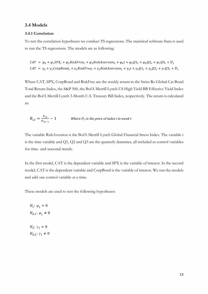
To test the correlation hypotheses we conduct TS regressions. The statistical software Stata is used

to run the TS regressions. The models are as following:

𝐶𝐴𝑇 = 𝜑0 + 𝜑1𝑆𝑃𝑋𝑡 + 𝜑2𝑅𝑖𝑠𝑘𝐹𝑟𝑒𝑒𝑡 + 𝜑3𝑅𝑖𝑠𝑘𝐴𝑣𝑒𝑟𝑠𝑖𝑜𝑛𝑡 + 𝜑4𝑡 + 𝜑5𝑄1𝑡 + 𝜑6𝑄2𝑡 + 𝜑7𝑄3𝑡 + 𝑈𝑡

𝐶𝐴𝑇 = 𝛾0 + 𝛾1𝐶𝑜𝑟𝑝𝐵𝑜𝑛𝑑𝑡 + 𝛾2𝑅𝑖𝑠𝑘𝐹𝑟𝑒𝑒𝑡 + 𝛾3𝑅𝑖𝑠𝑘𝐴𝑣𝑒𝑟𝑠𝑖𝑜𝑛𝑡 + 𝛾4𝑡 + 𝛾5𝑄1𝑡 + 𝛾6𝑄2𝑡 + 𝛾7𝑄3𝑡 + 𝑈𝑡

Where CAT, SPX, CorpBond and RiskFree are the weekly return in the Swiss Re Global Cat Bond

Total Return Index, the S&P 500, the BofA Merrill Lynch US High Yield BB Effective Yield Index

and the BofA Merrill Lynch 3-Month U.S. Treasury Bill Index, respectively. The return is calculated

as:

𝑅𝑖,𝑡 =𝑃𝑖,𝑡

𝑃𝑖,𝑡−1− 1 Where Pi,t is the price of index i in week t

The variable RiskAversion is the BofA Merrill Lynch Global Financial Stress Index. The variable t

is the time variable and Q1, Q2 and Q3 are the quarterly dummies, all included as control variables

for time- and seasonal trends.

In the first model, CAT is the dependent variable and SPX is the variable of interest. In the second

model, CAT is the dependent variable and CorpBond is the variable of interest. We run the models

and add one control variable at a time.

These models are used to test the following hypotheses:

𝐻1: 𝜑1 = 0

𝐻𝐴,1: 𝜑1 ≠ 0

𝐻2: 𝛾1 = 0

𝐻𝐴,2: 𝛾1 ≠ 0

14

3.4.2 Risk-adjusted return

We use Sharpe ratios to compare the risk-adjusted return across different asset classes. Sharpe ratio

is an industry standard to measure the “risk premium return earned per extra unit of total risk” (Reilly &

Brown, 2012, p. 965). In Andrew Lo’s article “The Statistics of Sharpe Ratios” from 2002, he suggests

two methods to calculate Sharpe ratio estimators and their statistical properties. In the first method

returns are assumed to be independently and identically distributed (IID). In the second, more

general method, this assumption is not made. The non-IID method incorporates phenomena such

as autocorrelation and heteroscedasticity, which are regularly observed in financial time series.

However, the non-IID method requires mathematics and statistics too advanced for this thesis.

Therefore, we use Lo’s first method and assume that returns are IID to derive the distribution and

the test statistic of the Sharpe ratio estimator. The second assumption we make is that there is no

covariance between the returns of the different indices and therefore no covariance between the

Sharpe ratio estimators. These assumptions and their potential weaknesses are further discussed in

the robustness section of the thesis.

The Sharpe ratio (SR) is defined as following:

𝑆𝑅 =𝜇 − 𝑅𝑓

𝜎

Where

𝜇 ≡ 𝐸[𝑅𝑡] 𝜎2 ≡ 𝑉𝑎𝑟(𝑅𝑡) 𝜎 = √𝜎2 𝑅𝑓 is the risk-free rate

To estimate the population parameters μ and σ we use the sample of historical returns (R1, R2, …

, RT) and compute the estimators:

�̂� =1

𝑇∑ 𝑅𝑡

𝑇𝑡=1 �̂� = √

1

𝑇∑ (𝑅𝑡 − �̂�)2𝑇

𝑡=1

We use μ̂ and σ̂ to compute the Sharpe ratio estimator:

𝑆�̂� =�̂� − 𝑅𝑓

�̂�

Using a large sample, due to the central limit theorem, the Sharpe ratio can be approximated by:

𝑆�̂�~𝑁(𝑆𝑅, 𝑉𝑎𝑟(𝑆�̂�))

15

Under the assumption that returns are IID, Lo (2002) shows that:

𝑉𝑎𝑟(𝑆�̂�) =1 +

12

𝑆𝑅2

𝑛

Where n is the number of observations

The difference of two sample means of normally distributed variables with no covariance has the

following variance:

𝑉𝑎𝑟(𝑆�̂�𝑥 − 𝑆�̂�𝑦) = 𝑉𝑎𝑟(𝑆�̂�𝑥) + 𝑉𝑎𝑟(𝑆�̂�𝑦) which gives:

𝑉𝑎𝑟(𝑆�̂�𝑥 − 𝑆�̂�𝑦) =1 +

12

𝑆𝑅𝑥2

𝑛𝑥+

1 +12

𝑆𝑅𝑦2

𝑛𝑦

The estimated variance and standard error of the Sharpe ratio estimator is then:

𝑉𝑎�̂�(𝑆�̂�𝑥 − 𝑆�̂�𝑦) =1 +

12

𝑆�̂�𝑥2

𝑛𝑥+

1 +12

𝑆�̂�𝑦2

𝑛𝑦

𝑆�̂�(𝑆�̂�𝑥 − 𝑆�̂�𝑦) = √1 +

12

𝑆�̂�𝑥2

𝑛𝑥+

1 +12

𝑆�̂�𝑦2

𝑛𝑦

The test statistic for SRx − SRy when Var(SRx) and Var(SRx) are unknown and cannot be assumed

equal is given by:

𝑡𝑑𝑓 =(𝑆�̂�𝑥−𝑆�̂�𝑦)−𝑑0

√1+

12

𝑆�̂�𝑥2

𝑛𝑥+

1+12

𝑆�̂�𝑦2

𝑛𝑦

𝑑𝑓 =((1+1

2𝑆�̂�𝑥

2) 𝑛𝑥⁄ +(1+1

2𝑆�̂�𝑦

2) 𝑛𝑦)⁄

2

((1+12

𝑆�̂�𝑥2

) 𝑛𝑥)⁄

2(𝑛𝑥−1)⁄ + (1+1

2𝑆�̂�𝑦

2) 𝑛𝑦)⁄

2

(𝑛𝑦−1)⁄

We use excel to manually compute the t-statistic and test the following hypotheses:

𝐻3 : 𝑆𝑅𝐶𝐴𝑇 − 𝑆𝑅𝑆𝑃𝑋 ≤ 0

𝐻𝐴,3: 𝑆𝑅𝐶𝐴𝑇 − 𝑆𝑅𝑆𝑃𝑋 > 0

𝐻4 : 𝑆𝑅𝐶𝐴𝑇 − 𝑆𝑅𝐶𝑜𝑟𝑝𝐵𝑜𝑛𝑑 ≤ 0

𝐻𝐴,4: 𝑆𝑅𝐶𝐴𝑇 − 𝑆𝑅𝐶𝑜𝑟𝑝𝐵𝑜𝑛𝑑 > 0

16

3.5 Descriptive statistics

This section displays descriptive statistics of the dependent and independent variables. Since these

summary statistic means are arithmetic, i.e. do not take compounding effects into account, they do

not allow us to draw conclusions about the compounded returns of the three markets but they give

an indication of the variables’ movement in the two periods.

Table 4. Descriptive statistics of the dependent variable, variables of interest and control variables of the crisis sample 2007.01.01-2009.12.31, where CAT is the weekly return of the Swiss Re Global Cat Bond TR Index, SPX is the weekly return of the S&P 500, CorpBond is the weekly return of the BofA ML High Yield Corporate Bond Index, RiskFree is the 3-month risk-free rate proxy and RiskAversion is the proxy for risk aversion based on the BofA ML GFSI.

VARIABLES Mean Std. Dev. Min Max

CAT 0.187 0.355 -2.440 1.339

SPX -0.079 3.602 -18.195 12.026

CorpBond 0.075 1.839 -10.862 5.499

RiskFree 0.047 0.052 -0.070 0.252

RiskAversion 0.679 1.005 -0.670 3.300

Table 5.

Descriptive statistics of the dependent variable, variables of interest and control variables of the post-crisis sample 2010.01.01-2017.03.31, where CAT is the weekly return of the Swiss Re Global Cat Bond TR Index, SPX is the weekly return of the S&P 500, CorpBond is the weekly return of the BofA ML High Yield Corporate Bond Index, RiskFree is the 3-month risk-free rate proxy and RiskAversion is the proxy for risk aversion based on the BofA ML GFSI.

VARIABLES Mean Std. Dev. Min Max

CAT 0.137 0.299 -2.463 1.735

SPX 0.215 1.972 -7.189 7.389

CorpBond 0.145 0.754 -2.833 3.088

RiskFree 0.002 0.006 -0.031 0.031

RiskAversion 0.149 0.371 -0.550 1.370

As we see in table 4, Cat bonds had the highest average return during the crisis period and a lower

standard deviation in this period than both equity and corporate bonds. In the post-crisis period,

shown in table 5, the equity- and corporate bond indices each have an average return that is higher

than that of the Cat bond index, but Cat bond returns still show the lowest volatility of the three.

The return of the risk-free rate shows higher volatility during the crisis period than during the post-

crisis period and has a much lower average return after the crisis. This is visualized in graph 2. In

graph 3 we see that equity- and corporate bond returns show noticeable volatility over the entire

period. The volatility of the risk aversion index can be seen in graph 1.

17

Graph 2. Weekly return of the BofA ML 3-Month U.S. Treasury Bill Index, 2007.01.01-2017.03.31.

Graph 3. Weekly return of the S&P 500 and the BofA ML US High Yield BB Effective Yield Index, 2007.01.01-2017.03.31.

-0,1

-0,1

0,0

0,1

0,1

0,2

0,2

0,3

0,3

2007 2008 2009 2010 2011 2012 2013 2014 2015 2016 2017

%

RiskFree

-20

-15

-10

-5

0

5

10

15

2007 2008 2009 2010 2011 2012 2013 2014 2015 2016 2017%

SPX CorpBond

18

4. Results

4.1 Correlation during the crisis

The results found from testing the correlation hypotheses in the crisis period are presented in table

6 and table 7. The results in table 6 allow us to reject H1 at a 10 % significance level when including

all control variables. This means we can show a positive correlation between Cat bond and equity

returns with a coefficient of 0.030. The results also show significance in the RiskAversion variable

and some explanatory power of a positive time trend. Comparing column (2) with column (3) to

(5) we find that when adjusting for risk aversion, the explanatory power of SPX on CAT decreases.

Table 6. Regression Cat bond- and equity market returns, 2007.01.01-2009.12.31. This table presents the test of H1 in the crisis period. CAT is the weekly return in the Swiss Re Global Cat Bond TR Index, SPX is the weekly return in the S&P 500, RiskFree is the 3-month risk-free rate proxy and RiskAversion is the proxy for risk aversion based on the BofA ML GFSI. The variable t is a weekly time variable and Q1, Q2 and Q3 are quarterly dummies.

(1) (2) (3) (4) (5)

VARIABLES CAT CAT CAT CAT CAT

SPX 0.030 0.035* 0.030* 0.030* 0.030*

(0.020) (0.020) (0.018) (0.017) (0.017)

RiskFree

1.233** 0.279 1.412 1.332

(0.580) (0.664) (0.897) (0.945)

RiskAversion

-0.084** -0.116*** -0.126**

(0.039) (0.044) (0.051)

t

0.002** 0.003**

(0.001) (0.001)

Q1

0.090

(0.075)

Q2

-0.036

(0.053)

Q3

0.047

(0.089)

Constant 0.189*** 0.139*** 0.241*** 0.025 -0.009

(0.027) (0.045) (0.052) (0.116) (0.147)

Observations 155 146 146 146 146

R-squared 0.095 0.134 0.170 0.204 0.220

Prob > F 0.020**

Robust standard errors in parentheses

*** p<0.01, ** p<0.05, * p<0.1

19

Table 7. Regression Cat bond- and corporate bond market returns, 2007.01.01-2009.12.31. This table presents the test of H2 in the crisis period. CAT is the weekly return in the Swiss Re Global Cat Bond TR Index, CorpBond is the weekly return in the BofA ML High Yield Corporate Bond Index, RiskFree is the 3-month risk-free rate proxy and RiskAversion is the proxy for risk aversion based on the BofA ML GFSI. The variable t is a weekly time variable and Q1, Q2 and Q3 are quarterly dummies.

(6) (7) (8) (9) (10)

VARIABLES CAT CAT CAT CAT CAT

CorpBond 0.088** 0.096** 0.087** 0.084** 0.085**

(0.042) (0.041) (0.038) (0.038) (0.037)

RiskFree

1.480** 0.749 1.508 1.328

(0.601) (0.747) (0.972) (0.995)

RiskAversion

-0.063* -0.088*** -0.095**

(0.034) (0.034) (0.039)

t

0.002* 0.002

(0.001) (0.001)

Q1

0.007

(0.054)

Q2

-0.098*

(0.055)

Q3

0.023

(0.090)

Constant 0.185*** 0.115** 0.194*** 0.044 0.082

(0.029) (0.047) (0.057) (0.115) (0.132)

Observations 146 146 146 146 146

R-squared 0.197 0.240 0.260 0.277 0.292

Prob > F 0.016**

Robust standard errors in parentheses

*** p<0.01, ** p<0.05, * p<0.1

The results in table 7 are stronger than the results in the previous regression and allow us to reject

H2 that Cat bond returns are not correlated with returns at the corporate bond market at a 5%

significance level. The variable of interest CorpBond has an explanatory power of the dependent

variable CAT and that the correlation is positive with a coefficient of 0.085. Comparing the results

in column (7) with column (8) to (10) we find that the explanatory power of corporate bond market

returns on Cat bond returns decrease when controlling for risk aversion. We also find that there is

no longer significance in the controlling variable RiskFree when also controlling for risk aversion.

This is the case when testing both H1 and H2.

20

4.2 Correlation after the crisis

Table 8 presents the results found from testing H1 that Cat bond returns are not correlated with

equity returns, in the post-crisis period. As we see in the table there is no significance in the SPX

variable and therefore we cannot reject the null hypothesis. These results from the post-crisis

period support the claim that there is no proof of a significant correlation between the Cat bond-

and the equity market.

Table 8. Regression Cat bond- and equity market returns, 2010.01.01-2017.03.31. This table presents the test of H1 in the post-crisis period. CAT is the weekly return in the Swiss Re Global Cat Bond TR Index, SPX is the weekly return in the S&P 500, RiskFree is the 3-month risk-free rate proxy and RiskAversion is the proxy for risk aversion based on the BofA ML GFSI. The variable t is a weekly time variable and Q1, Q2 and Q3 are quarterly dummies.

(1) (2) (3) (4) (5)

VARIABLES CAT CAT CAT CAT CAT

SPX -0.007 -0.007 -0.007 -0.007 -0.006 (0.009) (0.009) (0.009) (0.009) (0.010)

RiskFree

-1.148 -1.148 -0.444 -0.335 (2.331) (2.378) (2.543) (2.606)

RiskAversion

-1.86e-05 -0.024 -0.031 (0.043) (0.047) (0.048)

t

-2.18e-04 -2.29e-04 (0.000) (0.000)

Q1

-0.015 (0.053)

Q2

-0.014 (0.051)

Q3

0.153*** (0.054)

Constant 0.139*** 0.142*** 0.142*** 0.191*** 0.161*** (0.015) (0.015) (0.015) (0.044) (0.061)

Observations 379 358 358 358 358

R-squared 0.002 0.002 0.002 0.007 0.062

Prob > F 0.000***

Robust standard errors in parentheses

*** p<0.01, ** p<0.05, * p<0.1

21

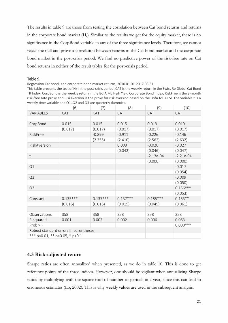
The results in table 9 are those from testing the correlation between Cat bond returns and returns

in the corporate bond market (H2). Similar to the results we get for the equity market, there is no

significance in the CorpBond variable in any of the three significance levels. Therefore, we cannot

reject the null and prove a correlation between returns in the Cat bond market and the corporate

bond market in the post-crisis period. We find no predictive power of the risk-free rate on Cat

bond returns in neither of the result tables for the post-crisis period.

Table 9. Regression Cat bond- and corporate bond market returns, 2010.01.01-2017.03.31. This table presents the test of H2 in the post-crisis period. CAT is the weekly return in the Swiss Re Global Cat Bond TR Index, CorpBond is the weekly return in the BofA ML High Yield Corporate Bond Index, RiskFree is the 3-month risk-free rate proxy and RiskAversion is the proxy for risk aversion based on the BofA ML GFSI. The variable t is a weekly time variable and Q1, Q2 and Q3 are quarterly dummies.

(6) (7) (8) (9) (10)

VARIABLES CAT CAT CAT CAT CAT

CorpBond 0.015 0.015 0.015 0.013 0.019 (0.017) (0.017) (0.017) (0.017) (0.017)

RiskFree

-0.899 -0.911 -0.226 -0.146 (2.355) (2.410) (2.562) (2.632)

RiskAversion

0.003 -0.020 -0.027 (0.042) (0.046) (0.047)

t

-2.13e-04 -2.21e-04 (0.000) (0.000)

Q1

-0.017 (0.054)

Q2

-0.009 (0.050)

Q3

0.156*** (0.053)

Constant 0.135*** 0.137*** 0.137*** 0.185*** 0.153** (0.016) (0.016) (0.015) (0.045) (0.061)

Observations 358 358 358 358 358

R-squared 0.001 0.002 0.002 0.006 0.063

Prob > F 0.000***

Robust standard errors in parentheses

*** p<0.01, ** p<0.05, * p<0.1

4.3 Risk-adjusted return

Sharpe ratios are often annualized when presented, as we do in table 10. This is done to get

reference points of the three indices. However, one should be vigilant when annualizing Sharpe

ratios by multiplying with the square root of number of periods in a year, since this can lead to

erroneous estimates (Lo, 2002). This is why weekly values are used in the subsequent analysis.

22

As shown in table 10, the annualized risk-adjusted return has been higher for Cat bonds than for

equity and corporate bonds. This is true for all three periods.

Tables 11-13 show the results from conducting difference of means t-test of the Sharpe ratios to

determine whether risk-adjusted return has been significantly higher in the Cat bond market than

the markets for the two other asset classes. For the crisis period we get a difference of means in

weekly risk-adjusted return between CAT and SPX of 0.48 and between CAT and CorpBond of

0.41. The differences are significant at a 1% level. We reject the null hypotheses H3 and H4 in the

crisis period and conclude that the risk-adjusted return in the Cat bond market has been higher

than those of the equity- and corporate bond markets.

Table 10. Annualized Sharpe ratio per market. This table presents the annualized1 Sharpe ratios for the crisis period 2007.01.01-2009.12.31, post-crisis period 2010.01.01-2017.03.31 and over the total period (crisis and post-crisis). CAT, SPX and CorpBond are the Sharpe ratios based on weekly returns of the Swiss Re Global Cat Bond TR Index, the S&P 500 and the BofA ML High Yield Corporate Bond Index, respectively.

VARIABLES CAT SPX CorpBond

Crisis 2.875 -0.400 0.110

Post-crisis 3.183 0.739 1.361

Total period 3.064 0.236 0.670 1 The Sharpe ratios have been annualized using weekly Sharpe Ratios × √52

Table 11. Sharpe ratios difference of means, t-test, 2007.01.01-2009.12.31. This table presents the difference of means t-test of Sharpe ratios for the crisis period. μ̂ is the sample mean of weekly returns and σ̂ is the standard deviation of weekly returns of the Swiss Re Global Cat Bond TR Index, the S&P 500 and the BofA ML High Yield Corporate Bond Index. RiskFree is the 3-month risk-free rate proxy, Var̂(SR̂) is the variance of the Sharpe ratio sample mean and SE(̂SR̂) is the standard error of the Sharpe ratio sample mean. The variables diff CAT SPX and diff CAT CorpBond are the difference of means.

VARIABLES CAT SPX CorpBond RiskFree diff CAT SPX diff CAT CorpBond

# of observations 146 146 146 146 146 146

�̂� return % 0.191 -0.157 0.075 0.047

�̂� return % 0.362 3.665 1.833

Sharpe ratio 0.399 -0.055 0.015

0.480*** 0.410***

𝐕𝐚𝐫(̂𝐒�̂�) 0.007 0.007 0.007

0.009 0.009

𝐒𝐄(̂𝐒�̂�) 0.095 0.095

t-statistic

5.057 4.315

df

290 290

*** p<0.01, ** p<0.05, * p<0.1

23

Table 12. Sharpe ratios difference of means, t-test, 2010.01.01-2017.03.31. This table presents the difference of means t-test of Sharpe ratios for the post-crisis period. μ̂ is the sample mean of weekly returns and σ̂ is the standard deviation of weekly returns of the Swiss Re Global Cat Bond TR Index, the S&P 500 and the BofA ML High Yield Corporate Bond Index. RiskFree is the 3-month risk-free rate proxy, Var(̂SR̂) is the variance of the Sharpe ratio sample mean and SE(̂SR̂) is the standard error of the Sharpe ratio sample mean. The variables diff CAT SPX and diff CAT CorpBond are the difference of means.

VARIABLES CAT SPX CorpBond RiskFree diff CAT SPX

diff CAT CorpBond

# of observations 358 358 358 358 358 358

�̂� return % 0.137 0.204 0.145 0.002

�̂� return % 0.306 1.969 0.753

Sharpe ratio 0.441 0.102 0.189

0.322*** 0.236***

𝐕𝐚𝐫(̂𝐒�̂�) 0.003 0.003 0.003

0.005 0.005

𝐒𝐄(̂𝐒�̂�) 0.071 0.071

t-statistic

4.573 3.337

df

713 713

*** p<0.01, ** p<0.05, * p<0.1

Table 12 shows the results found from testing the risk-adjusted return hypotheses in the post-crisis

period. The difference of means in weekly risk-adjusted return between the Cat bond market and

the equity market is 0.322. For the Cat bond and the corporate bond market the difference is

somewhat lower, at 0.236. Similar to the crisis period, the results are significant at a 1% level and

allow us to reject H3 and H4. Thus, risk-adjusted return in the Cat bond market has been higher

than those of the equity- and corporate bond market in the post-crisis period.

Lastly, we present the results found from testing the entire period from January 2007 until March

2017 in table 13. We find that the difference in risk-adjusted return in the Cat bond market

compared to the stock market is 0.322 whereas the difference between the Cat bond- and the

corporate bond market is 0.236. The results show significantly higher risk-adjusted return in the

Cat bond market at a 1% level and allow us to reject both H3 and H4. For the entire period we

conclude that risk-adjusted return has been higher in the Cat bond market compared to the markets

of the two other asset classes.

24

Table 13. Sharpe ratios difference of means, t-test, 2007.01.01-2017-03-31. This table presents the difference of means t-test of Sharpe ratios for the total period. μ̂ is the sample mean of weekly returns and σ̂ is the standard deviation of weekly returns of the Swiss Re Global Cat Bond TR Index, the S&P 500 and the BofA ML High Yield Corporate Bond Index. RiskFree is the 3-month risk-free rate proxy, Var(̂SR̂) is the variance of the Sharpe ratio sample mean and SE(̂SR̂) is the standard error of the Sharpe ratio sample mean. The variables diff CAT SPX and diff CAT CorpBond are the difference of means.

VARIABLES CAT SPX CorpBond RiskFree diff CAT SPX diff CAT CorpBond

# of observations 504 504 504 504 504 504

μ̂ return % 0.153 0.100 0.124 0.015

σ̂ return % 0.324 2.583 1.173

Sharpe ratio 0.425 0.033 0.093

0.392*** 0.332***

Var(̂SR̂) 0.002 0.002 0.002

0.004 0.004

SE(̂SR̂) 0.064 0.065

t-statistic

6.090 5.150

df

1004 1004

*** p<0.01, ** p<0.05, * p<0.1

5. Analysis

In this section we analyze each time period separately and look at both correlation and risk-adjusted

return results to discuss the value of Cat bonds for investors.

5.1 Crisis period 2007-2009

In line with previous research by Cummins & Weiss (2009) and Gürtler, Hibbeln & Winkelvos

(2016) we find a significant correlation (beta) between returns in the Cat bond market and the

equity- as well as the corporate bond market during the crisis period. Even so, the predictive power

of returns in the equity- or corporate bond market on Cat bond returns is low. When we test the

correlation with the equity market it generates a beta of approximately 0.03, and when testing

against the corporate bond market the beta is approximately 0.09. The idea of Cat bonds as zero-

beta assets is proven to be untrue during the crisis, but the low betas still suggest that Cat bonds

have a very low systematic risk and therefore are beneficial for diversification.

Some of the Cat bonds outstanding during the crisis went into default when Lehman Brothers

declared bankruptcy in 2008 and Gürtler, Hibbeln & Winkelvos (2016) have proven that the

bankruptcy had an effect on Cat bond returns. Therefore, we suspect that some of the correlation

is caused by the default of these bonds due to the swap counterparty and not due to the market

decline. The restrictions implemented after this event described by Wattman & Fieg (2008) might

in the case of future crises, generate even lower betas of Cat bonds.

25

When including a proxy for risk aversion in the model the results display lower betas. These

findings suggest that some of the correlation with the equity- and corporate bond market can be

explained by changes in attitudes towards risk during a period of crisis. Shown by the risk aversion

index that we have used as a proxy in the models, investors’ risk aversion increased during the

crisis. Our expectation is that when the level of risk aversion increases, investors require a higher

premium for taking on more risk in all parts of the capital market. This would affect returns on the

equity-, corporate bond- and Cat bond markets negatively and the correlation between the different

markets increases. These expectations are confirmed by the results and the findings allow us to

statistically show what previously has been theoretically discussed by Bantwal & Kunreuther (2000)

about the effect of risk aversion on Cat bond premiums.

The correlation between Cat bond- and corporate bond returns is higher than that of Cat bond-

and equity returns. This result is not surprising and can be explained by the fact that Cat bonds and

corporate bonds are both debt instruments, have similar ratings and the investors of the two

instruments might have similar behavior. Cat bonds are initially issued to QIBs and are traded in

large denominations, which are features we connect to the debt market rather than the equity

market.

We would expect the risk-free rate to have relatively high and significant correlation with Cat bond

returns in the model because Cat bonds are priced above a floating risk-free rate. This is supported

by our findings before we include a proxy for risk aversion, which, when included, removes the

significance of the risk-free rate proxy. A possible explanation for this is multicollinearity, since the

variables for risk-free rate and risk aversion are negatively correlated during the crisis (table 14).

Table 14. Correlation matrix, 3-month risk-free rate proxy and risk aversion proxy, 2007.01.01-2009-12-31.

RiskFree RiskAversion

RiskFree 1.00

RiskAversion -0.54*** 1.00

*** p<0.01, ** p<0.05, * p<0.1

In addition to the low systematic risk, Cat bonds have outperformed both the equity- and corporate

bond market, measured by risk-adjusted return during the crisis. The annualized Sharpe ratio for

Cat bonds in the crisis period is 2.88 compared to -0.40 for equity and 0.11 for high yield corporate

bonds and the weekly risk-adjusted returns are proven significantly higher for Cat bonds. This

might be explained by the previous results concerning the correlation; the low beta gives a lower

effect on Cat bond returns when the market fell during the crisis – the returns stay on a relatively

26

high level and the volatility does not rise to the levels shown in the rest of the market. Our findings

support the conclusion drawn by Kish (2016) that the risk incurred by investing in Cat bonds might

to some extent be offset by the high returns.

Thus, for the crisis period we find low systematic risk and higher risk-adjusted returns in

comparison to the other assets. Consequently, Cat bonds can be presented as valuable securities

for diversification in a period of crisis and might be even more valuable in case of a future crisis

because of the lessons learned and improvements made in the Cat bond market since the last one.

5.2 Post-crisis period 2010-2017

In the post-crisis period we do not get any significant results when testing the correlation

hypotheses. This means that we cannot find any proof of correlation between Cat bond returns

and neither stock- nor corporate bond returns. This is in agreement with previous results presented

by Cummins & Weiss (2009) and Kish (2016) and supports our expectations that Cat bond returns

are determined by the risk of natural disasters (i.e. their default risk) and not fluctuations in capital

markets.

The expectation that Cat bonds are zero-beta assets is based on the idea of rational behavior of

investors. On the contrary, Bantwal & Kunreuther (2000) suggest in their paper that investors are

not completely rational when it comes to Cat bonds and that different biases affect the premiums,

such as ambiguity aversion, loss aversion and risk aversion; even though the authors maintain the

claim that Cat bonds are uncorrelated with the rest of the market. If risk aversion would be a

determining factor in Cat bond premiums we would expect the coefficient to be negative and

significant, but we find no explanatory power by the risk aversion proxy of Cat bond returns in the

period after the crisis. The results therefore oppose the theoretical explanation made by Bantwal

& Kunreuther (2000) that level of risk appetite in the market has an effect on investors’ required

premium for Cat bonds. The level of loss aversion should also be partly reflected in the risk

aversion proxy because the index is calculated from both very risky assets and less risky assets.

Other possible biases mentioned by Bantwal & Kunreuther (2000) such as ambiguity aversion due

to investors’ uncertainty about natural disasters are less likely to be captured by the risk aversion

proxy and might still have an effect on premiums required.

27

As mentioned earlier, we expect the risk-free rate to be correlated with the Cat bond returns

because of the pricing structure of Cat bonds. This is not in line with our findings for the post-

crisis period and this can be explained by the low volatility in the risk-free rate after the crisis. The

rationale of this explanation is that we find a correlation when the volatility is higher (during the

crisis) but not when the volatility is low (post-crisis).

During the period from 2010 to the first quarter of 2017, the weekly average return of Cat bonds

is lower than the return of both the equity- and corporate bond market. The mean return of Cat

bonds is also lower than the return observed during the crisis. Generally, when a market grows and

matures, it becomes more effective and the returns decline. As described by Wattman & Fieg

(2008), the Cat bond market has become more standardized: the bonds are rated and the risks are

now more isolated to the occurrence of natural disasters. These changes in combination with the

performance during the crisis might be the reason for the increased attractiveness of Cat bonds,

which we see in the continued growth of the market, and could explain why Cat bond returns are

lower in the post-crisis period. Looking at the risk-adjusted returns however, we see that Cat bonds

have outperformed both the stock market and the high yield corporate bond market. This is

because of the low volatility of Cat bond returns relative to the volatility of stocks and corporate

bonds. Again, this is the result of the low systematic risk that Cat bonds show after the crisis. The

low volatility can also be connected to the reduced exogenous- and modelling risks due to

standardization in the market.

The market after the crisis is known for very low interest rates, a phenomenon widely discussed by

researchers. Cat bonds have a credit risk but because of their structure, with the floating interest

rate as a base, the duration risk is low. According to Alloway (2016), this would suggest that

investors in the low interest rate environment will turn away from Cat bonds and into other assets

with longer maturity and thereby higher duration risks. This is the opposite of our findings when

observing the Cat bond market in the low interest environment.

Similar to the crisis period, we find Cat bonds have been valuable assets to investors after the crisis,

considering their low correlation with other markets. Even though the differences in Sharpe ratios

are less pronounced during the post-crisis period, Cat bonds have clearly out-perform the stock

market and the high yield segment of the corporate bond market.

28

5.3 Risk-adjusted return total period 2007-2017

We examine the total period to see how well Cat bonds have performed in different market

environments. Observing the results, we find that Cat bonds’ risk-adjusted return has been

significantly higher than those of stocks and corporate bonds. The mean weekly return has been

higher and the volatility has been lower in comparison to the other asset classes tested. These clear

differences can be explained by the fact that Cat bonds were less affected by the crisis. This further

strengthens the previous inferences that Cat bonds add value to an investor and that this is

consistent in differing market conditions, even over a longer period of time.

6. Future research

The methods we have chosen to test the hypotheses is TS regressions and difference of means

tests. An alternative approach to test if Cat bonds are a good instrument for diversification could

be to synthesize two different portfolios with only one including Cat bonds and compare the two.

This method calls for a more detailed dataset with information about individual Cat bonds that we

do not have access to since Cat bonds are traded OTC. Using indices as proxies, we find the

method chosen in this thesis more appropriate. If more detailed data would be obtained, the model

could be developed even further.

Access to more detailed data about Cat bonds would also allow for future researchers to examine

the different factors that impact Cat bond premiums. Kish (2016) provides input to the research

by listing risks that might influence the required return and Bantwal & Kunreuther (2000) discuss

biases that might affect the premiums. Both these papers have a theoretical rather than an empirical

approach. An interesting empirical approach for future researchers could be to build a model that

explains the effect of the different risks and biases on Cat bond premiums.

7. Robustness

7.1 Endogeneity and causality

The data we have of the Swiss Re Global Cat Bond TR Index does not contain information about

the liquidity of the bonds traded within the index. This gives rise to a possible omitted variable

problem, since investors demand higher premiums for illiquid assets. However, considering the

size of the Cat bond market in comparison with the equity and corporate bond market, the liquidity

of Cat bonds is unlikely to influence the returns in the other markets and we therefore believe that

the estimates are unlikely to be biased because of this.

29

In the TS regression models we include a proxy for risk aversion based on an index to reduce

possible endogeneity issues caused by the level of risk aversion in the market. There are two

concerns about using this index as a proxy. First, in previous research, Bantwal & Kunreuther

(2000) discuss the potential effect of other psychological factors such as ambiguity aversion, due

to the lack of knowledge about Cat bonds and the uncertainty in modelling natural disaster, on Cat

bond premiums. It is unlikely that the risk aversion proxy captures these imperfections, but since

they do not directly alter the market returns of stocks and corporate bonds this should not give

rise to an endogeneity problem. Second, the utility functions of investors are unobservable, which

makes their risk aversion difficult to quantify and it is difficult to tell how well the index captures

the true level of risk aversion. If the proxy cannot perfectly track the risk aversion, this still induces

a possible endogeneity problem. A way of investigating this would be to extend the method with

models involving different ways of measuring risk appetite.

Throughout this thesis we are interested in finding a correlation between the dependent variable

and variables of interest and the method chosen does not allow us to make any conclusions about

causality. Previous research by Wang & Kutan (2013) has shown that natural disasters do not have

significant impact on the equity market. We do not test this hypothesis or include variables for

natural disasters in the models and because of this we cannot make any statements about causal

effects. It is not in our objective to draw conclusions about causality since our main interest is to

examine the beta of Cat bonds.

In both the regression models for the post-crisis period, the R-squared is approximately 0.06. This

is not considered as an issue since Cat bond returns mainly are determined by the probability of

the bond being triggered (i.e. the probability of the disaster occurring) and other Cat bond

characteristics such as modelling risks and initial costs of education.

7.2 Risk-free rate proxy

As a proxy for the risk-free rate we use the return of the BofA Merrill Lynch 3-Month U.S. Treasury

Bill Index, which is based on the three-month U.S. treasury floating rate. For the period of the

crisis, the results are in line with our expectation that the risk-free rate has an explanatory power

on Cat bond returns. During this period there is sufficient volatility of the variable. For the period

after the crisis the volatility of risk-free return is low and this is most likely the explanation to why

the coefficient of the risk-free rate variable is not significant, which is in contrast to our

expectations. To check the robustness of the risk-free rate proxy we test if the results differ when

using the risk-free yield of a different index, US Generic Government 3-month yield (Bloomberg

30

ticker: USGG3M), but get no significance in this case either. We also test if we find a correlation

when using prices of the BofA Merrill Lynch 3-Month U.S. Treasury Bill Index instead of returns

but the results are unchanged.

7.3 Sharpe ratio

One weakness in the Sharpe ratio computations is the simplifying assumption that returns are IID.

It is highly likely that this assumption is violated by the financial time series we are studying due to

autocorrelation and volatility clustering. Lo (2002) argues that ignoring these factors can lead to

estimate errors. Still, this assumption is crucial in order for us to be able to test the significance of

the results. Using our method, the differences in Sharpe ratios are very substantial, all significant at

a 0.05% level, suggesting that the results would still hold even if the estimators to some degree are

biased.

The other assumption we make is that the covariance between the Sharpe ratios is zero. Since we

find little or no correlation (and consequently little or no covariance) in returns between Cat bonds

and the other assets, the covariance of Sharpe ratios should not affect the results in a meaningful

way. In addition, the significant betas we find are positive, meaning that the covariance is positive.

This would increase the t-statistics, since the variance of the difference of means decreases with

increased covariance.1 Hence, we can safely make the assumption that there is no covariance

between the Sharpe ratios.

The excess return of the S&P 500 (the return of the S&P 500 minus the risk-free return) during

the crisis is negative, making the Sharpe ratio negative. Comparing positive and negative Sharpe

ratios is somewhat problematic. Consider two different portfolios, A and B, with equal negative

excess returns. If A has higher standard deviation, it will show a higher (less negative) Sharpe ratio

and would seem like a more attractive investment. However, choosing between two portfolios with

equal returns and different standard deviations, the best option is the portfolio with the lowest

standard deviation, in this case B. In other words, the high volatility of the S&P 500 during the

crisis increases the Sharpe ratio instead of lowering it. Since the results already allow us to reject

the null at the 1% significance level, this has no effect on our findings.

1 Since for dependent variables, Var(X − Y) = Var(X) + Var(Y) − 2Cov(X, Y)

31

8. Conclusion

Cat bonds offer vital protection to insurance companies by giving them access to reinsurance

through the capital market. These instruments are often described as zero-beta assets in the

literature. The rationale behind this is that the state of the economy has no influence on the

likelihood of a natural disaster and that even large natural disasters have insignificant effect on the

financial market. Our research demonstrates a significant correlation with the equity- as well as

high yield corporate bond market during the subprime crisis. Thus, it allows us to disprove that

Cat bonds are zero-beta instruments in such extreme market conditions. The results we present in

this thesis indicate that this correlation between Cat bond returns and equity- and corporate bond

returns partly can be explained by the investors’ risk aversion during a financial crisis - a

contribution to the behavioral aspect of Cat bond returns previously discussed by researchers but

never statistically tested.

Nevertheless, supported by the low betas during the crisis, we suggest that Cat bonds still offer a

relevant source of diversification. In addition to this we argue that improvements made in the Cat

bond market after the subprime crisis might lower the correlation with the market in case of a

similar event in the future. When further examining betas after the crisis we find no evidence of

correlation between Cat bond returns and equity- or high yield corporate bond returns. This

strengthens the argument that Cat bonds offer diversification to investors.

Moreover, when comparing the performance of the Cat bond market with the equity- and high

yield corporate bond market by looking at weekly Sharpe ratios, thereby taking into account the

systematic- as well as the idiosyncratic risk, we find that Cat bonds clearly have out-performed the

two other asset classes. Cat bonds have a significantly higher risk-adjusted return during the crisis

and post-crisis period. The high risk-adjusted returns of Cat bonds can be attributed to the low

systematic risk of these instruments, which made them resilient to the market crash in 2007-2008.

After the crisis the volatility of Cat bonds remains low, yielding a higher risk-adjusted return than

those of stocks and high yield corporate bonds. Again, the low volatility can be explained by the

low systematic risk and the structural improvements made in the Cat bond market.

Analyzing the correlation and risk-adjusted returns over the last 10 years we find some important

insights of the continuously growing Cat bond market during and after a financial crisis. Not only

do Cat bonds offer value to the insurance market, but as our research demonstrates, Cat bonds are

low-beta instruments with high risk-adjusted return that also offer value to investors.

32

References

Alloway, T. (2016) Three things that show investors are making a huge bet on low interest rates.

Retrieved 2017-04-12 from https://www.bloomberg.com/news/articles/2016-07-28/three-

things-that-show-investors-are-making-a-huge-bet-on-low-interest-rates

ARTEMIS. (2012). The shape of catastrophe bond price seasonality. Retrieved 2017-04-10 from

http://www.artemis.bm/blog/2012/10/22/the-shape-of-catastrophe-bond-price-seasonality/.

ARTEMIS. (2017). Catastrophe bond & ILS capital issued & outstanding by year. Retrieved 2017-

02-23 from

http://www.artemis.bm/deal_directory/cat_bonds_ils_issued_outstanding.html.

Bantwal, V. J., & Kunreuther, H. C. (2000) A Cat Bond Premium Puzzle? Journal of Psychology

and Financial Markets, 1(1). 76-99.

Barrieu, P., & Loubergé, H. (2009) Hybrid Cat Bonds. Journal of Risk and Insurance, 76(3), 547-

578.

Berk, J., & DeMarzo, P. (2011) Corporate Finance. (2. ed.) Edinburgh: Pearson Education Limited.

Cummins, J. D. (2008) CAT Bonds and Other Risk-Linked Securities: State of the Market and

Recent Developments. Risk Management and Insurance Review, 11(1), 23-47.

Cummins, J. D., & Weiss, M. A. (2009). Converge of Insurance and Financial Markets: Hybrid and

Securitized Risk-Transfer Solutions. The Journal of Risk and Insurance, 76(3), 493-545.

FINRA (Financial Industry Regulatory Authority). (2013). Catastrophe Bonds and Other Event-

Linked Securities. Retrieved 2017-02-17 from

http://www.finra.org/investors/alerts/catastrophe-bonds-and-other-event-linked-securities.

Froot, K. A. (2001). The Market for Catastrophe Risk: A Clinical Examination. Journal of Financial

Economics, 60(2-3), 529-571.

Gürtler, M., Hibbeln, M., & Winkelvos, C. (2016). The Impact of the Financial Crisis and Natural

Catastrophes on CAT Bonds. The Journal of Risk and Insurance, 83(3), 579-612.

Kish, R. J. (2016) Catastrophe (CAT) bonds: risk offsets with diversification and high returns.

Financial Services Review, 25(3), 303-329.

Lo, A. W. (2002). The Statistic of Sharpe Ratios. Financial Analysts Journal, 58(4), 36-52.

33

Reilly, F. K., & Brown, K. C. (2012). Investment Analysis & Portfolio Management. (10. ed.)

Mason, Ohio: South-Western Cengage Learning.

Reuters. (2010) BofA Merrill launches Global Financial Stress Index. Retrieved 2017-04-10 from

http://www.reuters.com/article/markets-stressindex-idUSN2920764420101129.

Swiss Re. (2012). What are Insurance Linked Securities (ILS), and Why Should they be Considered?

(Presentation to the CANE Fall Meeting, September 2012). Retrieved from

http://www.casact.org/community/affiliates/CANE/0912/Cat-Bond.pdf.

Swiss Re. (2014). Swiss Re Cat Bond Indices Methodology. (Expertise Publication). Retrieved from

http://www.swissre.com/library/Swiss_Re_Cat_Bond_Indices_Methodology.html

Wang, L., & Kutan, A. M. (2013). The Impact of Natural Disasters on Stock Markets: Evidence

from Japan and the US. Comparative Economic Studies, 55, 672-686.

Wattman, M. P., & Feig, M. (2008). The Credit Crisis and Insurance-Linked Securities: No

catastrophe for Catastrophe bonds. The Journal of Structured Finance, 14(3), 80-85.