CENTRAL POINTS AND APPROXIMATION IN RESIDUATED LATTICES

PROCEEDINGS OF THEAMERICAN MATHEMATICAL SOCIETYVolume 00, Number 0, Pages 000–000S 0002-9939(XX)0000-0

CENTRAL POINTS AND APPROXIMATION IN RESIDUATED

LATTICES

RADIM BELOHLAVEK AND MICHAL KRUPKA

Abstract. The paper presents results on approximation in residuated lattices

given that closeness is assessed by means of biresiduum. We describe centralpoints and optimal central points of subsets of residuated lattices and provide

properties of these points. In addition, we present algorithms for two problems

regarding optimal approximation.

1. Introduction and preliminaries

Suppose there is a picture with two poles with lengths ≤ 1. If we do not knowthe magnification factor of the picture, an obvious way to define a similarity s1,2 ofthe two poles is to measure their lengths a1 and a2 in the picture and put

(1.1) s1,2 = min

(a1a2

,a2a1

),

because it is independent of the magnification factor of the picture, i.e., s1,2 =

min(

c·a1

c·a2, c·a2

c·a1

)for every c > 0. A “central pole”, i.e., a pole equally similar to

each of the poles, then has the length

(1.2) l =√a1 ·√a2.

If, however, the magnification factor is known, we may obtain the actual lengthsa1 and a2 of the poles and set

(1.3) s1,2 = 1− |a1 − a2|.In this case, the length a of the “central pole” is

(1.4) a =a1 + a2

2.

Clearly, for a collection of poles with lengths ai, the length of the central poles fors1,2 given by (1.1) and (1.3) is

a =√

mini

ai ·√

maxi

ai and a =mini ai + maxi ai

2,

respectively.The above considerations may be carried over to a general setting of approxima-

tion in complete residuated lattices [1, 8], i.e., structures L = 〈L,⊗,→,∧,∨, 0, 1〉such that 〈L,∧,∨, 0, 1〉 is a complete lattice, 〈L,⊗, 1〉 is a commutative monoid,and ⊗ (multiplication) and → (residuum) form an adjoint pair, i.e., a ⊗ b ≤ c iff

2000 Mathematics Subject Classification. Primary 54C40, 14E20; Secondary 46E25, 20C20.

Key words and phrases. Residuated lattice, central point.

c©XXXX American Mathematical Society

1

2 RADIM BELOHLAVEK AND MICHAL KRUPKA

a ≤ b → c. In what follows, we use the following three well-known examples ofcomplete residuated lattices on L = [0, 1] induced by continuous t-norms [7]: stan-dard Lukasiewicz algebra (a ⊗ b = max(0, a + b − 1), a → b = min(1, 1 − a + b)),standard Goguen algebra (a ⊗ b = a · b, a → b = 1 if a ≤ b, and a → b = b/aotherwise), standard Godel algebra (a ⊗ b = min(a, b), a → b = 1 if a ≤ b, anda→ b = b otherwise). One may easily check that in (1.1),

(1.5) s1,2 = a1 ↔ a2

with ↔ being the biresiduum corresponding to the standard Goguen algebra andthat in (1.2),

(1.6) a = (a1 ∧ a2)⊗√a1 ↔ a2,

with√

denoting the square root of ⊗ (see [5] and Section 3). Likewise, (1.5) and

(1.6) become (1.3) and (1.4) if ↔ and ⊗ are the biresiduum and t-norm of thestandard Lukasiewicz algebra.

It is well known [4] that a biresiduum ↔, defined in any residuated lattice bya↔ b = (a→ b) ∧ (b→ a), satisfies

a↔ b = 1 iff a = b,(1.7)

a↔ b = b↔ a,(1.8)

(a↔ b)⊗ (b↔ c) ≤ a↔ c.(1.9)

Hence, a↔ b may be interpreted as an element in L representing similarity (close-ness) of a and b. Note also that (1.7)–(1.9) resemble dual versions of the ax-ioms of a metric with a generalized triangular inequality. Indeed, for the standard Lukasiewicz algebra, d↔(a, b) = 1− (a↔ b) is a [0, 1]-valued metric on [0, 1] (moregenerally, using d↔(a, b) = f(a ↔ b) one obtains a metric from a biresiduum of acontinuous Archimedean t-norm with an additive generator f [7]). For the standardGodel algebra, in which case the t-norm is not Archimedean, d↔(a, b) = 1−(a↔ b)is a [0, 1]-valued ultrametric on [0, 1]. Note also that residuated lattices and theirgeneralizations, developed initially within the studies of ring ideals [8] and sincethen studied within partially ordered algebraic structures [6], are the main struc-tures of truth degrees used in many-valued logic [2, 3, 4] in which biresiduum is thetruth function of the connective of equivalence.

In this paper, we present results motivated by the following problem, alluded toby the initial example. Given a set of elements of a residuated lattice, what areits central points, i.e., elements which are similar (as much as possible or to somespecified similarity level) to every element of the set, provided similarity is assessedby means of biresiduum?

We assume familiarity with basic properties of residuated lattices and basicconcepts from tolerance relations, i.e., reflexive and symmetric binary relations.A block of a tolerance T on a set U is a subset B of U for which B × B ⊆ T .A maximal block of T is a block B of T which is maximal with respect to set inclu-sion. A collection of maximal tolerance blocks of T is denoted by U/T and forms acovering of U . A class of T given by u ∈ U is the set [u]T = v ∈ U |uT v. Clearly,if T is an equivalence, maximal blocks as well as classes of T are just equivalenceclasses of T .

CENTRAL POINTS AND APPROXIMATION IN RESIDUATED LATTICES 3

Throughout the paper, L denotes a complete residuated lattice and e an elementof its support set L. By ≈e, we denote the tolerance on L defined by

a ≈e b iff a↔ b ≥ e.

2. Central points, central sets, and maximal blocks

For B ⊆ L, we set

Ce(B) = c ∈ L | for each b ∈ B, c↔ b ≥ e .(2.1)

We call Ce(B) the e-central set of B and its elements e-central points of B.

Lemma 2.1. c ∈ Ce(B) iff (c→∧

B) ∧ (∨B → c) ≥ e.

Proof. From c→ (∧

b∈B b) =∧

b∈B(c→ b) and (∨

b∈B b)→ c =∧

b∈B(b→ c).

Denoting by [p, q] the interval x ∈ L | p ≤ x ≤ q ⊆ L, we get the followingtheorem.

Theorem 2.2. Ce(B) = [e⊗∨B, e→

∧B].

Proof. By adjointness, e ≤ c→∧

B is equivalent to c ≤ e→∧

B and e ≤∨B → c

is equivalent to e⊗∨B ≤ c. The assertion thus follows from Lemma 2.1.

For c ∈ L, we let

(2.2) Be(c) = b ∈ L | c↔ b ≥ eand call Be(c) the closed ball with center c and radius e. Be(c) is called maximal ifthere is no c′ 6= c such that Be(c) ⊂ Be(c

′).

Example 2.3. In the standard Lukasiewicz algebra, Be(c) = [c−(1−e), c+(1−e)]∩[0, 1]. The closed ball B0.5(0) = [0, 0.5] is not maximal, since B0.5(0) ⊂ B0.5(0.5) =[0, 1].

Note that a closed ball Be(c) is just the class of tolerance ≈e determined by c.In addition, Ce(B) =

⋂c∈B Be(c) and Be(c) = Ce(c). The following assertion is

thus a corollary of Theorem 2.2.

Theorem 2.4. Be(c) = [e⊗ c, e→ c].

Let for a ∈ L,

ae = e⊗ a, ae = e→ a, [a]e = [ae, (ae)e], [a]e = [(ae)e, a

e].

Using standard properties of residuated lattices, it is easy to verify that ≈e is acompatible tolerance relation on the complete lattice 〈L,≤〉, i.e., ai ≈e bi (i ∈ I)implies

∧i∈I ai ≈e

∧i∈I bi and

∨i∈I ai ≈e

∨i∈I bi. Since Theorem 2.4 says that ae

and ae are the least and the greatest elements of L which are ≈e-related to a, [9]yields the following description of maximal blocks of ≈e.

Theorem 2.5. L/≈e = [a]e | a ∈ L = [a]e | a ∈ L.

The next lemma shows further properties of balls.

Lemma 2.6. [c]e ∩ [c]e = [(ce)e, (ce)e] is the set of all d for which Be(d) ⊇ Be(c).

Moreover,

Be((ce)e) = [e⊗ e⊗ (e→ c), e→ c],(2.3)

Be((ce)e) = [e⊗ c, e→ (e→ (e⊗ c))].(2.4)


Proof. According to Theorem 2.4, Be(d) ⊇ Be(c) is equivalent to e ⊗ d ≤ e ⊗ cand e → c ≤ e → d. The first inequality is equivalent to d ≤ e → (e ⊗ c) = (ce)

e,the second one to (ce)e = e ⊗ (e → c) ≤ d, proving the first part. (2.3) and(2.4) easily follows from Theorem 2.4, and from e → c = e → (e ⊗ (e → c)),e⊗ c = e⊗ (e→ (e⊗ c)).

In general, it may happen that if Be(c) is not maximal, there exists a maximalball Be(d) such that (ce)e < d < (ce)

e (i.e., Be(d) ⊇ Be(c)), e⊗ d < e⊗ c (smallestelement of Be(d) < smallest element of Be(c)), and e→ d > e→ c (largest elementof Be(d) > largest element of Be(c)). This is shown in the following example.

Example 2.7. Let L be the Cartesian product of two standard Lukasiewicz al-gebras on [0, 1], e = 〈0.7, 0.7〉, c = 〈0.1, 0.9〉, and d = 〈0.2, 0.8〉. Then (ce)e =〈0.1, 0.7〉, (ce)

e = 〈0.3, 0.9〉, Be(c) = [〈0, 0.6〉, 〈0.4, 1〉], Be(d) = [〈0, 0.5〉, 〈0.5, 1〉].

This, however, does not happen in linearly ordered residuated lattices where(ce)e and (ce)

e play an important role in describing the maximal balls containingBe(c).

Theorem 2.8. Let L be linearly ordered, let Be(d) ⊇ Be(c).

1. e⊗ d = e⊗ c or e→ d = e→ c, i.e., Be(d) and Be(c) have the same lowerboundary or the same upper boundary.

2. If Be(d) is maximal then Be(d) = Be((ce)e) in which case

d ∈ [e⊗ (e→ c), e→ (e⊗ e⊗ (e→ c))], or Be(d) = Be((ce)e) in which case

d ∈ [e⊗ (e→ (e→ (e⊗ c))), e→ (e⊗ c)].3. Be((c

e)e) is maximal or Be((ce)e) = Be(c); Be((ce)

e) is maximal or Be((ce)e) =

Be(c).

Proof. 1. Since Be(d) ⊇ Be(c), e⊗ d ≤ e⊗ c and e → d ≥ e → c by Theorem 2.4.Due to linearity, e ⊗ d < e ⊗ c implies d < c and e → d > e → c implies d > c,hence the claim.

2. According to 1., e ⊗ d = e ⊗ c or e → d = e → c. Assume e ⊗ d = e ⊗ c(the proof similar for e → d = e → c). Lemma 2.6 implies d ≤ (ce)

e, hencee → d ≤ e → (ce)

e = e → (e → (e ⊗ c)). Therefore, Be(d) = [e ⊗ c, e →d] ⊆ [e ⊗ c, e → (e → (e ⊗ c))] = Be((ce)

e). Maximality of Be(d) now impliesBe(d) = Be((ce)

e). The fact that d ∈ [e⊗ (e→ (e→ (e⊗ c))), e→ (e⊗ c)] followsdirectly from Lemma 2.6 and from (((ce)

e)e)e = (ce)

e.3. Let Be((c

e)e) not be maximal. Then Be(c) ⊆ Be((ce)e) ⊂ Be(d) for some

maximal Be(d). According to 2., Be(d) = Be((ce)e). From (2.3) and (2.4) we get

Be((ce)e) = [e ⊗ e ⊗ (e → c), e → c] ⊆ [e ⊗ c, e → (e → (e ⊗ c))] = Be((ce)

e), i.e.,e⊗ c ≤ e⊗e⊗ (e→ c). Since e⊗ c ≥ e⊗e⊗ (e→ c) is always the case, we concludee⊗ c = e⊗ e⊗ (e→ c) which means Be((c

e)e) = [e⊗ c, e→ c] = Be(c).

We now turn our attention to the relationship between closed balls with radiuse and blocks of the tolerance ≈e2 (where e2 = e⊗ e) and show that maximal closedballs with radius e coincide with maximal blocks of this tolerance. It is easy tocheck that B ⊆ B′ implies Ce(B) ⊇ Ce(B

′) and that B ⊆ Ce(Ce(B)) for everyB ⊆ L. As a consequence, taking into account that Be(c) = Ce(c), we get thefollowing lemma.

Lemma 2.9. 1. For any B ⊆ L, B ⊆ Be(c) for every c ∈ Ce(B). For any c ∈ L,c ∈ Ce(Be(c)).


2. Ce(Ce(B)) is the largest subset of L which has the same e-central points asB.

Lemma 2.10. Ce(B) is non-empty if and only if B is a block of ≈e2 . Hence, Be(c)is a block of ≈e2 for each c ∈ L.

Proof. According to Theorem 2.2, Ce(B) is non-empty iff e ⊗∨B ≤ e →

∧B

which is equivalent to e ⊗ e ≤∨

B →∧

B. Since∨

B →∧B =

∧a,b∈B a →

b =∧

a,b∈B a ↔ b, we conclude that Ce(B) is non-empty iff e ⊗ e ≤ a ↔ b for

every a, b ∈ B, proving the claim. As c ∈ Be(c), Be(c) is non-empty and sinceBe(c) = Ce(c), Be(c) is a block of ≈e2 .

Theorem 2.11. The following conditions are equivalent.

1. B is a maximal closed ball with radius e.2. B is a maximal block of ≈e2 .3. Ce(B) 6= ∅ and Ce(B) = c ∈ L |B = Be(c).

Proof. “1. ⇒ 2.”: According to Lemma 2.10, a maximal closed ball Be(c) is a blockof ≈e2 . Therefore, Be(c) ⊆ B for some maximal block B of ≈e2 . From Lemma2.10 it follows that Ce(B) is non-empty. Let thus c′ ∈ Ce(B). Lemma 2.9 impliesB ⊆ Be(c

′), hence Be(c) ⊆ B ⊆ Be(c′). Maximality of Be(c) thus yields Be(c) = B.

“2. ⇒ 3.”: Ce(B) is non-empty due to Lemma 2.10. On the one hand, ifc ∈ Ce(B) then, due to Lemma 2.10 and Lemma 2.9, Be(c) is a block of ≈e2 andB ⊆ Be(c). Since B is maximal, we conclude B = Be(c). On the other hand, ifB = Be(c) then clearly c ∈ Ce(B).

“3. ⇒ 1.”: Suppose B = Be(c) is not maximal. Then B ⊂ Be(c′) for some c′.

As a consequence, c′ ∈ Ce(B), i.e., B = Be(c′), a contradiction.

3. Optimal central points

An optimal central point of B ⊆ L is an element c ∈ L such that for every d ∈ L,∧a∈B(a↔ d) ≤

∧a∈B(a↔ c).(3.1)

That is, the infimum of similarity degrees a↔ c of a ∈ L to c is the largest possible.Since for any d,

∧a∈B(a ↔ d) = (d →

∧B) ∧ (

∨B → d) (see, for example, the

proof of Lemma 2.1), c is an optimal central point iff for every d ∈ L,

(3.2) (d→∧B) ∧ (

∨B → d) ≤ (c→

∧B) ∧ (

∨B → c)

We say that e ∈ L is

– an admissible radius of B if Ce(B) 6= ∅;– a radius of B for a ∈ L if e is the largest element for which a ∈ Ce(B).

One can see that the radius of B for a equals∧

a′∈B(a′ ↔ a).

Theorem 3.1. Conditions 1., 2., and 3. are equivalent.

1. The set of all optimal central points of B is non-empty and e is the radiusof B for some optimal central point c of B.

2. The set of all optimal central points of B is non-empty and e is the radiusof B for any of the optimal central points.

3. e is the largest admissible radius of B.

Any of conditions 1., 2., and 3. implies condition 4.

4. The set of all optimal central points is equal to Ce(B).


Proof. “1. ⇒ 2.”: (3.1) implies that the radii of B for any two optimal centralpoints c1 and c2 are equal.

“2. ⇒ 3.”: Clearly, e is an admissible radius of B. If e′ is an admissible radiusof B then for any d ∈ Ce′(B), we have e′ ≤

∧a∈B(a↔ d). For any optimal central

point c of B, the assumption yeilds∧

a∈B(a ↔ c) = e. Therefore, (3.1) implies∧a∈B(a↔ d) ≤ e, whence e′ ≤ e, proving 3.“3. ⇒ 1.”: For c ∈ Ce(B), e ≤

∧a∈B(a ↔ c). On the other hand, since∧

a∈B(a ↔ c) is an admissible radius (the radius of B for c), we have∧

a∈B(a ↔c) ≤ e, whence

∧a∈B(a ↔ c) = e. Since for any d,

∧a∈B(a ↔ d) is an admissible

radius, we get∧

a∈B(a↔ d) ≤ e =∧

a∈B(a↔ c). Therefore, c is an optimal centralpoint of B, proving 1.

“2. ⇒ 4.”: Clearly, every optimal central point of B is in Ce(B). If d is notoptimal then

∧a∈B(a↔ d) < e and hence d 6∈ Ce(B).

Remark 3.2. A. Note that e being the largest admissible radius of B is equivalentto the following condition:

(3.3) for every c′, e′ ∈ L : B ⊆ Be′(c′) implies e′ ≤ e.

Indeed, if (3.3) is the case and e′ is an admissible radius of B then ∅ 6= Ce′(B) andthus for c′ ∈ Ce′(B) we have B ⊆ Be′(c

′) and hence e′ ≤ e by (3.3). On the otherhand, if e is the largest admissible radius of B and B ⊆ Be′(c

′) then c′ ∈ Ce′(B),i.e., e′ is an admissible radius of B, whence e′ ≤ e.

B. Condition 4. of Theorem 3.1 does not imply conditions 1., 2., and 3. Indeed,consider the standard product algebra on L = [0, 1]. The set of optimal centralpoints of B = 0 equals B. Now, Ca(B) = B for every a ∈ (0, 1] but the largestadmissible radius of B is 0.5.

Theorem 3.3. If e is the largest admissible radius of B then Ce(Ce(B)) is thelargest subset of L which has the same set of optimal central points as B and forwhich e is an admissible radius.

Proof. According to 2. of Lemma 2.9, Ce(Ce(B)) is the largest subset whose setof e-central points is Ce(B). Hence, since Ce(B) 6= ∅, e is an admissible radius ofCe(Ce(B)). If e′ is an admissible radius of Ce(Ce(B)) then since B ⊆ Ce(Ce(B)),we get ∅ 6= Ce′(Ce(Ce(B))) ⊆ Ce′(B), i.e., e′ is an admissible radius of B, whencee′ ≤ e. Thus, e is the largest admissible radius of Ce(Ce(B)) and Theorem 3.1implies that Ce(Ce(B)) has the same optimal central points as B. Let B′ beanother set with the same optimal central points as B for which e is an admissibleradius and let e′ be the largest admissible radius of B′. Then Ce(B) = Ce′(B

′)and, since e ≤ e′, Ce′(B

′) ⊆ Ce(B′). Hence Ce(B) ⊆ Ce(B

′) from which we getCe(Ce(B)) ⊇ Ce(Ce(B

′)) ⊇ B′ by Lemma 2.9, completing the proof.

Lemma 3.4. 1. e is an admissible radius of B iff e⊗ e ≤∨B →

∧B.

2. For any a ∈ L, e = a ∧ (a→ (∨B →

∧B)) is an admissible radius of B.

3. e is an admissible radius of B iff e = e ∧ (e→ (∨

B →∧

B)).4.

(3.4) R = a ∧ (a→ (∨B →

∧B)) | a ∈ L

is the set of all admissible radii of B.

Proof. 1. According to Theorem 2.2, Ce(B) 6= ∅ iff [e ⊗∨

B, e →∧

B] 6= ∅ iffe⊗

∨B ≤ e→

∧B iff e⊗ e ≤

∨B →

∧B.


2. Putting d =∨B →

∧B, we have (a ∧ (a→ d))⊗ (a ∧ (a→ d)) ≤ (a ∧ (a→

d))⊗ (a ∧ (a→ d)) ≤ a⊗ (a→ d) ≤ d, hence the claim follows from 1.3. From 1. and adjointness we get that e is an admissible radius of B iff e ≤ e→

(∨B →

∧B), which is equivalent to e = e ∧ (e→ (

∨B →

∧B)).

4. A consequence of 2. and 3.

Theorem 3.5 (optimal central points). B has optimal central points if and only ifthe set R from (3.4) has a largest element. This element is the largest admissibleradius e of B and the set of optimal central points of B equals Ce(B).

Proof. Follows directly from 4. of Lemma 3.4 and Theorem 3.1.

Remark 3.6. The following observations concern the relationship between optimalcentral points and centers of maximal balls.

A. Let B have optimal central points and let e be the corresponding largestadmissible radius of B. Then for some optimal central point c of B, Be(c) is amaximal ball with radius e. Indeed, in this case Ce(B) is the set of optimal centralpoints and for any maximal ball Be(c) ⊇ B (such maximal balls exist becausefor any d ∈ Ce(B), Be(d) ⊇ B is contained in some maximal Be(c)), we havec ∈ Ce(Be(c)) ⊆ Ce(B).

B. However, it may be the case that for an optimal central point c of B = Be(c)with the largest admissible radius e, Be(c) is not a maximal ball with radius e.Namely, consider the Lukasiewicz operations on L = 0, 1

4 ,24 ,

34 , 1, and let c = 3

4 ,

e = 24 . Then c is an optimal central point of Be(c) = 14 ,

24 ,

34 , 1 and e is the largest

admissible radius. However, Be(c) is not maximal since Be(c) ⊂ Be(24 ) = L.

C. Neither is it true that if Be(c) is a maximal ball with radius e then c is anoptimal central point of Be(c). Consider the complete residuated lattice given bychain L = 0 < a < b < 1 equipped with the following operations.

⊗ 0 a b 10 0 0 0 0a 0 a a ab 0 a a b1 0 a b 1

→ 0 a b 10 1 1 1 1a 0 1 1 1b 0 b 1 11 0 a b 1

Ba(1) = a, b, 1 is a maximal ball since Ba(1) = Ba(b) = Ba(a) and Ba(0) = 0.However, 1 is not an optimal central point of Ba(1). Namely, the only optimalcentral point of Ba(1) is b because

∧x∈Ba(1)

(x↔ 1) =∧

x∈Ba(1)(x↔ a) = a < b =∧

x∈Ba(1)(x↔ b).

D. The example from C. also shows that if Be(c) is a maximal ball with radiuse and c is an optimal central point of Be(c), e need not be the largest admissibleradius of Be(c). Namely, for c = b and e = a, the largest admissible radius ofBe(c) = a, b, 1 is b which is larger than e.

As the next theorem shows, every set in a linearly ordered residuated latticeshas optimal central points.

Theorem 3.7. Let L be linearly ordered, B ⊆ L. The set R of admissible radii ofB is closed under suprema. Hence, R has a largest element, the largest admissibleradius of B, and B has optimal central points.

Proof. Let ei | i ∈ I ⊆ R. By 1. of Lemma 3.4, ei ⊗ ei ≤∨

B →∧

B for everyi ∈ I. Since L is linearly ordered, ei ⊗ ej ≤ (ei ⊗ ei) ∨ (ej ⊗ ej) for every i, j ∈ I.


Therefore, (∨

i∈I ei) ⊗ (∨

i∈I ei) =∨

i,j∈I ei ⊗ ej =∨

i∈I ei ⊗ ei ≤∨

B →∧B,

proving∨

i∈I ei ∈ R, i.e., R is closed under suprema. Since 0 ∈ R, R has a largestelement.

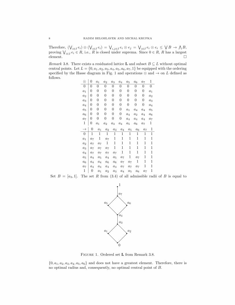
Remark 3.8. There exists a residuated lattice L and subset B ⊆ L without optimalcentral points. Let L = 0, a1, a2, a3, a4, a5, a6, a7, 1 be equipped with the orderingspecified by the Hasse diagram in Fig. 1 and operations ⊗ and → on L defined asfollows.

⊗ 0 a1 a2 a3 a4 a5 a6 a7 10 0 0 0 0 0 0 0 0 0a1 0 0 0 0 0 0 0 0 a1a2 0 0 0 0 0 0 0 0 a2a3 0 0 0 0 0 0 0 0 a3a4 0 0 0 0 0 0 0 0 a4a5 0 0 0 0 0 a1 a4 a4 a5a6 0 0 0 0 0 a4 a2 a4 a6a7 0 0 0 0 0 a4 a4 a4 a71 0 a1 a2 a3 a4 a5 a6 a7 1

→ 0 a1 a2 a3 a4 a5 a6 a7 10 1 1 1 1 1 1 1 1 1a1 a7 1 a7 1 1 1 1 1 1a2 a7 a7 1 1 1 1 1 1 1a3 a7 a7 a7 1 1 1 1 1 1a4 a7 a7 a7 a7 1 1 1 1 1a5 a4 a5 a4 a5 a7 1 a7 1 1a6 a4 a4 a6 a6 a7 a7 1 1 1a7 a4 a4 a4 a4 a7 a7 a7 1 11 0 a1 a2 a3 a4 a5 a6 a7 1

Set B = [a3, 1]. The set R from (3.4) of all admissible radii of B is equal to

1

a7

a5 a6

a4

a3

a1 a2

0

Figure 1. Ordered set L from Remark 3.8.

0, a1, a2, a3, a4, a5, a6 and does not have a greatest element. Therefore, there isno optimal radius and, consequently, no optimal central point of B.


Next we derive an explicit description of largest admissible radii and optimalcentral points for residuated lattices with square roots [5]: A complete residuatedlattice L has square roots if there is a function

√: L→ L satisfying

√a⊗√a = a,(3.5)

b⊗ b ≤ a implies b ≤√a,(3.6)

for every a, b ∈ L. As an example, the standard Lukasiewicz, product, and Godelalgebras on [0, 1] have sqaure roots. These are given by

√a =

a + 1

2for Lukasiewicz,

√a = ordinary number-theoretic square root

of a for product,√a = a for Godel.

Theorem 3.9. If L has square roots then every subset B ⊆ L has optimal centralpoints. For the corresponding largest admissible radius e of B it holds

(3.7) e =√∨

B →∧

B.

Proof. According to 1. of Lemma 3.4, (3.5), and (3.6), e is the largest admissibleradius of B. The rest follows from Theorem 3.1.

In general, the existence of optimal central points does not imply the existenceof square roots. As an example, for L = 0, 0.5, 1 equipped with Lukasiewiczoperations, every B ⊆ L has optimal central points. However, 0.5 does not have asquare root.

Theorem 3.10. L has square roots iff for every a ∈ L, [a, 1] has an optimal centralpoint such that for the corresponding admissible radius e we have e⊗ e = a.

Proof. If L has square roots, then according to Theorem 3.9, the largest admissibleradius of [a, 1] is e =

√1→ a =

√a and we have

√a⊗√a = a. Conversely, it follows

from the definitions and Theorem 3.1 that the admissible radius corresponding toan optimal central point of [a, 1] is the square root of a.

Corollary 3.11. If for every a ∈ L, [a, 1] has an optimal central point such thatfor the corresponding admissible radius e we have e⊗ e = a, then every B ⊆ L hasoptimal central points.

4. Optimal approximation algorithms

We now consider the following type of problems. Given a set M ⊆ L, find asmall set K ⊆ L which approximates M . The degree appr(M,K) to which M ⊆ Lis approximated by K ⊆ L is defined by

(4.1) appr(M,K) =∧

a∈M∨

b∈K(a↔ b).

appr(M,K) can be seen as a truth degree of “for every a ∈M there is b ∈ K suchthat a and b are similar”. Clearly, appr(M,K) = 1 for M ⊆ K, and K1 ⊆ K2

implies appr(M,K1) ≤ appr(M,K2). Consider the following problems.

Problem 1 Given a finite M ⊆ L and a threshold e ∈ L, find K ⊆ L such that


(1) K approximates M to degree at least e, i.e.,

(4.2) appr(M,K) ≥ e,

(2) there is no K ′ with |K ′| < |K| for which appr(M,K ′) ≥ e.

Problem 2 Given a finite M ⊆ L and a threshold e ∈ L, find K ⊆ L satisfying(1) and (2) of Problem 1, and

(3) For any K ′ with |K ′| = |K|,(4.3) appr(M,K) ≥ appr(M,K ′),

i.e., among the sets with |K| elements, K provides the best approximationof M .

In the rest of this section, we assume that the complete residuated lattice L islinearly ordered, i.e., a ≤ b or b ≤ a for every a, b ∈ L. The following theoremprovides a universal description of sets K satisfying (4.2).

Theorem 4.1. 1. Let Ω ⊆ 2L be a covering of M and ϕ : Ω→ L a mapping suchthat for any B ∈ Ω, ϕ(B) ∈ Ce(B). Then Ω consists of blocks of ≈e2 and K = ϕ(Ω)satisfies (4.2).

2. If a finite K ⊆ L satisfies (4.2) then Ω = Be(b) | b ∈ K ⊆ 2L is a setof blocks of ≈e2 that forms a covering of M . Moreover ϕ : Ω → L defined byϕ(Be(b)) = b satisfies ϕ(B) ∈ Ce(B).

Proof. 1. Since Ce(B) 6= ∅, the first assertion follows from Lemma 2.10. Since Ω is acovering of M , for every a ∈M there exists B ∈ Ω containing a. From the definitionof Ce(B), we get a↔ ϕ(B) ≥ e and from ϕ(B) ∈ K we get

∨b∈K a↔ b ≥ e proving

(4.2).2. Every B ∈ Ω is a closed ball with radius e, hence also a block of ≈e2 due

to Lemma 2.10. For a ∈ M let c ∈ K be such that a ↔ c =∨

b∈K a ↔ b (such cexists since K is finite and L is linearly ordered). (4.2) implies a ↔ c ≥ e, hencea ∈ Be(c) and Ω is a covering of M . ϕ(B) ∈ Ce(B) means c ∈ Ce(Be(c)) which istrue due to 1. of Lemma 2.9.

Example 4.2. Let L = [0, 1]2 with Lukasiewicz structure, M = L, e = 〈0.25, 0.25〉.Then

K = 〈0, 0〉, 〈0.5, 0〉, 〈1, 0〉, 〈0, 0.5〉, 〈0, 1〉satisfies (4.2) because appr(M,K) = 〈1, 1〉 ≥ e. However, Ω = Be(b) | b ∈ K isnot a covering of M because 〈1, 1〉 does not belong to any Be(b), b ∈ K. Hence, 2.from Theorem 4.1 does not hold for non-linear residuated lattices.

We now present two algorithms which provide solutions to Problem 1. The firstalgorithm constructs K going through L upwards.

Algorithm 4.3.

1: INPUT: M, e2: OUTPUT: K satisfying 1. and 2. of Problem 1

3: K ← ∅4: while M is not empty do

5: min ← min(M)6: add e→ min to K7: remove from M every element ≤ (e⊗ e)→ min


8: endwhile

9: return K

The second one constructs K going through L downwards.

Algorithm 4.4.

1: INPUT: M, e2: OUTPUT: K satisfying 1. and 2. of Problem 1

3: K ← ∅4: while M is not empty do

5: max ← max(M)6: add e⊗ max to K7: remove from M every element ≥ e⊗ e⊗ max

8: endwhile

9: return K

Lemma 4.5. 1. Let the set Ku produced by Algorithm 4.3 consist of elementsku1 < · · · < kup , let K ⊆ L, consisting of elements k1 < · · · < kq, approximate M todegree at least e. Then q ≥ p and for any i, 1 ≤ i ≤ p, kui ≥ ki.

2. Let the set Kl produced by Algorithm 4.4 consist of elements kl1 < · · · < klp,let K ⊂ L, consisting of elements k1 < · · · < kq, approximate M to degree at leaste. Then q ≥ p and for any i, 1 ≤ i ≤ p, kli ≤ ki.

Proof. 1. Let Ω = Be(b) | b ∈ K. By part 2 of Theorem 4.1, Ω is a covering ofM .

Suppose that the set of all i ≤ min(p, q) such that kui < ki is not empty anddenote its least element by j. Since ku1 = e→

∧M then ku1 is equal to the greatest

a ∈ L such that a↔∧M ≥ e (Theorem 2.4), which means that j > 1. Denote by

min the least element remaining in M after j − 1 steps. From min > kuj−1 ≥ kj−1and min /∈ Be(k

uj−1) we obtain min /∈ Be(kj−1). Since kuj is equal to the greatest

b ∈ L such that min↔ b ≥ e then also min /∈ Be(kj). Thus, Ω is not a covering ofM , which is a contradiction.

It remains to be shown that q ≥ p. Indeed, if q ≤ p− 1 then kq ≤ kup−1 <∨

M .Since

∨M /∈ B(kup−1) then also

∨M /∈ B(kq) and Ω is not a covering of M .

Part 2. can be proved similarly.

As the next two theorems show, the algorithms indeed produce solutions toProblem 1.

Theorem 4.6. Algorithms 4.3 and 4.4 are correct. They terminate after at mostO(|M |) steps.

Proof. Since (e ⊗ e) → min ≥ min, at least one element of M , namely min, isremoved from M in every step in Algorithm 4.3. For Algorithm 4.4, since e⊗ e⊗max ≤ max, max is removed from M in every step. As a result, the algorithmsterminate after at most O(|M |) steps.

For Algorithm 4.3: In every step, all elements a ∈M ∩B, where B = [min, (e⊗e) → min], are removed from M and, at the same time, e → min is added toK. By Theorem 2.4, e ⊗ e → min is the greatest among all a ∈ L for whichmin ↔ a ≥ e ⊗ e. Hence, B is a block of ≈e2 and by Lemma 2.10, Ce(B) is non-empty. Set ϕ(B) = e → min. By Theorem 2.2, ϕ(B) ∈ Ce(B). Thus, condition 1


of Problem 1 follows from part 1 of Theorem 4.1. Condition 2 follows directly fromLemma 4.5.

The proof for Algorithm 4.4 is similar.

Futhermore, the algorithms provide upper and lower bounds for every set Kwhich is a correct output for Problem 1.

Theorem 4.7. Let the sets Ku and Kl produced by Algorithm 4.3 and Algorithm4.4 consist of elements ku1 < · · · < kup and kl1 < · · · < klp, respectively. If Kconsisting of k1 < · · · < kp satisfies appr(M,K ′) ≥ e, then

kl1 ≤ k1 ≤ ku1 , . . . , klp ≤ kp ≤ kup .

Proof. Follows directly from Lemma 4.5.

The following example shows that not every K = k1, . . . , kp for which kli ≤ki ≤ kui satisfies appr(M,K) ≥ e.

Example 4.8. Consider the standard Lukasiewicz algebra on L = [0, 1], M =0.5, 0.7, 0.8, and e = 0.9. Then Kl = 0.4, 0.7 and Ku = 0.6, 0.9. LetK = 0.4, 0.9. Then appr(M,K) = 0.8 < e.

Although the set K produced by Algorithm 4.3 or Algorithm 4.4 is optimal inthat it is one of the smallest sets for which appr(M,K) ≥ e, there can be a set K ′

of the same size, i.e., |K ′| = |K|, for which appr(M,K ′) > appr(M,K), i.e., K ′

provides a better approximation of M than K. From this point of view, the outputset K from Algorithm 4.3 and Algorithm 4.4 can be improved. Namely, it is easilyseen from the description of Algorithm 4.3 and Algorithm 4.4 that the set

Be(k) ∩M | k ∈ Kforms a partition of M . In general, k is not an optimal central point of Be(k)∩M .Therefore, we can improve K by replacing every k ∈ K by an optimal central pointof Be(k) ∩M .

By Theorem 3.9, if L has square roots, then any element from[√∧(Be(k) ∩M)⊗

∨(Be(k) ∩M),√∧

(Be(k) ∩M)→∧

(Be(k) ∩M)]

can be used to replace k. For instance, for M = 0.5, 0.7, 0.8 and K = Kl =0.4, 0.7 from Example 4.8, B0.9(0.7) ∩ M = 0.7, 0.8 and B0.9(0.4) ∩ M =0.5. Hence, 0.4 can be replaced by 0.5 (optimal central point of 0.5) and0.7 can be replaced by 0.75 (optimal central point of 0.7, 0.8). As a result,we get a set opt(Kl) = 0.5, 0.75 for which appr(M, opt(Kl)) = 0.95 > 0.9 =appr(M,K). In addition, we have Ku = 0.6, 0.9, opt(Ku) = 0.6, 0.8, but thistime appr(M, opt(Ku)) = 0.9 = appr(M,K).

As the next example shows, such improvement does not, in general, satisfy con-dition 3. of Problem 2. That is, replacement of points k in K by better points k′

which cover the same part of M , i.e., for which Be(k)∩M = Be(k′)∩M , does not

result in the best approximating set with size |K|.

Example 4.9. Consider the standard Lukasiewicz algebra on L = [0, 1], M =0, 0.1, 0.3, 0.7, 0.9, 1, and e = 0.9. Then Kl = 0, 0.2, 0.6, 0.9 and Ku = 0.1, 0.4,0.8, 1, opt(Kl) = 0, 0.2, 0.7, 0.95, opt(Ku) = 0.05, 0.3, 0.8, 1, appr(M,Kl) =


0.9, appr(M,Ku) = 0.9, appr(M, opt(Kl)) = 0.9, appr(M, opt(Ku)) = 0.9. How-ever, K = 0.05, 0.3, 0.7, 0.95 is a solution to Problem 2 for which appr(M,K) =0.95.

In what follows, we present an algorithm that provides a solution to Problem 2provided the largest admissible radii of subsets of L exist and may be determined.Due to Theorem 3.9, an important class of residuated lattices that satisfies thisassumption consists of residuated lattices with square roots.

Let thus M = m1 ≤ · · · ≤ mn and denote by r(A) the largest admissibleradius of A ⊆ L.

Algorithm 4.10.

1: INPUT: M, e2: OUTPUT: K solving Problem 2

3: K ′ ← output of Algorithm 4.3 for M, e4: q ← |K ′|5: e′ ← e6: repeat

7: K ← K ′

8: for i = 1 to n− 1 do

9: r′ ← minr([mi,m]) |m ∈M, r([mi,m]) > e10: if e′ < r′ then e′ ← r′

11: endfor

12: e ← e′

13: K ′ ← output of Algorithm 4.3 for M, e14: until |K ′| > q15: return K

Theorem 4.11. Algorithm 4.10 is correct. It terminates after at most O(|M |4)steps.

Proof. The algorithm starts by computing a set K ′ with q elements that approxi-mates M to degree at least e. The aim of loop 6–14 is to compute another set of qelements that approximates M to a largest possible degree d, larger than originale. To this end, the loop in 8–11 determines the least candidate e′ for such d. Thisis easily seen by realizing that r([mi,m]) is the radius of [mi,m] for any optimalcentral point of [mi,m], see Theorem 3.1. Any such optimal central point covers[mi,m]) and is a potential element of a new set of q elements that approximatesM to a higher degree than the lastly computed K ′. For e′, Algorithm 4.3 in line13 computes a new set K ′ that approximates M to degree at least e′. Due toLemma 4.5, this set has more than q elements if and only if no set with q elementsapproximates M to degree e′ (or larger). In this case, the candidate e′ may not beused a lower approximation of d and the loop 6–14 terminates. In the other case,e′ is taken as a lower approximation of d and the loop 6–14 is entered again toproduce and test another, larger candidate, until such a candidate exists. The lastcomputed set K ′ with q elements is therefore the output to Problem 2.

Within loop 8–11, r([mi,m]) is evaluated at most |M |·(|M |−1)2 = O(|M |2) times.

Loop 8–11 is run within loop 6–14 which itself is run at most |M |·(|M |−1)2 = O(|M |2)

times, yielding the total of O(|M |4) steps in the worst case.


Note that after Algorithm 4.10 finishes, we may run Algorithm 4.4 on M and e′

where e′ is the value in Algorithm 4.10 for which the output of Algorithm 4.10 wascomputed. According to Theorem 4.7, the outputs produced by Algorithm 4.10and Algorithm 4.4 provide us with lower and upper bounds for every solution toProblem 2.

Acknowledgement Supported by project No. CZ.1.07/2.3.00/20.0059. Theproblem and the first results were presented at the IPMU’08 conference.

References

1. N. Galatos, P. Jipsen, T. Kowalski, H. Ono, Residuated Lattices: An Algebraic Glimpse at

Substructural Logics, Elsevier, 2007.

2. J. A. Goguen, The logic of inexact concepts, Synthese 19(1968–69), 325–373.3. S. Gottwald, A Treatise on Many-Valued Logic, Research Studies Press, England, 2001.

4. P. Hajek P, Metamathematics of Fuzzy Logic, Kluwer, Dordrecht, 1998.

5. U. Hohle, Commutative, residuated l-monoids, In: Non-classical logics and their applicationsto fuzzy subsets, Kluwer, Dordrecht, 1995, pp. 53–106.

6. M. F. Janowitz, Residuation Theory, Elsevier, 1970.

7. E. P. Klement, R. Mesiar, E. Pap, Triangular Norms, Kluwer, Dordrecht, 2000.8. M. Ward, R. P. Dilworth, Residuated lattices, Trans. Amer. Math. Soc. 45(1939), 335–354.

9. R. Wille, Complete tolerance relations of concept lattices, Contributions to General Algebra,

vol. 3, Holder-Pichler-Tempsky, Wien, 1985, pp. 397–415.

Palacky University, Olomouc, Czech Republic

E-mail address: [email protected]

Palacky University, Olomouc, Czech RepublicE-mail address: [email protected]

CENTRAL POINTS AND APPROXIMATION IN RESIDUATED LATTICES

Documents

Transcript of CENTRAL POINTS AND APPROXIMATION IN RESIDUATED LATTICES