
CENTRAL BANK LIQUIDITY MANAGEMENT: THEORY AND · PDF fileCENTRAL BANK LIQUIDITY MANAGEMENT:...
38
1 CENTRAL BANK LIQUIDITY MANAGEMENT: THEORY AND EURO AREA PRACTICE Ulrich Bindseil * APRIL 2000 Abstract The “liquidity management” of a central bank is defined as the framework, set of instruments and especially the rules the central bank follows in steering the amount of bank reserves in order to control their price (i.e. short term interest rates) consistently with its ultimate goals (e.g. price stability). The note presents a basic theory of liquidity management in a framework of substantial reserve requirements and averaging, focusing on the relationship between quantities (central bank balance sheet items) and overnight rates and the involved signal extraction problems. Some elements of a “normative” theory of liquidity management are suggested. The note then turns to liquidity management in practice in the case of the Eurosystem, describing the experience of the first 15 months. A simple regression analysis, explaining the evolution of EONIA rates by the liquidity situation, illustrates the empirical relevance of the exposed theoretical relationships. JEL classification: D 84, E52 Keywords: Monetary policy instruments, central bank liquidity management, money market, signal extraction. * European Central Bank, DG Operations, Kaiserstrasse 29, 60311 Frankfurt am Main, Germany. E-mail: [email protected]. Comments from Denis Blenck, Francesco Papadia, and Franz Seitz helped to improve the paper. The views expressed are those of the author and not necessarily those of the ECB.
Transcript of CENTRAL BANK LIQUIDITY MANAGEMENT: THEORY AND · PDF fileCENTRAL BANK LIQUIDITY MANAGEMENT:...

1
CENTRAL BANK LIQUIDITY MANAGEMENT:
THEORY AND EURO AREA PRACTICE
Ulrich Bindseil*
APRIL 2000
Abstract
The “liquidity management” of a central bank is defined as the framework, set of instruments and
especially the rules the central bank follows in steering the amount of bank reserves in order to control
their price (i.e. short term interest rates) consistently with its ultimate goals (e.g. price stability). The
note presents a basic theory of liquidity management in a framework of substantial reserve
requirements and averaging, focusing on the relationship between quantities (central bank balance
sheet items) and overnight rates and the involved signal extraction problems. Some elements of a
“normative” theory of liquidity management are suggested. The note then turns to liquidity
management in practice in the case of the Eurosystem, describing the experience of the first 15
months. A simple regression analysis, explaining the evolution of EONIA rates by the liquidity
situation, illustrates the empirical relevance of the exposed theoretical relationships.
JEL classification: D 84, E52
Keywords: Monetary policy instruments, central bank liquidity management, money market,signal extraction.
* European Central Bank, DG Operations, Kaiserstrasse 29, 60311 Frankfurt am Main, Germany. E-mail:
[email protected]. Comments from Denis Blenck, Francesco Papadia, and Franz Seitz helped to improve the paper. The
views expressed are those of the author and not necessarily those of the ECB.
2
1. INTRODUCTION
The “liquidity management” of a central bank is defined here as the framework, set of instruments and
rules the central bank uses in steering the amount of bank reserves in order to control their price (i.e.
short term interest rates) consistently with its ultimate goals (e.g. price stability). The central bank’s
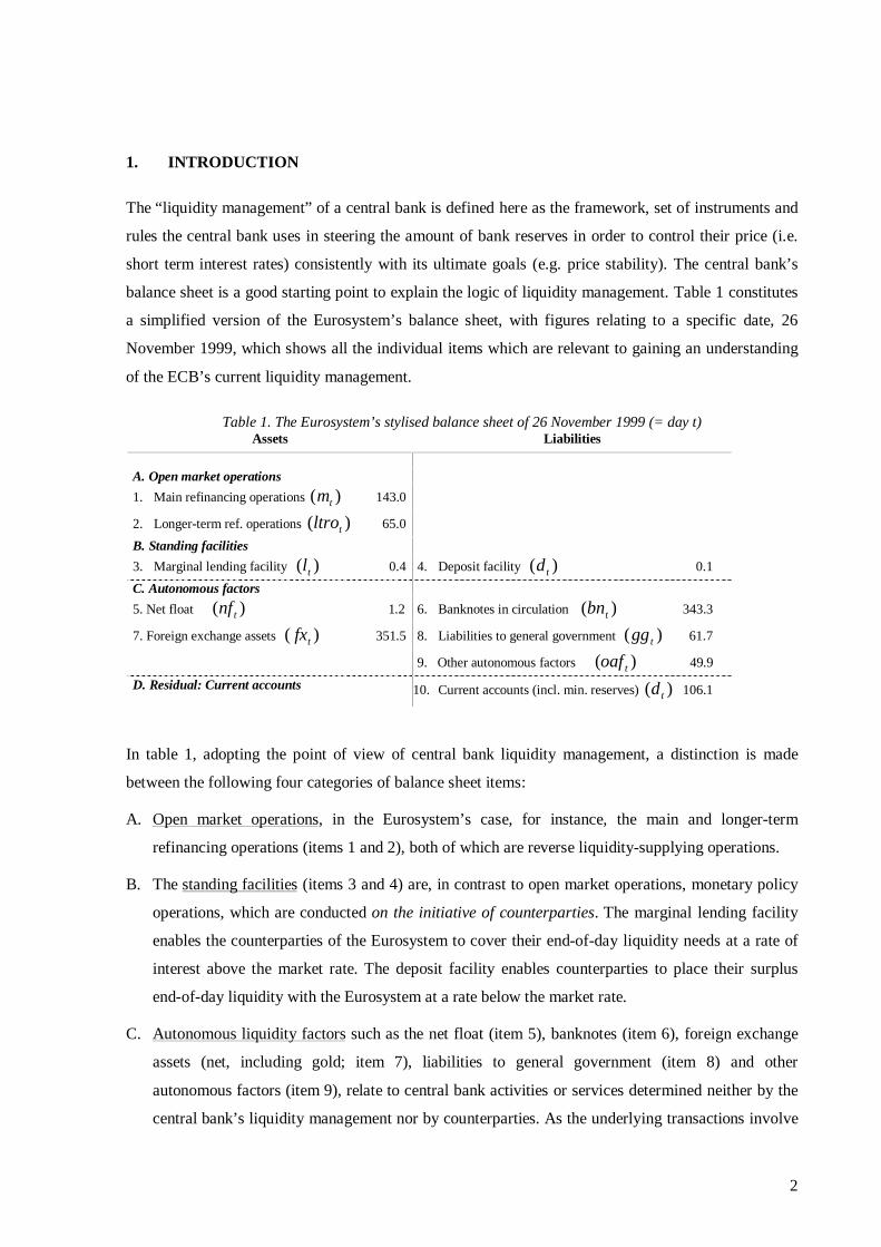
balance sheet is a good starting point to explain the logic of liquidity management. Table 1 constitutes
a simplified version of the Eurosystem’s balance sheet, with figures relating to a specific date, 26
November 1999, which shows all the individual items which are relevant to gaining an understanding
of the ECB’s current liquidity management.
Table 1. The Eurosystem’s stylised balance sheet of 26 November 1999 (= day t)Assets Liabilities
A. Open market operations
1. Main refinancing operations )( tm 143.0
2. Longer-term ref. operations )( tltro 65.0
B. Standing facilities
3. Marginal lending facility )( tl 0.4 4. Deposit facility )( td 0.1
C. Autonomous factors
5. Net float )( tnf 1.2 6. Banknotes in circulation )( tbn 343.3
7. Foreign exchange assets )( tfx 351.5 8. Liabilities to general government )( tgg 61.7
9. Other autonomous factors )( toaf 49.9
D. Residual: Current accounts 10. Current accounts (incl. min. reserves) )( td 106.1
In table 1, adopting the point of view of central bank liquidity management, a distinction is made
between the following four categories of balance sheet items:
A. Open market operations, in the Eurosystem’s case, for instance, the main and longer-term
refinancing operations (items 1 and 2), both of which are reverse liquidity-supplying operations.
B. The standing facilities (items 3 and 4) are, in contrast to open market operations, monetary policy
operations, which are conducted on the initiative of counterparties. The marginal lending facility
enables the counterparties of the Eurosystem to cover their end-of-day liquidity needs at a rate of
interest above the market rate. The deposit facility enables counterparties to place their surplus
end-of-day liquidity with the Eurosystem at a rate below the market rate.
C. Autonomous liquidity factors such as the net float (item 5), banknotes (item 6), foreign exchange
assets (net, including gold; item 7), liabilities to general government (item 8) and other
autonomous factors (item 9), relate to central bank activities or services determined neither by the
central bank’s liquidity management nor by counterparties. As the underlying transactions involve

3
the same means of payment, namely central bank money, transactions affecting these items have
exactly the same liquidity-providing or liquidity-absorbing effect as monetary policy-related
transactions.
D. The current account holdings (or “reserves” or “deposits”) of counterparties with the Eurosystem
(item 10) is considered from the point of view of liquidity management as a residual position
which balances the balance sheet. All operations of the Eurosystem ultimately affect the banks’
current accounts (as long as they do not net out). By transforming the balance sheet identity,
current accounts can always be determined from the following equation:
)()( tttttttttt fxnfoafgglbndlltromc −−++−−++= (1)
= open market operations + use of standing facilities - autonomous factors
One may also interpret this equation as the supply function of current account holdings (“reserves”) of
counterparties with the central bank. To complete the basics of a model of the market for banks’
reserves with the central bank, the demand side has to be added. In the case of the Eurosystem, reserve
requirements, denoted by v, to be fulfilled on average in the maintenance period, constitute the
essential demand component of reserves. Since not fulfilling reserve requirements implies
considerable penalties, and since shortages can always be covered through recourse to marginal
lending on the last day of the maintenance period, reserve requirements will always be fulfilled by
counterparties, except for management errors. Beyond reserve requirements, banks also have some
demand for excess reserves, named x (defined as daily average over the maintenance period). In the
case of the Eurosystem, around 0.7% of total current accounts correspond to excess reserves. In the
case of central banks without reserve requirements, excess reserves by definition amount to 100% of
current account deposits.
Denoting by 1…T the T days of the reserve maintenance period and by capitals the sums over the
maintenance period of the different items (e.g. ∑=
=T
ttcC
1
), the market for current account holdings
with the central bank in a specific reserve maintenance period can be described by the following
market equation:
XVFXNFOAFGGLBNDLLTROM
CC ds
+=−−++−−++⇔
=
)()( (2)

4
As will be described in more detail in section 2, the only interest rate elastic components in this
equation are the recourses to the standing facilities, which will hence play the crucial role in achieving
the market equilibrium.1
The logic of a central bank’s liquidity management in terms of the described four types of balance
sheet items can be summarised roughly as follows: The central bank attempts to provide liquidity
through its open market operations in a way that, after taking into account the effects of autonomous
liquidity factors, counterparties can fulfil their reserve requirements on average over the reserve
maintenance period without systematic recourse to the standing facilities. If the ECB provides more
(less) liquidity than this benchmark, counterparties will use on aggregate the deposit (marginal
lending) facility.
This note proceeds as follows. Section 2 will present a basic theory of liquidity management in the
described framework, focusing on the relationship between quantities (central bank balance sheet
items) and overnight rates and the involved signal extraction problems. Some considerations with
regard to elements of a “normative” theory of liquidity management close this section. Section 3 then
turns to liquidity management in practice in the case of the Eurosystem, describing the experience of
the first 15 months and providing a description and first assessment of the chosen liquidity
management strategy. Section 4 concludes the paper.
2. ELEMENTS OF A THEORY OF LIQUIDITY MANAGEMENT
2.1 Introduction
The aim of this section is to provide some elements of a theory of central bank liquidity management.
The theory of central bank liquidity management has to be clearly distinguished from the macro-
economic literature starting with the seminal paper by Poole [1970] (for a recent survey see Walsh
[1998], Chapter 9). Central bank liquidity management, at least as understood here, refers to the
shortest end of implementation of monetary policy, and assumes that the only channel of
“communication” between the macro-economy and liquidity management is the operational target rate
of the central bank (e.g. the overnight rate target). It is furthermore assumed that in the very short run
under consideration, macro-economic shocks never affect directly the equilibrium value of the
variable, which is considered as the operational target, but only through an implied change of the
target value of this variable decided by the central bank. Even though the literature following Poole
[1970] often makes use of a terminology such as „operating procedures“ and „the instrument-choice“
problem, it in fact focuses more on the shorter-term macro-economic strategy of the central bank than
1 Note that the market equilibrium condition (2) can easily be re-arranged to represent a market equilibrium for base money,namely by shifting banknotes (BN) to the right hand side of the equation and interpreting it as one component of the demand

5
on the actual day-to-day implementation of monetary policy, and does not really deal with what
central bankers normally understand under these terms.
Liquidity management takes place within an operational framework, and the choice of the operational
framework is itself preceded by the existence of some environment. A theory of liquidity management
has clearly to distinguish between these different categories. While the theory outlined in this section
focuses on liquidity management, it is worth briefly listing the main elements of the operational
framework and the environment and to provide the assumptions that are made with their regard.
Mainly three elements of the environment affecting the optimal choice of the operational framework
and the liquidity management strategy have to be distinguished:
(a) the institutional features of the inter-bank money market. The relationship between the
relevant quantities (liquidity) and prices (overnight inter-bank rates) is not totally independent
from the structure and efficiency of the inter-bank money market. We assume a high degree of
efficiency of the inter-bank market, such that problems relating to the distribution of funds within
the banking sector can be ignored. This assumption is largely justified in the case of the euro area.
(b) the time series properties and forecastability of the autonomous liquidity factors. It is
assumed that autonomous factors are subject to a relevant volatility and ex ante uncertainty. With
regard to forecasting, it is assumed that changes in the autonomous factors can be forecast to some
extent by the central bank and by counterparties, but that both players cannot forecast them
perfectly and that the central banks’ forecasts are better than those of counterparties. Both
assumptions are adequate for all major central banks.
(c) The time series properties of the operational target, e.g. of the average short-term overnight
rate target of the central bank. The central bank can change the target value of its operational
target variable at any meeting of the relevant Governing body due to new insights on which short-
term rates are compatible in the prevailing macro-economic environment, with the ultimate goals
of the central bank. It is assumed that changes of the operational target of the central bank cannot
be anticipated perfectly by money market players, i.e. there is potential asymmetry between the
central bank’s and the market’s knowledge on the operational target. Again, these assumptions are
in line with the reality of major central banks.
Finally, two main elements of the operational framework, which can be specified by the central bank
on the basis of normative considerations, should be distinguished.
(d) The menu of monetary policy instruments. It is assumed that the central bank has at its disposal
a wide range of open market operations, both for the provision and absorption of liquidity and that
for base money.

6
counterparties have sufficient collateral to cover liquidity providing operations of the central bank.
With regard to the standing facilities, at least the existence of a marginal lending facility with
overnight maturity is assumed. A deposit facility is also assumed, however noting that the case of
a central bank without a deposit facility is not really different, since it can be interpreted as having
a deposit facility with a zero remuneration. These assumptions are again adequate for all major
central banks.
(e) The reserve requirement system. It is assumed that the central bank imposes reserve
requirements, the fulfilment of which has to be achieved only on average within a reserve
maintenance period of e.g. one month, and that the reserve requirements are sufficiently high to
provide buffers against the largest aggregate autonomous factor fluctuations. These assumptions
are adequate for the Eurosystem, but to a lesser extent for the Federal Reserve System and the
Bank of Japan with their relative low reserve requirements (relative in comparison to the reserve
requirements of the Eurosystem and relative to the respective volatility of their autonomous
factors). The assumptions may be even less adequate for the Bank of England, which does not
impose any reserve requirements subject to averaging. In the case of these latter central banks,
liquidity management has to focus to a much higher degree on daily developments and hence to
operate on the basis of daily, or more than daily, open market operations. Nevertheless, many of
the problems of liquidity management discussed in the following can also be applied to such an
environment.
2.1 The general relationship between liquidity and overnight rates
Supply and demand for deposits of banks with the Eurosystem determine their price, the overnight
rate. As seen above, the supply of reserves is given by the net effect of the liquidity provided through
monetary policy operations and by autonomous factors. The demand for reserves comes from the
banks’ need to fulfil reserve requirements through the holding of reserves and some further small
demand for “excess” reserves, arguably connected to payment needs. The price for reserves is a short-
term inter-bank rate, generally the overnight maturity plays a key role in terms of volume and is often
the focus of attention since it has the shortest relevant maturity and is therefore the origin of the entire
yield curve.
Like many other markets, the market for reserves is interesting owing to its uncertainty. In a system
of minimum reserve requirements which, on average, have only to be fulfilled in a maintenance period
of one month, such as that of the Eurosystem, banks face an inter-temporal optimisation problem when
minimising the cost of holding required reserves over the maintenance period. The opportunity cost of
holding reserves on one day is the inter-bank overnight rate on that day. Banks will thus have an

7
incentive to hold reserve surpluses (or accumulate reserve deficits) whenever the market rate is low
(high) in relation to future expected overnight rates within the maintenance period. This behaviour on
the part of banks will tend to stabilise market rates as, in order for the daily market to clear, overnight
rates will tend to be aligned with future expected overnight rates within the maintenance period.
Overnight rates will, thus, be determined not only by current or past conditions, but also by
expectations with regard to expected liquidity conditions in the remainder of the reserve maintenance
period.
We shall now assume for a moment that there is no uncertainty concerning either autonomous factors
or the liquidity supply through monetary policy operations in the remainder of the reserve maintenance
period. In this setting, reserves are obviously either short or long in relation to reserve requirements, in
which case the marginal utility of funds obtained in the inter-bank market, and therefore their price,
either rises to the marginal lending rate, or drops to the deposit rate. In the entire maintenance period,
the overnight rate would therefore correspond, under the assumption of perfect foresight with regard to
liquidity conditions, to one of the standing facility rates relevant at the end of the maintenance period.
In terms of the balance sheet items introduced in the previous section, this may be expressed as
follows. Denote by tttttt ltrooafnfggbna −−−+= the sum of all autonomous factors minus the
longer term refinancing operation (which can be treated as an autonomous factor in the case of the
Eurosystem) and by A the corresponding sum over the maintenance period. Then, one may call M-A
the amount of “non-borrowed” reserves, to use a term applied usually in the US. Furthermore, denote
by di the rate of the deposit facility and by mli the rate of the marginal lending facility, with mld ii < .
The only interest rate elastic elements of the market equilibrium condition for bank deposits with the
central bank, the standing facilities, have the following functional form:
MAiLii
iLii
iLii
ml
ml
ml
−==
∞=>∀
=<∀
)(:
)(:
0)(:
:
AMiDii
iDii
iDii
d
d
d
−==
∞=<∀
=>∀
)(:
)(:
0)(:
: (3)
The overnight interest rate that clears the market for central bank deposits is then determined by:
XVOAFNFGGLBNiDiLLTROM +=−−+−−++ )())()(( (4)
The market is represented graphically in chart 1 for the case of a recourse to the marginal lending
facility.
- insert chart 1 here -

8
Now we shall consider the more interesting case in which the liquidity supply and the rates of the
standing facilities are uncertain in the sense that the banking sector has a collective subjective density
function for the relevant liquidity factors in its mind. Denote now with ti the overnight rate on day t.
The basic relationship between quantities and prices (overnight rates) under the assumptions made
above (especially the one of perfect inter-bank markets and large reserve requirements) is then
described by the following equation:
))()()(())()()((
)"(")()"(")()(...)( 1
∫∫∞
∞−
+
−−+−−=
+====
V
btd
bt
Vb
tmlbt
dbtml
btT
btt
btt
AMdAMfiEAMdAMfiE
longPiEshortPiEiEiEi
(5)
In words: the overnight rates on any day will correspond to the weighted expected rates of the two
standing facilities, the weights being the respective probabilities that the market will be short or long
at the end of the maintenance period before having recourse to standing facilities. Ex ante, rates are
constant within the maintenance period, i.e. the expected overnight rates for the remainder of the
maintenance period are all identical. Ex post, rates do not have to be constant since news about the
expected end of maintenance period standing facilities rates and the net liquidity supply may occur at
any moment in time.
Obviously, expectations, i.e. the subjective density functions the banking sector assigns to the non-
borrowed reserves, M-A, and the expectations with regard to standing facility rates, are the major
challenge for a calibration of this equation. Neither expectations with regard to standing facility rates,
nor expectations with regard to autonomous factors, nor expectations concerning open market
operations can be measured directly.
2.2 The basic signal extraction problem
In the previous subsection, it was argued that the supply side of the market for deposits is subject to
two uncertainties: the one associated to the available quantity of non-borrowed reserves and the one
associated to the prices at which surpluses or deficits of reserves will be neutralised, i.e. to the rates of
the standing facilities. In terms of the supply schedule of deposits, the first uncertainty is the one
regarding the location of the vertical part of the supply curve (i.e. the value of M-A), while the second
concerns the points where the vertical part of the supply curve kinks into the horizontal parts due to
the standing facilities (i.e. the values of mld ii , ).

9
It has been assumed that the central bank has superior information with regard to all relevant uncertain
supply parameters: it has better forecasts of autonomous factors; it controls its open market operations;
it knows more about its intentions with regard to the rates of the standing facilities. However, the
actions of the central bank may reveal part of its superior information. This creates a signal extraction
problem for counterparties: by observing the actions of the central bank (e.g. its allotment decisions in
open market operations, statements of members of the Governing bodies with regard to intentions to
change central bank rates, etc.), the banks will be able to extract some part of its superior information.
However, this information will be noisy as long as, assuming a linear relationship between observed
and unobserved variables, the number of observed variables is lower than the number of unobserved
ones. To allow a very basic representation of the core signal extraction problem on the money market,
take the following simplifying assumptions:
� The maintenance period consists of exactly one day. On this day, the sequence of events is as
follows: first, the central bank conducts its open market operations, the allotment amount being
immediately published. Second, the inter-bank market takes place and the overnight rate is fixed
that clears the market. Third, the realisation of autonomous factors takes place. Finally, the banks
take recourse to standing facilities.
� Autonomous factors are white noise, i.e. ηε +=a , with ηε , being identically and independently
distributed random variables with variance 22 , ηε σσ (the index for the day of the maintenance
period, t, is dropped). The central bank is assumed to have perfect forecasts of ε , but it has no
prior information on η . Banks are assumed to have no prior information on any of the two
variables.
� The rate of the deposit facility, di , is set to zero for the sake of simplicity. The rate of the marginal
lending facility, mli , is positive, but also not subject to uncertainty.
� In deciding on the allotment volume in its open market operation, the central bank takes into
account its autonomous factor forecasts and to where, in the corridor set by standing facilities, it
wants to steer the overnight rate. To simplify calculations, it is assumed that the central bank has
no operational target in the form of the overnight rate, but in the form of liquidity surplus or deficit
at the end of the maintenance period, denoted γ . The higher the target liquidity deficit, the higher
will be the likelihood of a recourse to the marginal lending facility, and the closer the overnight
rate will be to the rate of this facility, at least to the extent anticipated by counterparties. As the
central bank observes permanently news on the state of the macro-economy and on dangers to
SULFH�VWDELOLW\��WKH�WDUJHWHG� �PD\�FKDQJH��$VVXPH�WKDW�WKH�LQQRYDWLRQV� µ �WR� �DUH�ZKLWH�QRLVH��L�H�
that µγγ += −1 , with µ being an identically and independently distributed random variable with
an expected value of zero variance 2µσ .

10
� Excess reserves are zero, i.e. the entire demand for reserves is given by reserve requirements.
The signal extraction problem of banks in this minimalist setting can be described as follows: When
observing the allotment decision of the central bank, banks are aware that the allotment amount
reflects two unobserved stochastic variables that are linked through a linear relationship to the
observed amount. Knowing the two unobserved variables separately would be, however of crucial
interest for counterparties since this would allow to know more about the marginal value of reserves at
the end of the maintenance period, and therefore about their “fair” price in the inter-bank market
session. For instance, an ample allotment decision may simply reflect the fact that the central bank has
D� KLJK� DXWRQRPRXV� IDFWRU� IRUHFDVW� RI� �� WKH� LQQRYDWLRQ� LQ� � KDYLQJ� EHHQ� QHJOLJLEOH�� 7KHQ�� WKH� IDLU
overnight rate would remain at its previous levels, reflecting the unchanged likelihood of recourse to
WKH�PDUJLQDO� OHQGLQJ�IDFLOLW\�� ,I�KRZHYHU� LW�KDV�QR� LQIRUPDWLRQ�RQ�DXWRQRPRXV� IDFWRU� IORZV�� L�H�� � LV
close to zero, then the ample allotment decision would indicate a change of monetary policy
intentions, and the fair overnight rate would move downwards. Formally, this simple signal extraction
problem can be described as follows. Counterparties observe the allotment amount m and know the
linear structure:
γε −+= vm (6)
Applying the standard signal extraction formula (see for instance Sargent [1979]), one obtains the
following estimators for the unobserved variables (the “b” in the superscript indicates that those are
the expectations formed by banks):
)()(),()( 22
2
22
2
vmEvmE bb −+
=−+
=εγ
ε
εγ
γ
σσσε
σσσ
γ (7)
The variances of the errors of the estimates will be:
22
422
22
422 ))((,))((
εγ
εε
εγ
γγ σσ
σσεεσσ
σσγγ
+−=−
+−=− bb EEEE (8)
The overnight rate in the inter-bank market will amount to:
))()(( ∫−
∞−
++=vm
bm dfii ηεηε (9)
The subjective density function )( ηε +bf has an expected value of )(22
2
vm −+ εγ
ε
σσσ
and a variance
of 22
422
εγ
εεη σσ
σσσ+
−+ .

11
Consider now an example with )1,10,10(),,( 222 =µεη σσσ , v = 100, %5=mi and 01 =−γ . If
counterparties observe an allotment amount m=99, they will estimate the central banks target with
UHJDUG� WR� WKH� HQG� RI� PDLQWHQDQFH� SHULRG� OLTXLGLW\� VXUSOXV�� �� WR� ±����� DQG� WKH� DXWRQRPRXV� IDFWRU
forecast of the central bank to –10/11. The residual variance of the counterparties’ autonomous factor
forecast would be 10+10-100/11 = 10.91. Assuming normally distributed shocks, the overnight rate
would therefore be equal to %44.2)0275.0(05.0)91.10/)11/101(()1( =−=+−=−= GGiFii mm ,
where G() is the Gauss (standardised normal) cumulative distribution. Chart 2 indicates the
relationship between the allotment volume and the overnight rate under the chosen parameters..
- Insert Chart 2 -
Since the signal extraction is noisy, the interest rate will in fact not correspond, day after day, to the
LQWHUHVW� UDWH� FRPSDWLEOH� ZLWK� �� L�H�� LQWHUHVW� UDWHV�ZLOO� EH� QRLV\� DURXQG� WDUJHW� UDWHV�� WKH� QRLVH� EHLQJ
implied by the noise in the autonomous factors. Note that under the assumed random walk of the
targeted end of maintenance period liquidity surplus, the volatility of short term rates will be fully
transmitted along the yield curve and would therefore also affect the rates deemed relevant for the
transmission of monetary policy2. There are four potential ways out of this signal extraction problem,
all of which consist in making the signal extraction trivial:
� The central bank may publish its autonomous factor forecast� ��7KHQ��WKH�REVHUYDWLRQ�RI�m can
EH� PDSSHG� ZLWKRXW� QRLVH� LQWR� �� WKH� WDUJHW� RI� WKH� FHQWUDO� EDQN� ZLWK� UHJDUG� WR� WKH� HQG� RI
maintenance liquidity deficit, and into an adequate overnight rate.
� The central bank may ignore its autonomous factor forecasts, i.e. it may simplify its allotment
UXOH�WR�P� �Y��� ��7KHQ��DJDLQ��WKH�OLQHDU�UHODWLRQVKLS�ZRXOG�PDS�RQO\� RQH�XQREVHUYHG� LQWR� RQH
observed variable, and extracting the unobserved one would again be trivial. However, this
strategy would come at the price of a higher variance of the recourse to the standing facilities,
since the central bank would not neutralise any longer the anticipated autonomous factor shocks.
� The central bank may announce its target�HQG�RI�PDLQWHQDQFH�OLTXLGLW\�GHILFLW� , or alternatively,
the inter-bank rate compatible with this expected liquidity deficit at the end of the maintenance
period. This solution was adopted for instance by the Federal Reserve System in 1995.3 Fixed rate
2 Assuming the rational expectations hypothesis of the term structure of interest rates.3 The communication approach chosen by the Federal Reserve System is explained for instance in Federal Reserve Bank ofNew York [2000]. The decision making for US monetary policy takes place in the Federal Open Market Committee (FOMC)which meets 8 times a year. If there is a change in the stance of monetary policy by the FOMC, it is announced to the publicshortly after the meeting, on the same day. The announcement gives the new intended average level of the federal funds rate,along with a brief rationale for the change in policy stance. “The currently applied disclosure procedure was inauguratedonly in 1995. Before, the FOMC’s policy decisions were announced with a five-to-eight week lag, through the release of itsminutes, which contain the domestic policy directive”. However, market participants “closely watched the Desk’s operationsto detect policy signals. The use of open market operations to signal policy changes created, at times, considerablecomplications for the Desk, especially when the funds rate and the reserve estimate gave conflicting signals. Just as

12
tenders (as employed so far by the Eurosystem in its main refinancing operations) may also be
viewed as an implicit announcement of the target average overnight rate.
� Finally, the central bank may stick to a strategy to always target the mid of the corridor, i.e. to
DOZD\V�VHW� ���RU�DW� OHDVW�WR�QHYHU�FKDQJH� LWV�SROLF\�WRZDUGV� ��6LQFH� LW� LV�SRVVLEOH�WR�DGMXVW�WKH
rates of the standing facilities at any degree of precision, one may argue that it is never required
for monetary policy reasons to fine-tune the position of short term rates within the corridor
through a specific liquidity policy.
2.3 Towards a normative theory of central bank liquidity management
The liquidity management strategy of the central bank and the operational framework are the two main
elements of the day to day implementation of monetary policy. While almost all elements of the
operational frameworks of central banks are generally public, the liquidity management strategy is
normally something that has to be inferred by observers from the actual behaviour of the central bank.
The concept of a liquidity management “strategy” of the central bank does not imply a total pre-
commitment of the central bank, i.e. to opt totally for “rules” instead of for “discretion” in the
implementation of monetary policy. It reflects the idea that there are some systematic elements in each
liquidity management approach and that if all these systematic components that relate the liquidity
management decisions of the central bank to specific “information” variables are defined as the
strategy, the residual components of the actual liquidity management behaviour should be non-
correlated (orthogonal) to those information variables. Therefore, in the equation specifying the
mapping of information variables into the liquidity management strategy, the other components can be
treated as orthogonal white noise. The liquidity management strategy of a central bank consists of
several interrelated sub-elements, namely:
(1) the liquidity provision through open market operations;
(2) the choice of instruments and procedures in the different open market operations (e.g. outright
versus reverse operations, fixed versus variable rate tenders, etc.);
(3) further elements of the information policy (e.g. publishing or not autonomous factor forecasts).
What aims should the central bank follow when specifying, also as a function of all relevant
environmental parameters, its implementation of monetary policy, i.e. its operational framework and
importantly, the Desk also faced considerable risks that day-to-day technical or defensive operations would be viewed asindicators of policy moves. Such risks were heightened during periods when market participants expected shifts in policy.The recent disclosure procedures have essentially freed the Desk from the risk that its normal technical or defensiveoperations would be misinterpreted as policy moves. Open market operations no longer convey any new information aboutchanges in the stance of monetary policy… Of course, market participants speculate, just as they always did, about possiblefuture policy moves, especially in the period immediately leading up to FOMC meetings. But, in general, they no longerclosely watch day-to-day open market operations to detect policy signals”(p. 46).

13
its liquidity management strategy? The “Framework Report” by the European Monetary Institute
[1997, 14-15] discussed the general principles that should guide the selection of the operational
framework. It appears that the same criteria can be applied to the choice of the liquidity management
strategy. The discussion in the Framework Report may be summarised in the following three aims:
The operational framework and, mutatis mutandis, the liquidity management strategy, should aim at
� enabling to control short term interest rates, which includes the possibility to steer the overnight
rate precisely if deemed necessary;
� allowing to be able to give signals of monetary policy intentions (and therefore to influence other
rates along the yield curve)
� generating simple, transparent and cost-efficient arrangements, which includes a preference for a
low frequency of monetary policy operations;
The program of a normative theory of the implementation of monetary policy would consist in the
specification of the mapping of well defined preferences (along the lines described in the Framework
Report), together with environmental parameters (such as the volatility of autonomous factors and of
interest rate targets, features of the inter-bank-market, etc.) into a specification of the optimal
implementation of monetary policy, consisting of the optimal framework and of the optimal liquidity
management strategy. Working out this program in more detail will be left to another paper.
3. LIQUIDITY MANAGEMENT IN PRACTICE: THE EUROSYSTEM’S CASE IN THEFIRST 15 MONTHS OF THE EURO
3.1 The environment and the operational framework in which the Eurosystem’s liquidity
management takes place
The Eurosystem’s liquidity management takes place within a given environment and within a given
operational framework. The first three subsections relate to elements of the environment, while the
following three focus on elements of the operational framework.4 The last two subsections treat
elements that cannot be clearly assigned to any of the two categories.
3.1.1 The autonomous liquidity factors in the euro area5
In 1999, the net supply of liquidity provided by autonomous liquidity factors was, on average,
negative for around EUR 78 billion, i.e. even before reserve requirements, banks in the Euro area
would have had considerable needs to obtain liquidity through monetary policy operations. In the
course of the year, autonomous factors fluctuated between a minimum of EUR 50 billion (15 April
4 For a detailed description of the operational framework of the Eurosystem, see European Central Bank [1998]. The mostcomprehensive survey of operational frameworks of major central banks is Borio [1997].5 A more detailed statistical and econometric analysis of autonomous liquidity factors in the euro area can be found inBindseil & Seitz [2000]. An extensive analysis of autonomous factors in the US can be found in Hamilton [1998].

14
1999) and a maximum of EUR 129 billion (30 December 1999). Chart 3 displays, inter alia, the sum
of autonomous factors. Table 2 provides for 1999 averages, extremes and standard deviations of daily
changes of the most volatile autonomous factors in the euro area and of the total sum of autonomous
factors.
- insert chart 3 here -
Table 2: main autonomous factors in 1999, in billion of EUR (time series including weekends)
Average minimum maximum Std dev. ofdaily changes
Government deposits -46.2 -77.5(8/12)
-28.0(9/12)
4.8
Banknotes -339.0 -375.0(30/12)
-322.0(24/2)
0.9
Net float (items in course ofsettlement)
-1.6 -2.3(8/1)
-5.4(5/1)
0.8
Foreign exchange assets (net, incl.gold) – includes quarterlyrevaluation!
340.8 322.0(30/3)
352.2(15/11)
1.2
Other autonomous factors 35.3 -51.1(31/12)
-17.3(1/1)
1.8
Sum of autonomous factors 78.0 -128.6(30/12)
-50.0(15/4)
5.3
It appears that Government deposits are the most volatile of all autonomous factors. The volatility of
this item in fact stems only from a few euro-area national central banks (NCBs), namely from NCBs
of Spain, France, Ireland, Italy, and Portugal. The other NCBs have adopted arrangements that provide
incentive to the Treasury to target very low or at least stable levels of deposits. For instance, if
deposits are not remunerated, Treasuries normally transfer all funds at the end of the day to the
banking sector to obtain interest. In the mentioned group of NCBs, Treasury deposits are potentially
affected by any operation conducted by the Treasury, such as debt issuance, redemption and coupon
activity, the collection of tax and social security contributions, the acquisition of goods and services,
the payment of wages, pensions and other social security benefits (see ECB [1999, 16]).
Even though the largest item in absolute terms, banknotes in circulation, are less volatile than
Government deposits. The Banknotes times series displays a relatively stable weekly, monthly, and
seasonal pattern, whereby the latter is mainly determined by a peak around Christmas and at the end-
of-year, as well as a summer holiday and Eastern peak. In 1999, the end of year peak was enhanced to
a certain extent by the Y2K transition.6
6 The total amount of banknotes in circulation in the euro area increased between 1 and 31 December 1999 by 8.2%, against4.8% in the same period of 1998, such that one could estimate the Y2K effect on Banknotes to around 3.4% of theiroutstanding amount, or around EUR 12 billion.

15
The daily volatility of the payment system net float is of the same order of magnitude as the one of
banknotes and Can, also, not be neglected. It can be both liquidity providing (appear on the asset side
of the central bank balance sheet) or liquidity withdrawing (appear on the liability side of the balance
sheet). For instance, cheques, which are credited before being debited, inject liquidity while transfer of
funds, which are debited before being credited, absorb liquidity. The relevance of float thus depends
on the specification of the payments system. Indeed, in the euro area, a majority of national central
banks do not exhibit any float, the volatility in the aggregate time series stemming mainly from a few
central banks. It is likely that changes in relevant details of payment systems will further reduce the
volatility of this factor in the course of the near future.
Finally, the volatility of foreign exchange assets relevant for liquidity management is in fact
overestimated in the table above since it also includes the changes of foreign exchange assets due to
revaluation. The changes are however exactly compensated by complementary changes of the other
autonomous factors (which include revaluation accounts). For instance, the standard deviation of daily
changes of foreign exchange assets between 3 October and 31 December 1999 (i.e. excluding any
quarterly revaluation) only amounted to EUR 0.1 billion.
For liquidity management, not only the volatility of autonomous factors, but also their predictability
is a crucial parameter. On the basis of forecasts transmitted in the early morning by NCBs, the ECB
compiles ever day a forecast of the euro area wide evolution of autonomous factors for at least the 10
following business days. The residual error of these forecasts is for most items, like banknotes and
government deposits, much smaller than the volatility of the underlying time series. However, a few
items, including the net float, are very difficult to forecast the evolution with much precision. Since
the ECB does not publish its forecasts of autonomous liquidity factors, a high degree of accuracy of its
forecasts does not resolve the uncertainty with regard to autonomous factors relevant for money
market participants.
3.1.2 Time series properties of the central bank’s short term interest rate targets
In a framework of reserve requirements and averaging in a maintenance period with a considerable
length, as in the case of the Eurosystem, expectations of changes of the central bank’s target with
regard to short term rates have pervasive immediate consequences both on rates and on the bidding
behaviour of counterparties in open market operations (see for instance chart 6). The liquidity
management has to react to such developments in one or the other way. Hence, the time series
properties and the predictability of changes of the target rates are, from the point of view of the central
bank’s liquidity management, an important exogenous parameter. The ECB has conducted its main

16
refinancing operations (see below) so far through fixed rate tenders. The fixed rate of these operations
may be seen in a certain sense also as the average short-term rate the ECB aims at, since otherwise,
bids would tend to explode or degenerate (see also section 3.3 for a further discussion of the
“overbidding” phenomenon). Until March 2000, the ECB has changed its short-term rate target 4
times: it lowered it by 50 basis points at the beginning of April, it increased it by the same amount at
beginning of November 1999, and it increased it twice by 25 basis points at the beginning of February
and in mid March 2000. The rate changes were anticipated to a certain extent by the market, such that
overnight rates reacted beforehand and the bidding behaviour in main refinancing operations
conducted through fixed rate tenders, was destabilised.7
3.1.3 The efficiency of the inter-bank money market
The efficiency of the inter-bank money market is relevant for liquidity management insofar as
inefficiencies in the redistribution of funds may have an impact for instance: (1) on the relationship
between liquidity and short term rates, (2) on the excess reserves of banks, and (3) on the recourse to
standing facilities (which itself has a direct impact on liquidity).
All in all, the available evidence suggests that euro area money markets have achieved a remarkable
degree of efficiency, such that the distribution of funds in the market is normally very efficient,
including the cross-border dimension. A first indication for this are the small differences between the
contributions of EONIA panel banks from different countries to EONIA rates, independently of large
national liquidity shocks (such as national tax collections for instance in Italy)8. A second measure for
the efficiency of the banks’ liquidity management may be the amount of excess reserves held by the
euro area banking sector.9 The average amount of excess reserves experienced in recent maintenance
periods of around EUR 0.7, billion may appear high at a first look for a framework with a deposit
facility. However, it should be noted that, assuming a deposit rate of 2%, the implied foregone daily
interest only amounts to around 40,000 euro. Assuming that 1000 counterparties are behind the
aggregated excess reserves, this means only 40 euro per counterparty. This amount would not justify,
for instance, that a staff member authorised to decide on the recourse to the deposit facility stays for
two more hours in the office (the end of day-balance of the credit institutions’ current accounts with
the central bank are known only after 18:00, when payment systems have been closed down). Hence,
7 Bids fell dramatically before the rate cut in April and started to grow more and more from the second half of 1999 onwards.In a certain sense, there a trade-off emerges between predictability and the strength of a destabilising impact on the biddingbehaviour of interest rate changes.8 The Euro OverNight Index Average (EONIA) rate is an effective overnight rate computed as a weighted average of allovernight unsecured lending transactions in the inter-bank market, initiated within the euro area by 57 contributing panelbanks. On average, the calculation of the EONIA rate is based on overnight transactions with a daily total volume of aroundEUR 40 billion.9 Excess reserves do not directly give an indication of the efficiency of the inter-bank market, since the alternative to excessreserves is also the recourse to the deposit facility. However, still, excess reserves give at least an indication of the efficiencyof the money market desks of banks in terms of using the deposit facility.

17
the observed amount of excess reserves does not indicate relevant inefficiencies in the liquidity
management of euro area banks. As a third measure of the efficiency of the inter-bank market, it will
be argued in section 3.4 that the recourse to standing facilities before the end of the maintenance
period, which indicates more precisely the efficiency of the euro area inter-bank market, was rather
low after the first few months of 1999.
In summary, all indicators seem to confirm the view that the assumption of a fully efficient inter-bank
market for liquidity is close to reality in the case of the euro area and that liquidity management
decisions can therefore be based to a considerable extent on the model exposed in section 2.
3.1.4 Open market operations of the Eurosystem
There are three types of open market operations conducted by the Eurosystem: main refinancing
operations, longer-term refinancing operations, and other (i.e. non-regular) operations. The main
refinancing operations (MROs) are the most important open market operations conducted by the
Eurosystem, playing a pivotal role in the pursuit of the aims of steering liquidity conditions and
signalling the stance of monetary policy. They provide the bulk of the liquidity to the financial sector.
They are regular, liquidity-providing, reverse transactions, conducted as standard tenders, with a
weekly frequency and a maturity of two weeks. In 1999, on average 777 counterparties participated to
the Eurosystem’s MROs. The actual conduct of MROs by the Eurosystem will be discussed in more
detail in subsection 3.2. In addition to main refinancing operations, the Eurosystem also conducts
longer-term refinancing operations (LTROs), which are liquidity-providing reverse transactions, with
a monthly frequency and a maturity of three months. They provide only a limited part of the global
refinancing and are not conducted with the intention of steering the liquidity situation, sending signals
to the market or guiding market interest rates. In order for the Eurosystem to act as a rate taker,
LTROs are usually conducted in the form of variable rate tenders with pre-announced allotment
volumes. Indeed, the Eurosystem has so far conducted all of its LTROs through variable rate tenders,
in the process of which it pre-announced an allotment volume of EUR 15 billion for each of the
LTROs up to September 1999. For the LTROs for October, November and December 1999, the ECB
pre-announced an allotment volume of EUR 25 billion, with the aim of, inter alia, contributing to a
smooth transition to the year 2000. While the first four LTROs were conducted as single rate auctions
(Dutch auctions), from March 1999 onwards all LTROs have been conducted as multiple rate auctions
(American auction). In 1999, on average 314 counterparties submitted bids as part of the LTROs.
Finally, the Eurosystem is also able to carry out fine-tuning and structural operations on an ad hoc
basis. The Eurosystem has a wide range of ways in which to implement these non-regular operations,
namely outright transactions, foreign exchange swaps, the issuance of debt certificates, and the
collection of fixed-term deposits. The only fine tuning operation conducted so far by the Eurosystem

18
was a collection of fixed term deposits with one-week maturity in January 2000 in order to absorb a
liquidity surplus that had accumulated in relation to the transition to the year 2000.
3.1.5 Reserve requirements imposed by the Eurosystem
The Eurosystem’s minimum reserve system applies to credit institutions in the euro area. Since the
beginning of 1999, reserve requirements have been fairly stable between around EUR 100 and
EUR 110 billion. They are, in substance, determined by applying a factor of 2% to liabilities of banks
with a maturity of less than two years. From the point of view of liquidity management, the important
feature of the Eurosystem’s reserve requirement system is that they have to be fulfilled only on
average within a maintenance period of one month, such that they provide a large buffer against
aggregate autonomous factor shocks. This is why, the reserve requirement system also forms the basis
for the low normal needs for fine-tuning operations by the ECB.
3.1.6 Standing facilities offered by the Eurosystem
Two standing facilities are available to eligible counterparties on their own initiative. Through the
marginal lending facility, counterparties can obtain overnight liquidity, and counterparties can deposit
funds overnight at the deposit facility. The rates of the standing facilities normally provide a ceiling
(marginal lending rate) and a floor (deposit rate) to the inter-bank overnight rate. The actual use of
standing facilities will be further discussed in section 3.3.
3.1.7 Counterparties to Eurosystem monetary policy operations.
The Eurosystem’s monetary policy framework is formulated with a view to ensuring the participation
of a broad range of counterparties. Institutions subject to the Eurosystem’s minimum reserve system
are eligible as counterparties for open market operations based on standard tenders and for accessing
the standing facilities.4 At end of November 1999 around 8,000 euro area credit institutions were
subject to reserve requirements. Of these, some 4,100 had direct or indirect access to a real-time gross
settlement (RTGS) account with the Eurosystem, which is an operational condition for participating in
monetary policy operations. Some 3,800 had access to the deposit facility and 3,200 were able to
access the marginal lending facility, the latter additionally requiring a safe custody account for the
collateralisation of operations. To have access to open market operations, counterparties also need to
have direct or indirect access to the national tendering systems, which was the case for around 2,500
counterparties. Around 200 institutions have been selected by the NCBs for potential fine-tuning
operations conducted through quick tender or bilateral procedures.
4 Pursuant to Article 19.1 of the Statute of the European System of Central Banks and of the European Central Bank, the ECBgenerally requires credit institutions established in participating Member States to hold minimum reserves. A definition of“credit institutions” is contained in Article 1 of the First Banking Co-ordination Directive (77/780/EEC), in which it is statedthat a credit institution is “an undertaking whose business is to receive deposits or other repayable funds from the public andto grant credit for its own account”.

19
3.1.8 Eligible assets for liquidity-providing monetary policy operations.10
Pursuant to Article 18.1 of the Statute of the European System of Central Banks and of the European
Central Bank, all Eurosystem credit operations have to be based on adequate collateral. The
Eurosystem accepts a wide range of assets. Essentially for purposes internal to the Eurosystem, a
distinction is made between “tier one” and “tier two” assets. Tier one consists of marketable debt
instruments fulfilling uniform area-wide eligibility criteria specified by the ECB. Tier two consists of
additional assets, marketable and non-marketable, which are of particular importance for national
financial markets and banking systems and in respect of which eligibility criteria are established by the
national central banks. No distinction is made between the two tiers with regard to the quality of the
assets or their eligibility for the different types of monetary policy operations. In April 2000, the total
value of eligible assets amounted to around EUR 5,900 billion, compared with average refinancing
needs of the banking sector in the order of around EUR 180 billion. More than half of this consisted of
general government bonds, another quarter being contributed by debt papers issued by credit
institutions. Tier one assets accounted for more than 95% of the total. Among the tier two assets, a
distinction has to be made between marketable and non-marketable assets, the latter consisting mainly
of bank loans and trade bills.
3.3 The ECB’s strategy with regard to allotment decisions in main refinancing operations
The open market operations strategy is a core element of the liquidity management strategy of any
central bank. In the following, we will only model the liquidity supply through the Eurosystem’s main
refinancing operations, and not through its longer term refinancing operations, since the latter are not,
as recalled above, used for active liquidity management but only as a structural device of liquidity
supply. Therefore, they can be treated as exogenous from the point of view of the central bank
deciding how much liquidity to provide via its main refinancing operation. The allotment strategy
described by equation (10) is a kind of simple benchmark strategy from which the ECB may start its
considerations with regard to the optimal allotment amount in its main refinancing operations. To
understand the time indices correctly, it should be noted that allotment decisions in tender operations
are normally made by the ECB on Tuesday, based on forecasting data making use of Monday’s ex post
figures, and that settlement normally takes place on Wednesday. It is assumed in the strategy that on
the allotment day the Eurosystem has a perfect liquidity forecast for the allotment day.11 The following
additional notations are used in the equations: )(xEcb is the central bank’s estimate of the average
daily excess reserves x in the current maintenance period. The current accounts of banks with the
Eurosystem are denoted by tc . Finally, )( τaE cbt is the level of autonomous factors that the central
10 This issue is treated in more detail in the paper by O. Mastroeni presented to this same conference.

20
bank expects based on ex post data available on day t to prevail on day τ, with t < τ. The two
outstanding MROs are denoted 21, tt mm with ttt mmm =+ 21 . The operation 1tm always refers to the
new MRO to be conducted.
If day t is a weekday other than a main refinancing settlement day, i.e. normally a Wednesday, then:
1−= tt mm (10 - A)
If day t is a settlement day and if t+6�7�
7/)())(()(6
2
1
1
21
+−+−++−= ∑∑
+
=−
−
=
t
tjj
cbt
t
jj
cbcbtt aEcxEvxEmvm (10 - B)
If day t is a settlement day and if t+6>T:
)1/())())(()( 2
1
1
21 +−
+−+−++−= ∑∑
=−
−
=
tTaEcxEvxEmvmT
tjj
cbt
t
jj
cbcbtt (10 - C)
In words: Whenever the central bank does not settle a new open market operation, as on all days
except settlement days, the volume of liquidity provided through main refinancing operations remains
constant (10 -A). The volume may change on every settlement day ((10 - B), (10 - C)). The central
bank always allots an amount of liquidity such that, on the average over the following tender week (10
- B), or until the end of the reserve maintenance period, (10 - C), banks can fulfil their reserve
requirements, correcting for the deficit or surplus that has accumulated since the start of the
maintenance period. This strategy of the central bank has a forward and a backward looking part. The
backward looking part is contained in the first sum, while the forward looking part is contained in the
second. The major implication of the backward looking part of the rule would be that until the last
MRO of the maintenance period, the daily and accumulated reserve deficit figures should not have any
impact on the overnight rate, since they would always be compensated through forthcoming allotments
in the same maintenance period. After the last allotment decision of the maintenance period, the daily
liquidity figures would start to contain information on the likely autonomous factor forecasting errors
of the central bank and thus on the likely end of maintenance period shortage or excess of liquidity to
be compensated through the recourse to standing facilities. Overnight rates would correspondingly
start being more volatile after this last MRO. Econometric evidence reported in subsection 3.4
suggests that indeed, the evolution of EONIA rates did not reject this hypothesis.
11 Indeed, T+0 forecasts of the Eurosystem are usually very good. This assumption also supports the simplicity of therepresentation of the allotment strategy.

21
It is also possible to test directly whether the ECB has actually applied the open market operations
allotment rule described in equation (10) by calculating the theoretical allotment amounts it would
have implied and comparing them to the actual allotment amounts. The main difficulty in doing so
however consists in defining correctly the ECB’s forecasts of autonomous factors and, to a lesser
extent, of excess reserves, both of which are non-public information. Bindseil and Seitz (2000) test
equation (10) under different simple assumptions concerning the autonomous factor forecast, namely
(a) perfect forecasts and (b) trivial forecasts projecting the latest ex post value into the future. With
regard to excess reserves, which are very small, as repeated above, they assume in each case perfect
forecasting. For 1999, they obtain standard errors of EUR 6.0 and 8.9 billion, respectively, against a
standard deviation of allotment volumes of EUR 16.2 billion. One may conclude that equation (10)
contributes significantly to explain the variations in MRO allotment volumes, and that the assumption
of perfect autonomous factor forecasts of the central bank performs better than the assumption that the
ECB does not forecast at all. The unexplained component suggests that either the assumption of
perfect autonomous factor forecasts is still relatively far away from reality and/or that other elements
not included in equation (10) played a role in allotment decisions. What other factors may have been
considered by the ECB in taking its allotment decisions? The following list gives a few indications,
without claiming anything about the actual weight of such considerations at any moment in time.
(i) Overbidding. The ECB has so far only applied fixed rate tenders with discretionary allotment
amounts in its main refinancing operations. In 1999, the average allotment ratio in the Eurosystem’s
MROs was below 10%. More recently, allotment ratios below 2% have been reached. The tendency
of banks to submit inflated bids implying very low allotment ratios, has been coined as the
“overbidding” phenomenon. How can it be explained?12 For banks, obtaining funds directly from the
central bank can be considered as a substitute for inter-bank borrowing with a short-term (e.g. two
weeks) maturity. Thus, the expected difference between the average overnight rate over the duration of
the MRO and the main refinancing rate must play a key role in the banks’ preference for refinancing
with the Eurosystem and should therefore determine the submission of bids. An equilibrium condition
between the expected cost of refinancing with the central bank and the expected cost of obtaining
funds through the inter-bank market has to be fulfilled in order to avoid the explosion or disappearance
of bank bids. The central bank controls, to a certain extent, the average overnight rate through its
control of the quantity of reserves. It thus has the means to ensure the fulfilment of this equilibrium
condition for any tender rate within the corridor set by the standing facilities – but only as long as
strong expectations of a change of ECB rates within the same maintenance period are absent.
12 See for instance Nautz and Oechsler [1999] and Bindseil and Mercier [1999] for a more in-depth discussion of thephenomenon of overbidding

22
To obtain a given amount of liquidity from the central bank, as part of a fixed rate tender procedure a
bank must submit a bid amount which is equal to the desired allotment multiplied by the inverse of the
expected allotment ratio. This implies that changes of bidding volumes will at least partly be
permanent, since expected allotment ratios will be determined mainly by adaptive expectations. The
permanent effect of shocks implies that without special measure of the central bank, allotment ratios
will not be stationary, and in case of a prolonged period of expectations of a rate hike, may tend to
very low, undesired, levels. To restore at least the long run stability of allotment ratios, the ECB could
incorporate in its allotment rule, namely in (10 - C), a component reacting to the difference between
the actual allotment ratio and the range of allotment ratios it considers as reasonable. Denote with 1tb
the bids received in an MRO which is the last one in its maintenance period and in which the rule
described by equation (10) would suggest 1tm . Then, denoting the desired long run allotment ratio by
��RQH�PD\�REWDLQ�D�FRUUHFWHG�DOORWPHQW�DPRXQW�DV�IROORZV�
ψψ )()1(’ 111ttt bmm Θ+−= (11)
with 10 ≤≤ψ ��,I� �LV�FORVH�WR����WKHQ�WKH�FHQWUDO�EDQN�LV�H[FOXVLYHO\�RULHQWHG�WRZDUGV�DFKLHYLQJ
immediately its desired allotment ratio.
(ii) Subsequent maintenance period. Under some circumstances, the last MRO of the maintenance
period may not only focus on the end of the current maintenance period, but also on the following one.
Especially if the settlement of the last operation is very close to the end of the maintenance period, e.g.
on its last day, then the full correction of accumulated forecasting errors on one single day may imply
a strong leverage on the allotment volume with corresponding consequences for the beginning of the
subsequent maintenance period. Accepting that averaging does not function perfectly, it may be
preferable therefore to also consider the beginning of the following maintenance period in the
operation. Assume that )( 1tmw is the daily average liquidity deficit (surplus) that would accumulate in
the following maintenance period until the day before the settlement of the first MRO in this period,
assuming an allotment volume as suggested by equation (10 - C). One may then correct the allotment
volume, such that:
)(’ 111ttt mwmm ς+= , (12)
with 10 ≤≤ ς ��,I� �LV�FORVH�WR����WKDQ�WKH�(&%�IRFXVHV�RQO\�RQ�WKH�VXEVHTXHQW�PDLQWHQDQFH�SHULRG�
disregarding completely the current one.

23
(iii) Influence the perception of counterparties of the ECB’s liquidity management strategy. In a
world of noisy signal extraction and a variable strategy of the central bank, this may have an interest to
react in its MRO allotment decisions in a specific way to previous shocks that affected the
counterparties interpretation of former MRO allotment decisions. Consider the following example:
counterparties form adaptive expectations with regard to the end of maintenance period liquidity target
of the central bank. For instance, they calculate a weighted average of past end of maintenance period
recourses to standing facilities to form expectations on the central bank’s target with regard to this
figure in the current maintenance period. If, as a result of autonomous factor forecasting errors at the
end of the last maintenance periods, a wrong impression about the strategy of the central bank has
been given, it may be useful to correct this wrong impression by biasing the allotment in the opposite
direction. For example, denote by K the (weighted) average net recourse to the marginal lending
facility on the last business day of past maintenance period. Assume that the actual strategy of the
central bank is, as indicated by equation (10 - C), to normally target a zero recourse to standing
facilities, but that counterparties do not recognise this strategy and build adaptive expectations. Then,
to guide expectations faster back to reality, it may be useful to add a component to the allotment
decision in (10 - C) such that:
)/(’ 11 tTKmm tt −+= λ , (13)
ZLWK����� ��7KH�ODUJHU� ��WKH�VWURQJHU�WKH�OLNHOLKRRG�WKDW�D�VLJQDO�QHXWUDOLVLQJ�WKH�SUHYLRXV�H[SHULHQFH
will be sent at the end of the maintenance period.
(iv) Similar size of the two overlapping MROs. In May and June 1999, the size of the two
outstanding MROs diverged systematically, i.e. one of the operations was always much larger than the
other one. In principle, there is no natural tendency of the two outstanding MROs to converge in size,
and innovations to the relative size of the two MROs are in principle permanent. Therefore, if the ECB
would pay no attention at all to the similarity of the size of the two outstanding operations, sooner or
later a situation would arise in which one MRO would approach zero. The period in May and June
1999 suggested that banks do not fully adapt their bidding behaviour to the expected difference in the
size of the two outstanding tenders, which implies a biweekly up and down of allotment ratios in fixed
rate tenders. The solution to these problems is to add in the allotment rule a component taking into
account the different size of the tender. To restore a convergence of the MRO volumes, it would be
sufficient to include this component in (10-B), such that the end of maintenance period is not disturbed
by it. After having calculated 1tm as indicated by (10 - B), one could calculate a corrected amount also
taking into account considerations relating to the difference between the two outstanding MROs as
indicated by equation (12):

24
)(’ 1211tttt mmmm −+= ρ , (14)
with 10 ≤≤ ρ ��$�YDOXH�RI� �FORVH�WR���LQGLFDWHV�WKDW�WKH�(&%�DOZD\V�ZDQWV�WR�UHVWRUH�LPPHGLDWHO\�D
VLPLODU�VL]H�RI�WKH�WZR�RSHUDWLRQV��ZKLOH�D�YDOXH�RI� �FORVH�WR��� UHIOHFWV� WKDW� WKLV�DVSHFW�GRHV� KDYH�D
negligible weight. The latter assumption was, in practice, closer to reality.
(v) Level of the EONIA rate. So far, the proposed allotment rules have all been purely quantity (i.e.
liquidity) oriented. However, one could also imagine that the ECB reacts directly to the difference
between the level of actual overnight rates and the overnight rate it aims at. For instance, in the case of
fixed rate tenders, the main refinancing rate may be regarded as an indication of the ECB’s preferences
with regard to overnight rates. Then, a simplistic allotment rule taking into account the spread between
the MRO and the EONIA rate could take the following form:
11
11
’:
)(’:
ttMROtt
MROtttt
MROtt
mmiEONIAif
iEONIAmmiEONIAif
=≤−
−+=>−
π
ϕπ (15)
7KH�ODUJHU�WKH�IDFWRU� ��WKH�PRUH�LQWHUHVW�UDWH�VHQVLWLYH�WKH�DOORWPHQW�UXOH�RI�WKH�FHQWUDO�EDQN�ZRXOG�EH�
)RU� LQVWDQFH�� RQH� FRXOG� LPDJLQH� WKDW� � WDNHV� D� YDOXH� RI�(85��������ELOOLRQ�� L�H�� SHU� EDVLV� SRLQW� RI
deviation of EONIA rates from the rate at which the central bank aims at, the central bank would inject
RQH�DGGLWLRQ�ELOOLRQ�PRUH�RI�OLTXLGLW\�WKURXJK�WKH�RSHQ�PDUNHW�RSHUDWLRQ�LQ�TXHVWLRQ��7KH�WKUHVKROG�
reflects the idea of a band of indifference of the EONIA rate around the MRO rate: only if EONIA
rates would move outside this band, the allotment volume would be adapted relative to the amount
specified by equation (10). In practice, any interest rate sensitive component of the allotment rule
would have to be much more subtle than equation (15) and would especially have to differentiate
between many different cases. In general, interest rate oriented rules are problematic if compared to
purely quantity oriented ones in so far as they introduce a very complex dynamic interaction between
rates and quantities.
Many further elements may have played at one moment in time a role in the ECB’s MRO allotment
rule. In practice, all these rules do not exist as well-defined formulas but are discussed and finally
applied in an informal way. It may nevertheless be attempted to put all these elements in the form of a
formal allotment rule and to test their relevance by comparing the implied allotments with the actual

25
ones conducted by the ECB – supposed one has sufficiently many observations to also capture the
effects that emerge only occasionally.
3.3 Recourse to standing facilities
Chart 4 displays the recourse to standing facilities in the first 14 months of Stage Three. Under the
assumption of perfect inter-bank markets, recourse to standing facilities should take place in principle
only at the end of the maintenance period and reflect the aggregate lack or surplus of liquidity relative
to reserve requirements (including needed excess reserves). If the assumption of totally perfect inter-
bank markets is dropped, then further recourse to standing facilities may occur at a non-aggregate
level a any point of time of the maintenance period. This recourse has nothing to do with the aggregate
liquidity situation, but mainly reflects transaction costs in the payment systems and especially non-
anticipated end of day payment flows which occur too late to still allow a correction via the inter-bank
market and which cannot be averaged out by the individual counterparty. Hence, the assignment of
responsibility for the recourse to standing facility has to distinguish carefully: the intra-maintenance
period recourse relates to the efficiency of the inter-bank market, while the net end of maintenance
recourse relates to the central bank’s liquidity management. The indication given by chart 4 that the
recourse to both standing facilities, and especially to the deposit facility, are picking up a few days
before the end of the maintenance period, suggests that this distinction may be blurred to some extent
in reality.
-insert chart 4 and 5 here -
3.3.1 Recourse reflecting an aggregate deficit or surplus at the end of the maintenance period.
The end of maintenance period aggregate recourse to standing facilities is such that it allows to
equalise average reserve holdings to required reserves plus excess reserves. This motivation to use
standing facilities is symmetric for the two facilities: an aggregate surplus of accumulated current
account deposits with the Eurosystem over accumulated reserve requirements implies a recourse to the
deposit facility, an aggregate deficit of the same magnitude implies a corresponding recourse to the
marginal lending facility. It is hence possible to just talk of the “net recourse to standing facilities”,
defining a net recourse to marginal lending (depositing) as a positive (negative) net recourse to
standing facilities. The following table 3 displays the recourses to the two deposit facilities at the end
of the first 14 maintenance periods. Note that whenever the end of the maintenance period fell on a
Friday or a weekend day, the recourse to standing facilities on Friday related to aggregate liquidity
needs had to be counted three times to obtain the required net liquidity injection or absorption at the
end of the relevant maintenance period to allow counterparties to achieve their current account target.

26
Table 3: Recourse to standing facilities on the last business day of the maintenance period
MP ending on Recourse tomarginal lending
facility
Recourse todeposit facility
Net recourse tomarginal lending
Larger one of the tworecourses
Smaller one ofthe two
recourses23/2/99 23.3 1.0 22.3 23.3 1.023/3/99 0.4 12.2 -11.8 12.2 0.4
23/4/99 (Friday) 16.7 1.8 14.9 16.7 1.823/5/99 (Sunday) 3.0 7.7 -4.8 7.7 3.0
23/6/99 1.0 13.5 -12.5 13.5 1.023/7/99 (Friday) 4.9 14.0 -9.1 14 4.9
23/8/99 0.8 8.5 -7.7 8.5 0.823/9/99 0.2 16.0 -16.0 16 0.2
23/10/99 (Saturday) 2.2 11.3 -9.1 11.3 2.223/11/99 3.5 0.7 2.8 3.5 0.723/12/99 0.5 12.7 -12.2 12.7 0.5
23/1/0 (Sunday) 10.6 1.2 9.4 10.6 1.223/2/00 0.5 4.0 -3.5 4.0 0.5Average 5.2 8.0 -2.8 11.8 1.4
The following observations can be made: The ECB has tended to give – at least ex post – a certain
excess amount of liquidity in its allotment decisions: on average, the end of maintenance period
recourse to de deposit facility was EUR 2.8 billion higher than the one to the marginal lending facility.
The average of the larger one of the two recourses had been EUR 11.8 billion. The average of the
smaller one of the two recourses had been EUR 1.4 billion. Assuming that the ECB would always
have targeted a zero net recourse to standing facilities, one could interpret the difference between the
two, i.e. the EUR 10.4 billion as the average accumulated autonomous factor forecasting error that
accumulated before the end of the maintenance period. Alternatively, one could assume that the EUR
2.8 billion average net recourse to the deposit facility indicates the systematic (strategic) component,
such that the standard error of the accumulated forecasting error would be correspondingly smaller.
3.3.2 The intra-maintenance period recourse related to the non-perfection of the inter-bank market
As noted above, the intra-maintenance period recourse to standing facilities is due to the non-
perfection of the inter-bank market for liquidity (including the payment system on which it is based).
It is in a certain way exogenous to liquidity management, since it should in principle not be affected
by aggregate liquidity conditions.
How do the means of the two facilities evolve over time during the maintenance period? As chart 5
shows, there is a clear day-of the maintenance period effect for the deposit facility at the end of the
reserve period. This is plausible because the recourse to the deposit facility should increase in the
course of the maintenance period since it becomes more and more likely that counterparties have
already fulfilled their reserve requirement. For the marginal lending facility, a day-of the maintenance
period effect seems to appear for the first eight days of the maintenance period, but this is partly due to
27
one special event13 as well as overhanging recourse to the marginal lending facilities from previous
maintenance periods ending on Friday or Saturday. In the middle of the maintenance period, say from
T-20 to T-7, the average recourse to the marginal lending facility was EUR 307 million and the
average recourse to the deposit facility EUR 243 million. The slightly higher use of the marginal
lending facility does not come as a surprise since for those banks who fulfil more or less smoothly
their reserve requirements through the maintenance period, a negative end of day liquidity shock
obliging the bank to take recourse to the marginal lending facility is more likely than a positive one
which obliges the bank to use the deposit facility since it has fulfilled suddenly its entire reserve
requirement until the end of the maintenance period.
It should be noted that the average recourse to standing facilities within the maintenance period fell in
the course of the year, indicating an improved efficiency of inter-bank-markets. For instance, if only
the last 6 maintenance periods are considered, the average recourse to the marginal lending and
deposit facilities on the days T-20 to T-7 falls to EUR 234 and 206 million, respectively, i.e. to less
than 0.2% of required reserves.
If one takes into account the size of the euro area inter-bank money market and the relatively limited
costs of using the standing facilities instead of the inter-bank market, the average recourse to standing
facilities seems to indicate a very efficient inter-bank market and only rather limited end of day
liquidity shocks.
3.4 The evolution of the EONIA rate - a simple regression approach
Chart 6 in the annex plots the evolution of the EONIA rate as well as of the ECB rates in the first 14
months of the euro. It appears that, relative to the normal width of the corridor of 200 basis points, the
average volatility of the EONIA rate was rather limited. The volatility of overnight rates concentrated
mainly on the last days of the maintenance period when the averaging mechanism of reserve
requirements can by definition play less and less the role of a liquidity buffer.14
In the following, the theory provided in section 2 will be applied to estimate a simple model
explaining the evolution of the EONIA rate with liquidity conditions and expectations of
counterparties with regard to ECB rates. Specifically, the spread between the EONIA rate and the rate
of the main refinancing operation was chosen as explained variable.15 Clearly, any model which is
13 The failure of one TARGET component on 29 January 1999.14 See Perez-Quiros and Rodriguez [2000] for more statistical evidence regarding this day of the maintenance period effect.15 The model exposed in section 2 would predict that the spread relative to the mid of the corridor could be the more relevantvariable. However, in a system of fixed rate tenders, the central bank has to steer the liquidity in a way to keep the EONIArate fluctuating close to the main refinancing rate. In any case, we can circumvent the problem by focusing on the period afterthe beginning of April 1999 onwards, since when the MRO rate had been precisely in the mid of the corridor set by standingfacilities.

28
supposed to achieve an explanation of a significant part of the deviation of the spread between the
EONIA rate and the rate of the main refinancing operation will have to focus first on capturing the end
of maintenance period volatility of the EONIA rate. In the search of an adequate model, various
explanatory variables were examined but only a few of them proved to contribute significantly to
explaining the evolution of the EONIA rate. The selection of variables confirmed the predictions of
the theory with regard to what factors should be relevant. Both the explained variable, the spread
between the MRO and the EONIA rate, and the chosen explanatory variables, are stationary. However,
both the explained variable and the non-dummy explanatory variables exhibit significant auto-
correlation. Hence, an estimation of relationships in levels is adequate, while possibly introducing
auto-regressive terms to reduce the auto-correlation of the residuals.
Dummy variables that were tested for significance included the end of month, the end of maintenance
period, the day of the week, the settlement day of main refinancing operations, the end of the end of
half years, and a Y2K dummy for the end of 1999. At least in combination with the explanatory non-
dummy variables listed below, the end of month, day of the week, settlement day, and end of
maintenance period dummies appeared to be insignificant.16 The end of half year dummy variable was
only weakly significant. Only the Y2K dummy was clearly significant and was thus retained in the
estimations as variable 0y .
Four non-dummy variables were used.
( 1y ) Possible ECB rate hike in the current maintenance period. This variable is assumed to capture
the expectations of counterparties with regard to a change of ECB rates before the end of the current
maintenance period. To construct this variable, one has to calculate first the difference between the
implied forward one month Euribor deposit rate and the current MRO rate. This variable has the
advantage that it is never affected by present liquidity conditions and therefore allows separating
conceptually counterparties’ assessment of the liquidity situation from their assessment of the
likelihood of a rate hike. In a second step, the variable is then set to zero whenever there is no longer
any meeting of the Governing Council with a press conference in the same maintenance period. This
specification proved to be preferable to two alternative specifications, namely (1) leave the variable as
obtained after the first step, or (2) set the variable to zero only if there is no longer any meeting of the
Governing Council in the current maintenance period. Apparently, counterparties expected changes of
ECB rates to take place only in meetings of the Governing Council with a pre-scheduled press
conference. Indeed, the three first changes of rates decided so far (all changes in our sample) took
16 In the case of the end-of maintenance dummies, the insignificance is due to the simultaneous presence of the synthetic non-dummy variables that also focus on the end of the maintenance period.

29
place at such meetings. Naturally, this pattern is likely to change after the rate hike decided by the
Governing Council on 16 March 2000 without a press conference. In summary, this variable is defined
as follows, whereby r is a dummy that takes the value 1 only on days before a meeting of the
Governing Council with pre-scheduled press conference in the same maintenance period:
rEuriborEuribory monthmonthst )2( 12
,1 −= (16)
( 2y ) Expectation of end of maintenance period recourse to standing facilities based on observations
of previous end of maintenance periods. This and the following variable are supposed to capture the
expectations of counterparties with regard to the end of maintenance period liquidity situation, i.e. the
likely recourse to each of the two standing facilities. Counterparties try to extract the strategy of the
ECB with regard to the end of maintenance period recourse to standing facilities to anticipate the
liquidity conditions at the end of the current maintenance period. These liquidity conditions have an
impact on the overnight rate within and especially at the end of the maintenance period. Denote by Z
the index for the maintenance periods, by ZW the net recourse to the marginal lending facility at the
HQG�RI�WKH�PDLQWHQDQFH�SHULRG��DQG�E\���� �����D�FRQVWDQW�ZKLFK�ZDV�VHW� WR������ ,W� LV�DVVXPHG� WKDW
counterparties form adaptive expectations. Furthermore, it is assumed (after having tested alternative
assumptions) that this variable becomes relevant only at the end of the maintenance period, whereby
the weight of the variable decreases exponentially when moving away from the end of the
maintenance period
)(1
1
1
1,2
tTZ
i
iZ
Z
ii
iZ
t
W
y −−
=
−
−
=
−
=∑
∑α
λ
λ (17)
:LWK� �����DQG� 0,2 =ty �IRU��7�W��!����7KH�EHVW�YDOXH�RI� �ZDV�FDOFXODWHG�WKURXJK�LWHUDWLRQV��,W�ZDV
found that a value of 0.4 performed reasonably well in all regressions.
( 3y ) Accumulated reserve surplus at end of maintenance period. On days close to the end of the
maintenance period, the accumulated reserve surplus should contain further relevant information on
the likely end of maintenance period liquidity situation. Different assumptions on the increase of the
relevance of this variable towards the end of the maintenance period were tested. For instance, it was
assumed that this variable is relevant only on days after the last tender of the maintenance period.
However, it appeared that the following simple exponential weighting of the accumulated reserve
surplus appeared to lead to the best explanatory contribution of the variable:

30
)(
1,3 )( tT
tt
t
jjt dlxvcy −
=
+−−−= ∑ β (18)
Note that accumulated reserve surpluses are defined relative to reserve requirements plus actual excess
reserves in the relevant maintenance period, i.e. it is assumed that forecasts of excess reserves are
perfect. Furthermore, they are defined as before the same day’s recourse to standing facilities, i.e. end
of day positions are cleaned from the contributions of the recourse to standing facilities. The best
YDOXH�RI�WKH�FRQVWDQW����� �����LV�DJDLQ�FDOFXODWHG�WKURXJK�LWHUDWLRQV��,W�ZDV�IRXQG�WKDW�D�YDOXH�RI����
performed reasonably well in all regressions. Finally, 0,3 =ty for (T-t) > 6.
( 4y ) Auto-regressive term. Some of the equations estimated contain as explanatory variable the
explained variable lagged by one business day. This may be of use since the explained variable
exhibits relevant auto-correlation. This variable was set however to zero on the first days of the
maintenance period, since on these days, the auto-correlation to the previous business day (the last day
of the previous maintenance period) should be fundamentally different from the one on normal days.
The estimations could have been improved and the auto-correlation of residuals increased by adding
further auto-regressive terms, but this was not done for the sake of simplicity.
Table 4 summarises regression results for a few alternative specifications and estimation periods of the
regression equation.
Table 4: Regression results to explain EONIA rates with liquidity conditionsEstimation period
Explanatoryvariables
26/04/99 to29/02/00
24/02/99 to29/02/00
26/04/99 to29/02/00
24/02/99 to29/02/00
Constant 0.029(3.2)
0.025(2.9)
0.015(1.7)
0.012(1.6)
0yY2K dummy
0.654(8.4)
0.665(7.6)
0.542(7.2)
0.499(6.7)
1y1m forward 1 mEuribor
0.189(7.34)
0.195(7.0)
0.128(4.9)
0.103(4.1)
2y(ML recourse inprevious MPs)
0.042(8.9)
0.013(4.2)
0.025(4.7)
0.0076(3.0)
3y(Accumulatedreserve surplus)
-0.0247(-8.34)
-0.038(-15.4)
-0.021(-7.4)
-0.026(-10.9)
4yAR(1) term
- - 0.374(5.9)
0.512(10.4)
2R 0.67 0.61 0.72 0.72
D.W. 1.37 1.28 1.69 1.74

31
- Insert chart 7 and 8 here -
The table suggests an acceptable stability of coefficients across the 4 different estimations. Chart 7 and
8 plot the 4 regressions against the actual EONIA rate, showing that most of the end of maintenance
period changes of the spread and most of the changes related to expectations of an ECB rate change
within the same maintenance period are broadly captured by the regressions. For a brief interpretation
of regression coefficients, consider for instance the first equation. The coefficient of the forward rate
premium of 0.189 indicates that if the implied one month forward rate for the one month Euribor rate
is 50 basis points above the current MRO rate, this would, before a meeting of the Governing Council
with press conference in the same maintenance period, drag the EONIA-MRO spread upwards by
around 10 basis points relative to its natural value.17 The coefficient of the expectation of a net
recourse to marginal lending associated with experience in preceding maintenance periods of 0.042
indicates that if the expectation regarding the end of maintenance period net recourse to marginal
lending is EUR 10 billion, this would drag up the spread relative to a neutral former experience on the
last day of the maintenance period by 42 basis points, on the preceding day by 29 basis points, on T-2
by 21 basis points, etc. The coefficient of the accumulated reserve surplus, -0.0247 indicates that if
the accumulated reserve surplus on the last day of the maintenance period amounts to EUR 10 billion,
this would drag down the spread on that day by 25 basis points, while the same accumulated surplus
on T-1 would imply a 17 basis point fall of the spread relative to a neutral accumulated liquidity
balance, etc. All coefficient values seem to be of a reasonable order of magnitude.
4. SUMMARY AND CONCLUSION
This paper provided a basic analytical framework for the analysis of central bank liquidity
management and applied it to the case of the Eurosystem in the first 15 months of its existence.
With regard to the analytical framework, the paper recalled the basic relationship between liquidity
and short term rates and stressed the crucial role of expectations and of a specific signal extraction
problem to make this relationship operational. The signal extraction problem consisted in the
extraction of the central bank’s aims with regard to interest rates and the central bank’s forecast of
autonomous factors from the allotment decisions in open market operations (or other actions of the
central bank). This signal extraction problem was modelled for the simplest case possible, namely for
a one-day reserve maintenance period with a daily open market operation. The paper then discussed
briefly the framework for a general normative theory of liquidity management.

32
With regard to the case of the Eurosystem liquidity management practice, the paper first recalled
rapidly the relevant environmental factors and the operational framework. Then it turned to the
description of a key element of the ECB’s liquidity management, namely to the allotment rule applied
so far in the ECB’s main refinancing operations. It was argued that, even though various
considerations have guided the ECB in its allotment decisions, it is possible to formalise the main
systematic components of the allotment strategy and to test a theoretical allotment formula against the
actual allotment decisions of the ECB. After a brief review of the role of the standing facilities, the
relationship between liquidity and EONIA rates was estimated for the first 14 month of Stage Three,
making use of the theoretical framework developed in the previous parts of the paper. The simple
regression approach based on only very few explanatory variables allowed to capture more than 2/3 of
the standard deviation of the EONIA-MRO spread.
Both theoretically and practically, liquidity management will continue to raise in the future numerous
interesting questions. The development of a normative theory of the central banks’ operational
framework for the implementation of monetary policy and specifically of liquidity management would
complement the well developed macro-economic theories of central banking. Despite increasing
routine, the liquidity management practice of the Eurosystem will remain full of challenges and
innovations. For instance, the joining of new participating countries will change the environment for
the implementation of monetary policy and the possible use of further elements from the set of
available instruments (e.g. variable rate tenders in main refinancing operations) will raise many issues
that are difficult to anticipate.
REFERENCES
Angeloni, Ignazio and Prati, Alessandro [1996], “The identification of liquidity effects in the EMS:Italy 1991-1992”, Open Economies Review, 7, 275-293.
Bindseil, U. and Mercier, P. [1999], “The single monetary policy and some aspects of itsimplementation,” in: O. Thogersen (ed.): Okonomisk Politikk i en turbulent Verdensokonomi, SNFArbok, Bergen: Fagbokforlaget.
Bindseil, U. and Seitz, F. [2000], “The demand and supply of Eurosystem deposits,” working paper.
Borio, C.E.V. [1997], „Monetary policy operating procedures in industrial countries“, in:Implementation and tactics of monetary policy, BIS Conference papers, Volume 3.
European Central Bank [1998], The Single Monetary Policy in Stage Three – General documentationon ESCB monetary policy instruments and procedures, Frankfurt am Main.
17 Note that the natural spread between the implied Euribor 1 month – 1 month forward rate and the MRO rate seems to be inthe order of 15 basis points.

33
European Central Bank [1999], “Treasury activities affecting the liquidity situation in the euro area”,Monthly Bulletin of the ECB, July 1999.
European Monetary Institute [1997], The single monetary policy in Stage Three, specification of theoperational framework, January 1997, Frankfurt am Main.
Federal Reserve Bank of New York [2000], Understanding open market operations,http://www.ny.frb.org/pihome/addpub/omo.html.
Hamilton, J. D. [1998], “The supply and demand for Federal Reserve deposits”, Carnegie-RochesterConference Series on Public Policy, 49, 1-44.
Nautz, D. and Oechsler, J. [1999], “The Repo Auctions of the European Central Bank and theVanishing Quota Puzzle,” Discussion Paper 79, Quantification and Simulation of EconomicProcesses, Humboldt-University Berlin.
Perez-Quiros, G. and Rodriguez, H. [2000], “The daily market for funds in Europe: Has somethingchanged with the EMU”, working paper presented to this conference.
Sargent, T. J. [1979], Macroeconomic Theory, Academic Press: New York.

Annex: Charts (to be inserted in final version in text)
Chart 1: The market for reserves over the entire maintenance period in case of recourse to the
marginal lending facility
Chart 2: Relationship between allotment volumes and overnight rate in example of signal
extraction model
iML
id
M-A V+X
Recourse to ML
Demand for
deposits
Supply of
deposits
0
0.5
1
1.5
2
2.5
3
3.5
4
4.5
5
85 86 87 88 89 90 91 92 93 94 95 96 97 98 99 100 101 102 103 104 105 106 107 108 109 110 111 112 113 114 115 116 117 118 119 120 121 122 123 124
liquidity supply (m)

CONFIDENTIAL
2
Chart 3: Liquidity factors
Chart 4: Recourse to standing facilities
B anking syste m’s liqu id ity
3 0
5 0
7 0
9 0
1 1 0
1 3 0
1 5 0
1 7 0
1 9 0
2 1 0
2 3 0
2 5 0
4Ja
n99
13Ja
n99
22Ja
n99
31Ja
n99
9Fe
b99
18Fe
b99
27Fe
b99
8Ma
r99
17M
ar9
9
26M
ar9
9
4Ap
r99
13A
pr9
9
22A
pr9
9
1Ma
y99
10M
ay9
9
19M
ay9
9
28M
ay9
9
6Ju
n99
15Ju
n99
24Ju
n99
3Ju
l99
12Ju
l99
21Ju
l99
30Ju
l99
8Au
g99
17A
ug
99
26A
ug
99
4Se
p99
13Se
p99
22Se
p99
1Oc
t99
10O
ct9
9
19O
ct9
9
28O
ct9
9
6No
v99
15N
ov9
9
24N
ov9
9
3De
c99
12D
ec
99
21D
ec
99
30D
ec
99
8Ja
n00
17Ja
n00
26Ja
n00
4Fe
b00
13Fe
b00
22Fe
b00
2Ma
r00
11M
ar0
0
20M
ar0
0
29M
ar0
0
7Ap
r00
E U R bn
3 0
5 0
7 0
9 0
1 1 0
1 3 0
1 5 0
1 7 0
1 9 0
2 1 0
2 3 0
2 5 0
E U R bn
M onetary po lic y opera t io ns R equired res erves C urrent a c c ounts A u tonom ous fac tors
-18
-16
-14
-12
-10
-8
-6
-4
-2
0
2
4
6
8
10
12
14
16
4Jan
17Ja
n
30Ja
n
12F
eb
25F
eb
10M
ar
23M
ar
5Apr
18A
pr
1May
14M
ay
27M
ay
9Jun
22Ju
n
5Jul
18Ju
l
31Ju
l
13A
ug
26A
ug
8Sep
21S
ep
4Oct
17O
ct
30O
ct
12N
ov
25N
ov
8Dec
21D
ec
3Jan
16Ja
n
29Ja
n
11F
eb
24F
eb
8Mar
21M
ar
3Apr
EUR bn
-18
-16
-14
-12
-10
-8
-6
-4
-2
0
2
4
6
8
10
12
14
16E UR bn
M a rg ina l lend ing fac ili ty D ep osit fac ili ty

CONFIDENTIAL
3
Chart 5: Recourse to standing facilities on different days of the maintenance period
Chart 6: EONIA rates and ECB rates
Average recourse to standing facilities - day of the MP effect
0
1000
2000
3000
4000
5000
6000
7000
8000
29 27 25 23 21 19 17 15 13 11 9 7 5 3 1
Deposit facility Marginal lending facility
1.25
1.50
1.75
2.00
2.25
2.50
2.75
3.00
3.25
3.50
3.75
4.00
4.25
4.50
4.75
4 Ja
n 99
17 J
an 9
9
30 J
an 9
9
12 F
eb 9
9
25 F
eb 9
9
10 M
ar 9
9
23 M
ar 9
9
5 A
pr 9
9
18 A
pr 9
9
1 M
ay 9
9
14 M
ay 9
9
27 M
ay 9
9
9 Ju
n 99
22 J
un 9
9
5 Ju
l 99
18 J
ul 9
9
31 J
ul 9
9
13 A
ug 9
9
26 A
ug 9
9
8 S
ep 9
9
21 S
ep 9
9
4 O
ct 9
9
17 O
ct 9
9
30 O
ct 9
9
12 N
ov 9
9
25 N
ov 9
9
8 D
ec 9
9
21 D
ec 9
9
3 Ja
n 00
16 J
an 0
0
29 J
an 0
0
11 F
eb 0
0
24 F
eb 0
0
8 M
ar 0
0
21 M
ar 0
0
3 A
pr 0
0
%
1.25
1.50
1.75
2.00
2.25
2.50
2.75
3.00
3.25
3.50
3.75
4.00
4.25
4.50
4.75%Marginal lending rate Deposit rate EONIA MRO rate

CONFIDENTIAL
4
Chart 7: EONIA rates – actual and estimated (26 April 99 to 29 February 00)
Chart 8: EONIA rates – actual and estimated (24 February 99 to 29 February 00)
EONIA-MRO spread: actual and estimated values, 26/4/99-29/2/00
-1
-0.8
-0.6
-0.4
-0.2
0
0.2
0.4
0.6
0.8
1
26/0
4
10/0
5
24/0
5
07/0
6
21/0
6
05/0
7
19/0
7
02/0
8
16/0
8
30/0
8
13/0
9
27/0
9
11/1
0
25/1
0
08/1
1
22/1
1
06/1
2
20/1
2
03/0
1
17/0
1
31/0
1
14/0
2
28/0
2
Sp
read
in %
actual estimate (no AR) estimate (AR)
EONIA-MRO spread: actual and estimated values, 24/2/99-29/2/00
-1
-0.8
-0.6
-0.4
-0.2
0
0.2
0.4
0.6
0.8
1
24/0
2
24/0
3
24/0
4
24/0
5
24/0
6
24/0
7
24/0
8
24/0
9
24/1
0
24/1
1
24/1
2
24/0
1
24/0
2
Sp
read
in %
actual estimate (no AR) estimate (AR)

CONFIDENTIAL
5


