CEMRE - MS Excel Extra Tutorial

8/6/2019 CEMRE - MS Excel Extra Tutorial

http://slidepdf.com/reader/full/cemre-ms-excel-extra-tutorial 1/17

1

ADVANCED MS-

EXCEL TUTORIAL

2007

Cemre OnurerKoç University

7/23/200720030148



TABLE OF CONTENTS

TABLE OF CONTENTS .......................................................................................................................2

Introduction ............................................................................................................................................3

Linear Programming and Solver Add-in .................................................................................................4

Array Formulas in Excel .........................................................................................................................6

Financial functions .................................................................................................................................8

PMT ....................................................................................................................................................8IPMT ............................................................................................................................................. .....9

PPMT ...............................................................................................................................................10

Auto Filter ............................................................................................................................................10

Application of Table .............................................................................................................................14

Substitute function ................................................................................................................................15

Concatenate function ............................................................................................................................16

2



Introduction

his tutorial is designed for my Independent Study with theaccompaniment of Dr. Deniz Aksen who is one of my favoriteprofessors, in order to help people who seek guideline about how to

use MS-Excel in business, educational and daily activities. I was given thisIndependent Study for my last elective course in Koç University . In myopinion, every businessman, student or whoever deals with MS-Excelshould be aware of the fact that MS-Excel is an evolutionary program bywhich you can create lots of miracles. You can play with your dataset asyou wish. It gives you the possibility of doing everything in order to reachyour goal. Therefore, knowing more about this brilliant program will help

you a lot. Some of the examples that I have given are real life exampleswhich I have took from Dr. Deniz Aksen’s MS-Excel 2007 homework which Iwas given in order to understand the headstones and also thesophisticated applications of MS-Excel. This tutorial will give youinformation about linear programming, some financial functions, arrayformulas, auto filter, solver, the application of table and table function. Ithink trying to understand something that you are not familiar with isalways easier with examples. In order to do so, I have focused onexamples from real life, from Excel Models for Business and OperationsManagement by John F. Barlow and finally from the widest resourceInternet.

T

This tutorial is the continuation of Chris Albright’s Excel Tutorial, sofeel free to refer to his tutorial for basic applications. I have embedded Dr.Deniz Aksen’s MS-Excel 2007 spreadsheet in some of the examples so youdo not have to use another spreadsheet. If you simply click on the imagesof spreadsheets given as example, Excel will occur. If you click Esc, youwill return to this tutorial Word document. The last useful thing about thistutorial is that every section is bookmarked. So, if you simply go throughEdit < Go To you will see a list under the “Go to What”. Click on“Bookmark” and then you can enjoy my tutorial based on to your needs.

Have Fun!

Cemre Onurer

3



Linear Programming and Solver Add-in

In daily life it is almost impossible to find linear programming problemswith two-variables. Regarding this problems, MS-Excel has expanded itsspreadsheet, however, without the Solver Add-in we are not able to solvethem. Now let’s install the Solver Add-in step by step:

1. Select the Menu options then; Menu < Tools < Add_ins.2. From the dialogue box check the box for Solver Add in.3. By clicking OK, you are now able to see Solver under the Tools

option.

Let’s start with an example. This example is taken by Excel Models for Business and Operations Management of John F. Barlow. Suppose we are

given to find out what combination of boxes of widgets and gadgets willmaximize the profit of The Acme Company . Acme’s objective function tomaximize profit is:

Z= 2x1 + 3x2

However, in order to solve this problem we need to define the decisionvariables. They are:

• 9x1 + 15x2 <= 108,000 minutes (time constraints forassembly department)

• 11x1 +5x2 <= 108,000 minutes (time constraints for

packaging department)• x1,x2 >= 0 (x1,x2 must be positive values)• x1,x2 = int(eger) (x1,x2 must be integer values)

After filling the cells with our data, we will find out the results by enteringthe formulæ below

4



C9, D9, G5 and G6 should be blank in order to get the above results. Enterthe formula:

• C5*$G5+C6*$G6 into cell C9

• Copy the same formula into cell D9• Enter formula E5*G5+E6*G6 into the target cell F11

The next step is to activate Solver. By Selecting the Tools < Solver, adialog box will be displayed. This box will allow us to enter the parametresfor Solver.

Your parametres should look like above box. However, do not forget to

Click on ‘Max’ or ‘Min’ in accordance with you objective function or elseyou will get the opposite results.

Do not forget that if you Click on ‘Guess’, Solver will going to find theappropriate cells for you BUT it only happens if you have defined yourproblem in a logical manner!

After entering all necessary data, Click Solve and then another box ‘SolverResults’ will appear which will ask you to ‘Keep Solver Results’. Check‘Keep Solver Solutions’. Also, you can Select Answer, Sensitivity and Limitsfrom Reports, or you Select all of them by holding CTRL. By selecting,

other spreadsheets will appear showing the results and information aboutthe status of each constraint with accompanying slack and surplus.

5



Our result actually would be 23,400 but it will be rounded to 24,000. Beaware that for most of the LP problems Solver options are already selectedand you do not have to fix them.

Array Formulas in Excel

The need for array formulas comes into play when we have to sum orcount based on more than two different criteria. If you are given twocriteria then, feel free to use SUMIF or COUNTIF formulas as well.

Suppose that we are given salaries and the company wants us to find thesum of amounts greater than 500. By simple writing the SUMIF formulagiven below you get the result.

Or you can want your Excel to count for you the numbers of amountsgreater than 500. In order to do so, just retype COUNTIF instead of SUMIF.

6



Let’s say you want to sum the amounts between 500 and 300. Here, youhave nothing to do, but magical array formula !!!

The most important thing to remember is that array formulas do not workas other Excel formulas. In order to activate AF’s, after typing your formula

you should hold CTRL+SHIFT+ENTER. By means of this combination Excelwill put { } curly brackets around your formula. Every time you type orchange you should use the combination. Do not try to put the curlybrackets because Excel will not going to consider your formula as an AF.

Let’s return to our example:

We want to find the sum of amounts between 500 and 300.

Is it handy , right?

Now let’s assume that we have added another column whichdemonstrates the department codes. And we want to use this column fordefining the criteria for our A column. Suppose that we want to know the

salaries of workers whobelong to Department A.

7



Or you may want to know the average salary for people who makemore than 2000. Then, you should write:

=AVERAGE(IF(A2:A11>1000,A2:A11,””))

Then hold down CTRL+SHIFT+ENTER. There are many possiblecombinations that you can create. In order to find out, just keep playingwith Excel.

Financial functions

In this section, we will explore PMT, IPMT, PPMT.

PMT

Let’s start with the basic, PMT. It is used to calculate the periodic paymentof loan based on annuity. PMT includes rate, n periods, present value,future value and payment type. Notice that, future value is 0 and paymenttye is blank, so these two parameters are omitted.

8



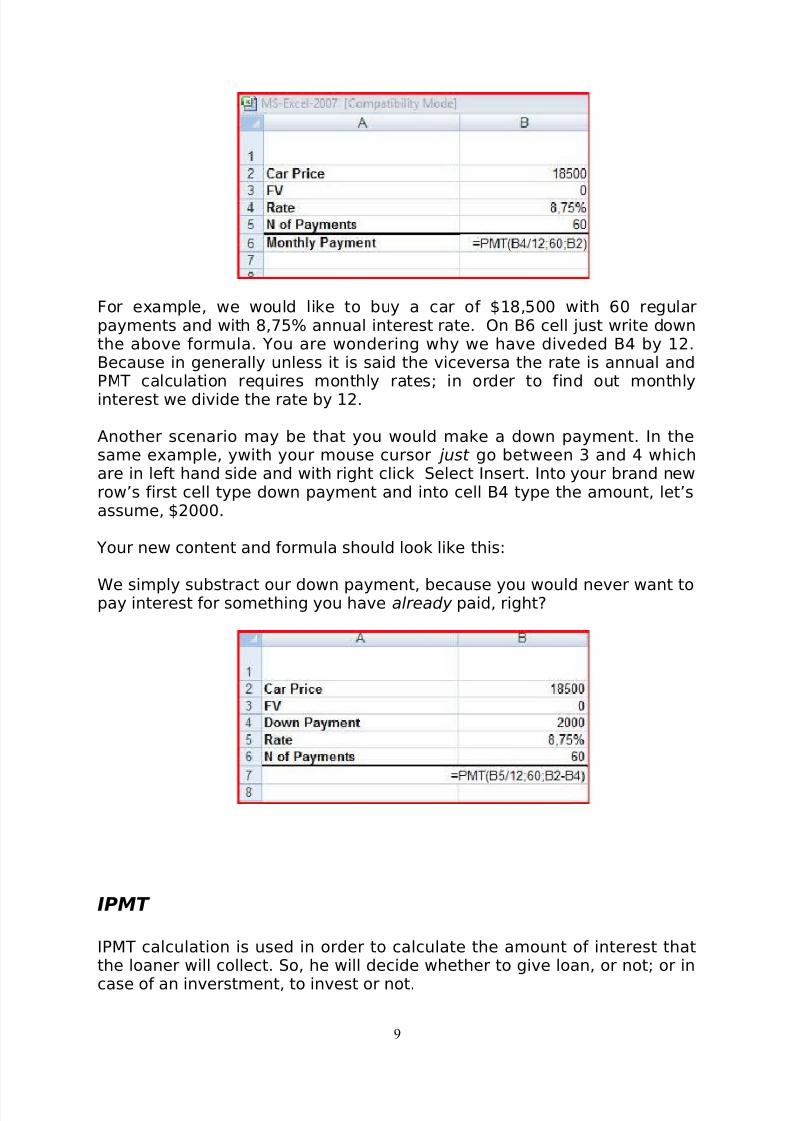
For example, we would like to buy a car of $18,500 with 60 regularpayments and with 8,75% annual interest rate. On B6 cell just write downthe above formula. You are wondering why we have diveded B4 by 12.Because in generally unless it is said the viceversa the rate is annual andPMT calculation requires monthly rates; in order to find out monthlyinterest we divide the rate by 12.

Another scenario may be that you would make a down payment. In thesame example, ywith your mouse cursor just go between 3 and 4 whichare in left hand side and with right click Select Insert. Into your brand newrow’s first cell type down payment and into cell B4 type the amount, let’sassume, $2000.

Your new content and formula should look like this:

We simply substract our down payment, because you would never want topay interest for something you have already paid, right?

IPMT

IPMT calculation is used in order to calculate the amount of interest thatthe loaner will collect. So, he will decide whether to give loan, or not; or in

case of an inverstment, to invest or not.

9



IPMT includes rate, period, n periods, present value, future value andpayment type. Let us assume that we want to buy the car mentionedabove. Just fix your data as I prepared for you and then type the formula:

As a result, you are going to find interest paid and relatively earned for aperiod which is in this case 3 for the loan that you have taken to buy abrand new car.

PPMT

This useful function helps us to define the actual amount that applies tothe balance of the loan or the investment. Here the scope is to determinethe principal payment. Type the same formula

The manner is always the same for all three functions. Do not forget todivide the interest rate by 12 if you are asked to find monthly amounts.

Auto Filter

10



Auto filter allows us to hide some of the data in our worksheet. Supposewe are having lots of data, however we want work only with some of them.It is very simple to hide the unnecessary data for us. Let’s explore it with aeasy example:

Here you can see our dataset with variousnumbers in it. In order to run Auto Filter,

just Click on a cell which contains dataand then follow the path Data < Filter <Auto Filter.

If you Click on the down arraythis box will appear asking youto filter the data. If you want to

see all of the data Check ‘SelectAll’.

You may do not want to see forexamples the ‘4’ in your data,so Uncheck the box which is inthe left hand side of ‘4’.

If your data contains blank cells,then your Auto Filter options willhave Blank and NonBlankpreferences as well as othervalues.

11



By using Auto Filter you can sort you data in an ascending or descendingway. To apply it again Click on array of Auto Filter and choose whether youwant to sort them ascending or descending.

You may also want to create custom filters. You can set your criterias up totwo. To create a filter with one criterion:

• Click on a cell

• From Data < Filter Select Auto Filter

• An array will appear at the above your data, Click on it

• Click once on the array and Select ‘Number Filters’

• On the Number Filter Menu you choose one of them based on what

you want then, Excel will run it for you. Remember to type a valuewhich designes your new dataset.

You may want to create a filter with two criteria. Just follow what I havedone below:

12



A dialog box will appear asking you to select your preferences as seenbelow.

See? It is easy and a fastest way to work with the data selected from youractual dataset.

13



Application of Table

Table of Excel allows us to see the effects of changing the data in aformula. To become clear Excel will try to find out the new solutions inaccordance with your new values.Let’s assume that we decided to take out a loan of $10000. We will paythis amount in 5 years which is equal to 60 months.

The interest rate is, let’s suppose, 9%.

By using PMT formula we can calculate our monthly payment.

However, before you take your loan you have been informed that, otherbanks give loans with 8%, and 7% consequently.

After finding out our monthly payment erase it and then type the sameformula in cell D2. This will give you the same result, now it is time tocreate our table.

14



Just write down the new entries as I did. Do always remember that Tableshould include new entries, our new values and the cell in which was typedthe PMT function!!!

After highlighting the area follow the path Data < What If Analysis < Data

Table

A small dialog box will appear asking you to determine the range for yourtable.

Column input cell should contain our actual interest rate which in this caseis 9%. It is that simple. Now it is time to see if we have do it right.

If you click on to our new results you would see a brand new formulawithin the curly brackets:

{=TABLE(,B3)}

If you type it you would not get any result because it is automaticallygenerated y Excel itself in accordance with your data and tableapplication.

Let’s examine another example by Dr. Aksen’s MS-Excel 2007 Homework.

This is actually embedded image so you can double click on it and see,what is going on, how I solve this problem by using Table function. It is

quite fun. Try it!!!

Substitute function

Substitute is a quite handy function which serves to replace a set of characters with another. Let’s take into consideration an example. I havetyped some names into cells and I want to substitute them.

15



This is an embedded image double click on it to work with thespreadsheet.Chose a cell and type the formula =SUBSTITUTE(A2;"e";"a").

It is a command to replace all the letters “e” with a.

You can give other commands. For example, you may want to replace thefirst “e” of Çeşme. For this, you should type the function=SUBSTITUTE(A3;”e”;”a”,1)

In this formula the number “1” refers to the first “e” letter. So you canplay with all the letters as you wish.

Concatenate function

Concatenate function is another handy and easy function of brillant Excel.

This is another another embedded image. I ask you to kindly double clickon it. I want to unify these 5 strings together. Type the formula=CONCATENATE(A1;A2;A3;A4;A5). You will see that the 5 strings joinedtogether.

You may want to add something that is not written in tha data set. Forexample, type the formula =CONCATENATE(A1;A2;A3;"zorlu";A4;A5)

You will be suprised that Excel unifies the cells as “Cemre Onurerin zorluExcel Odevi”

16

CEMRE - MS Excel Extra Tutorial

Documents

Transcript of CEMRE - MS Excel Extra Tutorial