Computer Physics Communications 220 (2017) 351–362

Contents lists available at ScienceDirect

Computer Physics Communications

journal homepage: www.elsevier.com/locate/cpc

almaBTE: A solver of the space–time dependent Boltzmann transportequation for phonons in structured materials

Jesús Carrete a,b,c,*, Bjorn Vermeersch a,b,*, Ankita Katre a,b, Ambroise van Roekeghem a,b,Tao Wang d, Georg K.H. Madsen c, Natalio Mingo a,b,*a Université Grenoble Alpes, F-38000 Grenoble, Franceb CEA, LITEN, 17 rue des Martyrs, F-38054 Grenoble, Francec Institute of Materials Chemistry, TU Wien, A-1060 Vienna, Austriad CMAT, ICAMS, Ruhr-Universität Bochum, 44780 Bochum, Germany

a r t i c l e i n f o

Article history:Received 13 April 2017Received in revised form 21 June 2017Accepted 26 June 2017Available online 11 July 2017

Keywords:Boltzmann transport equationThermal conductivityPhonon

a b s t r a c t

almaBTE is a software package that solves the space- and time-dependent Boltzmann transport equationfor phonons, using only ab-initio calculated quantities as inputs. The program can predictively tacklephonon transport in bulk crystals and alloys, thin films, superlattices, and multiscale structures withsize features in the nm–µm range. Among many other quantities, the program can output thermalconductances and effective thermal conductivities, space-resolved average temperature profiles, andheat-current distributions resolved in frequency and space. Its first-principles character makes almaBTEespecially well suited to investigate novel materials and structures. This article gives an overview of theprogram structure and presents illustrative examples for some of its uses.

PROGRAM SUMMARYProgram Title: almaBTEProgram Files doi: http://dx.doi.org/10.17632/8tfzwgtp73.1Licensing provisions: Apache License, version 2.0Programming language: C++External routines/libraries: BOOST, MPI, Eigen, HDF5, spglibNature of problem: Calculation of temperature profiles, thermal flux distributions and effective thermalconductivities in structured systems where heat is carried by phononsSolution method: Solution of linearized phonon Boltzmann transport equation, Variance-reduced MonteCarlo

© 2017 Elsevier B.V. All rights reserved.

1. Introduction

Thermal transport in semiconductor devices has become agrowing priority in recent years. In many technologies, the prob-lem of heat dissipation stands in the way to further progress.Phonons being the main heat carriers in semiconductors and in-sulators, clearing the path requires tackling inherently multiscaleproblems from the point of view of the fundamental physics ofvibrations in solids.

By way of example, in power electronic devices such aslight-emitting diodes (LEDs) or high-electron-mobility transistors

This paper and its associated computer program are available via the ComputerPhysics Communication homepage on ScienceDirect (http://www.sciencedirect.com/science/journal/00104655).

* Corresponding authors.E-mail addresses: jesus.carrete.montana@tuwien.ac.at (J. Carrete),

bjorn.vermeersch@cea.fr (B. Vermeersch), natalio.mingo@cea.fr (N. Mingo).

(HEMTs), the choice of substrate is crucial for the lifetime of thedevice. Lowering the temperature of the active region by 50 K canincrease a device’s time to failure by one order of magnitude [1].Thus, various generations of multilayer structured substrates [2]have been evolving in recent times in order to increase heat flow,while also satisfying other constraints such as structural integrityand cost. The difficulty in this design process is that modelingthermal transport in these structures is much more complex thaninmacroscopic systems. Theproblem inhandmay contain simulta-neous ballistic and diffusive flow of phonons, which are scatteredby complex defects such as vacancies, dislocations, interfaces, ornanoinclusions. Furthermore, itmay involve novelmaterialswhichhave not yet been thoroughly explored.

Heat transport in bulk semiconductors is now tractable froma first-principles perspective, thanks to theoretical and compu-tational advances in the last decade. Central to such treatmentsis the Boltzmann transport equation (BTE) for phonons [3] in its

http://dx.doi.org/10.1016/j.cpc.2017.06.0230010-4655/© 2017 Elsevier B.V. All rights reserved.

352 J. Carrete et al. / Computer Physics Communications 220 (2017) 351–362

space- and time-independent form. While the first practical nu-merical solution algorithm of the phonon BTE dates back to 1995[4–6], it only achieved popularity after it was combined withdensity functional theory (DFT) in 2007 [7], giving birth to ab-initiothermal transport calculations as they are understood today [8].

Key advantages of this kind of methods include their quantita-tive predictive ability, their accounting for the quantum characterof phonons, and their lack of reliance on parameterized functionssuch as interatomic potentials or semiempirical scattering rates, incontrast withmore traditional approaches like Callaway-likemod-els [9] or classical molecular dynamics simulations [10]. Examplesof successful applications of ab-initio thermal conductivity calcula-tions in recent years are too numerous to cite here, and range fromtechnologically mainstream 3D semiconductors [11] to graphene[12] and other innovative 2D materials [13]. They have been usedto provide physical insight about known behavior [14], to criticallyanalyze other models [15] and experimental data [16], and toperform high-throughput explorations across chemical space [17].Several software packages implementing these calculations areavailable, including ALAMODE [18], phono3py [19], PhonTS [20],and ShengBTE [21].

In view of the success of ab-initio thermal transport calcula-tions to date, it is highly desirable to extend them beyond thedomain of bulk systems to the multiscale situations describedabove. Unfortunately, when a dependence in position is includedin the Boltzmann transport equation, one faces the so-called ‘‘curseof dimensionality’’ [22] because of the six spatial dimensions in-volved in the problem (3D real space + 3D reciprocal space). Adirect approach to solving the BTE as a linear system, in the samespirit as for homogeneous bulk materials, is unfeasible because ofthe associated explosion in matrix sizes. Traditional Monte Carlosolvers, which have proven very useful to escape the ‘‘curse’’ inother domains ofmaterials science, are of limited use in the contextof the phonon BTE [23]. The reason is that in most situations ofpractical interest phonons are fairly close to equilibrium, meaningthat Monte Carlo methods spend most of the computational efforton characterizing the already well known equilibrium component,even though it is only the small deviation from the equilibriumdistribution that matters for thermal transport. This makes devi-ational Monte Carlo approaches [24] a much better choice. Theidea behind them is treating the equilibrium component of phonondistributions in an analytical fashion, and devoting all computa-tional resources to simulating the non-equilibrium component bysplitting it into an arbitrary number of particle-like packets whosestochastic trajectories can be traced in space and time.

In this work we describe almaBTE, a collection of solversof the Boltzmann transport equation for phonons in space- andtime-dependent settings, supplemented by a set of auxiliary pro-grams that make up a consistent framework for studying phonon-mediated heat transport in structured semiconducting systemsstarting from first principles. The 1.1 release of almaBTE featuresa new and improved implementation of all the functionality ofShengBTE [21] for bulk systems, specialized models for the in-plane and cross-plane thermal conductivity of thin films [25], avariance-reduced Monte Carlo solver of the BTE for the steady-state regime in one dimension, a general implementation of thesuperlattice models first presented in Ref. [26], and an analyticalsolver for 1D models introduced in Ref. [27].

The present paper is structured as follows. In Section 2 wedescribe the general features of almaBTE as a software packageand how its components are articulated. Then, in Section 3 weintroduce each program in the package alongwith a brief summaryof the physical and mathematical formalism behind it. We includea set of examples of application in Section 4. Finally, we summarizeour main conclusions in Section 5.

Fig. 1. ALMA 1.1 blueprint.

2. General structure of almaBTE

Fig. 1 illustrates the overall fashion inwhich the different piecesof almaBTE are organized. A from-scratch calculation starts fromthe top of the diagram, with the creation of a catalog of ‘‘effectivecrystals’’ that can be used as building blocks of more complexstructures. In this context, an ‘‘effective crystal’’ can be assignedan atomic structure and a phonon spectrum.

In terms of implementation, the information about a materialis contained in an HDF5 file [28] with a filesystem-like structurecomprising several HDF5 groups (analogous to directories):

• The /crystal_structure group contains the lattice pa-rameters, atomic positions and chemical information of thematerial.

• The /qpoint_grid group stores information about thephonon frequencies, group velocities andwave functions ona regular na × nb × nc grid in reciprocal space.

• The /scattering group can either be empty or consist ofan arbitrary collection of subgroups, each of them account-ing for a particular kind of elastic scattering. Temperature-independent scattering rates arising from a breakdown ofperiodicity are stored here. As of version 1.1 of almaBTE,there are two datasets stored in this subgroup for each

J. Carrete et al. / Computer Physics Communications 220 (2017) 351–362 353

superlattice profile, as described below. Scattering by otherkinds of crystallographic defects has already been imple-mented [29–31] and will be rolled out as part of futurereleases.

• The /threeph_processes group contains a list of al-lowed three-phonon absorption and emission processesalong with their amplitudes. Since intrinsic phonon scatter-ing is assumed to be dominated by these processes, this isthe essential ingredient required to compute the intrinsicphonon scattering rates at any temperature.

Currently, HDF5 files can be generated for three kinds ofmateri-als: single crystals, alloys treated in the virtual crystal approxima-tion (i.e., treated as statistical averages of several single crystals)and superlattices described as the combination of an alloy anda set of barriers (see the next section). As can be seen in thescheme in Fig. 1, creating an HDF5 file requires input from ab-initiocalculations, notably a geometrical description of each compoundand the second- and third-order derivatives of its potential energyat equilibrium. The format of the input files is similar to that usedin ShengBTE [21], with the addition of a new _metadata filecontaining parameters such as supercell sizes. Moreover, an XMLinput file for the HDF5 builders needs to be written to instruct theprograms as to how to combine the inputs to build a description fora single material. In the case of an alloy this entails providing a setof concentrations, while a superlattice can be described in terms ofthe composition of each of its layers. Examples of all required inputfiles can be found in the almaBTE distribution. In order to promotecollaboration and avoid duplication of work, we have started arepository of publication-quality input files from ab-initio calcu-lations at http://www.almabte.eu. The database currently coversabout twenty compounds of scientific and technological interest.Users are encouraged to use the files in their own research and tocontribute descriptions of new compounds.

The HDF5 files can be fed to the remaining programs, classifiedas ‘‘thermal property explorers’’ and ‘‘BTE solvers’’ in Fig. 1, anddescribed in detail below. Each of them requires its own XMLinput file, providing it with a description of the operations to becarried out. The output is stored in text-based formats that are bothreadable and easily parseable by common data analysis software.

almaBTE has been designed with portability in mind. The codeis written in standard C++11 making heavy use of the Boostlibraries, and using Eigen for linear algebra operations. The buildsystem uses CMake to take care of dependencies automatically. APIand user documentation are included with the code, along with asuite of unit tests built using the Google Test library. The codeis regularly built and tested with the CLang and g++ compilerson Linux and macOS. Furthermore, we have built a containerizedversion using Docker that can be used on an even wider rangeof platforms, including Microsoft Windows. It is also available fordownload from the web site.

The performance-critical regions of the code have been par-allelized using MPI through the Boost::MPI wrappers. Severalcentral parts of the algorithms are ‘‘embarrassingly parallel’’ bynature, and can be distributed over processors with minimal needfor communication. Specifically, the calculations of phonon fre-quencies andwave functions, the search for allowed three-phononprocesses and the calculation of scattering matrix elements can beefficiently parallelized over wavevectors. In non-I/O-constrainedcalculations, the performance of almaBTE has been found to scalealmost linearly at least up to 512 cores.

3. Programs included in the package

3.1. VCAbuilder

This binary is a general-purpose builder of HDF5 files for singlecrystals and alloys treated in the virtual crystal approximation(VCA).

For a single crystal, VCABuilder reads the structural parame-ters (lattice vectors, elements and positions) from a POSCAR filein the format employed by the VASP [32–35] density functionaltheory (DFT) package. Next, it reads the set of second derivativesof the potential energy of a supercell with this crystal structurefrom a FORCE_CONSTANTS file in the format employed by thephonopy [36] lattice dynamics software. Those elements are alsoknown as harmonic, or second-order, interatomic force constants(IFCs). It then creates a regular, Γ -centered na × nb × nc grid inreciprocal space and, for each point in the grid, builds the dynami-cal matrix based on the atomic positions and harmonic IFCs. If thecompound under study contains polar bonds, this information canbe complementedwith values of its dielectric tensors and the Borneffective charges [37] of each atom. Those are read from a BORNfile similar to the ones used by phonopy, and used according tothe mixed-space algorithm proposed by Wang et al. [38,39]. Bydiagonalizing the corrected dynamical matrix at each wavevector,the program obtains a set of allowed vibrational frequencies and acorresponding set of phonon wave functions describing the polar-izations of each atom in each mode.

VCAbuilder then performs a search for allowed three-phononprocesses among all the vibrational modes on that regular grid.Let us use generalized indices k, k′ . . . here and in the remainingof this work to label both the wavevectors and the polarizations(branches) of phonons. Two kinds of three-phonon processes arepossible: absorption (+) processes where two phonons k and k′ co-alesce into a single phonon k′′ , and emission (−) processes, wherea single incident phonon k scatters into two outgoing phonons.For a three-phonon process to be allowed, it must preserve bothenergy and momentum. Conservation of momentum is triviallyenforced on a regular grid, simply by performing the search onlyamong phonons for which q ± q′

= q′′, where the equality mustbe understood in a modular sense, i.e., taking into account theperiodicity of reciprocal space. In contrast, angular frequenciesω are not uniformly distributed, meaning that in general modessatisfying the condition ωk ± ωk′ = ωk′′ for the conservation ofenergy will not be sampled by the grid. The solution adopted inalmaBTE is based on a linear extrapolation of angular frequenciesaround each grid point using the calculated group velocities, as de-scribed in Ref. [40] and previously implemented in ShengBTE [21].In practice this translates into a parameter-free locally adaptivedensity estimation schemewith a Gaussian kernel. However, usershave thepossibility to artificially reduce thewidth of eachGaussianby a constant factor in order to speed up the calculation. Althoughthis shortcut often leads to very little loss of accuracy, this shouldalways be carefully checked.

For each allowed three-phonon process, the program then com-putes a scattering amplitude using the formulas in Ref. [21]. Theessential ingredient is a set of third-order derivatives of the po-tential energy of a supercell of the crystal, i.e., the third-order oranharmonic IFCs. Those are read from a FORCE_CONSTANTS_3RDfile in the format used by ShengBTE.

The number of allowed three-phonon processes for a typicalgrid is very high (106

− 1012) which leads to high requirementsof memory and CPU time. Such process searches are optimized byusing the rotations from the space group of the crystal to determinethe quotient group of the wavevectors in the grid. A smaller set ofwavevectors, which we term the ‘‘irreducible wavevectors’’ is thenbuilt by taking an arbitrary representative from each equivalenceclass in the quotient group. To do this we rely on the informationabout the space group of the crystal provided by spglib. We thenrestrict the search to three-phonon processes in which the firstphonon (k) has an irreducible wavevector. Any property can beextrapolated from the irreducible set to the full wavevector gridby using the rotation operations and taking into account its tensorcharacter (scalar, vector, etc.). In particular, relaxation times are

354 J. Carrete et al. / Computer Physics Communications 220 (2017) 351–362

scalar values, and the phonon populations can be parameterizedin terms of a vector quantity Fk as detailed in Ref. [21].

In order to build a description of an n-ary alloy, VCABuilderneeds the same set of input files (POSCAR, _metadata, FORCE_CONSTANTS, FORCE_CONSTANTS_3RD and possibly BORN) foreach of the n components. Furthermore, each of those componentsmust contain the same number of elements, with identical sto-ichiometry and the same crystal structure, so that a one-to-onemapping can be established between the crystallographic sites ofeach structure. VCABuilder computes effective parameters fora virtual crystal representing the alloy, using simple arithmeticaverages φVC =

∑ixiφi, where xi is themole fraction of component

i (normalized so that∑

ixi = 1), and φi can stand for a latticevector, an atomic coordinate, a second- or third-order IFC, thedielectric tensor or a Born effective charge. This relatively crudeapproximation has the advantage of not requiring any further ab-initio calculations beyond those for the pure components of thealloy, no matter what the concentrations are, and has been shownto afford reasonable results [41]. On the other hand, its limitationsmust be borne in mind as it does not account for correlations, localrelaxations or changes in electronic structure due to alloying.

The compositional disorder present in alloys increases the prob-ability of elastic phonon scattering. This is taken into account bytreating the alloy as a random mass perturbation upon the ref-erence virtual crystal. Elastic scattering amplitudes are computedusing the formula derived by Tamura [42], in complete analogy tomass disorder scattering in a single crystal. As described below,the ingredients in this treatment are the phonon spectrum of thevirtual crystal and the standard deviation of the mass at eachcrystallographic site.

3.2. superlattice_builder

This component of almaBTE can create HDF5 files containingdescriptions of the phonon spectrum and scattering propertiesof binary superlattices. An idealized superlattice consist of a re-peated alternating sequence of two different compounds, A andB, whose lattices need to be reasonably well matched to preventdislocations. Additionally, superlattice_builder requires thatthe structures of the two compounds satisfy the conditions of thevirtual crystal approximation described above. A period of the su-perlattice is specified by a number of layersNlayers and a set ofmolefractions xi

Nlayersi=1 describing the concentration of component A in

each layer, with component B present, correspondingly, in molefractions 1 − xi

Nlayersi=1 . For an ideal ‘‘digital’’ profile, this consists

of either 0 or 1 values for each layer. Segregation during growthleads to composition profiles that can differ markedly from thedigital profile. A crucial difference between the digital profile andthe segregated one is that the former is completely homogeneousin the directions parallel to the SL layers, whereas the latter con-tains local compositional disorder in all three spatial directions.This interplay between 1D and 3D compositional variation has animportant effect on phonon scattering.

Wemodel a superlattice as a periodic perturbation upon a refer-ence virtual crystalwithmole fraction

∑ixi/Nlayers of componentA.

The perturbation contains two contributions, from mass disorderand frombarriers. The former accounts for the randomdistributionof components A and B within each layer of the superlattice, andis modeled using Tamura’s formula with the compositions xi and1 − xi in each layer i. The latter depends only on the coordinatealong the growth direction, and represents the effect of the averagemass profile scattering due to nanostructuring. This methodologywas first introduced in Ref. [26] and validated by reproducingexperimental thermal conductivity measurements on Si/Ge super-lattices.

The barrier contribution to scattering comes from an intenseenough perturbation as to require a fully converged treatmentin the framework of perturbation theory. More specifically, theperturbed phonon wave functions are different enough from theunperturbed ones as to cause a breakdown of Fermi’s golden rule(or, equivalently, the Born approximation). Since the scatterer istranslationally invariant in the two directions parallel to the super-lattice layers, phonons scattered by barriers preserve the parallelcomponents of their wavevectors: an incident state can only bescattered to other states with the same parallel wavevector. Henceit is convenient to use a hybrid real/reciprocal space represen-tation: the direction perpendicular to the superlattice layers istreated in real space, whereas the translationally invariant direc-tions parallel to the layers are considered in reciprocal space. Thecontribution to the total elastic scattering rates from barriers isobtained using the optical theorem:

τ−1barrier = −

1ωb

(q⊥, q∥

)ℑ⟨q⊥, q∥, b

t+(q∥

) q⊥, q∥, b⟩. (1)

Here, q∥ stands for the conserved parallel component of thewavevector, q⊥ for the component perpendicular to the layers, b forthe phonon branch index, and t+ for the causal t matrix, obtainedfrom the causal Green’s function g+ as:

t+(q∥

)=

[1 − Vg+

(q∥

)]−1V , (2)

where V is the perturbation matrix describing the barrier. Notethat, in the spirit of the virtual crystal approximation, superlat-tice_builder models the perturbation as a periodic change inmass and neglects the possible change in force constants. Eachcomponent of the causal Green’s function involves an integral inthe non-conserved component of the wavevector:

g+

(i,α),(j,β)

(q∥, ω

2)= lim

ϵ→0+

∑b

1length [L (q⊥)]

×

∫L(q⊥)

⟨i, α|q⊥, q∥, b⟩⟨q⊥, q∥, b|j, β⟩

ω2 − ω2b

(q⊥, q∥

)+ iϵ

dq⊥. (3)

The integration region L (q⊥) is the segment in reciprocal spacedetermined by the intersection of the reciprocal-space unit celland the line passing through

(q⊥, q∥

)in the supercell growth

direction. In contrast to the 2D and 3D cases, this 1D Green’s func-tion contains drastic divergences at any point where the branchesdo not have a continuous derivative. This includes the physicaldivergences at the band edges, but also artifactual ones wherevertwo linear segments of a bandmeetwith different slopes. Hence, anapproach based on linear interpolation of the bands between eachpair of points in a grid (analogous to the tetrahedron method [43]in 3D) becomes numerically problematic as the number of gridpoints is increased. superlattice_builder implements a newapproach to this integral in the analytically correct ϵ → 0+ limit.Since the group velocities are also available during the calculation,we build a cubic interpolation of each band, with continuousderivatives throughout the whole L (q⊥) segment. The contribu-tions to the Green’s function from each sub-segment in the regulargrid can still be expressed analytically; the increasedmathematicalcomplexity is more than compensated by the drastically reducednumber of points that need to be included in the grid since thepiecewise cubic polynomial provides amuch better approximationto the real bands than a set of linear segments. Detailed formulasare provided in the Appendix.

After computing themass-disorder and barrier contributions toscattering, superlattice_builder stores them as two separatesubgroups of the /scattering HDF5 group. A unique suffix isgenerated for each superlattice, so that several different profilescan be stored in the same file.

J. Carrete et al. / Computer Physics Communications 220 (2017) 351–362 355

3.3. kappa_Tsweep

This executable provides efficient computations of the thermalconductivity κ(T ) versus ambient temperature. Unlike Sheng-BTE, the allowed three-phonon emission/absorption processes andassociated scattering matrix elements V±

k k′ k′′ do not need to berecomputed since inalmaBTE this information is stored in anHDF5file (see previous sections). This renders the evaluation of thermalbulk properties over a large number of ambient temperatures afairly quick task. After reading the HDF5 file from disk, the pro-gram precomputes the total temperature-independent 2-phononscattering rates 1/τ2ph. All that remains is then to compute the 3-phonon scattering rates at each of the temperature values usingthe formulas detailed in Ref. [21], obtain the total scattering rates1/τ = 1/τ2ph +1/τ3ph, and evaluate the bulk thermal conductivityas described below.

One of the contributions to 1/τ2ph comes from mass-disorderscattering, either due to the presence of several isotopes in thecrystal or to alloying [42]:

τ−1k,m.d. =

πω2k

2

∑k′,i

σ 2 (mi)

⟨mi⟩2

∑α

⟨i, α|k⟩⟨k′|i, α⟩

2

δ (ωk − ωk′) . (4)

Here, i runs over crystallographic sites in a single unit cell, and⟨mi⟩ and σ 2 (mi) are the arithmetic mean and the variance of thedistribution of masses at site i, respectively.

In case additional sources of elastic scattering, e.g. dislocations,are present, the corresponding datasets can be read from the inputHDF5 file and added on top of mass-disorder scattering to obtainthe total 1/τ2ph. The case of superlattices is special, since mass-disorder scattering is computed in a layer-by-layer fashion. Hence,for superlattices the result of Eq. (4) is replaced by, and not simplyadded to, the elastic scattering rates read from the file.

3.3.1. Relaxation time approximationUnder the relaxation time approximation (RTA), the component

of the thermal conductivity tensor along Cartesian axes α and β isimmediately obtained as

κα,β =

∑k

Ckvα,kvβ,k

|vk|Λk. (5)

In this equation, Ck is themode contribution to C(T ), the volumetricheat capacity, v the group velocity, andΛ(T ) = |v| τ (T ) the meanfree path. The sum over k must be interpreted as the combinationof a sum over branches and an average over the Brillouin zone. Thesame convention applies for the remainder of the manuscript.

3.3.2. full BTE computationsIt is also possible to solve the linearized BTE for bulk media

subjected to a temperature gradient while fully accounting forall scattering terms. This is achieved through a linear system ofequations (described in detail in Ref. [21]) that takes the form

AF = B (6)

whose solution comprises a Cartesian vector Fk =(Fk,x, Fk,y, Fk,z

)for each phonon mode k. Those vectors act as generalized meanfree paths in the expression of the thermal conductivity tensor:

κα,β =

∑k

Ck vk,α Fk,β . (7)

In ShengBTE, the system (6) contained unknowns for every pointin the wavevector grid and was solved iteratively, starting fromthe RTA solution Fk,α = τk · vk,α as initial guess. Here, we exploitrotational symmetries to rewrite the system solely in terms ofunknowns pertaining to irreducible grid points, and then solve thissystem directly with Eigen routines.

Fig. 2. In-plane thin film transport: (a) geometric configuration, (b) phonon trajec-tory involved in evaluating conductivity suppression function.

3.4. kappa_crossplanefilms, kappa_inplanefilms

These executables enable efficient assessment of 1D thermaltransport in thin films for both in-plane (∥) and cross-plane (⊥)configurations. The effective RTA thermal conductivity in a film ofthickness L is evaluated as

κeff(L) =

∑k

Sk(L) Ck ∥vk∥Λk cos2ϑk. (8)

here S is a ‘‘suppression function’’ that accounts for the additionalphonon scattering induced by the film boundaries and ϑ is theangle between the group velocity and the transport axis. It isimportant to note we evaluate the wavevector-resolved S on amode-by-mode basis and thereby carefully account for any crystalanisotropies. This can be particularly important when analyzingnon-cubic crystals. Most literature resolves S by phonon frequencyunder the assumption of isotropic phonon dispersions.

3.4.1. In-plane transportThe in-plane geometry is described by two Cartesian vectors:

the film normal n, and an orthogonal vector u along which thethermal transport is to be evaluated (Fig. 2a).

The film boundaries are assumed to possess the same spec-ularity 0 ≤ p ≤ 1 for all phonon frequencies/wavelengths.For algebraic convenience, we carry out our computations in atransformed coordinate system inwhich the film normal is alignedwith the new z axis. This is easily achieved by performing a 3Drotation of the original coordinates with rotation matrix

R =

[cosφ cos θ sinφ cos θ − sin θ− sinφ cosφ 0

cosφ sin θ sinφ sin θ cos θ

](9)

in which φ and θ are respectively the azimuthal and polar an-gles of the film normal in original coordinates, i.e. n/|n| =

(cosφ sin θ, sinφ sin θ, cos θ). Quantities expressed in trans-formed coordinates will be marked with a ˆ symbol; for example,the rotated phonon group velocities read v ≡ Rv. The suppressionfactor S of an individual phonon mode now follows from thesame reasoning that underpins the familiar Fuchs–Sondheimerformalism, albeit before any integrations over solid angle havebeen applied. Specifically, working backwards from Eq. (11.5.3) inRef. [3] we have

S∥ =1L

∫ L

0

[1 −

(1 − p) exp(−∥r − rB∥/Λ

)1 − p exp

(−∥rB − rB′∥/Λ

) ]dz. (10)

The meaning of the various points along the phonon trajectory isillustrated in Fig. 2b. We obtain for any vz = 0

∥r − rB∥Λ

=sgn(vz) z +

12 [1 − sgn(vz)]LK · L

(11)

∥rB − rB′∥

Λ=

1K

(12)

356 J. Carrete et al. / Computer Physics Communications 220 (2017) 351–362

where we introduced the effective Knudsen number [44]

K =(vz/∥v∥) ·Λ

L=Λz

L. (13)

The integration (10) yields

S∥ =1 − p exp

(−

1K

)− (1 − p) K

[1 − exp

(−

1K

)]1 − p exp

(−

1K

) . (14)

Notice that S∥(K → 0) = 1 regardless of the specularity p.This confirms the recovery of bulk transport in very thick films(L → ∞), and correctly signals that phonons which never interactwith the film boundaries (vz = 0) contribute their full nominalconductivity regardless the film thickness.

3.4.2. Cross-plane transportThe cross-plane configuration can be fully specified by a single

Cartesian vector, since the transport is evaluated along the filmnormal: u ≡ n. Here the film boundaries are considered to act asperfectly absorbing black bodies. The suppression function can becompactly written as

S⊥ =1

1 + 2K(15)

where the Knudsen number can be simply evaluated as K =

Λ |cosϑ |/L without the need for coordinate transforms. Although(15) is not rigorously exact, we have shown in prior work [25]that this suppression function reproducesMonte Carlo simulationsof the effective conductivity within a few percent and is closelycompatible with semi-analytic solutions of the BTE in a finite do-main. almaBTE can furthermore perform an accurate parametricfitting of the computed κ⊥(L); details on these compact models areavailable in Ref. [25].

3.5. Cumulativecurves

This executable reveals the contributions of phonon modesto bulk heat capacity and thermal conductivity. In particular, itcomputes curves of the form

CΣ (X∗) =

∑Xk ≤ X∗

Ck, κΣ (X∗) =

∑Xk ≤ X∗

Ck ∥vk∥Λk cos2ϑk (16)

resolved by phonon parameter X which can be mean free pathΛ;relaxation time τ ; ‘‘projected’’ mean free path Λ|cos θ |, which asdescribed above plays a central role in cross-plane film transport;frequency ν; angular frequencyω = 2πν; or energy E = hν = hω.

3.6. transient_analytic1d

Theanalytic1dmodule inalmaBTE enables exploration of 1Dtime-dependent phonon transport in infinite bulk media. Specif-ically, the module provides semi-analytic solutions of the singlepulse response of the Boltzmann transport equation under therelaxation time approximation (RTA-BTE). The heat flow geometryis taken as one-dimensional, meaning that the thermal field onlydepends on one Cartesian space coordinate x.

Let us consider a planar heat source located at x = 0 that attime t = 0 injects a pulse of thermal energy with unit strength1 J/m2 into themedium. As is customary, we assume that the inputsource energy gets distributed across the various phonon modesaccording to their contributions to the heat capacity. The RTA-BTEdescribing the transient evolution of the deviational volumetricthermal energy g(x, t) of a phonon mode then reads

∂gk∂t

+ vx,k∂gk∂x

= −gk − Ck∆T

τk+

Ck∑Ckδ(x) δ(t). (17)

Subscripts x indicate quantities measured along the thermal trans-port axis. The equation needs to be complemented by a closurecondition expressing the conservation of energy:∑

k

1τk

(gk − Ck∆T ) = 0. (18)

Analytic solutions of the stated 1D problem have been previouslyderived in transformed domains, first for isotropic media [45] andthen generalized to crystals with arbitrary anisotropy by several ofthe almaBTE developers [27]. In Fourier–Laplace domain (x, t) ↔

(ξ, s) themacroscopic deviational energy density P ≡ (∑

Ck)×∆Tis given by

P(ξ, s) =

∑CkΞk(ξ, s)∑

(Ck/τk) [1 −Ξk(ξ, s)](19)

in which Ξk(ξ, s) =1 + sτk

(1 + sτk)2 + ξ 2Λ2x,k

(20)

where Λx ≡ |vx| τ as usual. The analytic1d module computesseveral quantities of interest by inverting the solution (19)–(20)semi-analytically to real space and time, as described below.

3.6.1. Temperature profiles∆T (x, t)Fourier–Laplace inversion of the thermal fields can be greatly

simplified if we limit ourselves to weakly quasiballistic regimes|s|τ ≪ 1 for which we have

P(ξ, t) ≃ exp [−ψ(ξ ) t] (21)

with ψ(ξ ) =

∑ Ck ξ2Λ2

x,k

τk[1 + ξ 2Λ2x,k]

/∑ Ck

1 + ξ 2Λ2x,k. (22)

This solution ignores purely ballistic transport effects, but offersexcellent performance at temporal scales exceeding characteristicphonon relaxation times (typically 1–10 ns). To perform Fourierinversion to real space

P(x, t) =1π

∫∞

0P(ξ, t) cos(ξx) dξ (23)

we first execute a piecewise second-order Taylor series expansionover consecutive ξ intervals

exp[−ψ(ξ ) t] ≃ A0,n(t) + A1,n(t) ξ + A2,n(t) ξ 2 (24)

which can then be integrated fully analytically:

x = 0 :

∫(A0 + A1ξ + A2ξ

2) cos(ξx) dξ = −2A2 sin(ξx)

x3

+(A1 + A2ξ ) cos(ξx)

x2+

(A0 + A1ξ + A2ξ2) sin(ξx)

x. (25)

Downscaling this solution by the bulk heat capacity yields thedesired temperature profile:∆T (x, t) = P(x, t)/

∑Ck.

3.6.2. Source response∆T (x = 0, t)Experiments typically have no access to the internal thermal

fields but can only probe the temperature rise generated at the heatsource itself. The latter can be computed by evaluating the Fourierinversion (23) at x = 0 using linear quadrature. Limiting ourselvesagain to quasiballistic regimes, we find

P(x = 0, t) ≃

∑n

[exp(−ψn t) − exp(−ψn+1 t)] ∆ξn(ψn+1 − ψn) t

(26)

in which ψj ≡ ψ(ξj) and∆ξj = ξj+1 − ξj.

3.6.3. Mean square displacement σ 2(t) =∫x2P(x, t)dx

The evolution of the thermal mean square displacement, de-fined as the variance of the deviational energy distribution, is

J. Carrete et al. / Computer Physics Communications 220 (2017) 351–362 357

readily obtained in Laplace domain through moment generatingproperties:

σ 2(s) = −∂2P(ξ, s)∂ξ 2

ξ=0. (27)

From the general BTE solution (19)–(20) we find

σ 2(s) =2∑κk/(1 + sτk)2

s2∑

Ck/(1 + sτk)(28)

where κk = Ck |vx,k|Λx,k is the phonon thermal conductivity. Notethat the expression (28) applies to all time scales; in particular, itis also valid in purely ballistic and strongly quasiballistic transportregimes. Finally, we evaluate the time domain counterpart σ 2(t)through numerical Gaver–Stehfest Laplace inversion [46].

3.7. steady_montecarlo1d

Thesteady_montecarlo1dmodule enablesMonte Carlo sim-ulations of steady-state thermal transport in 1D multilayeredstructures with isothermal boundary conditions.

The computational algorithm is based on the variance-reduceddeviational techniques introduced by Peraud and Hadjiconstanti-nou [23,24,47] for numerical solution of the RTA-BTE. However,we emphasize again that our computations utilize first-principlesphonon properties that are wavevector-resolved. Prior publica-tions often employed parameterized dispersions and/or scatteringrates, therefore lacking predictive power for novel materials notyet experimentally characterized. Moreover, most formulationsspecify phonon properties as a function of frequency, which be-comes highly problematic in anisotropic crystals.

The central idea of variance-reduced methods for solving thephonon BTE is to approximate gk, the nonequilibrium componentof the energy distribution for each phonon mode, by the sumof a predefined number of delta functions, all of them with thesame energy and each with a well defined position. The stochastictrajectories of these energy packets are then tracked in order toreconstruct gk. The simulation proceeds very much like a conven-tional particle-based Monte Carlo, leading to the label of ‘‘devia-tional particles’’ for these packets. However, it is important to keepin mind that deviational particles are neither phonons nor evenabstract bundles of phonons, but corrections to the analytic Bose–Einstein reference distribution. As such, a particle can be eitherpositive or negative, depending on whether it was launched froma hot or a cold reservoir respectively.

steady_montecarlo1d implements a specialized version ofvariance-reduced Monte Carlo that allows simulating the steady-state regime directly without the need for an equilibrationphase [23]. This variation on the original idea exploits the timetranslation invariance of the ensemble of possible trajectories dueto the stationary character of steady-state phonon populations.Based on this property, deviational particles are taken to representfixed amounts of power, instead of fixed amounts of energy.

The simulations are carried out under the linearized regime.This assumes that the temperature deviations ∆T are sufficientlysmall that the phonon properties of each constituting material canbe treated as location independent and equal to those evaluatedat the reference temperature Tref = (Thot + Tcold)/2. Under theseconditions, deviational particles act completely independently,allowing efficient and straightforward parallellization, and theirtrajectories x(t) can be readily evaluated in a robust way withoutrequiring any spatial or temporal discretizations.

We now take a closer look at the various events a particle mayencounter during its computational lifetime (Fig. 3).

Fig. 3. Schematic overview of possible events encountered by deviational particlesin Monte Carlo simulations. (For interpretation of the references to colour in thisfigure legend, the reader is referred to the web version of this article.)

3.7.1. Emission from a thermal reservoir (launch event)The deviational intensity [W/m2] injected into the structure by

an isothermal reservoir at temperature Tiso is given by

Iiso =hV

∑k

(vk · n)H(vk · n)ωk [fBE(ωk, Tiso) − fBE(ωk, Tref)] (29)

where H is the Heaviside function and n denotes the outwardlypointing normal vector. Each particle randomly selected to beemitted from the hot or cold reservoirwith respective probabilitiesphot = |Ihot|/(|Ihot| + |Icold|) and pcold = 1 − phot, while theassociated phonon mode is drawn at random with probabilityproportional to (vk · n)H(vk · n)ωk |fBE(ωk, Tiso) − fBE(ωk, Tref)|. Theprocess is illustrated by orange arrows in Fig. 3. The + and − labelson particles emitted from the hot and cold reservoirs, respectively,denote the sign of their contributions to the deviational energy.

3.7.2. Advection stepsA provisional travel time χ is drawn from an exponential dis-

tribution with mean τk, and the particle provisionally moved over∆x = χvx. If the advection step does not traverse any layer bound-aries, the particle is moved to the new location and undergoes in-trinsic scattering (blue in Fig. 3). Otherwise, the particle ismoved tothe boundary, its travel time adjusted accordingly, and undergoeseither interface scattering (green) or reservoir absorption (pink).

3.7.3. Intrinsic scatteringA new phonon mode is drawn with probabilities proportional

to Ck/τk, afterwhich the simulation proceedswith a new advectionstep.

3.7.4. Interface scatteringParticles that reach the interfaces between dissimilar materials

M1 and M2 are transmitted/reflected according to a diffuse mis-matchmodel that allows for elasticmode conversions. Specifically,the particle is assigned a new phonon mode drawn from distribu-tion (vM

k · n)H(vMk · n)GM (ωk)/(VMNM

tot) where M ∈ M1,M2, nis a normal vector pointing away from the interface, G denotes theGaussian regularization of the energy conservation δ(ω − ωk) andNtot = NA × NB × NC × Nbranches is the total number of availablephonon modes. This is again followed by a new advection step.

3.7.5. Absorption at a thermal reservoir (termination event).A particle completes its trajectory upon reaching an isothermal

reservoir at either end of the structure. Its contributions to thetemperature profile and heat flux are evaluated with the proce-dures described below, after which the simulation proceeds withthe launch of the next particle.

3.7.6. Evaluation of temperature profileIntroducing a series of consecutive bins ofwidthw enables us to

evaluate a deviational temperature profile∆T (x) at the bin centers

358 J. Carrete et al. / Computer Physics Communications 220 (2017) 351–362

Fig. 4. Processing of a particle trajectory segment to evaluate its contribution to thedeviational temperature profile.

as follows. Each particle represents a deviational intensity

ρ = ±|Ihot| + |Icold|

Nparticles(30)

where the sign depends on which isothermal reservoir emittedthe particle as mentioned earlier. The trajectory of each of theseparticles consists of one or more linear segments, each of whichmoved the particle inside the structure from some depth xi at sometime ti to a depth xf at a time tf . The bin edges further divide thesegments into subsegments that span lengths |∆xn|, |∆xn+1|, . . .across bins n, n + 1, . . . respectively (Fig. 4).

The contribution to the steady-state deviational temperature inbin l is now evaluated as1wCl

(tf − ti)ρ|∆xl|

|xf − xi|(31)

where Cl is the bulk volumetric heat capacity of the material towhich the l th bin belongs.

3.7.7. Evaluation of net and spectral heat fluxDetermining the net heat flux only requires observing suc-

cessful particle crossings. Specifically, the heat flux in each bin isfound by accumulating ±|ρ|/Ltot each time a trajectory segmenttraverses the bin center, where the + sign is used for motion ofpositive (negative) particlemoving in the hot-to-cold (cold-to-hot)direction and the − sign for the opposite cases, and Ltot is thetotal structure thickness. Barring stochastic fluctuations inherentto the Monte Carlo methodology, the flux profile is completelyflat across the structure, due to the 1D and steady-state characterof the simulation. Bin crossings can additionally be resolved interms of the angular phonon frequency the particle was associatedwith at the time of the crossing, to reveal the spectral heat fluxqω(x). Rather than using simple binning with respect to ω, whichyields a fairly crude and noisy result, we employ locally adaptivekernel density estimation with Γ distributions that accounts forthe central frequency of the phonon mode and smoothens out theartifacts introduced by our discrete reciprocal-space grid.

3.7.8. Evaluation of effective thermal metricsOnce the net heat flux qnet is known, we can easily derive the

apparent thermal conductivity of the entire structure:

κeff =qnet

(Thot − Tcold)/Ltot. (32)

Alternatively, we can also express the thermal performance interms of the effective resistivity/conductance:

reff ≡ g−1eff =

Thot − Tcoldqnet

=Ltotκeff

(33)

4. Examples of application

4.1. Thermal conductivity of bulk materials

Fig. 5 shows computed output for diamond, Si and wurtziteGaN. Except for the first material, where proper treatment ofnormal scattering processes is crucial [Eq. (7)], the RTA offersaccurate conductivities within ∼5% of full BTE counterparts formost common semiconductors.

Fig. 5. Temperature dependence of bulk thermal conductivity.

Fig. 6. β-phase gallium (III) oxide (β-Ga2O3) crystal. (a) Unit cell, (b) computedphonon spectrum and density of states.

4.2. Effective thermal conductivity of thin films

The most stable phase of gallium (III) oxide (Ga2O3) is the so-called β phase [48], with a monoclinic structure and 10 atomsper primitive unit cell (Fig. 6a shows the conventional 20-atomcell). This relatively complex structure shows significant thermalanisotropy [49] and provides a good test case for full-spectrum thinfilm calculations.

DFT calculations for this compound were performed with thePBEsol exchange–correlation functional as implemented in VASP.We employed the finite-temperature methodology described inRef. [50] to obtain the 2nd- and 3rd-order IFCs at 300 Kwith a 3×3×3 supercell and 14th nearest neighbor cutoff, using 100 displacedconfigurations for each cycle, without taking into account anymodification of the structure with respect to the DFT ground state.The resulting phonon spectrum and DOS are illustrated in Fig. 6b.

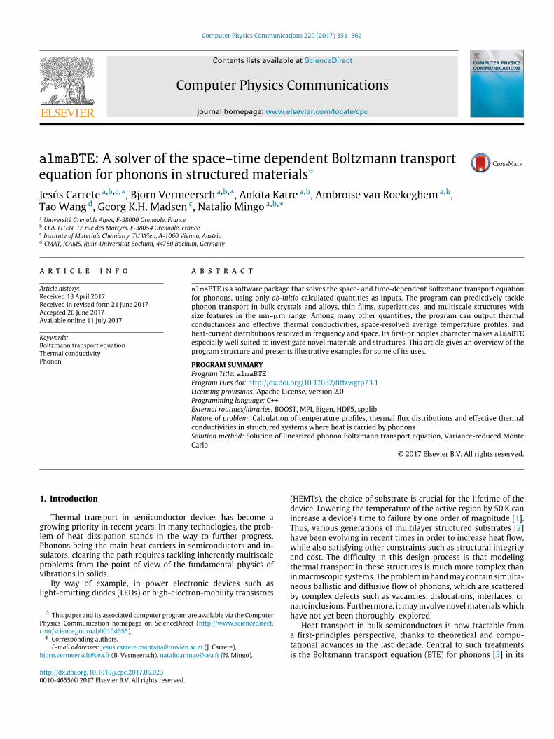
Fig. 7 shows the thin film conductivities computed for a 12×12 ×12 wavevector grid. We note that due to the low symmetryof the β-Ga2O3 crystal structure a large number of three-phononprocesses must be considered, resulting in an HDF5 file more than8 GiB in size.

At room temperature, two different values of the bulk ther-mal conductivity along the most conductive (010) axis are now

J. Carrete et al. / Computer Physics Communications 220 (2017) 351–362 359

Fig. 7. Apparent thin film thermal conductivity in β-Ga2O3 .

coexisting in the literature [49].1 We find that the bulk thermalconductivity at room temperature is close to 21 W/m/K alongthe most conductive (010) axis. This is in agreement with theexperimental measurements of Ref. [52]. In addition, we remarkthat the value of 27 W/m/K found in Ref. [51] deviates from thegeneral trend that can be deduced from their measurements atother temperatures. Our results are also in line with previouscalculations [53] performed with ShengBTE [21], except for the(001) direction for which we find a value much closer to theexperimental measurements [51] — probably because we use alarger supercell and cutoff.

4.3. Cumulative thermal conductivity curves

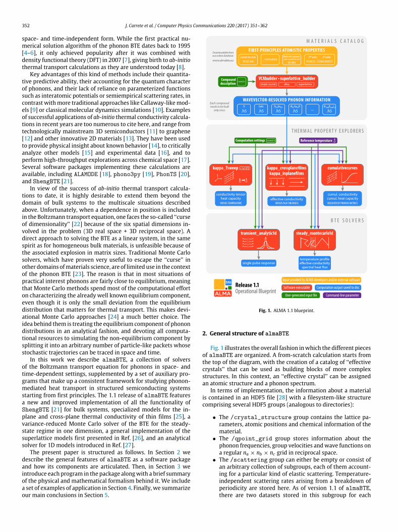
Fig. 8 shows cumulative curves resolved by mean free path andenergy computed for wurtzite GaN, AlN and Al0.5Ga0.5N with 24×24 ×24 wavevector grids.

4.4. Single pulse response of semi-infinite substrates

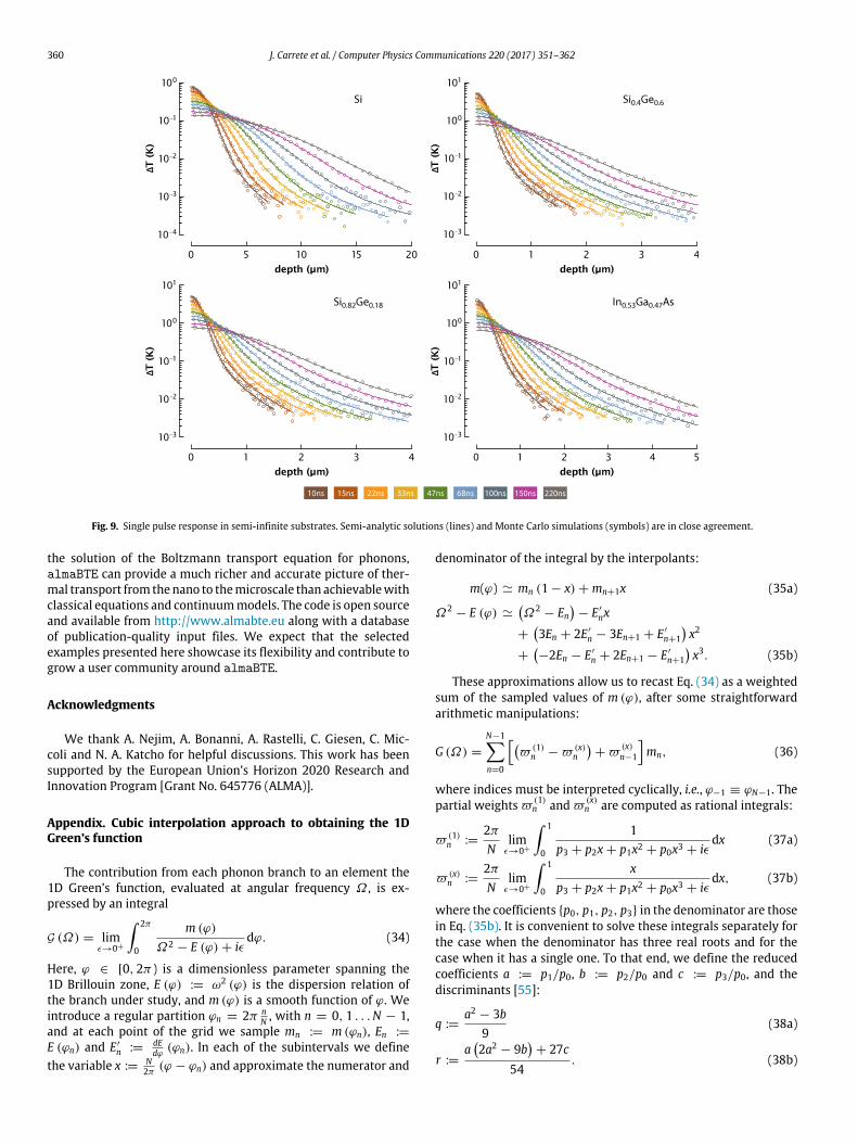
We have computed the single pulse response over the timerange 10 ns–220 ns in several semi-infinite substrates by doublingthe transient_analytic1d output results. Strictly speakingthis ‘‘method of images’’ is only valid for a perfectly specular topsurface. However, Monte Carlo simulations with surface specular-ity p = 0.5 show that the semi-analytic solutions are still highlyadequate even for semi-diffuse boundary conditions (Fig. 9).

1 We point out that the axis system in Ref. [49] appears to be different: the mostconductive direction is designated as (110) compared to (010) in this paper and inRef. [51].

Fig. 8. Normalized cumulative conductivity along the c-axis for 3 wurtzite com-pounds.

4.5. Steady-state Si/Ge bilayer in the steady state

We have analyzed a Si/Ge bilayer with each layer being 200 nmthick. The simulated temperature profile (Fig. 10a) immediatelyreveals two phenomena that would not be encountered in a con-ventional Fourier diffusion treatment: the internal temperaturesegments are not perfectly linear, and a discontinuity appearsat each of the reservoirs due to ballistic contact resistance [54].The substantial drop at the Si/Ge interface is also clearly visible.This interfacial thermal resistance originates in the severe phononfrequency mismatch between the two crystals, as illustrated indetail by the spectral heat flux map (Fig. 10b). Energy conductedby optical modes in Si is reflected by the interface andmust scatterto lower frequencies before it can traverse into Ge. Once insidethe Ge, further scattering is visible towards the dominant acousticmodes.

5. Summary and conclusions

First-principles approaches to thermal transport have recentlyemerged as powerful tools to obtain predictive estimates of thethermal conductivity of crystalline semiconductors. User-friendlysolvers and interfaces to first-principles codes have been devel-oped and released to the public, helping popularize those tech-niques. However, this is only the first step on the way to modelingthermal transport in real semiconductors of technological interest.The conductivity of the single crystal is an upper bound to thevalue found in actual samples, where crystallographic defects andinterfaces affect phonon scattering.

Our almaBTE software package provides the componentsneeded to achieve similar predictive power across a much widerrange of systems. With a modular architecture and implementingseveral state-of-the-art analytical and Monte Carlo approaches to

360 J. Carrete et al. / Computer Physics Communications 220 (2017) 351–362

Fig. 9. Single pulse response in semi-infinite substrates. Semi-analytic solutions (lines) and Monte Carlo simulations (symbols) are in close agreement.

the solution of the Boltzmann transport equation for phonons,almaBTE can provide a much richer and accurate picture of ther-mal transport from thenano to themicroscale than achievablewithclassical equations and continuummodels. The code is open sourceand available from http://www.almabte.eu along with a databaseof publication-quality input files. We expect that the selectedexamples presented here showcase its flexibility and contribute togrow a user community around almaBTE.

Acknowledgments

We thank A. Nejim, A. Bonanni, A. Rastelli, C. Giesen, C. Mic-coli and N. A. Katcho for helpful discussions. This work has beensupported by the European Union’s Horizon 2020 Research andInnovation Program [Grant No. 645776 (ALMA)].

Appendix. Cubic interpolation approach to obtaining the 1DGreen’s function

The contribution from each phonon branch to an element the1D Green’s function, evaluated at angular frequency Ω , is ex-pressed by an integral

G (Ω) = limϵ→0+

∫ 2π

0

m (ϕ)Ω2 − E (ϕ)+ iϵ

dϕ. (34)

Here, ϕ ∈ [0, 2π ) is a dimensionless parameter spanning the1D Brillouin zone, E (ϕ) := ω2 (ϕ) is the dispersion relation ofthe branch under study, and m (ϕ) is a smooth function of ϕ. Weintroduce a regular partition ϕn = 2π n

N , with n = 0, 1 . . .N − 1,and at each point of the grid we sample mn := m (ϕn), En :=

E (ϕn) and E ′n :=

dEdϕ (ϕn). In each of the subintervals we define

the variable x :=N2π (ϕ − ϕn) and approximate the numerator and

denominator of the integral by the interpolants:

m(ϕ) ≃ mn (1 − x)+ mn+1x (35a)

Ω2− E (ϕ) ≃

(Ω2

− En)− E ′

nx

+(3En + 2E ′

n − 3En+1 + E ′

n+1

)x2

+(−2En − E ′

n + 2En+1 − E ′

n+1

)x3. (35b)

These approximations allow us to recast Eq. (34) as a weightedsum of the sampled values of m (ϕ), after some straightforwardarithmetic manipulations:

G (Ω) =

N−1∑n=0

[(ϖ (1)

n −ϖ (x)n

)+ϖ

(x)n−1

]mn, (36)

where indices must be interpreted cyclically, i.e., ϕ−1 ≡ ϕN−1. Thepartial weightsϖ (1)

n andϖ (x)n are computed as rational integrals:

ϖ (1)n :=

2πN

limϵ→0+

∫ 1

0

1p3 + p2x + p1x2 + p0x3 + iϵ

dx (37a)

ϖ (x)n :=

2πN

limϵ→0+

∫ 1

0

xp3 + p2x + p1x2 + p0x3 + iϵ

dx, (37b)

where the coefficients p0, p1, p2, p3 in the denominator are thosein Eq. (35b). It is convenient to solve these integrals separately forthe case when the denominator has three real roots and for thecase when it has a single one. To that end, we define the reducedcoefficients a := p1/p0, b := p2/p0 and c := p3/p0, and thediscriminants [55]:

q :=a2 − 3b

9(38a)

r :=a(2a2 − 9b

)+ 27c

54. (38b)

J. Carrete et al. / Computer Physics Communications 220 (2017) 351–362 361

Fig. 10. Steady-state Monte Carlo simulation of Si/Ge bilayer: (a) temperatureprofile, (b) spectral heat flux.

A.1. r2 < q3 ⇒ the denominator has three real roots

The three roots are [55]:

x0 = −2√q cos

(θ

3

)−

a3

(39a)

x1 = −2√q cos

(θ + 2π

3

)−

a3

(39b)

x2 = −2√q cos

(θ − 2π

3

)−

a3, (39c)

in terms of θ := arccos(r/q

32

). From these we build the interme-

diate quantities

α := −x0x1x2

p3 (x0 − x1) (x0 − x2)(40a)

β := −x0x1x2

p3 (x1 − x0) (x1 − x2)(40b)

γ := −x0x1x2

p3 (x2 − x0) (x2 − x1), (40c)

and obtain the real and imaginary parts of the weights as:

ℜϖ (1)

n

=

2πN

[αF1 (x0)+ βF1 (x1)+ γF1 (x2)

](41a)

ℑϖ (1)

n

= −

2π2

N

[|α|H(0,1) (x0)+ |β|H(0,1) (x1) (41b)

+ |γ |H(0,1) (x2)]

(41b)

ℜϖ (x)

n

=

2πN

[αx0F1(x0) + βx1F1(x1) + γ x2F1 (x2)

](41c)

ℑϖ (x)

n

= −

2π2

N

[|αx0|H(0,1) (x0)+ |βx1|H(0,1) (x1) (41d)

+ |γ x2|H(0,1) (x2)], (41d)

using the indicator function H(0,1) (x) (equal to 1 if x ∈ (0, 1), and0 otherwise) and the auxiliary function F1 (x) := log

1−xx

.A.2. r2 ≥ q3 ⇒ the denominator has a single real root

The value of the root can be computed as:

x0 = A + B −a3, where (42)

A := − sgn (r)3√

|r| +

√r2 − q3 (43a)

B :=

⎧⎨⎩0 if A = 0qA

otherwise.(43b)

Again we introduce some intermediate quantities:

ζ := A + B +23a (44a)

η :=

(ζ

2

)2

+34(A − B)2 (44b)

α := −x0η

p3 [x0 (x0 + ζ )+ η](44c)

β := − (x0 + ζ ) α, (44d)

based on which the weights adopt the following expressions:

ℜϖ (1)

n

=

2πN

[αF1 (x0)+

β

ηF2

(ζ

η,1η

)−α

ηF3

(ζ

η,1η

)](45a)

ℑϖ (1)

n

= −

2π2

N|α|H(0,1) (x0) (45b)

ℜϖ (x)

n

=

2πN

[αx0F1 (x0)+ αF2

(ζ

η,1η

)(45c)

−αx0η

F3

(ζ

η,1η

)](45c)

ℑϖ (x)

n

= −

2π2

N|αx0|H(0,1) (x0) , (45d)

where we have defined the functions

F2 (x, y) := −2∆

[arctan

( x∆

)− arctan

(x + 2y∆

)](46a)

F3 (x, y) :=2xF2 (x, y)+ log (1 + x + y)

2y(46b)

∆ (x, y) :=

√4y − x2. (46c)

References

[1] J.L. Jimenez, U. Chowdhury, 2008 IEEE International Reliability Physics Sym-posium, 2008, pp. 429–435.

[2] D.G. Cahill, P.V. Braun, G. Chen, D.R. Clarke, S. Fan, K.E. Goodson, P. Keblinski,W.P. King, G.D.Mahan, A.Majumdar, H.J.Maris, S.R. Phillpot, E. Pop, L. Shi, Appl.Phys. Rev. (2014) 011305.

[3] Z.J. Ziman, Electrons & Phonons: The Theory of Transport Phenomena in Solids,Oxford University Press, USA, 2001.

[4] M. Omini, A. Sparavigna, Physica B 212 (1995) 101–112.[5] M. Omini, A. Sparavigna, Phys. Rev. B 53 (1996) 9064.[6] M. Omini, A. Sparavigna, Nuovo Cimento D 19 (1997) 1537.[7] D.A. Broido, M. Malorny, G. Birner, N. Mingo, D.A. Stewart, Appl. Phys. Lett. 91

(2007) 231922.

362 J. Carrete et al. / Computer Physics Communications 220 (2017) 351–362

[8] N. Mingo, D.A. Stewart, D.A. Broido, L. Lindsay, W. Li, in: S.L. Shindé, G.P.Srivastava (Eds.), Length-Scale Dependent Phonon Interactions, in: Topics inApplied Physics, vol. 128, Springer New York, 2014, pp. 137–173.

[9] J. Callaway, Phys. Rev. 113 (1959) 1046–1051.[10] P.K. Schelling, S.R. Phillpot, P. Keblinski, Phys. Rev. B 65 (2002) 144306.[11] J. Ma, W. Li, X. Luo, J. Appl. Phys. 119 (2016) 125702.[12] L. Lindsay, D.A. Broido, N. Mingo, Phys. Rev. B 82 (2010) 115427.[13] M. Zeraati, S.M. Vaez Allaei, I. Abdolhosseini Sarsari, M. Pourfath, D. Donadio,

Phys. Rev. B 93 (2016) 085424.[14] C.W. Li, J. Hong, A.F. May, D. Bansal, S. Chi, T. Hong, G. Ehlers, O. Delaire, Nat.

Phys. 11 (2015) 1063–1070.[15] J. Ma, W. Li, X. Luo, Phys. Rev. B 90 (2014) 035203.[16] J. Carrete, N. Mingo, S. Curtarolo, Appl. Phys. Lett. 105 (2014) 101907.[17] J. Carrete, W. Li, N. Mingo, S. Wang, S. Curtarolo, Phys. Rev. X 4 (2014) 011019.[18] T. Tadano, Y. Gohda, S. Tsuneyuki, J. Phys.: Condens. Matter 26 (2014) 225402.[19] A. Togo, L. Chaput, I. Tanaka, Phys. Rev. B 91 (2015) 094306.[20] A. Chernatynskiy, S.R. Phillpot, Comput. Phys. Comm. 192 (2015) 196–204.[21] W. Li, J. Carrete, N.A. Katcho, N. Mingo, Comput. Phys. Comm. 185 (2014) 1747.[22] V. Peikert, A. Schenk, 2011 International Conference on Simulation of Semi-

conductor Processes and Devices, 2011, pp. 299–302.[23] J.-P.M. Péraud, C.D. Landon, N.G. Hadjiconstantinou, Ann. Rev. Heat Transfer

17 (2014) 205–265.[24] J.-P.M. Péraud, N.G. Hadjiconstantinou, Phys. Rev. B 84 (2011) 205331.[25] B. Vermeersch, J. Carrete, N. Mingo, Appl. Phys. Lett. 108 (2016) 193104.[26] P. Chen, N.A. Katcho, J.P. Feser, W. Li, M. Glaser, O.G. Schmidt, D.G. Cahill, N.

Mingo, A. Rastelli, Phys. Rev. Lett. 111 (2013) 115901.[27] B. Vermeersch, J. Carrete, N.Mingo, A. Shakouri, Phys. Rev. B 91 (2015) 085202.[28] The HDF Group, Hierarchical Data Format, version 5, 1997–2017, http://www.

hdfgroup.org/HDF5/.[29] A. Katre, J. Carrete, N. Mingo, J. Mater. Chem. A 4 (2016) 15940–15944.[30] T. Wang, J. Carrete, A. van Roekeghem, N. Mingo, G. K.H. Madsen, Phys. Rev. B

95 (2017) 245304.[31] A. Katre, J. Carrete, B. Dongre, G.K.H. Madsen, N. Mingo, Exceptionally strong

phonon scattering by B substitution in cubic SiC, 2017, arXiv:1703.04996[Cond-Mat].

[32] G. Kresse, J. Hafner, Phys. Rev. B 47 (1993) 558–561.[33] G. Kresse, J. Hafner, Phys. Rev. B 49 (1994) 14251–14269.[34] G. Kresse, J. Furthmüller, Comput. Mater. Sci. 6 (1996) 15–50.[35] G. Kresse, J. Furthmüller, Phys. Rev. B 54 (1996) 11169–11186.[36] A. Togo, I. Tanaka, Scr. Mater. 108 (2015) 1–5.[37] N.A. Spaldin, J. Solid State Chem. 195 (2012) 2–10.[38] Y. Wang, J.J. Wang, W.Y. Wang, Z.G. Mei, S.L. Shang, L.Q. Chen, Z.K. Liu, J. Phys.:

Condens. Matter 22 (2010) 202201.[39] Y.Wang, S.-L. Shang, H. Fang, Z.-K. Liu, L.-Q. Chen, Npj Comput. Mater. 2 (2016)

16006.[40] W. Li, N. Mingo, L. Lindsay, D.A. Broido, D.A. Stewart, N.A. Katcho, Phys. Rev. B

85 (2012) 195436.[41] W. Li, L. Lindsay, D.A. Broido, D.A. Stewart, N. Mingo, Phys. Rev. B 86 (2012)

174307.[42] S.-i. Tamura, Phys. Rev. B 27 (1983) 858–866.[43] P. Lambin, J.P. Vigneron, Phys. Rev. B 29 (1984) 3430–3437.[44] E. Ziambarasa, P. Hyldgaard, J. Appl. Phys. 99 (2006) 054303.[45] C. Hua, A.J. Minnich, Phys. Rev. B 89 (2014) 094302.[46] H. Stehfest, Commun. ACM 13 (1970) 47.[47] J.-P.M. Péraud, N.G. Hadjiconstantinou, Appl. Phys. Lett. 101 (2012) 153114.[48] S. Geller, J. Chem. Phys. 33 (1960) 676–684.[49] S.I. Stepanov, V.I. Nikolaev, V.E. Bougrov, A.E. Romanov, Rev. Adv. Mater. Sci.

44 (2016) 63–86.[50] A. van Roekeghem, J. Carrete, N. Mingo, Phys. Rev. B 94 (2016) 020303(R).[51] Z. Guo, A. Verma, X. Wu, F. Sun, A. Hickman, T. Masui, A. Kuramata, M.

Higashiwaki, D. Jena, T. Luo, Appl. Phys. Lett. 106 (2015) 111909.[52] Z. Galazka, K. Irmscher, R. Uecker, R. Bertram, M. Pietsch, A. Kwasniewski, M.

Naumann, T. Schulz, R. Schewski, D. Klimm, M. Bickermann, J. Cryst. Growth404 (2014) 184–191.

[53] M.D. Santia, N. Tandon, J.D. Albrecht, Appl. Phys. Lett. 107 (2015) 041907.[54] J. Maassen, M. Lundstrom, J. Appl. Phys. 117 (2015) 035104.[55] W.H. Press, S.A. Teukolsky, W.T. Vetterling, B.P. Flannery, Numerical Recipes:

The Art of Scientific Computing, third ed., Cambridge University Press, NewYork, NY, USA, 2007.