Cellular Automation Growth on Z 2: Theorems, …psoup.math.wisc.edu/CURL/griffeath-gravner...
64
Ž . ADVANCES IN APPLIED MATHEMATICS 21, 241]304 1998 ARTICLE NO. AM980599 Cellular Automaton Growth on Z 2 : Theorems, Examples, and Problems Janko Gravner* Mathematics Department, Uni ¤ ersity of California, Da¤ is, California 95616 and David Griffeath ² Mathematics Department, Uni ¤ ersity of Wisconsin, Madison, Wisconsin 53706 Received May 5, 1998; accepted May 5, 1998 We survey the phenomenology of crystal growth and asymptotic shape for two-dimensional, two-state cellular automata. In the most tractable case of Thresh- old Growth, a detailed rigorous theory is available. Other less orderly examples with recursively computable updates illustrate the broad range of behavior ob- tained from even the simplest initial seeds and update rules. Still more exotic cases seem largely beyond the scope of exact analysis, but pose fascinating problems for experimentalists. The paper concludes with a discussion of connections between deterministic shape theory and important corresponding questions for systems with random dynamics. Q 1998 Academic Press Key Words: Cellular automaton; crystal growth; shape theory. 1. INTRODUCTION Ž . In its simplest form, a cellular automaton CA is a sequence of configu- rations on a lattice which proceeds by iterative application of a local, homogeneous update rule. The ubiquitous example is Conway’s Game of w x Life BCG, Gar2 . Cellular automata were originally proposed in the late w x w x 1940s by Ulam Ula and von Neumann vN as prototypes for complex interacting systems capable of self-reproduction. Since that time the CA *E-mail: [email protected]. ² E-mail: [email protected]. 241 0196-8858r98 $25.00 Copyright Q 1998 by Academic Press All rights of reproduction in any form reserved.
Transcript of Cellular Automation Growth on Z 2: Theorems, …psoup.math.wisc.edu/CURL/griffeath-gravner...

Ž .ADVANCES IN APPLIED MATHEMATICS 21, 241]304 1998ARTICLE NO. AM980599
Cellular Automaton Growth on Z2:Theorems, Examples, and Problems
Janko Gravner*
Mathematics Department, Uni ersity of California, Da¨is, California 95616
and
David Griffeath†
Mathematics Department, Uni ersity of Wisconsin, Madison, Wisconsin 53706
Received May 5, 1998; accepted May 5, 1998
We survey the phenomenology of crystal growth and asymptotic shape fortwo-dimensional, two-state cellular automata. In the most tractable case of Thresh-old Growth, a detailed rigorous theory is available. Other less orderly exampleswith recursively computable updates illustrate the broad range of behavior ob-tained from even the simplest initial seeds and update rules. Still more exotic casesseem largely beyond the scope of exact analysis, but pose fascinating problems forexperimentalists. The paper concludes with a discussion of connections betweendeterministic shape theory and important corresponding questions for systems withrandom dynamics. Q 1998 Academic Press
Key Words: Cellular automaton; crystal growth; shape theory.
1. INTRODUCTION
Ž .In its simplest form, a cellular automaton CA is a sequence of configu-rations on a lattice which proceeds by iterative application of a local,homogeneous update rule. The ubiquitous example is Conway’s Game of
w xLife BCG, Gar2 . Cellular automata were originally proposed in the latew x w x1940s by Ulam Ula and von Neumann vN as prototypes for complex
interacting systems capable of self-reproduction. Since that time the CA
*E-mail: [email protected].† E-mail: [email protected].
241
0196-8858r98 $25.00Copyright Q 1998 by Academic Press
All rights of reproduction in any form reserved.

GRAVNER AND GRIFFEATH242
paradigm has been used to model spatial dynamics across the spectrum ofapplied science, and a vast literature, overwhelmingly empirical, has devel-
w x w x w x w xoped. Seminal papers in the area include FHP , Hol , JM , and WR . Forsome more recent exemplary applications to physics, chemistry, and biol-
w x w x w x w xogy, see AL , LDKB , NM , and the review article EE-K . Now, asparallel architectures become increasingly prevalent in computer design,modelers continue to be drawn to CA systems and their extensions toinhomogeneous environments and evolutionary dynamics.
During the past half century of active cellular automaton study, rigorousresults have been hard to come by. A few exactly solvable models such as
Ž .the XOR rules e.g., ‘‘Pascal’s Triangle mod 2’’ have been studied in greatw xdetail, especially in one dimension Garz, Jen, Lin . Some progress has
been made in the formal understanding of rather abstract aspects such asŽ w x w x w xsymbolic dynamics and algorithmic decidability e.g., Dura , Har , Kar ,
w x.and Pap . But there are few theorems and proofs which capture preciselythe long-term behavior of specific rules. A general theory is out of the
wquestion since a Turing machine can be embedded in a CA Ban, LN,xMart , while examples as ‘‘simple’’ as Conway’s Life are capable of univer-
sal computation. Even the most basic parameterized families of CAsystems exhibit a bewildering variety of phenomena: self-organization,metastability, turbulence, self-similarity, and so forth. From a mathemati-cal point of view, cellular automata may rightly be viewed as discretecounterparts to nonlinear partial differential equations. As such, they areable to emulate many aspects of the world around us, while at the sametime being particularly easy to implement on a computer. The downside istheir resistance, for the most part, to traditional methods of deductiveanalysis.
Our goal in this paper is to present a mathematical overview of oneparticular CA topic: the theory of growth and asymptotic shape. We willrestrict attention to systems on Z2, the two-dimensional integers, in which
Ž . Ž .each lattice site is either empty 0 or occupied 1 , and in which the set At
of occupied sites at time t grows and attains a limiting geometry. Suchgrowth models are interesting in their own right, but also have application
wto more general dynamics such as models for excitable media GHH,x w xFGG1 and crystals Pac , in which they capture the speed and shape of
wave propagation. We will first describe our increasingly detailed rigorousanalysis of the best-behaved rules, the Threshold Growth models. Next, weexamine some simple growth rules with more complex iterates which cannevertheless be determined by a combination of computer experimenta-tion and exact recursion. Then we turn to some rules with behavior soexotic that, at least for now, empirical study seems the only avenue tounderstanding. We hope that this mix of methods will effectively indicate

CELLULAR AUTOMATON SHAPES 243
the current state of knowledge on the subject, and that the exercises andopen problems we present will foster further research.
Let us begin with some general notation for CA models. At eachsuccessive time step, the sites of Z2 become occupied or vacant accordingto the configuration in their neighborhoods. Thus, let 0 g NN ; Z2 be aprescribed finite neighborhood of the origin, so that its translate NN x s x q
2 x � 4NN is the neighborhood of site x g Z . Sites in NN _ x are called neighbors� 4Z 2
of x. Introduce the configuration space J s 0, 1 , and for j g J, let< � 4L 2j g 0, 1 denote the restriction of configuration j to the set L ; Z .L
Ž . Ž .A cellular automaton rule TT is a mapping on J such that TTj x s TTh y< x < ywhenever j y x s j y y. In words, sites x and y use the sameNN NN
update rule whenever they ‘‘see’’ the same local configuration in theirŽ . � 4respective neighborhoods. Let j x g 0, 1 be the state at site x at time t,t
j the system as a whole. As is customary, we will often think of the CA ast� Ž . 4a set-valued process, confounding j with x: j x s 1 . For instance, thist t
allows us to write j A0 s TT tA s A to mean that starting from configura-t 0 ttion j s A we arrive at the set A of occupied sites after t iterations of0 0 trule TT.
For convenience, this paper will focus on range r box neighborhoods:� 2 5 5 4 Ž .NN s B s y g Z : y F r r G 1 , and almost all of our case studies`r
Ž .will have r s 1, with ‘‘Moore’’ neighbors conveniently described as� 4N, S, E, W, NE, SE, NW, SW . Henceforth, let us abbreviate the size of the
< < Ž .2neighbor set as N s NN s 2 r q 1 . We also restrict attention to totalis-tic automata, in which the update rule depends only on a cell’s state andthe number of its occupied neighbors, but not on the arrangement of those
� 4 � 4neighbors. Thus there are maps b , s : 0, 1, . . . , N y 1 ª 0, 1 such that
< x <¡1, if j x s 0 and b A l NN s 1Ž . Ž .t t
or~j x s 1.1Ž . Ž .tq1 x< <if j x s 1 and s A l NN y 1 s 1;Ž . Ž .t t¢0, otherwise.
That is to say, a birth occurs at x when it ‘‘sees’’ a number of occupiedneighbors in the support of b , while the cell at x sur i es if the number ofoccupied neighbors is in the support of s . Equivalently, as a map onsubsets of Z2,
c < x < < x <TT A s x g A : b A l NN s 1 j x g A: s A l NN y 1 s 1 .� 4 � 4Ž . Ž . Ž .
Starting from a finite ‘‘seed’’ A , the CA evolution is determined by0Ž .iteration: A s TT A .tq1 t
Although Conway’s Game of Life and some of its variants have beenstudied extensively since the 1970s, the first systematic empirical investiga-

GRAVNER AND GRIFFEATH244
tion of nearest-neighbor totalistic CA rules was carried out during thew xearly 1980s in a series of influential papers by Wolfram Wol1 which dealt
mainly with one-dimensional systems. For our purposes, the most relevantreference is a fascinating experimental survey of two-dimensional cellular
w x 18automata by Packard and Wolfram PW from 1985. They called the 2Ž .Moore neighborhood rules of form 1.1 outer totalistic, labeling them in
terms of the index:
82 i 2 iq1b i 2 q s i 2 .Ž . Ž .Ž .Ý
is0
For instance, Conway’s Life is Rule 224, and XOR on B is Rule 157,286.1Since this taxonomy is not particularly enlightening, we will choose moredescriptive names for the CA rules discussed here. Among the provocative
w xfindings in PW are this summary of the shapes observed:
Most two-dimensional patterns generated by cellular automaton growth havea polytopic boundary that reflects the structure of the neighborhood in thecellular automaton rule. Some rules, however, yield slowly growing patterns thattend to a circular shape independent of the underlying cellular automatonlattice.
this concerning dependence on the initial configuration:
the growth dimensions for the resulting patterns are usually independent ofthe form of the initial seed. . . . There are nevertheless some cellular automatonrules for which slightly different seeds can lead to very different patterns.
and this on CA complexity:
Despite the simplicity of their construction, cellular automata are found to becapable of very complicated behavior. Direct mathematical analysis is in gen-eral of little utility in elucidating their properties.
w xIn keeping with this last sentiment, nowhere in PW do the authorsexplain exactly what is meant by a growth rule or its asymptotic shape. Nordo they offer any compelling evidence for the claim that CA growth canbecome increasingly circular. In order to discuss such intriguing phe-
Ž .nomenological issues, it is illuminating and reasonably straightforward toadopt a precise framework and terminology for systems j which evolvetfrom a finite initial set A of occupied sites.
For maximum flexibility, we will call j a growth model as long astŽ .b 0 s 0, in which case 1s cannot appear spontaneously in a sea of 0s,
instead arising only by local ‘‘contact’’ with other occupied cells. In caseŽ .s N y 1 s 1, so that 0s can only arise by interaction at the edge of the
growth cluster, we say that j is an interfacial growth model. Particularlytsimple are the solidification models with s ' 1, in which any site ispermanently occupied once a birth occurs there. Two additional structural

CELLULAR AUTOMATON SHAPES 245
properties facilitate mathematical analysis. First, a few cellular automataare linear, or additi e, meaning they satisfy the superposition property
j A1 D A2 s j A1 D j A2 for all t G 0 1.2aŽ .t t t
Ž .where D denotes symmetric difference , or
j A1j A2 s j A1 j j A2 for all t G 0, 1.2bŽ .t t t
respectively. Equivalently, these are the XOR processes such that
A < x <j x s A l NN mod 2 ,Ž . Ž .1
which in the range 1 box case has b s 1 and s s 1 , and OR�1, 3, 5, 74 �0, 2, 4, 6, 84processes such that
j A x s 1 x ,Ž .1 Al NN /B
which in the range 1 box case has b s 1 and s ' 1. A larger, but�1, . . . , 84Ž .still quite restrictive class of automata are monotone attracti e , meaning
that, whenever A ; A ,1 2
j A1 ; j A2 for all t ) 0. 1.3Ž .t t
Note that CA growth models are monotone if and only if b and s areboth nondecreasing and b F s , meaning that the maps jump to value 1 atthresholds u , u , with 0 F u F u F N.0 1 1 0
The notion of limiting shape is easiest to conceptualize for solidificationŽ .models. In that case j x may change at most once for each x, so we lett
Ž . � Ž . 4j x denote the eventual state. The set A s x: j x s 1 then equals` ` `
Ž .D A . Of course this limit may be some finite final crystal fixation , ort tconceivably some complex infinite dendritic formation. But one expects
Ž . 2most rules capable of growth roughly, the ‘‘supercritical’’ ones to fill Z
in an orderly fashion, and to spread out linearly in time with a characteris-Ž .tic shape when started from sufficiently large again, ‘‘supercritical’’ seeds.
With this scenario in mind, say that a CA has asymptotic shape L startedfrom A if0
Hy1t A ª L, 1.4Ž .t
H Žwhere ª denotes convergence in the Hausdorff metric. Every point inthe set on the left is eventually within distance e of the set on the right,
.and vice versa. Of course there is no guarantee that the occupied set of aparticular CA will spread at a linear rate, or even if it does that the
Ž .geometry of its growth will converge in the sense of 1.4 , but such

GRAVNER AND GRIFFEATH246
behavior is widely observed in computer experiments and confirmed by therigorous results for Threshold Growth and other tractable rules to bediscussed in this paper. New complications arise when we attempt toformulate shape results for models in which occupied sites can becomeempty. Even in well-behaved dynamics, one then expects the occupiedregion to exhibit a dynamic ‘‘pattern’’ as it spreads. As long as this pattern
Ž .has positive density, the limit in 1.4 may still be expected to exist, but Lwill capture only the shape of the growth, not its characteristic density. We
Ž .will formulate a refinement of 1.4 which incorporates a density profilewhen this issue arises in Section 3.
The organization of the remainder of the paper is as follows. We beginin Section 2 by reviewing our current understanding of Threshold Growth:
Ž .monotone solidification models u s 0; u s u , a parameter for which a1 0Ž .reasonably complete theory is available. The limit 1.4 holds in full
generality, there is an explicit formula for the asymptotic L in terms of thesystem’s threshold u , and subtler issues of nucleation from small seeds canbe analyzed in some detail. For comparison with more general models, letus state the basic Shape Theorem in some detail:
THEOREM 1. For Threshold Growth with a box neighborhood, startingfrom any finite initial seed A such that A s Z2,0 `
Ž .i the occupied set A spreads out linearly in time t;t
Ž . y1ii t A attains a limiting shape L;t
Ž . Ž .iii L is independent of the initial seed A ; 1.50
Ž .iv L is con¨ex;Ž .v L is a polygon.
We will describe three methods of proof: direct recursion, which can beused for rules with small range; convex analysis, which describes L as a
Ž w x.certain polar transform Wulff shape, cf. TCH ; and the more robustsubadditi ity approach, which applies to a great many monotone spatialsystems, but yields only an implicit representation of the asymptotic shape.A simple extension shows that monotone growth models obey the sametheorem, with the same limit L, independent of u . The section concludes1with a brief discussion of nucleation questions: which small seeds manageto grow and which do not.
In Sections 3]6 we present a series of examples to demonstrate that inŽ . Ž .CA growth models which are nonmonotone, any and all of i ] v above
may fail. Since cellular automata are capable of universal computation, anykind of growth can be concocted within the general CA framework.However, this observation is of little use in understanding how itemsŽ . Ž .i ] v fare within our rather restrictive class of growth models. Section 3

CELLULAR AUTOMATON SHAPES 247
begins an exploration of arguably the simplest nonmonotone rules on theMoore neighborhood. We first examine Biased Voter Automata, growthmodels having arbitrary birth and survival thresholds u , u , in which case0 1more exotic scenarios such as concentric rings and nonconstant limitingdensity profiles arise. We then turn to Exactly u Growth Automata in whicha site is permanently added to the occupied set the first time it has exactly
� 4u occupied neighbors. For u s 1 we find that starting from A s 0 , a0crystal with oscillating von Koch type boundary evolves. In particular,Ž .Ž .1.5 ii only holds along suitable subsequences, with a distinct limit along
1n w .each t s a 2 , a g , 1 . The case u s 2 provides another example ofn 2
CA growth with complex boundary dynamics. It is easy to check that any2 = n box A grows, but apart from the 2 = 2 case one must resort to0computer realizations in order to investigate the apparent limit L and
� 2 5 5 4whether it equals the full diamond DD s x g R : x F 1 .1
Section 4 treats the Exactly 3 CA, one of the most exotic of all growthrules, which generates remarkable complexity but seems amenable to someinteresting experimental mathematics. This is Conway’s Game with no
Ž .1 ª 0 transitions, so it is called Life without Death LwoD . One encoun-ters dendritic ‘‘icicle’’ growth patterns that produce a seemingly stochasticmix: chaotic crystalline la¨a, horizontal and vertical ladders which evolveby a kind of weaving pattern and seem to outrun the surrounding lava, andparasitic shoots which emerge from the lava but can only race along theedges of ladders. The resulting interactions give rise to large-scale self-organization in which extensive regions of the growing crystal are repeat-edly cloned exactly in time. As an indication that LwoD A can betanalyzed mathematically, we will prove one result which captures itssensiti e dependence on initial conditions. Namely, given any finite initialconfiguration A , one can produce configurations C and C each consist-0 1 2ing of at most 28 cells, such that A grows persistently starting fromtA j C , but fixates starting from A j C . The ability of LwoD to0 1 0 2emulate arbitrary Boolean circuits is also discussed briefly.
Next, in Section 5, we turn to solidification automata in which a birthoccurs if either u or u 9 of the eight neighbors are occupied. Various ruleswith u s 2 and 3 provide ‘‘counterexamples’’ to several parts of the Shape
Ž .Theorem 1.5 . Recursive dynamics establish that the limit L can dependon the initial seed A , and be nonconvex in certain cases. There is also an0example of sublinear persistent growth from a suitable A . Computer0experiments seem to suggest that some examples with chaotic boundarydynamics have limit shapes with piecewise smooth boundary, while othersremain asymptotically polygonal. But one must be quite careful in reachingconclusions based on visualization}we will mention one case which seemsto indicate an octagonal L for the first several hundred updates but lateris more suggestive of a shape with smooth boundary.

GRAVNER AND GRIFFEATH248
Section 6 presents empirical case studies for three of the most intriguingCA growth models of all. Wolfram’s Crystal is the nearest neighbortotalistic rule which seems to do as good a job as any of spreading like acircle. We present numerical data concerning the first several thousandupdates of its evolution from a small lattice circle, interpreting the resultsin the context of the general isotropy problem for local spatial growthdynamics. Our second gem is Hickerson’s Diamoeba, the most volatileinterfacial growth model we know. We will exhibit arbitrarily large seedsfrom which A dies out completely, whereas experiments show that com-tparatively small seeds with slight lattice asymmetry can grow to fill anarray several thousand cells on a side. One thus suspects that persistentgrowth is possible. However, boundary shocks are so catastrophic, andultimate growth so tenuous, that the prospects for a limit shape L remaindecidedly murky. Then we turn to Conway’s Life. This renowned CAcontinues to be studied intensively after more than 25 years of avidexperimentation and analysis. Indeed, there have been major break-throughs in the design of recursive organizing seeds for Life within thepast few years. Still, many of the most basic ergodic properties of the ruleremain a mystery. We survey the current state of knowledge, with anemphasis on growth-related issues.
Finally, in Section 7 we present a brief overview of stochastic growth}incellular automata which evolve from random initial states, and also forprocesses which evolve randomly. With deterministic updating, chanceenters the picture when we start from a random set, e.g., from theBernoulli product measure m which occupies each site in Z2 indepen-pdently with probability p ) 0. Such CA rules from random initial states arestochastic processes, albeit degenerate, and are among the most mathe-matically tractable prototypes for various nonlinear spatiotemporal phe-nomena. For random spatial dynamics such as interacting particle systemsw xLig, Durr , problems of asymptotic shape have played a central role since
w xEden’s crystal growth model Ede and Broadbent and Hammersley’sw xfirst-passage percolation BH were introduced in the late 1950s. The
boundary interface of even the simplest random dynamics exhibit complexfluctuations, making explicit determination of L exceedingly difficult. Thussubadditivity is often the only available technique for proving shape
Ž .theorems. Until now, some variant of the additivity property 1.2b hasŽ .been a key assumption. We describe a new result of type 1.4 for
randomized CA dynamics called Stochastic Threshold Growth, due tow xBohman and Gravner BG . Their analysis of these nonlinear systems
relies on a deterministic combinatorial lemma which extends the regularitytheory for Threshold Growth CA models recently developed by Bohmanw xBoh . Finally, we show how it is possible to estimate L efficiently byMonte Carlo simulation, and thereby present evidence for an intriguing
CELLULAR AUTOMATON SHAPES 249
con¨exification transition as the random component of the dynamics in-creases.
Numerous problems are posed throughout the paper. Some are intendedas exercises, others as avenues for further research. Also, our introductorydiscussion makes it clear that computer calculation and visualization playan indispensable role in the study of cellular automaton growth. Most of
w xthe experiments in this paper were performed using our own WinCA FGw xsoftware; GN provides an alternative based on Mathematica. The paper
concludes with an Appendix listing additional electronic resources avail-able to the reader: links to the World Wide Web, downloadable computerprograms, and a library of companion CA experiments for this research,available on various platforms.
2. THRESHOLD AND MONOTONE GROWTH
We begin our survey with the most tractable CA growth models, themonotone solidification rules in which an empty cell joins the occupiedset iff it sees enough occupied sites around it. Reiterating notation fromthe Introduction, let 0 g NN ; Z2 be a neighborhood of the origin, and letu , a positive integer, be the threshold. We will assume NN symmetric forsimplicity, focusing on the range r box neighborhood case NN s B sr
� 5 5 4 2x: x F r . Given A ; Z , define`
< x <� 4TTA s A j x : NN l A G u . 2.1Ž .
Start from A ; Z2 and iterate, A s TTA , to generate Threshold0 tq1 tGrowth. Recall the equivalent coordinate notation j A0 s TT tA s A .t 0 t
Such models are naturally classified according to whether or not theyŽ .are capable of filling the lattice eventually. Since 2.1 is a solidification
rule, A s lim A exists. Call A supercritical if A s Z2 for some finite` n n n `
A , subcritical if A / Z2 for some A with finite complement, and0 ` 0critical otherwise. For symmetric NN one can give a complete classification.
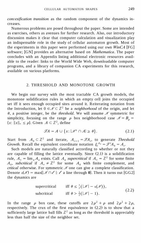
Ž . � < < 4 w xDenote i NN s max NN l ll : ll a line through 0 . Then it turns out GG2the dynamics are
1 < <supercritical iff u F NN y i NN ,Ž .Ž .22.2Ž .1 < <subcritical iff u ) NN y 1 .Ž .2
In the range r box case, these cutoffs are 2 r 2 q r and 2 r 2 q 2 r,Ž .respectively. The crux of the first equivalence in 2.2 is to show that a
sufficiently large lattice ball fills Z2 as long as the threshold is appreciablyless than half the size of the neighbor set.

GRAVNER AND GRIFFEATH250
To motivate the discussion of asymptotic shape for Threshold Growth,consider our
Basic Example: NN s B , u s 3.1
Note that this is the Moore neighborhood rule with highest supercriticalthreshold. From a suitably large seed A , say any configuration containing03 cells in a row, A rapidly forms a linearly expanding ‘‘lattice octagon,’’ sotŽ .1.4 holds with L s OO, the octagonal region bounded by vertices
1 1 1 1Ž . Ž . Ž ." , 0 , 0, " , " , " . The most straightforward route to Theorem 12 2 3 3
for specific rules is to compute iterates exactly. In our case, starting from�5 5 4the range 1 diamond seed D s x F 1 , it turns out that11
t < < < < < < < <TT D s x , x : max x q 2 x , 2 x q x F t q 2 . 2.3� 4Ž . Ž .1 1 2 1 2 1 2
Figure 1a shows each six updates in a new shade of gray. One can verifyŽ .2.3 by induction, checking the first few iterates directly and then observ-ing that the ‘‘sides’’ of the lattice octagons advance like boundaries ofhalf-spaces:
� 4 � 4x q 2 x F t ª x q 2 x F t q 1 ,1 2 1 2
Ž .whereas the ‘‘corners’’ advance with period 2 horizontal, vertical and 3Ž . Ž .diagonal; see Fig. 1b . Convergence to OO follows immediately from 2.3 .Next, given any finite A for which A s Z2, choose n so that D ; TT nA0 ` 1 0
n Ž . t tqn tq2 nand A ; TT D . Monotonicity 1.3 yields TT D ; TT A ; TT D , so0 1 1 0 1Ž .1.4 holds with L s OO, establishing Theorem 1 for our Basic Example.
Ž . 6 n Ž .FIG. 1. a TT DD; n s 1, . . . , 12; b detail of a stable corner.

CELLULAR AUTOMATON SHAPES 251
With larger neighborhoods and thresholds exact recursion becomesincreasingly difficult, so an alternate method is needed in order to estab-lish the Shape Theorem for Threshold Growth in full generality. An
w xapproach familiar to statistical physicists DKS, KrSp is based on half-spacepropagation. Roughly, the idea is that any expanding droplet should be-come locally flat as it grows, and so its displacement in direction a is
y � 4determined by the advance of a half-space H s x ? u F 0 , where u isuthe outward normal unit vector to the boundary of A in direction a .t
w xAfter some convex analysis GG1 , the recipe is essentially as follows. ByŽ y. y Ž . Ž .translation invariance, TT H s H q w u u for some function w uu u
known as the speed. From this computable data, form the region of R2
with extent wy1,
K s K s 0, 1rw u u.Ž .D1r wu
Then the asymptotic shape L is given by the polar transform of K,
L s K* s x : x ? y F 1 for every y g K . 2.4� 4 Ž .1r w
Let us see how the formalism works for our Basic Example. In this caseŽ . Ž . Ž .it turns out that K is a nonconvex 16-gon Fig. 2 , with vertices 1, 0 , 2, 1 ,
Ž .1, 1 , and 13 more dictated by the symmetries of the lattice. For instance,the diagram reflects the fact that while horizontal and vertical half-spacesadvance with speed 1, a half-space with slope 2 only advances at speed
' Ž1r 5 . Despite the nonconvexity, one gets K* s OO the small dark oc-.tagon in Fig. 2 , which we have already shown to be the asymptotic shape
Ž .L. For polygonal K one can obtain the shape but not the size of Lgeometrically by forming the intersection of half-spaces containing theorigin and normal to vectors ¨ which end at a vertex of the convex hull of
Ž .K. This intersection is the white octagon in Fig. 1. Since the limit set 2.4can also be represented as
L s w u u q Hy ,Ž .Ž .F uu
the size is then determined by a half-space velocity corresponding to oneof the polygonal sides.
Ž .Evidently 2.4 is valid for our Basic Example even though the boundaryof OO is not smooth so that the heuristics leading to the polar representa-
Ž .tion break down. In fact, formula 2.4 is always valid for ThresholdGrowth, and establishes Theorem 1 in full generality. A careful analysis
2relies on conjugate dynamics TT on R , needed to define w properly, suchthat
2 2TT A l Z s TT A l Z .Ž . Ž .

GRAVNER AND GRIFFEATH252
FIG. 2. K for range 1 box, u s 3.
With this trick one can mimic the technology of Euclidean Thresholdw x w xGrowth; GG1 and GG2 provide the details, including an argument that
w xL is always a polygon. See Wil1 for another proof of Theorem 1.Ž .According to 2.2 , there are 10 supercritical polygonal limit shapes for
w xNN s B , corresponding to thresholds 1, . . . , 10. Figure 2 of GG2 shows2them all as overlays when the successive dynamics are run from a suitablesmall initial seed. Clearly, smaller polygons correspond to larger thresh-olds, but the number of sides varies irregularly: 4, 8, 8, 12, 8, 12, 4, 4, 8, 8.Curiously, the limits L are identical for u s 7 and u s 8. As r, u ª `, in
2 w xsuch a way that urr ª l g 0, 2 , the limit shape L for NN andr, u r
threshold u converges to a convex L with piecewise smooth boundaryl
w x Ž .which is described in GG1 . In spite of formula 2.4 , we do not know howthe number of polygonal sides grows with r. Thus, we pose
Problem 1. As r ª `, determine the asymptotic growth rate for themaximal number of sides of L ; 1 F u F 2 r 2 q r.r, u
Another approach to asymptotic shape for monotone dynamics exploitssubadditi ity: the fact that growth accelerates as additional sites becomeoccupied. More precisely, for any initial seed A which fills Z2 eventually,0
Ž .and any site x, let t x denote the time until j occupies x starting fromtA . Suppose that once a sufficiently distant x is occupied, it must be the0

CELLULAR AUTOMATON SHAPES 253
case that x q A is totally covered after r additional updates, where r is0independent of x. Then, for any x, y g Z2,
t x q y F t x q t y q r , 2.5Ž . Ž . Ž . Ž .
Ž . Ž .since by 1.3 it can take no longer than t y additional updates for theŽ .configuration covering x q A at time t x q r to reach site x q y.0
Extend t to all of R2 by identifying each site of the lattice with the unitcell centered at that site, adopting some convention along cell edges. SetŽ . y1 Ž . 2 Ž . y1 Ž . Ž .¨ x s inf n t nx , x g R . It follows from 2.5 that n t nx ª ¨ xn
Ž . Ž .as n ª `, that ¨ x defines a norm, and that 1.4 holds with the convexlimit shape given implicitly as the unit ball
L s x : ¨ x F 1 . 2.6� 4Ž . Ž .
One uses monotonicity to show uniqueness of the limit starting fromsufficiently large seeds, just as in our recursive proof of Theorem 1 for theBasic Example. This line of argument was first applied about 25 years ago
w xin the context of random spatial interactions by Richardson Ric ; Section7 will discuss the method in more detail. Note, however, that the subaddi-tivity approach does not show that L is a polygon, nor does it give anygeometric information other than convexity and lattice symmetry.
For now, let us discuss the method’s applicability to Threshold Growthmodels, in which case we need only manufacture a suitable A and r0
Ž .leading to 2.5 . For our Basic Example it turns out that one can takeŽ .A s B and r s 4 as long as x f B , so 1.4 follows. To see this, first0 1 2
observe that the crystal started from B covers B after two updates. By1 2monotonicity, A covers B , and hence the process fills Z2. We formalize2 t tthe choice of r as a lemma, since it will be used again in Section 7 for anextension to random dynamics.
LEMMA. Let x g A be any site separated from A by ll `-distance at leastt 02. Restrict the occupied set and the dynamics to x q B from time t on. Such2dynamics will co¨er NN x at time t q 4.
Proof. Clearly A must contain three neighbors of x. Unless thosety1three occupied sites comprise a corner cell and its two adjacent neighborsŽ .other than x , it is straightforward to check that A covers x q Btq3 1using only the dynamics restricted to that neighborhood. If the three siteslie in a corner, and x f A , then some neighbor of one of the three sites1Ž .other than x must have been occupied at time t y 2. In this case onecan check that A covers NN x using only the dynamics restricted totq4x q B .2

GRAVNER AND GRIFFEATH254
Of course, carrying out such explicit case checking for larger ranges andthresholds rapidly becomes unmanageable, even with the aid of a com-puter. In order to describe the subadditivity approach to general supercrit-ical Threshold Growth, we digress briefly and consider some delicatecombinatorial questions connected with nucleation: Which A manage to0grow, and what is the mechanism for initial stages of growth? Here andthroughout the remainder of the paper, we say
< <A generates persistent growth if A ª ` as t ª `,0 t
and call the dynamics omni orous if, for every A which generates persis-0tent growth, A Z2. T. Bohman has recently provedt
w xTHEOREM 2 Boh . Threshold Growth with neighborhood B is omni o-r
Ž .rous for any supercritical u .
Bohman’s proof uses clever ‘‘energy’’ estimates, taking about two journal2 Ž .pages for the case u F r , and much longer for general u F r 2 r q 1 .
The latter part of his analysis depends on the geometry of squares, so it isunclear to which other neighborhoods the result generalizes. At least ifNN s B , the details of the construction also show that for any A whichr 0generates persistent growth, for any s - `, and x large, there is an
Ž .r s r r, u , s such that
x q B ; A ,s t Ž x .qr
Ž . Ž .which suffices to prove 1.4 by subadditivity, with L as in 2.6 . Note thatTheorem 2 also strengthens Theorem 1, implying that growth started fromany finite seed either stops eventually or attains asymptotic shape L.
A simple observation extends Theorem 1 to any monotone growthmodel on B parameterized by survival and birth thresholds u F u , withr 1 0L s L , the corresponding Threshold Growth shape. Namely, choose ar, u 0
Žlarge A so that each of its sites x sees at least u occupied sites i.e.,0< x < .B l A G u . For instance, a large lattice ball has this property as longr 0
Ž .as B , u is supercritical. Then at time 1, starting from A, all occupiedr 0sites survive since u F u , and all newly born sites see at least u1 0 0occupied sites by definition of the dynamics. In particular, the new config-
Ž .uration agrees with that of B , u Threshold Growth after one updater 0started from A. Iterating, we see that the dynamics agree with ThresholdGrowth at all times, so the asymptotic shape is the same. By monotonicity,the Shape Theorem holds for any larger seed.
We conjecture that any box neighborhood monotone rule, started fromany finite seed, either fixates or eventually fills Z2. However, the extensionof Bohman’s result is not immediate, so such rules might conceivably beable to fill in a periodic or an irregular infinite subset of the lattice.

CELLULAR AUTOMATON SHAPES 255
Ž .Problem 2. Let A be a monotone growth model with Moore or Bt r
neighborhood. Are periodic finite configurations possible? If the processgenerates persistent growth, must it be omnivorous?
By contrast, even the simplest nonmonotone rules can exhibit surprisingw xbehavior. Our next problem, which requires WinCA FG , or similar CA
software, drives home this point.
Problem 3. Consider the Biased Voter Automaton on NN s B , with2u s 6, u s 26. Thus, a cell becomes occupied if at least 6 of its 25 range0 1box neighbors are previously occupied, whereas occupied cells automati-
Žcally become empty. Thus, the birth and survival maps b and s are both.nondecreasing. Investigate this model’s crystal growth starting from the
�5 5 4seeds D ; B , where D denotes the 6-diamond y F 6 and B is the16 6 6 66-box.
Before continuing with the central theme of shape theory in the nextsection, we mention some additional nucleation problems about the very
Ž .smallest seeds which grow. Let g s g NN, u be the minimal number ofŽ .sites needed for persistent growth, and let n s n NN, u be the number of
seeds of size g which generate persistent growth and have their leftmostlowest sites at the origin. Parameters g and n play key roles in the First
w xPassage and Poisson]Voronoi Tiling results we have obtained in GG2w x Ž .and GG3 . For small neighborhoods box or not , one can determine g
and explicitly enumerate the n minimal droplets with a computer. ForŽ . Ž .instance, g B , 5 s 5 and n B , 5 s 574,718. As a little puzzle, the3 3
Ž . Ž .reader might check that in the threshold 2 case g B , 2 s 2 and n B , 2r r
Ž .s 4r 2 r q 1 . For larger u no such explicit evaluation of n is available forw xgeneral r ; a table of small cases appears in GG2 .
If u is small, then there are nucleating occupied sets of u cells, thesmallest possible size. For instance, if u F r 2, then any size u subset of ar = r box fills that box in one update, and thereafter covers a box of sider q t y 1 at each time t. The smallest example with g ) u is range 2,threshold 10, in which case B does not generate persistent growth, so2g ) u . However the 11 site configuration in Fig. 3 does nucleate, showingthat g s 11 in this case. The starting point in understanding g for large
Ž .neighborhoods is to demonstrate, for almost every l g 0, 2 , existence ofthe threshold-range limit
g B , lr 2Ž .r Elim s g l .Ž .2rrª`
When l is small the ‘‘design principles’’ of minimal nucleating droplets areeffectively random, but for large l they become severely constrained. Of

GRAVNER AND GRIFFEATH256
FIG. 3. A seed that grows for NN s B , u s 11.2
EŽ .particular interest is the largest l for which g l is as small as possible
g E s sup l: g E l s l .� 4Ž .c
Using interactive visualization to create large-range minimal droplets ofw xsize u , as well as related constructions, it is proved in GG4 that 1.61 -
g E - 1.66. Figure 4 shows level sets of the droplet which yields the lowercŽ .bound}a range 150 seed consisting of 36,760 cells white which grows for
u s 36,760. We know of no seed with 36,761 cells that grows for u s 36,761.
3. SOME SIMPLE NONMONOTONE RULES
As we will see shortly, more exotic crystals grow from cellular automa-Ž .ton rules without monotonicity property 1.3 . Typically, such rules give
rise to chaotic or pseudo-random structure so complicated as to defy
FIG. 4. A barely supercritical droplet for range 150 box, u s 36,760.
CELLULAR AUTOMATON SHAPES 257
mathematical analysis. In rare instances, however, starting from carefullychosen seeds, nonmonotone CA dynamics generate a periodic pattern inspace and time which can be spotted by computer visualization and thenchecked recursively. In this and subsequent sections we present a series ofsuch exactly solvable ‘‘counterexamples’’ in order to show that all the
Ž .Ž . Ž .regularity properties 1.5 i ] v of Threshold Growth shape theory mayfail in general.
Let us begin with a formalism which may be used to check that a givenCA evolves in a prescribed manner. The notation is somewhat burden-some, so we will first describe a simpler setup for solidification rules, thenproceed to the general framework.
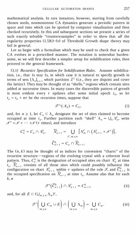
Ž .3.1 Recursi e Specification for Solidification Rules. Assume solidifica-tion, i.e., that 1s stay 1s, in which case it is natural to specify growth in
� 4 2 Žterms of sets L which partition Z i.e., they are disjoint and covern nG1.the lattice . They may be thought of as ‘‘shells,’’ regions which contain sites
added at successive times. In many cases the discernible pattern of growthis most evident every t updates after some initial epoch t , so let0t s t q nt be the recursion times, suppose thatn 0
TT t0 A s C , iŽ . Ž .0 0
and, for n G 1, let C ; L designate the set of sites claimed to becomen noccupied at time t . Further partition each ‘‘shell’’ L s D Lk , writen n k n
t Ž .NN s NN q ??? qNN t times , and introduce
k k k ll k tC s C l L , L s L l L q NN ,Ž .Dn n n nq1 m nq1ll , mFn
k kC s C l L .nq1 n nq1
Ž .The n, k may be thought of as indices for convenient ‘‘charts’’ of therecursive structure}regions of the evolving crystal with a coherent localpattern. Thus, C k is the designation of occupied sites on chart Lk at timen n
kt . L consists of all those sites which could possibly influence then nq1k kconfiguration on chart L within t updates of the rule TT, and C isnq1 nq1
kthe occupied specification on L at time t . Assume also that for eachnq1 nk, n
t k k kTT C l L s C , iiŽ .Ž .nq1 nq1 nq1
Ž .cand, for all E ; D L ,mF n m
TT t C j E l L s C . iiiŽ .D D Dm m mž / ž /mFn mFn mFn

GRAVNER AND GRIFFEATH258
Ž .Condition ii says that the configuration at time t restricted to a suitablenneighborhood of each chart for time t maps to the specified configura-nq1
Ž .tion on that chart after t updates. Condition iii ensures that once theconfiguration on the first n shells is known to be D C at time t , thenmF n m nno additional set of occupied sites E added at some later time can possiblychange the crystal on those shells. Consequently, a straightforward induc-
Ž . Ž .tion using i ] iii shows that
A s C for all n ,Dt mn
mFn
i.e., the true dynamics of the solidification model agrees with its a priorispecification.
Let us illustrate this formalism by sketching a few more details of theŽ . 2 Žproof of 2.3 for our Basic Example. There the iterates fill Z i.e., there
.are no permanently vacant sites , so it is natural to choose L s C , inn nŽ .which case solidification guarantees condition iii . As previously noted,
the shapes of the corners have periods 2 and 3, so it is perhaps simplest totake t s 6, and for sufficient ‘‘elbow room’’ t s 48, say. Then, in light of0Ž .2.3 , for n G 1 we can prescribe
L s Cn n
< < < < < < < <s x , x : 6n q 45 F max x q 2 x , 2 x q x F 6n q 50 ,� 4Ž .1 2 1 2 1 2
Ž . 48Ž . � w < < < < < <checking directly by computer! that TT D s max x q 2 x , 2 x q1 1 2 1< <x 4 kx F 50 . Next, we partition each shell L into suitable charts L which2 n ncorrespond to the sides and corners of the growing octagon. Let the eightcorner charts consist of those sites in L which are at most ll -distance 6n `
from each of the coordinate axes and lines x s "x . Let the eight side2 1charts be the connected components of the complementary portion of L .nThis decomposition and symmetry effectively reduces the verification of
Ž .condition ii for recursive specification to three cases: sides, and horizon-tal and diagonal corners. By construction, each chart Lk extends in anq1homogeneous fashion, meaning that the side charts extend consistentlywith lattice half-spaces while the corners extend consistently with lattice
Ž .wedges i.e., intersections of two half-spaces . Thus it suffices to check thatthe half space x q 2 x F n advances to x q 2 x F n q 1 in one update,1 2 1 2which is immediate from the threshold 3 update rule, and to verify that the
Ž .corner charts advance in keeping with 2.3 , each with the same profileafter six updates. For the diagonal corners this last is ensured by Fig. 1. Asimilar but simpler calculation handles the other corners and completesthe verification.

CELLULAR AUTOMATON SHAPES 259
The previous paragraph captures the spirit of our inductive scheme: bydecomposing a configuration into homogeneous charts one need onlycheck the claimed behavior of the update rule in a relatively small numberof cases rather than at every individual site. In practice, though, symbolicspecification is tedious and unenlightening. With effective CA visualiza-tion, it is often possible to check directly from a picture or animation thatthe evolution is recursively specified. For the remainder of the paper wewill present our exactly solvable examples via graphics which we hope thereader will find convincing. Use of a friendly interactive CA interface such
w xas WinCA FG greatly eases the verification.
A Biased Voter Example
As our first example of nonmonotone growth, we choose a Biased VoterCA with u - u . Namely, let us consider the range 2 box model with0 1
Žu s 1, u s 16, starting from a lattice ball of ‘‘radius’’ 7 about the0 1smallest size which gives rise to the interesting behavior we want to
.discuss . Throughout this paper, in keeping with WinCA, the lattice ball of1�5 5 4‘‘radius’’ r is taken to be x - r q . Figure 5 shows the configuration2 2
at time 40, suggesting that successive updates fill the plane in a predictablefashion. The totally occupied nonconvex star grows linearly, with a charac-teristic shape and periodic corners. Alternating occupied and vacant stripesof constant width 2 fill out the box which circumscribes the star. Eachupdate flips the states on the interior of the striped region, and a new
FIG. 5. Discontinuous density in the range 2 box Biased Voter Automaton, u s 1,0u s 16.1

GRAVNER AND GRIFFEATH260
outer occupied ring is added. By carefully eyeballing a few iterates with aprogram such as WinCA, it is easy to see that the dynamics reproduceexactly.
However, this is not a solidification model, so one needs to generalizeŽ .3.1 . The shells of the simpler scheme must be replaced by arbitraryconfigurations of the entire lattice, since sites may change state repeatedly.Thus, we partition all of Z2 into charts Lk at each time n. In place ofn
Ž .condition iii , the more extensive charts must be checked, but otherwisethe formalism is the same. Equivalently, one may frame the general case in
w xterms of CA solidification in three-dimensional space]time. See Toomfor examples of that approach.
Ž .3.2 Recursi e Specification for General Cellular Automata. t G 1 is the� k 4period of recursion; t s t q nt are the recursion times. L s L is an 0 n n
partition of Z2 for each fixed n. C designates the sites which are claimednŽ .to be occupied at time t . With the same notation as in 3.1 , assume thatn
Ž . Ž . Ž .3.1 i ] ii hold. Then A s C for all n.t nn
After a suitable initial time t during which the pattern stabilizes and0Ž .attains a sufficiently large size, application of 3.2 to our Biased Voter
example involves charts of seven varieties, in order to handle the interiorof the star, the exterior of the box, the interior of the edges of the star, theinterior of the edges of the box, the interior of the striped region, thecorners of the starrbox, and the concave corners of the star. All of thesepropagate with period 1 or 2, except for the last kind, which has period 4.Thus, simple recursive growth is easily verified by computer visualization.So what is the asymptotic shape L here? Note that the Hausdorff metric inŽ .1.4 does not distinguish between solid coverage and local occupancy witha uniformly positive density. Hence L agrees with the normalized ‘‘lightcone,’’ a Euclidean box BB of side 4, centered at the origin, which4represents the largest possible region attainable by range 2 growth. Inmodels which do not fill the lattice completely as they spread, a moredetailed asymptotic density profile is clearly desirable in order to capturesubtler aspects of crystal geometry such as that indicated in Fig. 5.
To this end, introduce the measure m concentrated on A rt, andt tassigning mass 1rt 2 to each point in the normalized configuration. Let mbe a measure on R2 with compact support. Then we say that ty1A ª m intmeasure as t ª ` if m converges weakly to m, that is to say,t
f dm ª f dm for all f g CC R2 . 3.3Ž . Ž .H Ht c

CELLULAR AUTOMATON SHAPES 261
Note that, since the m are uniformly bounded and have uniformly boundedtsupport, they have at least one limit point. As we shall see, the number oflimit points may be uncountable. We should also observe that while thisnotion can capture densities other than 1, it also sometimes loses informa-tion. For instance, if ty1A converges to a line segment in the Hausdorfftmetric, then ty1A converges to 0 in measure. One general remark is alsotin order. Namely, suppose m is any limit point of m . Since A ; Z2 andt tZ2rt converges to Lebesgue measure in the above sense, it follows thatŽ . Ž . 2m K F area K for any measurable K ; R . Hence there is a measurable
2 w xf : R ª 0, 1 such that m s f dx. In this sense, we could simply writety1A ª f.t
For our Biased Voter example, let SS denote the Euclidean star polygonŽ . Ž .with four vertices at 0, "1 and "1, 0 , and four vertices at the corners
of BB . Then A rt converges in measure to the m which has density 1 on4 t1
SS , on BB _ SS , and 0 elsewhere. Even for growth models which do not fill42
the lattice, the most common scenario would seem to be an asymptoticŽ . Ž .shape with constant local density throughout, i.e., m dx s c ? 1 x dx forL
some c ) 0. Another plausible behavior is a smooth ‘‘hydrodynamic’’profile over the support of L. A novel feature in the present case is theabrupt change of density at the boundary of SS . Additional instances ofŽ .3.3 will appear throughout the paper.
Figure 5 also suggests a complex phase portrait for nonmonotone BiasedVoter automata as the thresholds u , u vary, with solid growth for some0 1choices, spreading rings in others, and mixed profiles for an intermediateregime. Indeed, some initial experimentation strongly suggests the exis-tence of several phase transitions. Moreover, these systems are sufficientlysimple, and closely related to Threshold Growth, that a rather completeunderstanding of their shape theory should be possible.
Problem 4. Let A be a Biased Voter automaton with range r boxtneighborhood, birth threshold u , and survival threshold u . Assume that0 1u - u and u F 2 r 2 q r. Determine the dependence of the model’s0 1 0crystal growth on r, u , u , and the size and geometry of the initial0 1seed A .0
For the remainder of our study of deterministic growth we will restrictattention to totalistic Moore neighborhood models, focusing on the sim-plest nonlinear dynamics which exhibit complexity of various kinds. Anespecially fascinating class are the Exactly u solidification rules in which avacant site becomes permanently occupied if exactly u of its eight neigh-bors are occupied. Only the cases u s 1, 2, 3 are capable of persistentgrowth from finite seeds, by comparison with u s 4 Threshold Growth,which is convex-confined. Let us first consider the case u s 1.

GRAVNER AND GRIFFEATH262
Exactly 1 Solidification
We will study the evolution starting from a single occupied cell at theorigin in considerable detail. A key initial observation is that the locationsŽ ."t, " t join the crystal at time t: the occupied set grows along the
'diagonals at the fastest possible speed, c s 2 . This follows from the fact� 4 �5 5that, as in any Moore neighborhood CA started from 0 , A ; B s x `t t
4F t , so by induction, at time t q 1 each corner cell of B _ B sees onlytq1 tthe diagonal cell that was added at time t. In general, by a ladder we meanany local CA configuration which propagates over time in some directionu, periodically in space. A c-ladder is a ladder which propagates with the
Ž .fastest velocity allowed by NN the ‘‘speed of light’’ . In the present case, thefour diagonal trails are c-ladders one cell wide and with spatial period 1.We will encounter more elaborate ladders later in the paper. For now,note that the Exactly 1 rule grows persistently from any finite A since0there must be extremal occupied cells in the diagonal directions which giverise to permanent c-ladders.
� 4Starting from 0 , the intricate growth of A off the diagonals is showntin Fig. 6 at t s 55. One immediately notices the recurring lacelike motifs,in striking contrast to any of the crystals discussed so far. More carefulscrutiny reveals an exactly recursive structure along dyadic sequencest s 2 n, which permits us to describe the occupied set at arbitrary times innterms of the binary expansion of t. This representation, in turn, lets us
FIG. 6. The Exactly 1 solidification rule, started from a singleton, after 55 updates.

CELLULAR AUTOMATON SHAPES 263
compute the asymptotic density with which the Exactly 1 rule fills Z2,subsequential limit shapes L along subsequences t s r2 n, and boundaryr nlengths of the L . The same phenomenology is observed in many otherrintractable CA rules, so it is satisfying to quantify a ‘‘regular fractal
w xpattern’’ TM, p. 39 which serves as an exactly solvable prototype for whatw xPackard and Wolfram PW called growth with ‘‘corrugated boundaries.’’
Details follow.Before proceeding, though, we pause to contrast the behavior of the
most familiar and exactly solvable totalistic CA on B which generates a1fractal: XOR over the Moore neighborhood. Starting from a singleton, thatmodel generates a space]time pattern which is a slightly more complicatedthree-dimensional counterpart to the Sierpinski lattice obtained fromPascal’s Triangle Modulo 2. In the same way that row 2 n y 1 of Pascal’sTriangle has all odd coefficients and row 2 n has only two, XOR on B fills1each quadrant of B n with a regular array of 2 = 2 occupied boxes2surrounded by empty frames of width 1 at time 2 n y 1, and then collapsesto only nine occupied sites at time 2 n. Evidently this process does not growpersistently, although it does have a disconnected limit shape L alongr
n Ž .each subsequence t s r2 for fixed r g 0, 1 . These shapes are cross-sec-nw xtions through a 3D fractal; almost all have density 0. See Wil2 for an
early account of the fractal structure of linear cellular automata. LinearityŽ .property 1.2a makes the analysis easy in comparison with Exactly 1, to
which we now return.
The Exactly 1 Recursion
Let A be the occupied set at time t for the Exactly 1 rule started fromt� 4 nA s 0 . At times t s 2 , n G 3, we claim that the crystal has the0 n
� 4 Žfollowing properties in the octant 0 F x F x with analogous structure2 1.over the rest of the lattice, by symmetry :
Ž . n Ž n n.i The only occupied site with x G 2 is 2 , 2 . All other sites of1Ž n .the form 2 , x are vacant, with at least two occupied neighbors of the2
Ž n .form 2 y 1, y , and so never join the crystal.Ž .ii The only occupied site with x s 0 is the origin, and the2
occupied sites with x s 1 have first coordinates 1, 3, 7, . . . , 2 n y 1.2
Ž . Ž ny1 ny1.iii The configuration on the lattice region bounded by 2 , 2 ,Ž n ny1. Ž n n .2 y 1, 2 , and 2 y 1, 2 y 1 is an exact translate of the config-
Ž . Ž ny1 . Ž ny1uration on the region bounded by 0, 0 , 2 y 1, 0 , and 2 y 1,ny1 . Ž ny1 ny1.2 y 1 . The configuration on the region bounded by 2 , 2 ,
Ž n ny1. Ž n .2 y 1, 2 , and 2 y 1, 1 is the mirror reflection of the same pat-Ž ny1 .tern. Finally, the configuration on the region bounded by 2 q 1, 2 ,
Ž n . Ž ny1 ny1 .2 y 2, 2 , and 2 q 1, 2 y 1 is an exact rotated translate of the

GRAVNER AND GRIFFEATH264
Ž . Ž ny1 . Ž ny1configuration on the region bounded by 2, 2 , 2, 2 y 1 , and 2 yny1 . � ny14 w ny1 x1, 2 y 1 , and all sites in lattice intervals 2 = 2, 2 y 1 ,
w ny1 n x � 4 w ny1 n x � 42 , 2 y 1 = 0 , and 2 , 2 y 2 = 1 are vacant.Ž .Figure 7 shows the configurations on the octant at time 8 n s 3 and
Ž . Ž . Ž .time 32 n s 5 . Properties i ] iii may be verified at time 8 by inspection,and at subsequent times t s 2 n by induction. Assuming the hypothesis forn
Ž n n.n, the key observations are that c-ladders emanate from 2 , 2 , oneproceeding along the diagonal x s x , and one heading ‘‘southeast’’ along2 1
Ž n. nx s yx , and that by symmetry all sites of the form x , 2 with 2 q2 1 1nq1 Ž n2 F x F 2 y 1 are vacant after time 2 q 1 any such site which is2
unoccupied must have an even number of occupied neighbors, and so.cannot join the crystal . Thus further growth within the octant is divided
Ž .into three triangular regions, as in iii but with n replaced by n q 1,which evolve independently with mixed ‘‘all 1’’ and ‘‘all 0’’ boundaryconditions. The first two new regions exactly replicate the conditions of theoctant up to time 2 n y 1, and so generate the same structure as claimed.The final triangular region also replicates this structure after a slightdisplacement. The c-ladder along its upper edge proceeds southeast until
Ž nq1 . Ž .it occupies the point 2 y 1, 1 , as desired in part ii of the induction.We omit further details, which are checked in a similar fashion.
E¨aluation of the Density
< < < � 4 <n nWrite a s A and b s A l x G 0, 0 F x F x . Note firstn 2 y1 n 2 y1 1 2 1that, dividing the lattice into octants and appealing to symmetry, a snŽ n . Ž n .8 b y 2 y 1 q 4 2 y 2 q 9 for n G 1. Here the first term countsn
FIG. 7. One octant of Exactly 1 solidification, started from a singleton, after 8 and 32updates.

CELLULAR AUTOMATON SHAPES 265
occupied sites not on the diagonals x s "x and outside B , the second2 1 1term counts occupied sites on the diagonals and outside B , and the third1term counts occupied sites inside B . Thus,1
a s 8b y 4 ? 2 n y 7.n n
Ž .Next, denote the triangular regions shown in the right half of Fig. 7,counterclockwise from the bottom left, by I, II, III, and IV. Then the four
Ž . Ž .contributions to b have cardinality b I and IV , b y 2 III , andnq1 n nŽ n . Ž .b y 2 y 2 y n y 2 II . For the last formula note that, as mentionedn
earlier, if one cuts from I the diagonal, and the sites with x s 1, and the2sites with x s 0, then the remainder is isomorphic to II. Therefore,2
b s 4b y 2 n y n y 2,nq1 n
and so
a s 8 4b y 2 n y n y 2 y 4 ? 2 nq1 y 7Ž .nq1 n
s 4 8b y 4 ? 2 n y 7 q 16 ? 2 n q 28 y 8 ? 2 nŽ .n
y 8n y 16 y 4 ? 2 nq1 y 7s 4a y 8n q 5.n
The solution is
4nq2 q 24n y 7a s .n 9
4< <nIn particular we see that a r B ª , the asymptotic density, and son 2 y1 94yn Ž . �5 5 4 Ž .n2 A ª 1 x dx, where L s BB s x F 1 , in the sense of 3.3 .`2 L 19
Let us pause here to pose four problems. The first two are exercises forthe enterprising reader. The third, motivated by empirical observation thatmany small seeds induce bounded perturbations of the singleton-seedrecursion, may well involve substantial effort. The fourth is quite likelymost difficult.
w xProblem 5. Packard and Wolfram PW observed similar behavior inŽthe Exactly 1 rule on the nearest neighbor diamond cf. rule 174, shown in
.their Fig. 2 , although they did not identify a recursive structure orcompute its asymptotic density. Mimic the derivation above to show that
2the density starting from a single occupied cell equals .3
Problem 6. Starting from a single occupied cell, compute the asymp-Žtotic density of the Exactly 1 Or At Least u solidification rule in which
Ž . .b i s 1 iff i s 1 or i G u for 2 F u F 8.

GRAVNER AND GRIFFEATH266
Problem 7. Does the Exactly 1 solidification rule on the Moore neigh-4borhood fill the plane with asymptotic density starting from any initial9
seed?
Ž .Problem 8. Find an elementary CA solidification or otherwise with acomputable asymptotic density which is irrational.
Subsequential Limit Shapes
Closer inspection of Exactly 1 recursive growth, driven by c-ladders,identifies asymptotic shapes L along all subsequences t s r2 n for fixedr nr. The limits are generated by a recursive scheme reminiscent of the von
w xKoch algorithm vK . To describe it, introduce the binary expansion` yk � 2 5 5 4r s Ý d 2 , k an integer, and d s 1. Write BB s x g R : x F s .`k k 0 k s0 0
Starting from BB yk , successively add three translates of BB yk for every02 2k ) k such that d s 1, at the ‘‘exposed’’ corners of each previous square.0 k
7Figure 6 is suggestive of the algorithm for r s 0.111 s . Note that8
smaller squares are added at each of four corners of the initial square, butonly three of four corners are exposed at later stages. L is the monotonerlimit when this recursion is carried out for all k G k . Note that L s 2 L ,0 2 r r
1w .so by normalizing suitably it suffices to consider r g , 1 . Now the same2
methods as for the case r s 1 can be used to show that lim ty1Anª` n tn4 Ž . Ž .y1s 1 x dx in general. Thus we have our first example where i ofr L9 rŽ . Ž .1.5 holds, but ii fails, with convergence to distinct limit shapes alongsuitable subsequences. All of these ‘‘corrugated’’ subsequential limits
Žexcept L s BB are nonconvex, and as we are about to see, many e.g.,1 1.L have genuinely fractal edges, i.e., boundary curves with self-similar6r7
pieces of dimension greater than 1.
Asymptotic Boundary Length
Let us conclude our discussion of the Exactly 1 rule by analyzing the1N yk w .lengths of its asymptotic boundaries. First suppose r s Ý d 2 g , 1 ,1 k 2
with d s 1, and write s s Ýk d . Then it is not hard to check byN k 1 lŽ .induction that the boundary length l r of L is given byr
N4 4 s ykkl r s 1 q d 3 2 .Ž . Ý k3 3
ks1
Hence, if r has a nonterminating binary expansion,
`4 4 s ykkl r s 1 q d 3 2 .Ž . Ý k3 3
ks1

CELLULAR AUTOMATON SHAPES 267
This asymptotic boundary length l, as a function of r, is lower semicontin-uous, sometimes finite and sometimes infinite, but not continuous at anyvalue where it is finite. Assuming that s rk ª s , the Hausdorff dimen-k
� Ž . Ž .4sion of the boundary of L is given by max 1, s ln 3 r ln 2 . Thus, therHausdorff dimension is not continuous anywhere: within any e-neighbor-
Žhood of any r there is an L with boundary of finite length dimension0 r1. Ž . Ž .1 , an L with boundary of the largest possible dimension ln 3 r ln 2 ,r2
and a limit shape with any intermediate dimension as well.
Exactly 2 Solidification
We conclude this section by turning to the Exactly u solidification rulewith u s 2. How does a crystal grow from small seeds when exactly two ofeight neighbors must be occupied for a vacant site to join? Now a singletonobviously does nothing, but observe that a 2 = 2 initial seed spreads in the
3 Žshape of a diamond, with density and speed 1 along the axes. The4. y1computation is quite doable with paper and pencil. Thus, t A ªt
3 2Ž . � 5 5 4 Ž .1 x dx, where DD s x g R : x F 1 , in the sense of 3.3 . The1DD4
evolution from this seed also reveals horizontal and vertical ladders ofwidth 2 along the diagonals of the diamond which suggest a simplesufficient condition for growth in terms of an ‘‘exposed’’ dyad. Namely,suppose that, after suitable translation and reflection through one or both
�Ž . Ž .4axes, A contains the dyad 0, 0 , 0, 1 and is otherwise confined to the0� 4half-space x - 0 . Then, in the new coordinate system, a straightforward1
� 4induction shows that A > 0 F x - t, x s 0 or 1 . On the other hand, itt 1 2� 2 5 5 4is easy to check that no diamond seed D s x g Z : x F n grows at1n
all, and that any n = n square seed with n G 3 stops after one step. Herewe encounter our first growth model in which certain seeds grow, whereasothers of arbitrarily large size do not, depending on the geometry. Is thereany hope for a coherent shape theory in such a situation?
w xOne approach, proposed by Packard and Wolfram PW , is to studygrowth from disorder, e.g., from random subsets of a box B . Many CALrules exhibit a characteristic, linearly spreading shape when started fromthe vast majority of such random finite configurations. The Exactly 2 rulewould seem to conform to this scenario, with limit DD, although the genericdynamics are sufficiently pseudo-random to offer little hope for rigorousresults. A succession of horizontal and vertical ladders typically emergefrom the edges of the crystal growth, the first such determining theextreme points of the limiting spreading diamond. Regions of regulargrowth with the pattern of the 2 = 2 seed may also be observed. Indeed,even n = 2 rectangles for any n / 2 exhibit essentially the same complex-
Ž .ity as random seeds apart from symmetry about the axes, of course .Figure 8 shows the evolution from a horizontal dyad at t s 100. Conceiv-

GRAVNER AND GRIFFEATH268
FIG. 8. Exactly 2 solidification, from a horizontal dyad, after 100 updates.
ably one could prove convergence to DD based on the regular emergence ofindestructible ladders at the boundary, but the prospect seems too dim topose this as an open problem.
4. LIFE WITHOUT DEATH
The Exactly 3 growth model is one of our favorites}able to generateremarkably complex crystals, yet amenable to some substantive experimen-tal mathematics. As noted in the Introduction, this is Conway’s Game ofLife with no 1 ª 0 transitions, so upon discovering its exotic properties a
Ž .few years ago we named it Life without Death LwoD, pronounced el ? wod .Not surprisingly, we have since learned that some of the extraordinary
w xbehavior of this model has also been noted by Stephen Wolfram Wol2and various members of the LifeList Internet forum devoted to Conway’srule. The earliest reference to LwoD in the literature would appear to bew xTM, pp. 6]7 .
Starting from most small seeds, e.g., from all lattice balls of ‘‘radius’’ upto 10, LwoD fixates. However, beginning with ‘‘radius’’ 11, as shown in Fig.9 at time 1250, many such lattice balls produce spreading crystals reminis-

CELLULAR AUTOMATON SHAPES 269
FIG. 9. Life without Death started from a lattice ball of ‘‘radius’’ 11: Insets at the upperleft and right show a ladder tip and a parasitic shoot, respectively.
cent of the ancient Zia design on the New Mexico state flag. To highlightstructural elements, we have drawn successive updates periodically using a256-color gray scale gradient. Evidently, LwoD growth is dominated by adendritic phase which we call la¨a, since its porous, seemingly organicform spreads slowly and unpredictably. Interspersed are horizontal andvertical ladders of a single design, which emerge seemingly at random from
1the lava, and advance at speed by a back-and-forth weaving motion of3
period 12 with four spatial phases at the tip. The upper left inset of Fig. 9magnifies one of the tips along the axes; of course the others are reflec-tions and rotations by symmetry. Ladders seem to outrun the surroundinglava, suggesting that the recursive structures along the axes should persistindefinitely. But after more than 1100 updates, ladders which emerged

GRAVNER AND GRIFFEATH270
from the lava collide with edges of the ladders along the axes, and parasiticshoots are formed. These structures, which can only evolve on the edges ofladders or other shoots, also emerge occasionally from the interstices
2between lava and ladders. Shoots have speed ; one is magnified in the3
upper right inset of Fig. 9. Thus the parasites race along the edges of theirhost ladders until they reach the tips, at which time any of several lavaeruptions takes place depending on the phase of the host]parasite interac-tion. Consequently, it is not at all clear whether LwoD started from the11-ball grows persistently or fixates.
There are only two scenarios for which we know how to answer thepersistence question. If the growth produces a fixed core surrounded by
Žfinitely many autonomous ladders extending away from the origin with no.active shoots! , then the growth persists, its asymptotic shape is the
degenerate cruciform
1 1< < < <CC s x F , x s 0 j x s 0, x F ,� 4 � 41 2 1 23 3
Ž . Ž . Ž . Ž .and we obtain an example where i and ii of 1.5 hold, but v fails. Onthe other hand, if all shoots and ladders are stopped by interference withlava, and later the slow dendritic growth also grinds to a halt, then thesystem has fixated. Various small seeds lead to each of these outcomes,sometimes after hundreds or even thousands of updates. Empirical evi-dence, and a seeming affinity with stochastic dynamics, suggest nucleation:once a sufficiently large boundary layer of lava has formed, it wouldappear increasingly unlikely for all growth to stop. Here are two illustrativecases which can be resolved.
Problem 9. Run Life without Death for 100 updates starting from the1�5 5 418-ball: x - 18 , and for 1000 updates starting from2 2
to decide whether or not these processes grow persistently.

CELLULAR AUTOMATON SHAPES 271
One can catalog all of the ‘‘elementary’’ interactions between pairs ofladders, and between shoots and ladders. For instance, synchronizedladders meeting at right angles can form a clean corner, ladders meetinghead-on can form a clean final border, and a ladder can be cleanly blockedby colliding at right angles with the side of another formed previously.Eruptions of lava, and shoot creation are also possible results, dependingon the relative phases. It is less clear whether one can describe succinctlythe preconditions for spontaneous emergence of shoots and ladders fromlava. Regardless, the resulting complex dynamics self-organize so that verylarge motifs appear again and again as the crystal evolves. A strikingexample of this propensity, starting from an 80-ball, is discussed in
w x Žan April 1995 recipe of Gri2 http:rrpsoup.math.wisc.edur archiver.recipe26.html . Over the first 10,000 updates a configuration of more than
250 = 250 cells, containing an empty region larger than 150 = 150, repli-cates several times in the diagonal direction before being disrupted by acircuitous chain of interactions. Such complex manifestations invoke suspi-cions of even more exotic, unseen possibilities. Are there supremelypowerful, but exceedingly rare, self-organizing LwoD structures? None hasbeen observed from simple seeds or random initial conditions, but Noam
Ž .Elkies private communication notes that there are c-ladder parasitescapable of propagating between parallel sets of shoots on ladders.
In light of the previous paragraph, our favorite open question concern-ing LwoD is a difficult one.
Problem 10. Find a finite A from which LwoD grows persistently and0fills Z2 with positive density.
Experiments from large lattice balls suggest that such seeds abound.However, the only solution we can imagine would entail construction of aladder gun, or some other space-filler analogous to those for Conway’sGame which will be discussed in Section 6. We think there is at least areasonable chance of such a recursive design, but its discovery wouldcertainly require great ingenuity.
As an illustration that the complexity of LwoD can, to some extent, becharacterized mathematically, we will now prove a result which captures itssensitive dependence on initial conditions.
THEOREM 3. Let A be Life without Death. Gi en any finite A , there aret 0configurations C and C , each consisting of 28 cells, such that A grows1 2 tpersistently from A j C , but fixates from A j C .0 1 0 2
ŽNote that the design and location of C and C are allowed to depend1 2.on A , but not their size.0

GRAVNER AND GRIFFEATH272
Proof of Theorem 3. The idea is to form a closed frame around A ,0from a minimal number of strategically placed occupied cells, so that thegrowth emanating from A is completely confined by the time it reaches0the frame. If the frame is static, then this should constrain growth to itsbounded interior, thereby ensuring fixation. If the frame instead producesisolated ladders traveling away from its exterior, then since the growth ofA is still controlled, persistent growth is guaranteed. Clearly, a closed0
Žll -circuit of occupied sites i.e., a loop of sites connected by N, S, E, and1.W transitions prevents any interaction between the dynamics on its
interior and those on its exterior. So our frame need only include such acircuit to achieve the desired containment.
The details of the construction are as follows. First, choose L so thatA ; B . Next, for a suitably large N, place a 4-cell side seed0 L
along the positive x axis so that the empty site between its top and1Ž .bottom cells is located at 4NL q 1, 0 , and a 3-cell corner seed
Žin the first quadrant so that its middle cell is located at 4NL y 18, 4NL y. Ž18 . Place three more such side seeds symmetrically along the axes with
.their isolated cells closest to the origin , and three more corner seedsŽsymmetrically along the diagonals of the other quadrants with their
.middle cells closest to the origin . The 28-cell collection of corner and sideseeds constitutes configuration C in the statement of the theorem.1Configuration C agrees with C , except that2 1
v the empty site between the top and bottom cells of the side seedŽ .along the positive x-axis is at 4NL, 0 ;
v the leftmost cell of this side seed is moved 9 sites further to the leftŽso that there are a total of 11 empty sites between it and the rightmost
.cell ;

CELLULAR AUTOMATON SHAPES 273
v the middle cell of the corner seed in the first quadrant is atŽ .4NL y 22, 4NL y 22 ; with symmetric changes to the other six seeds.
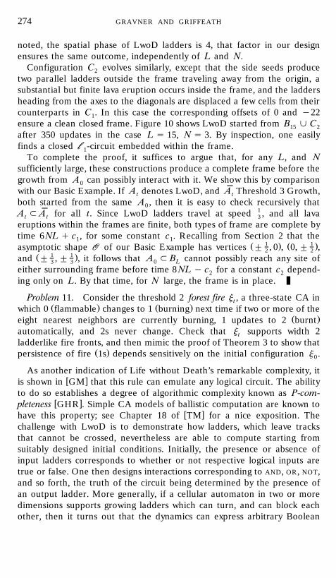
Easiest to check is the evolution of the side seed pictured above. With alittle care and patience, one can verify by hand that the result is twoladders, traveling north and south, cleanly fused along the axis. Thus, theside seeds of C spread away from the axes to begin forming a frame.1Simultaneously, as can only readily be checked with a computer, after asubstantial but finite eruption of lava, the corner seeds each produce apair of ladders heading from the diagonals toward the axes. The cornermotifs of Fig. 10 illustrate this effect. Moreover, the offsets of q1 andy18 from 4NL in our design ensure that the pairs of ladders headingtoward one another are aligned exactly, and their collisions produce aclean closed frame with no additional shoots or lava. Since, as previously
FIG. 10. Formation of a frame with exterior ladders from 28 cells: Here L s 15, N s 3,t s 350.
GRAVNER AND GRIFFEATH274
noted, the spatial phase of LwoD ladders is 4, that factor in our designensures the same outcome, independently of L and N.
Configuration C evolves similarly, except that the side seeds produce2two parallel ladders outside the frame traveling away from the origin, asubstantial but finite lava eruption occurs inside the frame, and the laddersheading from the axes to the diagonals are displaced a few cells from theircounterparts in C . In this case the corresponding offsets of 0 and y221ensure a clean closed frame. Figure 10 shows LwoD started from B j C15 2after 350 updates in the case L s 15, N s 3. By inspection, one easilyfinds a closed ll -circuit embedded within the frame.1
To complete the proof, it suffices to argue that, for any L, and Nsufficiently large, these constructions produce a complete frame before thegrowth from A can possibly interact with it. We show this by comparison0with our Basic Example. If A denotes LwoD, and A Threshold 3 Growth,t tboth started from the same A , then it is easy to check recursively that0
1A ; A for all t. Since LwoD ladders travel at speed , and all lavat t 3
eruptions within the frames are finite, both types of frame are complete bytime 6NL q c , for some constant c . Recalling from Section 2 that the1 1
1 1Ž . Ž .asymptotic shape OO of our Basic Example has vertices " , 0 , 0, " ,2 21 1Ž .and " , " , it follows that A ; B cannot possibly reach any site of0 L3 3
either surrounding frame before time 8 NL y c for a constant c depend-2 2ing only on L. By that time, for N large, the frame is in place.
Problem 11. Consider the threshold 2 forest fire j , a three-state CA intŽ . Ž .which 0 flammable changes to 1 burning next time if two or more of the
Ž .eight nearest neighbors are currently burning, 1 updates to 2 burntautomatically, and 2s never change. Check that j supports width 2tladderlike fire fronts, and then mimic the proof of Theorem 3 to show that
Ž .persistence of fire 1s depends sensitively on the initial configuration j .0
As another indication of Life without Death’s remarkable complexity, itw xis shown in GM that this rule can emulate any logical circuit. The ability
to do so establishes a degree of algorithmic complexity known as P-com-w xpleteness GHR . Simple CA models of ballistic computation are known to
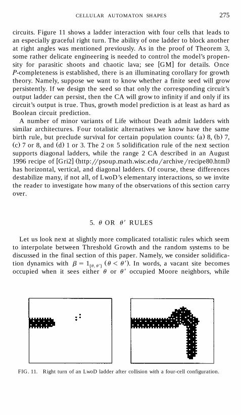
w xhave this property; see Chapter 18 of TM for a nice exposition. Thechallenge with LwoD is to demonstrate how ladders, which leave tracksthat cannot be crossed, nevertheless are able to compute starting fromsuitably designed initial conditions. Initially, the presence or absence ofinput ladders corresponds to whether or not respective logical inputs aretrue or false. One then designs interactions corresponding to AND, OR, NOT,and so forth, the truth of the circuit being determined by the presence ofan output ladder. More generally, if a cellular automaton in two or moredimensions supports growing ladders which can turn, and can block eachother, then it turns out that the dynamics can express arbitrary Boolean
CELLULAR AUTOMATON SHAPES 275
circuits. Figure 11 shows a ladder interaction with four cells that leads toan especially graceful right turn. The ability of one ladder to block anotherat right angles was mentioned previously. As in the proof of Theorem 3,some rather delicate engineering is needed to control the model’s propen-
w xsity for parasitic shoots and chaotic lava; see GM for details. OnceP-completeness is established, there is an illuminating corollary for growththeory. Namely, suppose we want to know whether a finite seed will growpersistently. If we design the seed so that only the corresponding circuit’soutput ladder can persist, then the CA will grow to infinity if and only if itscircuit’s output is true. Thus, growth model prediction is at least as hard asBoolean circuit prediction.
A number of minor variants of Life without Death admit ladders withsimilar architectures. Four totalistic alternatives we know have the same
Ž . Ž .birth rule, but preclude survival for certain population counts: a 8, b 7,Ž . Ž .c 7 or 8, and d 1 or 3. The 2 OR 5 solidification rule of the next sectionsupports diagonal ladders, while the range 2 CA described in an August
w x Ž .1996 recipe of Gri2 http:rrpsoup.math.wisc.edurarchiverrecipe80.htmlhas horizontal, vertical, and diagonal ladders. Of course, these differencesdestabilize many, if not all, of LwoD’s elementary interactions, so we invitethe reader to investigate how many of the observations of this section carryover.
5. u OR u 9 RULES
Let us look next at slightly more complicated totalistic rules which seemto interpolate between Threshold Growth and the random systems to bediscussed in the final section of this paper. Namely, we consider solidifica-
Ž .tion dynamics with b s 1 u - u 9 . In words, a vacant site becomes�u , u 94occupied when it sees either u or u 9 occupied Moore neighbors, while
FIG. 11. Right turn of an LwoD ladder after collision with a four-cell configuration.
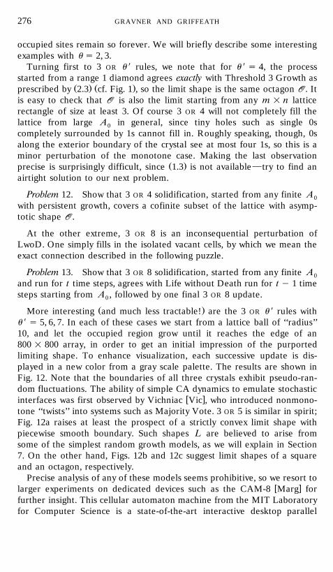
GRAVNER AND GRIFFEATH276
occupied sites remain so forever. We will briefly describe some interestingexamples with u s 2, 3.
Turning first to 3 OR u 9 rules, we note that for u 9 s 4, the processstarted from a range 1 diamond agrees exactly with Threshold 3 Growth as
Ž . Ž .prescribed by 2.3 cf. Fig. 1 , so the limit shape is the same octagon OO. Itis easy to check that OO is also the limit starting from any m = n latticerectangle of size at least 3. Of course 3 OR 4 will not completely fill thelattice from large A in general, since tiny holes such as single 0s0completely surrounded by 1s cannot fill in. Roughly speaking, though, 0salong the exterior boundary of the crystal see at most four 1s, so this is aminor perturbation of the monotone case. Making the last observation
Ž .precise is surprisingly difficult, since 1.3 is not available}try to find anairtight solution to our next problem.
Problem 12. Show that 3 OR 4 solidification, started from any finite A0with persistent growth, covers a cofinite subset of the lattice with asymp-totic shape OO.
At the other extreme, 3 OR 8 is an inconsequential perturbation ofLwoD. One simply fills in the isolated vacant cells, by which we mean theexact connection described in the following puzzle.
Problem 13. Show that 3 OR 8 solidification, started from any finite A0and run for t time steps, agrees with Life without Death run for t y 1 timesteps starting from A , followed by one final 3 OR 8 update.0
Ž .More interesting and much less tractable! are the 3 OR u 9 rules withu 9 s 5, 6, 7. In each of these cases we start from a lattice ball of ‘‘radius’’10, and let the occupied region grow until it reaches the edge of an800 = 800 array, in order to get an initial impression of the purportedlimiting shape. To enhance visualization, each successive update is dis-played in a new color from a gray scale palette. The results are shown inFig. 12. Note that the boundaries of all three crystals exhibit pseudo-ran-dom fluctuations. The ability of simple CA dynamics to emulate stochastic
w xinterfaces was first observed by Vichniac Vic , who introduced nonmono-tone ‘‘twists’’ into systems such as Majority Vote. 3 OR 5 is similar in spirit;Fig. 12a raises at least the prospect of a strictly convex limit shape withpiecewise smooth boundary. Such shapes L are believed to arise fromsome of the simplest random growth models, as we will explain in Section7. On the other hand, Figs. 12b and 12c suggest limit shapes of a squareand an octagon, respectively.
Precise analysis of any of these models seems prohibitive, so we resort tow xlarger experiments on dedicated devices such as the CAM-8 Marg for
further insight. This cellular automaton machine from the MIT Laboratoryfor Computer Science is a state-of-the-art interactive desktop parallel
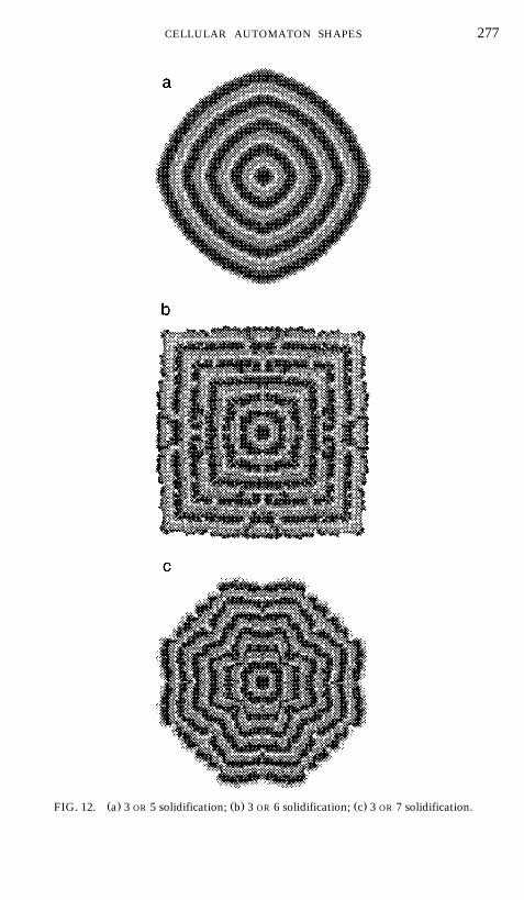
CELLULAR AUTOMATON SHAPES 277
Ž . Ž . Ž .FIG. 12. a 3 OR 5 solidification; b 3 OR 6 solidification; c 3 OR 7 solidification.

GRAVNER AND GRIFFEATH278
processor, offering a unique combination of computing power and visual-ization capability for the study of CA dynamics. To date, our mostinteresting CAM-8 discovery about 3 OR 6 growth is the emergence ofcertain structures, at the corners, with very large but finite period. Perhapsthese can be used to confirm a square limit L, at least from some initialA . The 3 OR 7 growth rule is illuminating for a couple of reasons. First,0CAM-8 experiments on larger arrays indicate rather convincingly that itslimit shape L is not an octagon as one might surmise from Fig. 12c, butrather a shape with piecewise smooth boundary more like the one sug-gested by Fig. 12a. Polygonal corners would seem to be a short-termartifact of close-to-critical dendritic growth. In addition, Dean HickersonŽ .private communication has recently discovered that 3 OR 7 grows sublin-
Ž . Ž .early from certain seeds, our first bona fide counterexample to 1.5 i .
Problem 14. Check that 3 OR 7 is persistent and sublinear when started1 y1r2�5 5 4 �5 5 4'from the 3-ball x - 3 by showing that t A ª x F 2 2r3 as2 `t2
t ª `.
In light of the complicated scenarios described in the previous para-graph, it is rather surprising that the 2 OR 5 rule produces an assortment ofrecursive crystals, thereby providing our first example of a CA for whichdifferent seeds are known to yield different nontrivial asymptotic shapes.Moreover, some are convex, some not. We will exhibit growth crystals
1�5 5 4starting from r-balls x - r q for several values of r. The exact2 2Ž .evolution of each can be confirmed using formalism 3.1 . First, when
Ž .r s 2 a 5 = 5 box with the four corner sites removed , a convex octagon1with sides of slope "3, " emerges, as shown in Fig. 13. The same limit3
Žoccurs from r s 3. But starting with r s 4, nonconvex shapes arise. Acurious exception is the r s 8 case, which stops growing after a single
.update. Some of these elegant crystals, corresponding to r s 9, 12, and 13,
FIG. 13. 2 OR 5 solidification from a small seed.
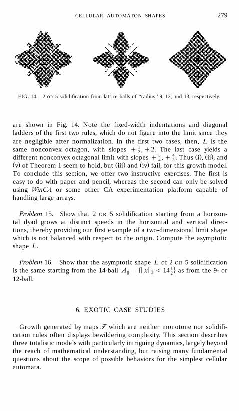
CELLULAR AUTOMATON SHAPES 279
FIG. 14. 2 OR 5 solidification from lattice balls of ‘‘radius’’ 9, 12, and 13, respectively.
are shown in Fig. 14. Note the fixed-width indentations and diagonalladders of the first two rules, which do not figure into the limit since theyare negligible after normalization. In the first two cases, then, L is the
1same nonconvex octagon, with slopes " , "2. The last case yields a23 4 Ž . Ž .different nonconvex octagonal limit with slopes " , " . Thus i , ii , and4 3
Ž . Ž . Ž .v of Theorem 1 seem to hold, but iii and iv fail, for this growth model.To conclude this section, we offer two instructive exercises. The first iseasy to do with paper and pencil, whereas the second can only be solvedusing WinCA or some other CA experimentation platform capable ofhandling large arrays.
Problem 15. Show that 2 OR 5 solidification starting from a horizon-tal dyad grows at distinct speeds in the horizontal and vertical direc-tions, thereby providing our first example of a two-dimensional limit shapewhich is not balanced with respect to the origin. Compute the asymptoticshape L.
Problem 16. Show that the asymptotic shape L of 2 OR 5 solidification1�5 5 4is the same starting from the 14-ball A s x - 14 as from the 9- or20 2
12-ball.
6. EXOTIC CASE STUDIES
Growth generated by maps TT which are neither monotone nor solidifi-cation rules often displays bewildering complexity. This section describesthree totalistic models with particularly intriguing dynamics, largely beyondthe reach of mathematical understanding, but raising many fundamentalquestions about the scope of possible behaviors for the simplest cellularautomata.

GRAVNER AND GRIFFEATH280
Wolfram’s Crystal
Can the asymptotic shape L for a simple CA growth rule be a perfectEuclidean circle? As mentioned at the beginning of this survey, Packard
w xand Wolfram seemed to indicate ‘‘yes’’ in their seminal 1985 paper PW ,both in the passage cited in our Introduction, and later when theysummarize:
w xA remarkable feature of diffusive CA growth is that the boundaries of thepatterns produced do not follow the polytopic form suggested by the underlyinglattice construction of the cellular automaton. Indeed, in many cases, asymptot-ically circular patterns appear to be produced.
The authors cite a few examples of ‘‘diffusive growth,’’ by which theyapparently mean slow linear growth; just how slow is unclear. For instance,they include pictures of the perturbation of Conway’s Life with b s 1�34and s s 1 up to about time 100 starting from a small irregular seed.�2, 3, 44Their final configuration is still quite irregular, but vaguely circular.
The isotropy problem for spatial growth}whether local interacting dy-namics can give rise to an asymptotic shape which is radially symmetric}
w xdates back 40 years to Eden’s Model Ede , in which a new cell isrepeatedly added at a random boundary location of the crystal. For manyyears it was conjectured that L for that model should be isotropic.Although the two- and three-dimensional cases remain open, more recentsupercomputer simulations, and rigorous counterexamples in high dimen-
w xsions Kes2 , provide rather convincing evidence of a residual lattice effectin the limiting geometry of Eden’s Model. We will briefly discuss othershape results for random growth in the next section.
w xFor deterministic CA dynamics, an analysis in GG1 shows that Thresh-old Growth with moderate range r and suitably chosen threshold u canachieve a polygonal asymptotic shape which approximates a circle within2%. We also saw suggestive evidence in the last section that L for the 3 OR
5 rule may be anisotropic with smooth boundary segments. Evidently, then,we are dealing with a very subtle question here which cannot be resolvedby cursory inspection of a few small computer experiments.
w xAbout two years ago we met with Wolfram Wol2 to discuss the isotropyproblem. He confided that, upon closer inspection, the examples men-
w xtioned in PW did not appear to grow with radial symmetry. But hedescribed an exhaustive search of all totalistic CA and mentioned anotherrule which seemed to do the best job of growing circles. Wolfram’s Crystalis another perturbation of Life, with b s 1 and s s 1 . Figure 15�34 �0, 1, 2, 3, 44shows its evolution from a 10-ball after 1000 updates. This preliminarypicture was sufficiently tantalizing that we designed a much larger experi-ment using our CAM-8 ‘‘mixmaster.’’ To test the isotropy conjecture, wecaptured Wolfram’s Crystal every 500 updates until it filled an 8K = 8K

CELLULAR AUTOMATON SHAPES 281
FIG. 15. Wolfram’s Crystal from a 10-ball at time 1000.
array. As a test for circular L, we measured the extent of the growth in theŽhorizontal and 458 directions at times 500, 1000, . . . , 10,000 starting from a
.somewhat larger lattice circle . More precisely, at each such time wecomputed the distance from the origin to the closest hyperplanes touchingthe occupied set, and normal to the 08 and 458 directions. The results ht'and d , together with the eccentricity e [ h r 2 d , are tabulated int t t tTable I. We leave it to the reader to decide whether the numbers supportisotropy, or whether there is a residual eccentricity on the order of a fewper cent. Regardless of the interpretation, a rigorous mathematical solu-tion to either part of our next problem would constitute a major milestonein the theory of cellular automata shapes.
Ž .Problem 17. Find a CA with NN s B for some r, say having anr
asymptotic shape L which is two-dimensional and convex, but not apolygon. Is there such an example for which L is a circle?
Hickerson’s Diamoeba
As nonmonotone cellular automata go, Wolfram’s crystal is quite wellbehaved. Despite its complicated boundary dynamics, the growth spreads

GRAVNER AND GRIFFEATH282
TABLE IHorizontal and Vertical Extent of Wolfram’s Crystal up to Time 10,000
Horizontal DiagonalTime t displacement h displacement d Eccentricity et t t
500 269 180.5 1.0541,000 453 307 1.0431,500 643 432 1.0522,000 823 559.5 1.0402,500 1005 685.5 1.0363,000 1192 810.5 1.0403,500 1368 934.5 1.0354,000 1556 1056 1.0424,500 1746 1183.5 1.0435,000 1931 1310.5 1.0425,500 2110 1436 1.0396,000 2296 1563.5 1.0386,500 2481 1686 1.0417,000 2669 1816.5 1.0397,500 2854 1941.5 1.0398,000 3037 2065.5 1.0408,500 3217 2190.5 1.0389,000 3399 2317.5 1.0379,500 3582 2443 1.037
10,000 3768 2569.5 1.037
steadily}albeit slowly}and appears to acquire a characteristic shape. Byway of contrast, we now introduce an incredibly wild totalistic CA discov-ered by Dean Hickerson, and called the Diamoeba for reasons that willbecome clear shortly. Its birth and survival maps are
b s 1 and s s 1 .�3, 5, 6, 7, 84 �5 , 6, 7, 84
Note that this rule is interfacial. Nevertheless, its evolution from simpleseeds is so complex that we still do not know, or even hazard to guess,whether persistent growth is possible. We extend our gratitude to Hicker-son for letting us describe his findings, some of which have been posted to
Ž .the private LifeList Internet discussion group, but are otherwise unpub-lished.
From small random seeds the Diamoeba typically dies out, although afew configurations have period 2. For instance, the lattice box with fourcells on a side is such a ‘‘blinker.’’ Larger squares with even side length 2ngrow to diamonds of twice the size, but then lock into a period 2 orbit, aswe invite the reader to verify.

CELLULAR AUTOMATON SHAPES 283
Problem 18. Carefully describe the asymptotic behavior of Diamoebafrom lattice boxes with an e¨en number of cells on a side.
Much more interesting is the fate of square seeds B , with odd sidenlength 2n q 1. Early in our experimentation with Hickerson’s Diamoeba,
Ž .we noticed that these initial configurations first grow into near- dia-monds, as in the case of even side length, but then begin a complicatedwithering process until they vanish completely! For instance, Fig. 16 showsthe collapse after B has spread to a 300-diamond, with level sets of the150shrinking boundary drawn using a periodic gray scale palette. We observedthe cyclic occurrence of several distinct polygonal shapes, and suggested toHickerson that the evolution appears recursive. Not only did he confirmour conjecture, but he was also able to obtain an exact expression for thelifetime of the process as a function of n.
During the first n updates the shape is a 12-gon which interpolatesbetween the original square and the maximal diamond. From time n to 2nthe shape is a shrinking 12-gon. After that, most shapes in the collapse are16-gons, some convex, some not, which interpolate between a cycle of 6
FIG. 16. Oscillating collapse from B .150

GRAVNER AND GRIFFEATH284
3 1 3 11 1 2 Žcharacteristic octagons with slopes , , , , , and , respectively along4 2 8 24 2 3.with their negatives, reciprocals, and negative reciprocals . Summation of
an infinite geometric series shows that the time t until death is asymp-ntotic to 12n, while Hickerson’s detailed analysis yields the exact formula
t s 12n y 8 y 4n q 2n q n mod 2 .Ž .n 1 11
Here n and n are the number of 1s and the number of adjacent 11 pairs1 11Žin the binary representation of n. For instance, t s 12 ? 150 y 8 y 4 ? 4150
.q 2 ? 1 q 0 s 1778, as is readily confirmed by experiment. We remarkthat other large, lattice-symmetric seeds such as lattice r-balls are drawntoward this collapsing attractor.
In light of the discussion so far, one might be tempted to conclude thatthe Diamoeba either fixates or dies out, possibly after a modest growthspurt, from any initial seed. However, even moderately large initial config-urations with slight lattice asymmetry can tell a very different story. As anillustration, let us consider seeds of size 2 N y 1: rectangles two cells highand N cells wide, but with the upper right corner cell removed. The casesN F 64 all die by time 10,000, except for N s 34 and 43, which stabilize asperiod 2 blinkers within a few thousand generations, and the four casesN s 54, 59, 61, 63, whose behavior we will now describe in some detail.
The Diamoeba first truly lives up to its name when N s 54 or 59. IfN s 54, then after rapidly forming a rough diamond within the first 25updates, asymmetry at the boundary leads to chaotic time intervals ofgrowth and collapse. Occasional interfacial ‘‘shocks’’ cause size fluctua-tions on the order of the entire crystal. In real time, the growth seemsalmost organic, like the undulations of a single-celled creature. This effectis heightened by the dynamics of virtual cilia which run along Diamoeba’s
Ž .boundary cf. the upper left inset of Fig. 17, for the case N s 59 . The neteffect after 50,000 updates is a blob of more than 50,000 cells, suggesting
Ž .omnivorous growth with a modest appetite . However, at generation52,150 the process seems to stop growing, at least for a very long while. Itsshape is roughly an oblong diamond, a recurring geometry for Diamoeba,while its population fluctuates only a few hundred cells away from 67,500.Examination of the cilia along the edges explains this hiatus. The north-west edge is period 2, except for a small period 8 region at its top. The tophalf of the northeast edge and about the bottom one-third of the southeastedge also have period 2. Three independent boundary regions are stillactive: the lower half of the northeast edge, the upper two-thirds of thesoutheast edge, and the entire southwest edge. Further computation showsthat the northeast region becomes period 4088 in generation 952,824 andthe southeast region becomes period 167,409,998 in generation 731,625,667.Alas, Hickerson has checked that the longest, southwest region remains

CELLULAR AUTOMATON SHAPES 285
FIG. 17. Chaotic growth of Hickerson’s Diamoeba from a 2 = 59 rectangle with one cellremoved.
aperiodic for more than 200 billion updates without experiencing a shockthat destabilizes its shape and starts another growth spurt. The eventualfate of this process remains unresolved. If tempted to conclude that thecrystal has stopped growing, you might ask yourself why. A 3 = 199rectangular seed is instructive in this regard: within about 2500 updates itstabilizes as a ciliated diamond of approximately 13,000 cells, retainsessentially the same formation until shortly after time 99,000, but thenstarts changing shape again.
The case N s 59 is a better candidate for persistent growth, but ends upcreating even more confusion. Figure 17 shows its growth during the first50,000 updates using a cyclic gray scale palette to represent cells added atsuccessive times. The intricate fossil-like striations reflect the chaotic ebband flow of Diamoeba growth. A detail at the upper left shows cilia belowthe right corner. After about 940,000 updates the crystal stops growingtemporarily, with a population of around 41,900,000 cells. Hickerson hasactually identified six different patterns of cilia which arise along the edgesof Diamoeba and can be modeled exactly by one-dimensional CA rules

GRAVNER AND GRIFFEATH286
with boundary conditions. For instance the linear XOR rule arises fre-quently. By isolating the boundary dynamics and feeding them to a 1Dsimulator he is able to predict that one of the cilia regimes will break downafter another 5,191,475 updates, after which another growth spurt ispossible. He speculates that alternating cycles of growth and stasis arise asthe different 1D CA rules compete for supremacy along the boundary, butthat eventually a single rule should attain dominance along each edge ofthe rough diamond, and then, perhaps eons later, the Diamoeba shouldfinally settle into a periodic state.
Growth stops for N s 61 around generation 109,000 with a populationof about a quarter of a million cells. The N s 63 case is settled by time14,276, with an 86 = 86 bounding box and periodic 1D CA dynamics along
Žthe four sides of its diamond. The periods of these rules 1478, 1246, 2936,.and 4628 are small enough that the period of the entire crystal is
computable as 17,572,432,696.For values of N above about 65, there seems to be a kind of nucleation
transition: the great majority of seeds grow to at least a very large size.w xOver the range 65, 85 , only the cases 69 and 73 die out within the first
100,000 updates, none of the others become period 2 within that timeŽ .span, only 77, 80, and 83 appear to have stopped like 54 , and the
remaining 16 cases seem to still be growing, with bounding boxes betweenabout 500 and 1000 cells on a side. Now that our readers are completelybewildered, we finish this subsection with an open problem which canperhaps be resolved by very clever construction of a seed that growsrecursively.
Problem 19. Does Hickerson’s Diamoeba fill Z2 starting from someinitial seed A ?0
Conway’s Life
John Conway’s Game of Life, the totalistic rule with birth and survivalmaps
b s 1 and s s 1�34 �2 , 34
is without question the most celebrated of all cellular automata. Popular-w xized by Martin Gardner in a series of Scientific American articles Gar1
beginning in 1970, the model rapidly became a favorite experimentalplayground of recreational mathematics. For a superb account of the early
w xyears, see volume 2 of BCG . More recently, Conway’s Game has beenrecognized as one of the first and simplest prototypes for the emerging
Ž w x.arena of complex systems theory known as Artificial Life cf. Lan .Perhaps surprisingly, despite the intense scrutiny this rule has received for

CELLULAR AUTOMATON SHAPES 287
nearly 30 years, exciting new discoveries continue to be made, while manyfundamental questions remain unresolved. We are by no means experts,but will attempt to summarize here some recent developments relating topersistent growth from finite seeds. For clarity, the discussion is dividedinto three subsections.
Uni ersality and Pattern Synthesis
One of Life’s most famous properties is computation uni ersality, astronger form of the circuit emulation for Life without Death which wasdescribed in Section 4. The counterparts of LwoD’s ladders are movinggliders, various eaters which can block gliders without being damaged, andglider guns such as the famous 45-cell construct for which Bill Gosper wona $50 prize from Conway. Life does not share LwoD’s propensity forunbridled chaotic growth, so using these ingredients identified in the early1970s, one can simulate a Turing machine with its infinite storage capacity.
w x w xConsult BCG for details, and Min for theoretical background. Refine-Ž w x.ments by Hickerson and Callahan cf. Cal have simplified the construc-
tion and improved its theoretical efficiency.ŽLife experts vouch for the feasibility of a much more powerful and
.complicated extension of the Turing scheme which establishes construc-tion uni ersality, meaning that Life can faithfully simulate any CA rule inspace. Although details of the general construction have never beenspecified, at least in principle Life could then grow from a suitable seed in
Ž w x.the manner of any model described in this paper. D. Bell cf. Calrecently worked out one instance, a unit Life cell which lets Conway’s rulesimulate its own universe. As another illustration of universality, since anycomputer algorithm can be simulated, theoretically it should be possible todesign a Life seed which grows with asymptotic isotropy.
Lest the reader conclude that anything is possible, so there is nothing toknow, we hasten to point out two essential limitations of the simulationapproach. First, it gives no information about how Life evolves startingfrom the preponderance of initial configurations, or from prescribedsimple seeds. Second, even if the goal is to design prescribed dynamics}afinite A with period 17, say, or the delay-line memory architecture of the1949 EDSAC computer}general theory is worthless for a manageableconstruction. Thus, a small group of dedicated researchers continues to doremarkable work on the synthetic understanding of Conway’s rule, assem-bling a huge menagerie of known objects, and interactions between themwhich can be controlled despite Life’s complexity. Paul Callahan’s wonder-
w xful Patterns, Programs, and Links web site Cal features annotated anima-tions of more than a hundred key constructs. Another even more extensive
w xweb site maintained by Mark Niemiec Nie includes contact information

GRAVNER AND GRIFFEATH288
for most of the Life cadre mentioned in this review. Before proceeding toour discussion of persistent growth, let us mention a recent crowningachievement. Based on 10 years of active experimentation by DavidBuckingham with B-heptomino interactions, there is now a general recipefor constructing a finite Life seed of any period greater than 57. Atpresent, only 14 periods are not yet known to arise within elementaryobjects:
19, 23, 27, 31, 33, 34, 37, 38, 39, 41, 43, 49, 51, and 53.
ŽOf these, the values 33, 34, 38, 39, and 51 can be achieved by noninteract-.ing pairs of known objects with the required prime periods.
Breeders and Spacefillers
A glider gun generates persistent growth, albeit in a single direction,since it emits a steady stream of gliders which advance at constant rate.The first example of a Life seed with two-dimensional asymptotic shapewas Gosper’s 4060-cell breeder from the early 1970s. Nowadays the term isused to describe any pattern with a population that grows quadratically bycreating a stream of objects, each of which creates another stream. Figure18 shows the smallest known breeder at present, due to Hickerson. In this
FIG. 18. Hickerson’s 603-cell breeder.

CELLULAR AUTOMATON SHAPES 289
1variant, a ‘‘puffer’’ travels to the right at speed , leaving a steady trail of2
guns behind, each of which emits gliders traveling in the NE direction. Theasymptotic effect is a triangular shape composed completely of gliders,occupying one out of every 45 cells in a regular array:
1 1y1t A ª 1 x dx , where D s 0 - x - x - y x ,Ž . � 4t D 2 1 245 2
Ž .in the sense of 3.3 . A more elaborate and very recent puffer]gliderconstruction by Gosper yields a seed A from which Life evolves so that0every site of Z2 is occupied infinitely often by ‘‘waves of gliders going back
Ž .and forth across a widening river’’ a design proposal of Allan Wechsler ,but such that the occupation times of each x form an aperiodic sequence.
One of the most remarkable Life constructions of the 1990s is Max, thespacefiller. First, the reader should understand that a still life is anyconfiguration which is a fixed point for Conway’s rule. For instance, a
42 = 2 box is a still life. So is the density periodic tiling of the lattice by9
such boxes separated by empty ‘‘frames’’ with width 1. A spacefiller, then,is a seed A such that its limit A exists, and is a still life with positive0 `
density in Z2. The 187-cell seed Max at the upper left of Fig. 19 generates1a density still life by spreading, as shown, in a diamond of alternating2
occupied and vacant horizontal stripes. The delicate ‘‘stretchers’’ at the1corners advance at rate , so2
1 1y1 5 5t A ª 1 x dx , where DD s x F ,Ž . � 41t DD 1r22 21r2
FIG. 19. Stripes generated by Max, a 187-cell Life spacefiller.

GRAVNER AND GRIFFEATH290
Ž .again in the sense of 3.3 . Max has been dieting recently. The designshown here, currently the smallest known spacefiller, incorporates thecombined efforts of H. Holzwart, D. Bell, A. Hensel, and T. Coe. Max isoptimal in two additional respects. First, by comparison with Threshold 3Growth, no Life configuration can advance on an empty background in the
1horizontal or vertical direction at speed greater than . Second, N. Elkies21has shown that is the maximum possible density for a still life. In fact, he2
proves the following beautiful combinatorial generalization:
w x 2THEOREM 4 Elk . If e¨ery site x of configuration A ; Z has at most< < < <three range 1 box neighbors belonging to A, then lim sup A l B r Bnª` n n
1F .2
In the same paper, Elkies obtains analogous sharp upper bounds if‘‘three’’ in his theorem is replaced by any other possible value except‘‘four’’ or ‘‘five,’’ also solves the corresponding range 1 diamond problemcompletely, and discusses generalizations to higher dimensions and othergraphs.
Nucleation Issues
Nothing in our discussion of Conway’s rule so far addresses the issue ofwhether ‘‘typical’’ seeds grow persistently. Most of the smallest configura-tions either die out or rapidly stabilize as a still life or oscillator, perhapsafter emitting a few gliders. Early on, Life experimentalists coined thesomewhat ill-defined notion of a methuselah}a small seed, of less than adozen occupied cells say, which does not stabilize in a recursive pattern fora rather long time, say until at least t s 969. Perhaps the first exampleencountered was the r-pentomino , which stabilizes in generation 1103after producing six gliders.
What, then, is the size of the smallest seed which generates persistentgrowth? This question is still open, although it may not remain so for long.By an exhaustive computer search, Nick Gotts and Paul Callahan havechecked that no initial configuration of 8 or fewer cells grows persistently.Within the past few months Callahan has also discovered a 10-cell seedthat does grow. His method was to test large collections of possibleinteractions between two minimal methuselahs with total population 10.One successful combination arises within a box 35 sites wide and 18 sites
Ž .high: place an r-pentomino oriented as above in the upper left corner,and its 5-cell grandparent in the lower right. After about 2000
iterations the evolution stabilizes, with a steady stream of gliders travelingSW. For now, there remains the possibility of persistent growth from 9initially occupied sites, although Callahan feels he has ruled out ‘‘the mostlikely candidates.’’

CELLULAR AUTOMATON SHAPES 291
As we have seen throughout this paper, even for ‘‘supercritical’’ modelsone only expects persistent growth to be the norm once the initial seed issufficiently large. Thus it is natural to pose
Problem 20. Do most finite Life seeds have infinite population growth?Ž .More precisely, if w n denotes the number of configurations A ; B suchn
< < Ž . < Bn <that A ª `, does w n r2 ª 1 as n ª `?t
Dean Hickerson argues that the answer is undoubtedly ‘‘yes,’’ since a1random huge pattern will include a speed puffer moving outward2
somewhere along its boundary, output from which will cause the totalpopulation to grow. But this assertion is probably quite difficult to provesince some rare structure might conceivably chase along the puffer’s trail,delete its output, and ultimately destabilize the puffer itself, in the mannerof an LwoD shoot overrunning its ladder.
Finally, a most vexing issue is the classification of Conway’s rule as‘‘subcritical, critical, or supercritical.’’ This trichotomy is even hard toformulate for general CA dynamics, but in the spirit of Section 2, super-critical growth should spread over the whole lattice starting from almostany suitably large finite seed, subcritical growth should be unable to fill inlarge holes from typical exterior configurations, and the remaining alterna-tive might well be deemed critical. Since the great preponderance of smallLife seeds either die or stop growing within a few thousand updates, sincethere are apparently no known examples of persistent chaotic growth, and
Žsince Life on a large torus started from random initial conditions e.g., the.default screen saver of SUN Sparcstations for many years eventually
relaxes to a periodic state, it is natural to surmise that Life should besubcritical. On the other hand, attempts have been made to evaluategrowth properties of Life by measuring its ability to propagate finiteperturbations of a disordered equilibrium. Two contradictory conclusions
w xhave emerged: in BCC it was claimed to have a power law tail, and hencew xthat Life enjoys self-organized criticality, whereas BB used larger, more
extensive simulations on a CAM to conclude that effects die off exponen-tially quickly, albeit with a small exponential rate. What seems clear is thatthe Game of Life is remarkably close to critical, by any reasonable
w xdefinition. In this vein, K. Evans Eva has studied higher-range generaliza-tions of Conway’s rule known as Larger than Life, finding a whole parame-terized family of CA rules which are close to critical and support variousgliderlike bugs, breeders, replicators etc. To end on a paranoid note,Problem 19 raises the specter of some exotic, exceedingly rare architecturewith the ability to outcompete any surrounding environment and spreadsupercritically over any environment, in a manner reminiscent of the stable
w xperiodic objects of FGG1 . Life aficionados have never come close toencountering such a creature, but one might be lurking in another galaxy.

GRAVNER AND GRIFFEATH292
7. REMARKS ON RANDOM GROWTH
Chance enters into growth dynamics in two natural ways: either byrandom seeding, i.e., by starting from a random configuration while keepingthe update rule deterministic, or by a random perturbation of the updaterule. In either case, there is a bewildering variety of ways to make therandom assignments, so we will confine our discussion to the simplestchoices. For concreteness, we also restrict the discussion to range 1 boxsolidification rules.
In the case of random seeding, we will assume that the initially occupiedset A is obtained simply by adjoining every site independently with0probability p. Such initializations are convenient since they are relativelyeasy to compute with, and convenient for simulation, while typicallycapturing the essential ergodic behavior of many other translation invari-ant initial states. Since we are dealing with solidification rules, the random
� Ž . 4 Ž Ž . .set A s x: j x s 1 is well defined, and P j 0 s 1 measures the` ` `
final density of occupied sites. The immediate question facing us iswhether the dynamics are likely to fill in most of the lattice under theseconditions. The first of the following two problems is not difficult to solveŽ w x.see GG2 , whereas the second is largely open.
Problem 21. Consider Threshold Growth with threshold u and seedingdensity p. Prove that, for any p ) 0, almost surely, A s Z2 iff u F 4.`
Ž .Also, for the solidification rule which has b i s 1 iff i s 1 or i G 5, showŽ . Ž Ž . . Ž .that for any p g 0, 1 , P j 0 s 1 g 0, 1 .`
Ž Ž . .Problem 22. For Exactly u Growth, when is lim inf P j 0 s 1 )pª 0 `
0? Simulations seem to suggest that this is the case for u F 3. Does the4limit of final densities as p ª 0 exist, and is it equal to for Exactly 19
Growth?
The situation when seeding is sparse, i.e., for p small, is of particularinterest, as it emulates crystal growth caused by rare impurities. In suchcircumstances the rate at which the dynamics fill space is of basic impor-tance, and the natural statistic to measure this rate is T , the first time theorigin is occupied. Simulations make it clear that, in the process of
Ž .covering the lattice, the system evolves through three stages: i nucleationŽ .of occupied areas which are able to grow by themselves, ii growth in a
Ž .slightly polluted environment, and iii interaction between large growingdroplets. Understanding these aspects is crucial for estimating the size ofT. For example, the following theorem holds.
THEOREM 5. Let j be Threshold Growth with threshold u and seedingtdensity p. In supercritical cases, i.e., for u F 3, Tpu con¨erges in distribution

CELLULAR AUTOMATON SHAPES 293
to a nontri ial random ¨ariable as p ª 0. In the critical case u s 4, there existŽ w x.two constants 0 - c - c - ` such that P p ln T g c , c ª 1 as p ª 0.1 2 1 2
Roughly, then, T is of order pyu for supercritical dynamics, and ofexponential size in 1rp for critical dynamics. In the latter case, the originis likely to wait a prolonged time of metastability before it gets occupied.The metastable period, which is exponentially large in a power of 1rp is asignature property of critical thresholds for neighborhoods which are
w x w x w x w xinvariant under 90-degree rotation. References AL , GG2 , GG5 , Mou ,w xand Sch include further discussion of metastability effects in various
models.The more precise statement of Theorem 5 in the supercritical case is
possible because the nucleation positions can be scaled by pu to yield aŽ g .Poisson point location. For general NN , the correct scaling is p . On thisr
scale, the growth and interaction phases involve polygonal shapes whichevolve in a computable way in continuous space and time. We refer the
w xreader to GG2 for a complete proof, but include a problem here whichshould illuminate at least the nucleation ingredient of the argument.
Problem 23. For a general solidification rule, define g as the size of thesmallest initial set A which generates persistent growth. Assuming g - `,0label x g Z2 a nucleus if there exists a set A of g initially occupied sites0
Ž . Ž .such that i A generates persistent growth, and ii x is the leftmost of0yg Ž .the lowest points of A . Compute lim p P x is a nucleus . Then do0 pª 0
Ž . Ž . `Ž . 2the same if i is replaced by i9 T A s Z .0
ŽThe suggested computations more suitable for a computer then a.human should provide some insight about nucleation properties of range
1 solidification rules. For supercritical Threshold Growth, the commonŽvalue of the above two limits determines the intensity number of points
.per unit area of the Poisson point location described above.To illustrate how shape theory applies to related systems, we briefly
mention the Multitype Threshold Voter Model. In this CA one starts witha uniform product measure over k colors on the lattice and, at eachupdate, site x changes to color k iff k is the unique color with at least urepresentatives in x q NN. As k becomes very large, widely separatedregions of single color start expanding, until they eventually induce a
1yu Ždivision of available space. If the space is scaled by k note that u must.be at least 2 for anything to happen , then this division approaches a
Poisson]Voronoi tessellation of R2. This is the object constructed byassigning every point in a Poisson point location PP its own color, and thenpainting every other point in R2 the same color as the closest color in PP.The limit shape L of the corresponding Threshold Growth model deter-
w xmines the norm in which distance is measured. See GG3 .

GRAVNER AND GRIFFEATH294
The rest of this section is devoted to randomly perturbed dynamics.Assuming that growth is generated by a deterministic monotone transfor-
w xmation TT and that p g 0, 1 is a fixed update probability, we confine ourdiscussion to the following simple randomized algorithm:
Ž . 2a Let X , x g Z , t s 0, 1, 2, . . . , be an independent family ofx, tŽ .Bernoulli p random variables, i.e.,
P X s 1 ' p ' 1 y P X s 0 .Ž . Ž .x , t x , t
Ž . Ž .b Start from some deterministic or random set A , independent0of X . Given A , the random set A is determined asx, t t tq1
A j x g TT A : X s 1 .� 4Ž .t t x , t
Such a process is therefore a Markov chain on subsets of Z2. Dynamics inthis vein have been widely studied for more than 20 years. One of the firstand most famous examples, in which TT is Threshold Growth with range 1
w xdiamond neighborhood and u s 1, is called Richardson’s model Ric .ŽRelated threshold 1 systems with random births and random deaths often
. w xrun in continuous time are Eden’s crystal growth Ede , voter modelsw x w xDurr, Toom , and the contact process DG1 . Many papers have beendevoted to shape theory for such local rules. The only known approach issubadditivity, so existence of shapes and rates of convergence are withinreach of rigorous mathematics, but explicit computations are not. Bycontrast, it is possible to explicitly compute shapes when they result fromaggregate behavior of random walks. Two such examples are branchingrandom walks, which are tractable by projection onto lines, in terms ofŽ . w xanisotropic large deviation rates Big ; and Internal DLA, which inherits
wcircular shape from isotropy of the continuum space]time limit LBG,xGQ .
A common feature of the rules described above is that the limitingshape is a convex set, hence about as regular as Euclidean sets can be. At
w xthe opposite extreme are models like DLA WS , which apparently ap-proach some random fractal. Although a lot is known about such dynamics
w xfrom the physics literature BS , rigorous results are few and far between.To reiterate, subadditivity is apparently the only general tool for proving
Ž . Ž .convergence of a random sequence of sets, given by a and b above, toan asymptotic shape. The two alternative approaches described in previoussections}explicit recursion, or identification of half-space velocities}seem hopeless. Moreover, even the subadditivity arguments which havebeen applied to random dynamics rely on a self-evident property ofThreshold 1 Growth: the process can be restarted from any occupied cell.To illustrate how subadditivity works in the presence of randomness, and

CELLULAR AUTOMATON SHAPES 295
how to handle thresholds u ) 1, we will now outline the proof of a shapetheorem for the randomized version of our Basic Example.
THEOREM 6. Consider Random Threshold Growth on the range 1 boxneighborhood, with u s 3 and update probability p ) 0. Then there exists acon¨ex compact neighborhood of the origin, 0 g L ; R2, such that
Hy1 ` 2t A ª L for e¨ery finite A such that TT A s Z .Ž .t 0 0
Proof. Let t denote a geometric random variable with parameter pŽ Ž . Ž .ky1 .i.e., P t s k s p 1 y p ; k G 1 . Moreover, assume that A s0Ž .B 0, 1 ; this entails no loss of generality since a seed which generates the`
plane under TT will cover this square in a finite time under the randomdynamics. Now define
� 4T x s inf t : x g A ,Ž . t
� 4T 9 x s inf t : x q B ; A ,Ž . 1 t
T 9 x , y s inf t : y q B ; A x q B , T 9 x .Ž . Ž .� 4Ž .1 tqT 9Ž x . 1
Ž .Here A B, u is notation for the state of the process at time t q u if ittquX � 4is restarted from B at time u. Write A s x: x q B ; A . Our first stept 1 t
is to prove that A does not extend too far beyond AX .t tŽ . Ž .The lemma from Section 2 implies that T 9 x y T x is bounded above
by the sum of 25 independent copies of t , since in the worst case sitesŽ . Žinside B x, 2 are added one by one. The number 25 can be reduced`
.somewhat. The following crude bound therefore holds for any u G 0:
P T 9 x y T x G u F 25 ? P t G ur25 F 25eyp u r25. 7.1Ž . Ž . Ž . Ž .Ž .tŽ . Ž .2Of course A ; TT A , so A includes at most 2 t q 3 sites. Therefore,t 0 t
for large t,
100P T 9 x y T x ) log t for at least one x g AŽ . Ž . tž /p
3 y4 log tF 2 t q 3 ? 25 ? eŽ .F 200 ? ty2 ,
and hence, by the Borel]Cantelli lemma, there exists a random T such0Ž . Ž . Ž .that T 9 x y T x F 100rp log t for every x g A as soon as t G T . Itt 0
follows that
AX ; A ; AX for t G T . 7.2Ž .t t tqŽ100r p.log t 0
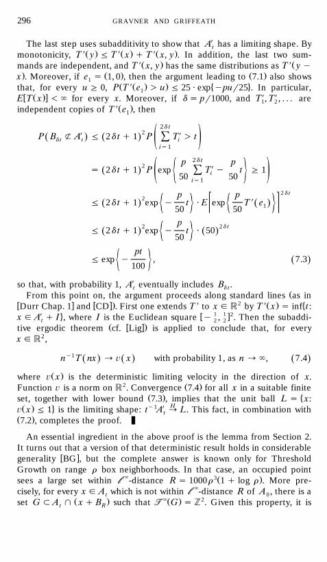
GRAVNER AND GRIFFEATH296
The last step uses subadditivity to show that AX has a limiting shape. BytŽ . Ž . Ž .monotonicity, T 9 y F T 9 x q T 9 x, y . In addition, the last two sum-
Ž . Žmands are independent, and T 9 x, y has the same distributions as T 9 y y. Ž . Ž .x . Moreover, if e s 1, 0 , then the argument leading to 7.1 also shows1
Ž Ž . . � 4that, for every u G 0, P T 9 e ) u F 25 ? exp ypur25 . In particular,1w Ž .x X XE T x - ` for every x. Moreover, if d s pr1000, and T , T , . . . are1 2
Ž .independent copies of T 9 e , then1
2d t2X XP B o A F 2d t q 1 P T ) tŽ . Ž . Ýd t t iž /
is1
2d tp p2 Xs 2d t q 1 P exp T y t G 1Ž . Ý i½ 5ž /50 50is1
2 d tp p2F 2d t q 1 exp y t ? E exp T 9 eŽ . Ž .1½ 5 ½ 550 50p2 2 d tF 2d t q 1 exp y t ? 50Ž . Ž .½ 550
ptF exp y , 7.3Ž .½ 5100
so that, with probability 1, AX eventually includes B .t d tŽFrom this point on, the argument proceeds along standard lines as in
w x w x. 2 Ž . �Durr Chap. 1 and CD . First one extends T 9 to x g R by T 9 x s inf t:X 1 1 24 w xx g A q I , where I is the Euclidean square y , . Then the subaddi-t 2 2
Ž w x.tive ergodic theorem cf. Lig is applied to conclude that, for everyx g R2,
ny1T nx ª ¨ x with probability 1, as n ª `, 7.4Ž . Ž . Ž .
Ž .where ¨ x is the deterministic limiting velocity in the direction of x.2 Ž .Function ¨ is a norm on R . Convergence 7.4 for all x in a suitable finite
Ž . �set, together with lower bound 7.3 , implies that the unit ball L s x:HXy1Ž . 4¨ x F 1 is the limiting shape: t A ª L. This fact, in combination witht
Ž .7.2 , completes the proof.
An essential ingredient in the above proof is the lemma from Section 2.It turns out that a version of that deterministic result holds in considerable
w xgenerality BG , but the complete answer is known only for ThresholdGrowth on range r box neighborhoods. In that case, an occupied point
` 3Ž .sees a large set within ll -distance R s 1000r 1 q log r . More pre-cisely, for every x g A which is not within ll `-distance R of A , there is at 0
Ž . `Ž . 2set G ; A l x q B such that TT G s Z . Given this property, it ist R

CELLULAR AUTOMATON SHAPES 297
not hard to make appropriate modifications in the above proof andconclude that Theorem 6 extends to general box neighborhoods andarbitrary thresholds.
As already mentioned, analytic identification of the limiting shape seemsimpossible for nearly all random growth models. However, partial informa-tion is available in a few instances. The best-known example is Richardson’smodel: if p ) p , the critical probability for oriented site percolation, thenc
w x Žthe shape L has flat edges DLi . It is believed that p f 0.706, but thec.best available rigorous upper bound at present is p - 0.819. It is alsoc
sometimes possible to approximate L in a nearly deterministic model. Forexample, as p ª 1, the shape of Richardson’s model converges to the unitdiamond. A more difficult example is the solidification rule in which a sitewith exactly one of its four nearest neighbors becomes occupied at eachupdate with probability p, while two or more occupied neighbors make itoccupied for sure. In this case, it is not hard to show that the asymptoticshape L exists, but more to the point is that py1r2L converges to ap p
Ž . w xsquare of unknown side as p ª 0 KeSc, Gra2 .Since techniques for explicit computation of limit shapes for random
dynamics are lacking, we resort to Monte Carlo simulation. Running thedynamics from finite sets has some serious drawbacks: the convergence isslow, while strict convexity and differentiability properties are very difficultto detect. A more expeditious approach assumes validity of the polarformula L s KU , and proceeds to estimate the half-space speeds w .p 1r w pp
Efficient estimation of these speeds is possible since one can reducerandom fluctuations by averaging, exploiting the fact that half-spaces aretranslation invariant in one direction. While this approach yields interest-ing results, as we shall see below, it unfortunately has no theoreticalfoundation at present. The models for which half-space velocities can beproved to exist are limited to those which admit either a first-passagew x w xKes2 or last-passage Gra2 representation. Beyond such examples, eventhe special case stated in our next problem remains unresolved at therigorous level. However, this has not stopped physicists from developingvoluminous and sophisticated theory on the regularity of interface motionŽ w x w x.see, e.g., KrSp and BS .
Problem 24. Consider, again, Random Threshold Growth with u s 3.Let A consist of sites on or below the x-axis, and let V ; Z comprise the0 tsecond coordinates of the intersection of A with the y-axis. Show thatt
w e s lim ty1 max V s lim ty1 min Z2 y VŽ . Ž .p 2 t ttª` tª`
exists with probability 1.
Overlooking the current lack of a proof that half-space speeds exist, wenow present some intriguing computer simulations which estimate K1r w p

GRAVNER AND GRIFFEATH298
and L for Random Threshold Growth with u s 3 and various valuesp9 4of p. Figure 20 shows the results for p s 1, , . . . , . Of course the sets K10 10
on the left increase as p decreases, whereas the shapes L on the rightdecrease. These pictures suggest the following behavior for the random-ized version of our Basic Example in various p-regimes:
Ž .a If p is very close to 1, then the convex hull of K is the same aspthe convex hull of K . In this case L s L , so the shape is an explicitly1 p 1computable polygon.
Ž .b As p decreases, eventually the boundary of K no longer inter-psects the boundary of K . In this case the boundary of K is smooth, but if1 pp is not too small, then K is still nonconvex. Hence L has a nondiffer-p p
Ž .entiable boundary i.e., ‘‘corners’’ , but no flat edges.Ž .c Further decreased values of p seem to produce a smooth strictly
convex K . While the mechanism which causes the onset of this regimepremains mysterious, the resulting shapes are apparently smooth and strictlyconvex.
Ž . Ž .Whether or not there is a phase between a and b in which L is not apolygon but still has both corners and flat edges seems too subtle topredict from our simulations, but that fourth scenario seems likely for atleast some choices of neighborhood and threshold. We remark thatsmoothness of the limiting shapes is important in understanding boundary
w xfluctuations of random growth NP . More details on these issues, includ-ing rigorous proofs of some of the observations described above, will
w xappear in a forthcoming research paper BGG .
Ž . Ž .FIG. 20. K left and L right for p s 1, 0.9, . . . , 0.4.1r w pp

CELLULAR AUTOMATON SHAPES 299
One feature of supercritical Threshold Growth models is that smallrandom perturbations do not change their long-term behavior appreciably.
ŽFor instance, in the example just discussed, L ª L as p ª 1 withp 1.equality in a small neighborhood of p s 1 . By contrast, any random
perturbation may destroy the delicate growth pattern of a nonmonotonerule. The reader can either try to work out the solution to our next
Ž w x .problem which is rather difficult; see BN for the appropriate technology ,or else trust Fig. 21, which shows a realization of the Random Exactly 1CA with p s 0.95, after 55 updates, started from a single occupied cell.Note how the fractal pattern of Fig. 6 is completely destroyed.
Problem 25. Consider the Random Exactly 1 CA with update probabil-ity p. Show that, for every e ) 0, there exists a p such that, for every0
Ž .update probability p g p , 1 , a large enough time T exists with probabil-0ity one, so that for any t G T ,
BB ; ty1A q BB1ye t e
Ž .where both boxes above are Euclidean .
In short, the limiting shape, if it exists, is close to the unit square for pclose to 1. The statement in Problem 22 is convoluted since L is notknown to exist. Indeed, except for trivial cases, no techniques are currentlyavailable to prove existence of a limiting shape for any random nonmono-tone model. The relatively simple Random Exactly 1 rule might offer thebest prospects for development of such techniques. We therefore make itthe subject of our last open problem.
FIG. 21. Random Exactly 1 growth from a singleton, p s 0.95.

GRAVNER AND GRIFFEATH300
Problem 26. Show that the Random Exactly 1 rule with update proba-Ž .bility p, started from any nonempty finite seed A , has a unique0
asymptotic shape L.
APPENDIX: CA COMPUTATION ANDVISUALIZATION RESOURCES
w xThe Primordial Soup Kitchen Gri2
http:rrpsoup.math.wisc.edurkitchen.html
is an extensive Web site devoted to cellular automata. Included are anannotated archive of colorful images illustrating the theory and applicationof CA rules, electronic versions of several of our research papers, and the
w xWinCA FG software which was used to perform most of the experimentsdiscussed here, as well as links to other sites on the Internet which dealwith complex spatially distributed systems. A page at the same site
http:rrpsoup.math.wisc.edurjavargrowth.html
has been produced specifically to supplement this article. There the readerwill find a Java applet which runs small-scale, device-independent anima-tions of many of the growth models we have discussed, together withready-made WinCA data files for larger and much faster versions of thesame experiments, and up-to-date Web links to additional resources con-cerning CA shapes.
ACKNOWLEDGMENTS
We are grateful to Tom Bohman, Paul Callahan, Bruce Christenson, Kellie Evans, BobFisch, Cris Moore, Norm Margolus, and Stephen Wolfram for their contributions. Specialthanks to Dean Hickerson for permission to reproduce several of his remarkable experimentsand results.
REFERENCES
w xAL M. Aizenman and J. Lebowitz, Metastability effects in bootstrap percolation, J.Ž .Phys. A 21 1988 , 3801]3813.
w xBan E. R. Banks, Universality in cellular automata, in ‘‘Proc. 11th IEEE SymposiumŽ . Ž .on Foundations of Computer Science FOCS 1970 ,’’ pp. 194]215.
w x Ž .BB C. Bennett and M. Bourzutschky, ‘‘Life’’ not critical?, Nature 350 1991 , 468.w xBCC P. Bak, K. Chen, and M. Creutz, Self-organized criticality in the ‘‘Game of Life,’’
Ž .Nature 342 1989 , 780.

CELLULAR AUTOMATON SHAPES 301
w xBCG E. Berlekamp, J. Conway, and R. Guy, in ‘‘Winning Ways for Your MathematicalPlays,’’ Vol. 2, Chap. 25, Academic Press, New York, 1982.
w xBig J. Biggins, The asymptotic shape of the branching random walk, Ad¨ . in Appl.Ž . Ž .Probab. 10 1 1978 , 62]84.
w xBoh T. Bohman, Discrete Threshold Growth dynamics are omnivorous for box neigh-Ž .borhoods, Trans. Amer. Math. Soc. 1998 , to appear.
w xBG T. Bohman and J. Gravner, Random threshold growth models, 1998, submitted.w xBGG T. Bohman, J. Gravner, and D. Griffeath, Asymptotic shapes for random thresh-
old growth models, 1998, in preparation.w xBH S. Broadbent and J. Hammersley, Percolation processes. I. Crystals and mazes,
Ž .Proc. Cambridge Philos. Soc. 53 1957 , 629]641.w xBN M. Bramson and C. Neuhauser, Survival of one-dimensional cellular automata
Ž .under random perturbations, Ann. Probab. 22 1994 , 244]263.w xBS A.-L. Barabasi and H. Stanley, ‘‘Fractal Concepts in Surface Growth,’’ Cambridge
Univ. Press, Cambridge, UK, 1995.w xCal P. Callahan, Patterns, programs, and links for Conway’s game of Life,
http:rrwww.cs.jhu.edur; callahanrlifepage.html.w xCD J. T. Cox and R. Durrett, Some limit theorems for percolation processes with
Ž .necessary and sufficient conditions, Ann. Probab. 9 1981 , 583]603.w xDura B. Durand, Inversion of 2D cellular automata: Some complexity results, Theoret.
Ž .Comput. Sci. 134 1994 , 387]401.w xDurr R. Durrett, ‘‘Lecture Notes on Particle Systems and Percolation,’’ Wadsworth &
BrooksrCole, Belmont, CA, 1988.w xDG1 R. Durrett and D. Griffeath, Contact processes in several dimensions, Z. Wahrsch.
Ž .¨erw. Gebiete 59 1982 , 535]552.w xDG2 R. Durrett and D. Griffeath, Asymptotic behavior of excitable cellular automata,
Ž .J. Experiment. Math. 2 1993 , 183]208.w xDKS R. Dobrushin, R. Kotecky, and S. Shlosman, ‘‘Wulff Construction, A Global
Shape from Local Interaction,’’ Am. Math. Soc., Providence, 1992.w xDLi R. Durrett and T. Liggett, The shape of the limit set in Richardson’s growth
Ž .model, Ann. Probab. 9 1981 , 186]193.w xDS R. Durrett and J. Steif, Fixation results for the threshold voter models, Ann.
Ž .Probab. 21 1993 , 232]247.w xEE-K G. Ermentrout and L. Edelstein-Keshet, Cellular automata approaches to biolog-
Ž .ical modeling, J. Theoret. Biol. 160 1993 , 97]133.w x Ž .Ede M. Eden, in ‘‘Symp. on Information Theory in Biology’’ H. Yockey, Ed. , p. 359,
Pergamon, New York, 1958.w xElk N. Elkies, The still-Life density problem and its generalizations, preprint, 1997.w xEva K. Evans, ‘‘Larger than Life: It’s So Nonlinear,’’ Ph.D. dissertation, University of
Wisconsin, 1996.w xFG R. Fisch and D. Griffeath, WinCA: A cellular Automaton modeling environment,
Ž w x .Windows 3.xr95 software, version 1.0, 1996. Available from Gri2 .w xFGG1 R. Fisch, J. Gravner, and D. Griffeath, Threshold-range scaling of excitable
Ž .cellular automata, Statist. Comput. 1 1991 , 23]39.w xFGG2 R. Fisch, J. Gravner, and D. Griffeath, Metastability in the Greenberg]Hastings
Ž .model, Ann. Appl. Probab. 3 1993 , 935]967.w xFHP U. Frisch, B. Hasslacher, and Y. Pomeau, Lattice-gas automata for the
Ž .Navier]Stokes equation, Phys. Re¨. Lett. 56 1986 , 1505]1508.w xGar1 M. Gardner, Mathematical games}The fantastic combinations of John Conway’s
Ž . Žnew solitaire game, Life, Scientific American, October 1970 , 120]123. Subse-quent articles about Conway’s Life appeared in the ‘‘Mathematical gamesrcom-

GRAVNER AND GRIFFEATH302
puter recreations’’ column of Scientific American, in the issues of Nov. 1970, Jan.1971, Feb. 1971, Mar. 1971, Apr. 1971, Nov. 1971, Jan. 1972, Dec. 1975, Mar.
.1984, May 1985, Feb. 1987, Aug. 1988, Aug. 1989, Sep. 1989, and Jan. 1990.w xGar2 M. Gardner, ‘‘Wheels, Life and Other Amusements,’’ Freeman, New York, 1983.w xGarz M. Garzon, ‘‘Models of Massive Parallelism: Analysis of Cellular Automata and
Neural Networks,’’ Springer-Verlag, BerlinrNew York, 1995.w xGHH J. Greenberg, B. Hassard, and S. Hastings, Pattern formation and periodic
structures in systems modeled by reaction]diffusion equations, Bull. Amer. Math.Ž .Soc. 84 1978 , 1296]1327.
w xGra1 J. Gravner, The boundary of iterates in Euclidean growth models, Trans. Amer.Ž .Math. Soc. 1996 , 4549]4559.
w xGra2 J. Gravner, Recurrent ring dynamics in two-dimensional cellular automata, 1996,submitted.
w xGG1 J. Gravner and D. Griffeath, Threshold Growth dynamics, Trans. Amer. Math.Ž .Soc. 1993 , 837]870.
w xGG2 J. Gravner and D. Griffeath, First-passage times for discrete Threshold GrowthŽ .dynamics, Ann. Probab. 24 1996 , 1752]1778.
w xGG3 J. Gravner and D. Griffeath, Multitype Threshold Growth: Convergence toŽ .Poisson]Voronoi tessellations, Ann. Appl. Probab. 7 1997 , 615]647.
w xGG4 J. Gravner and D. Griffeath, Nucleation parameters for discrete threshold growthŽ .dynamics, Experiment. Math. 6 1997 , 207]220.
w xGG5 J. Gravner and D. Griffeath, Scaling limits for critical Threshold Growth, 1997, inpreparation.
w xGHR R. Greenlaw, H. Hoover, and W. Ruzzo, ‘‘Limits to Parallel Computation:P-Completeness Theory,’’ Oxford Univ. Press, London, 1995.
w xGN R. Gaylord and K. Nishidate, ‘‘Modeling Nature: Cellular Automata Simulationswith Mathematics,’’ Springer-Verlag, BerlinrNew York, 1996.
w xGQ J. Gravner and J. Quastel, Internal DLA and the Stefan problem, 1998, inpreparation.
w xGri1 D. Griffeath, Self-organization of random cellular automata: Four snapshots, inŽ .‘‘Probability and Phase Transitions’’ G. Grimmett, Ed. , Kluwer Academic,
DordrechtrNorwell, MA, 1994.w xGri2 D. Griffeath, Primordial Soup Kitchen, http:rrpsoup.math.wisc.edurkitchen.
html, World Wide Web.w xGM D. Griffeath and C. Moore, Life without Death is P-complete, 1997, submitted.w xGut H. Gutowitz, Frequently asked questions about cellular automata,
http:rralife.santafe.eduralifertopicsrcasrca-faqrca-faq.html, World Wide Web.w xHar J. Hartmanis, On the computing paradigm and computational complexity, in
Ž .‘‘MFCS’95’’ J. Wiederman and P. Hajek, Eds. , Lecture Notes in ComputerScience, Vol. 969, pp. 82]92, Springer-Verlag, BerlinrNew York, 1995.
w xHol J. Holland, Outline for a logical theory of adaptive systems, and other articles, inŽ .‘‘Essays on Cellular Automata’’ A. W. Burks, Ed. , Univ. of Illinois Press,
Champaign, 1970.w xJen E. Jen, Exact solvability and quasiperiodicity of one-dimensional cellular au-
Ž .tomata, Nonlinearity 4 1991 , 251]276.w xJM W. Johnson and R. Mehl, Reaction kinetics in processes of nucleation and
Ž .growth, Trans. A. I.M.M.E. 135 1939 , 416]458.w xKar J. Kari, Reversability of 2D cellular automata is undecidable, Physica D 45
Ž .1990 , 379]385.

CELLULAR AUTOMATON SHAPES 303
w xKes1 H. Kesten, First passage percolation and a higher-dimensional generalization, inŽ .‘‘Particle Systems, Random Media and Large Deviations’’ R. Durrett, Ed. , Am.
Math. Soc., Providence, 1984.w xKes2 H. Kesten, On the speed of convergence in first-passage percolation, Ann. Appl.
Ž .Probab. 4 1994 , 76]107.w xKeSc H. Kesten and R. Schonmann, On some growth models with a small parameter,
Ž .Probab. Theory Related Fields 101 1995 , 435]468.w xKrSp J. Krug and H. Spohn, Kinetic roughening of growing surfaces, in ‘‘Solids far from
Ž .Equilibrium,’’ C. Godreche, Ed. , pp. 479]582, Cambridge Univ. Press, Cam-bridge, UK, 1992.
w x Ž .Lan C. Langton, Studying artificial life with cellular automata, Physica D 22 1986 ,120]149.
w xLBG G. Lawler, M. Bramson, and D. Griffeath, Internal diffusion limited aggregation,Ž .Ann. Probab. 14 1992 , 2117]2140.
w xLDKB A. Lawniczak, D. Dab, R. Kapral, and J.-P. Boon, Reactive lattice gas automata,Ž .Physica D 47 1991 , 132]158.
w xLig T. Liggett, ‘‘Interacting Particle Systems,’’ Springer-Verlag, BerlinrNew York,1985.
w xLin D. Lind, Applications of ergodic theory and sofic systems to cellular automata,Ž .Physica D 10 1984 , 36]44.
w xLN K. Lindgren and M. Nordahl, Universal computation in simple one-dimensionalŽ .cellular automata, Complex Systems 4 1990 , 299]318.
w xMarg N. Margolus, ‘‘CAM-8: A Virtual Processor Cellular Automata Machine,’’ MITLaboratory for Computer Science, 1995.
w xMart B. Martin, A universal cellular automaton in quasi-linear time and its S-m-nŽ .form, Theoret. Comput. Sci. 123 1994 , 199]237.
w xMin M. Minsky, ‘‘Computation: Finite and Infinite Machines,’’ Prentice Hall, NewYork, 1972.
w xMou T. Mountford, Critical lengths for semi-oriented bootstrap percolation, StochasticŽ .Process. Appl. 95 1995 , 185]205.
w xNie M. Niemiec, Life Page, http:rrhome.sprynet.comr interservr mniemiecrlifepage.htm.
w xNP C. Newman and M. Piza, Divergence of shape fluctuations in two dimensions,Ž .Ann Probab. 23 1995 , 977]1005.
w x Ž .NM M. Nowak and R. May, Evolutionary games and spatial chaos, Nature 359 1992 ,826]829.
w xPac N. Packard, ‘‘Cellular Automaton Models for Dendritic Crystal Growth,’’ Insti-tute for Advanced Study, 1985.
w xPap C. Papadimitriou, ‘‘Computational Complexity,’’ Addison-Wesley, Reading, MA,1994.
w xPW N. Packard and S. Wolfram, Two-dimensional cellular automata, J. Statist. Phys.Ž .38 1985 , 901]946.
w xRic D. Richardson, Random growth in a tesselation, Proc. Cambridge Philos. Soc. 74Ž .1973 , 515]528.
w x Ž .San L. Sander, Fractal growth processes, Nature 322 1986 , 789]793.w xSch R. Schonmann, On the behavior of some cellular automata related to bootstrap
Ž .percolation, Ann. Probab. 20 1992 , 174]193.w xTCH J. Taylor, J. Cahn, and C. Handwerker, Geometric models of crystal growth
Ž . Ž .Overview No. 98-1 , Acta Met. 40 1992 , 1443]1474.w xTM T. Toffoli and N. Margolus, ‘‘Cellular Automata Machines}A New Environment
for Modeling,’’ MIT Press, Cambridge, MA, 1987.

GRAVNER AND GRIFFEATH304
w xToom A. Toom, Cellular automata with errors: Problems for students of probability, inŽ .‘‘Topics in Contemporary Probability and Its Applications’’ J. L. Snell, Ed. , CRC
Press, Boca Raton, FL, 1995.w x Ž .Ula S. Ulam, Random processes and transformations, in ‘‘Proc. 1950 Int. Congr.
Ž .Math.,’’ Vol. 2, pp. 264]275 1952 .w x Ž .Vic G. Vichniac, Simulating physics with cellular automata, Physica D 10 1984 ,
96]115.w xvK H. von Koch, 1904.w x Ž .vN J. von Neumann, ‘‘Theory of Self-Reproducing Automata’’ A. Burks, Ed. , Univ.
of Illinois Press, Champaign, 1966.w xWR N. Weiner and A. Rosenblueth, The mathematical formulation of the problem of
conduction of impulses in a network of connected excitable elements, specificallyŽ .in cardiac muscle, Arch. Inst. Cardiol. Mexico 16 1946 , 205]265.
w xWS T. Witten and L. Sander, Diffusion limited aggregation, Phys. Re¨ . Lett. 47Ž .1981 , 1400]1403.
w x Ž . Ž .Wil1 S. Willson, On convergence of configurations, Discrete Math. 23 3 1978 ,279]300.
w x Ž .Wil2 S. Willson, Cellular automata can generate fractals, Discrete Appl. Math. 8 1Ž .1984 , 91]99.
w xWol1 S. Wolfram, ‘‘Cellular Automata and Complexity,’’ Addison-Wesley, Menlo Park,CA, 1994.
w xWol2 S. Wolfram, private communication, 1995.


![Janko Gravner gravner@math.ucdavis.edu Genna Gliner …gravner/replication/rep.pdf · 2011. 2. 17. · Rule 126 [Jen2, Jen3, GG3]. It has binary states and its rule mandates that](https://static.fdocuments.net/doc/165x107/6100d7b11c1b361c004db305/janko-gravner-gravnermath-genna-gliner-gravnerreplicationreppdf-2011-2.jpg)